Understanding Deep Representation Learning via Layerwise Feature Compression and Discrimination

Abstract

Over the past decade, deep learning has proven to be a highly effective tool for learning meaningful features from raw data. However, it remains an open question how deep networks perform hierarchical feature learning across layers. In this work, we attempt to unveil this mystery by investigating the structures of intermediate features. Motivated by our empirical findings that linear layers mimic the roles of deep layers in nonlinear networks for feature learning, we explore how deep linear networks transform input data into output by investigating the output (i.e., features) of each layer after training in the context of multi-class classification problems. Toward this goal, we first define metrics to measure within-class compression and between-class discrimination of intermediate features, respectively. Through theoretical analysis of these two metrics, we show that the evolution of features follows a simple and quantitative pattern from shallow to deep layers when the input data is nearly orthogonal and the network weights are minimum-norm, balanced, and approximate low-rank: Each layer of the linear network progressively compresses within-class features at a geometric rate and discriminates between-class features at a linear rate with respect to the number of layers that data have passed through. To the best of our knowledge, this is the first quantitative characterization of feature evolution in hierarchical representations of deep linear networks. Empirically, our extensive experiments not only validate our theoretical results numerically but also reveal a similar pattern in deep nonlinear networks which aligns well with recent empirical studies. Moreover, we demonstrate the practical implications of our results in transfer learning. Our code is available at https://github.com/Heimine/PNC_DLN.

Key words: deep representation learning, neural networks, intermediate features, feature compression and discrimination

1 Introduction

1.1 Background and Motivation

In the past decade, deep learning has exhibited remarkable success across a wide range of applications in engineering and science [70], such as computer vision [56, 103], natural language processing [102, 109], and health care [36], to name a few. It is commonly believed that one major factor contributing to the success of deep learning is its ability to perform hierarchical feature learning: Deep networks can leverage their hierarchical architectures to extract meaningful and informative features from raw data [10, 65]. Despite recent efforts to understand deep networks, the underlying mechanism of how deep networks perform hierarchical feature learning across layers still remains a mystery, even for classical supervised learning problems, such as multi-class classification. Gaining a deeper insight into this question will offer theoretical principles to guide the design of network architectures [51], shed light on generalization and transferability [75], and facilitate network training [112].

Empirical results on feature expansion and compression.

Towards opening the black box of deep networks, extensive empirical research has been conducted by investigating outputs at each layer of deep networks in recent years. An intriguing line of research has empirically investigated the role of different layers in feature learning; see, e.g., [1, 7, 25, 34, 79, 91, 119]. In general, these empirical studies demonstrate that the initial layers expand the intrinsic dimension of features to make them linearly separable, while the subsequent layers compress the features progressively; see Figure 1. For example, in image classification tasks, [1] observed that the features of intermediate layers are more and more linearly separable as we reach the deeper layers. Recent works [7, 91] studied the evolution of the intrinsic dimension of intermediate features across layers in trained networks using different metrics. They both demonstrated that the dimension of the intermediate features first blows up and later goes down from shallow to deep layers. More recently, [79] delved deeper into the role of different layers, and concluded that the initial layers create linearly separable intermediate features, and the subsequent layers compress these features progressively.

(a) A 7-layer MLP network with ReLU

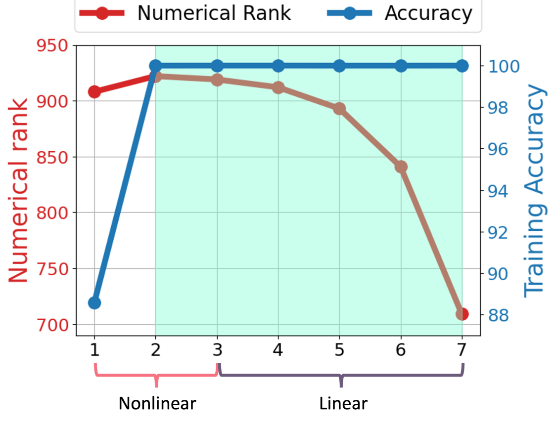
(b) A 7-layer hybrid network

Figure 1: Illustration of numerical rank and training accuracy across layers. We train two networks with different architectures on the CIFAR-10 dataset: (a) A 7-layer multilayer perceptron (MLP) network with ReLU activation, (b) A hybrid network formed by 3-layer MLP with ReLU activation followed by a 4-layer linear network. For each figure, we plot the numerical rank of the features of each layer and training accuracy by applying linear probing to the output of each layer against the number of layers, respectively. The green shade indicates that the features at these layers are approximately linearly separable, as evidenced by the near-perfect accuracy achieved by a linear classifier. The definition of numerical rank and more experimental setups are deferred to Section 5.1.1.

Empirical results on feature compression and discrimination.

In the meanwhile, recent works [87, 50, 37, 120] provided more systematic studies into structures of intermediate features. They revealed a fascinating phenomenon during the terminal phase of training deep networks termed neural collapse (NC), across many different datasets and model architectures. Specifically, NC refers to a training phenomenon in which the last-layer features from the same class become nearly identical, while those from different classes become maximally linearly separable. In other words, deep networks learn within-class compressed and between-class discriminative features. Building upon these studies, a more recent line of work investigated the NC properties at each layer to understand how features are transformed from shallow to deep layers; see, e.g., [17, 51, 47, 42, 92]. In particular, [51] empirically showed that a progressive NC phenomenon governed by a law of data separation occurs from show to deep layers. The works [17, 42] provided empirical evidence confirming the occurrence of an NC property called nearest class-center separability in intermediate layers. [92] empirically showed that similar NC properties appear in intermediate layers during training, where the within-class variance decreases relative to the between-class variance as layers go deeper.

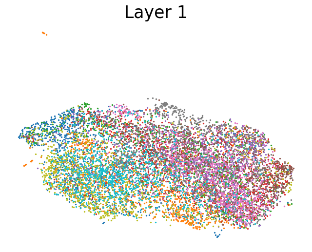
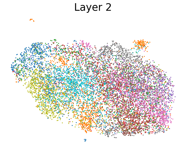
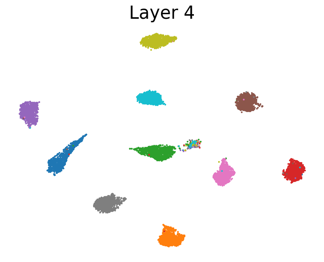
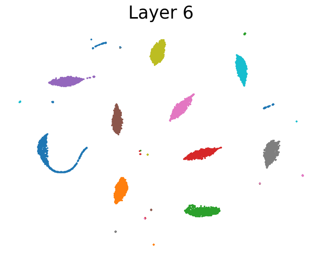
(a) A 7-layer nonlinear MLP

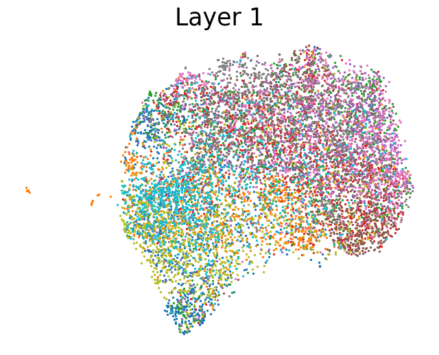
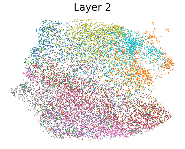
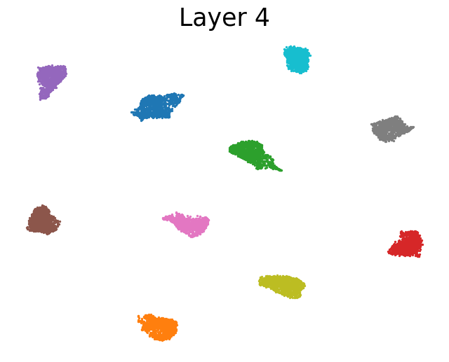
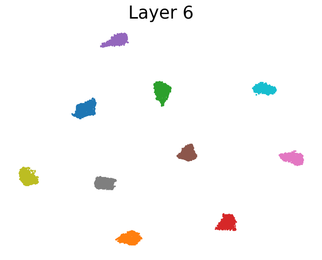
(b) A hybrid network with 3-layer MLP + 4-layer DLN

Figure 2: Visualization of feature compression & discrimination from shallow to deep layers. We consider the same setup as in Figure 1. For each network, we visualize the outputs of layers 1, 2, 4, and 6 on the CIFAR10 dataset using the 2-dimensional UMAP plot [77]. More experimental setups are deferred to Section 5.1.1.

In summary, extensive empirical results demonstrate that after feature expansion by initial layers, deep networks progressively compress features within the same class and discriminate features from different classes from shallow to deep layers; see also Figure 2. This characterization provides valuable insight into how deep networks transform data into output across layers in classification problems. Moreover, this insight sheds light on designing more advanced network architectures, developing more efficient training strategies, and achieving better interpretability. However, to the best of our knowledge, no theory has been established to explain this empirical observation of progressive feature compression and discrimination. In this work, we make the first attempt to provide a theoretical analysis of this observation based on deep linear networks (DLNs) to bridge the gap between the practice and theory of deep representation learning.

Why study DLNs? Linear layers mimic deep layers in nonlinear networks for feature learning.

Even though DLNs lack the complete expressive power of nonlinear networks, they possess comparable abilities for feature compression and discrimination to those found in the deeper layers of nonlinear networks, as indicated in Figures 1 and 2. By assessing the training accuracy and the numerical rank of intermediate features in both a nonlinear network and a hybrid network, it becomes apparent that the initial-layer features in both networks are almost linearly separable, evidenced by nearly perfect training accuracy achieved through linear probing. This phenomenon is further exemplified by the feature visualization presented in Figure 2. In the meanwhile, the linear layers in the hybrid network replicate the role of the counterpart in the nonlinear network to do feature compression and discrimination, as evidenced by the declining feature rank in Figure 1 and the increasing separation of different-class features in Figure 2 across layers in both types of networks.

Broadly speaking, DLNs have been recognized as valuable prototypes for investigating nonlinear networks due to the resemblance of certain behaviors in their nonlinear counterparts [1, 7, 79, 91] and their simplicity [3, 41, 95, 96]. For instance, [49] empirically demonstrated the presence of a low-rank bias at both initialization and after training for both linear and nonlinear networks. [96] showed that a DLN exhibits a striking hierarchical progressive differentiation of structures in its internal hidden representations, resembling patterns observed in their nonlinear counterparts.

The role of depth in DLNs: improving generalization, feature compression, and training speed.

Although stacking linear layers in DLNs ultimately results in an end-to-end linear transformation from the input to the output, the overparameterization present in these DLNs sets them apart from a basic linear operator: increasing the depth of DLNs can significantly improve their generalization capabilities, enhance feature compression, and facilitate network training. Specifically, recent works demonstrated that linear over-parameterization by depth (i.e., expanding one linear layer into a composition of multiple linear layers) in deep nonlinear networks yields better generalization performance across different network architectures and datasets [39, 49, 68]. This is also corroborated by our experiments in Figure 3, where increasing the depth of linear layers of a hybrid network leads to improved test accuracy. Moreover, our results in Figure 12 imply that increasing depth of DLN also leads to improved feature compression. On the other hand, Arora et al. [3] showed that linear over-parameterization, such as increasing depth, acts as a preconditioner, which can accelerate convergence in DLNs. We refer interested readers to [84] for further discussion on the role of depth in DLNs.

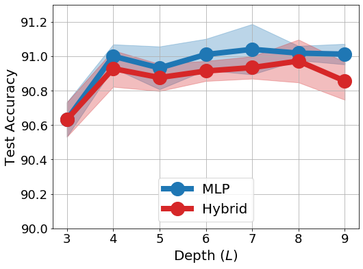
(a) FashionMNIST

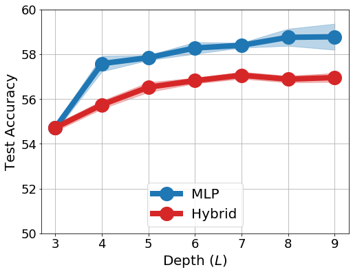
(b) CIFAR-10

Figure 3: Depth of DLNs lead to better generalization performance. We train hybrid networks consisting of a 2-layer MLP with ReLU activation followed by $(L-2)$ linear layers on the FashionMNIST and CIFAR-10 datasets, respectively. As a reference, we also train nonlinear networks comprised exclusively of MLP layers. We plot the test accuracy against the different number of layers averaged over $5$ different runs. It is observed that adding linear layers and MLP layers can both yield better generalization performance. More experimental setups are deferred to Section 5.1.2.

1.2 Our Contributions

In this work, we study hierarchical representations of deep networks for multi-class classification problems. Toward this goal, we explore how a DLN transforms input data into a one-hot encoding label matrix from shallow to deep layers by investigating features at each layer. To characterize the structures of intermediate features, we define metrics to measure within-class feature compression and between-class feature discrimination at each layer, respectively. We establish a unified framework to analyze these metrics and reveal a simple and quantitative pattern in the evolution of features from shallow to deep layers:

More specifically, we rigorously prove the above claim based upon the assumption that

• Assumption on the training data. We study a $K$-class classification problem with balanced training data, where the number of training samples in each class is $n$. We assume that the training input samples are $\theta$-nearly orthonormal for a constant $\theta\in[0,1/4)$, and the feature dimension is larger than the total number of samples so that they are linearly separable.

• Assumption on the trained weights. We assume that an $L$-layer DLN is trained such that its weights are minimum-norm, $\delta$-balanced, and $\varepsilon$-approximate low-rank due to the implicit bias of gradient descent, where $\delta,\varepsilon\in(0,1)$ is a constant.

We discuss the validity of our assumptions in Section 3.2. Based upon the above, we show in Section 3.1 that the ratio of within-class feature compression metric between the $(l+1)$-th layer and the $l$-th layer is determined by $O(\varepsilon^{2}/n^{1/L})$, implying a layerwise geometric decay from shallow to deep layers. On the other hand, we show that the metric of between-class discrimination increases linearly with respect to (w.r.t.) the number of layers, with a slope of $O((\theta+4\delta)/L)$. To the best of our knowledge, this is the first quantitative characterization of the feature evolution in hierarchical representations of DLNs in terms of feature compression and discrimination. In particular, this analysis framework can be extended to nonlinear networks. Finally, we substantiate our theoretical findings in Section 5 for both synthetic and real-world datasets, demonstrating that our claims are true for DLNs and also manifest in nonlinear networks empirically.

Significance of our results.

In recent years, there has been a growing body of literature studying hierarchical feature learning to open the black box of deep networks. These studies include recent works on neural tangent kernel [58, 54], intermediate feature analysis [1, 79, 92], neural collapse [32, 51, 97, 105], and learning dynamic analysis [10, 12, 31], among others; we refer readers to Section 4 for a more comprehensive discussion. Our work contributes to this emerging area by showing that each layer of deep networks plays an equally important role in hierarchical feature learning, which compresses within-class features at a geometric rate and discriminates between-class features at a linear rate w.r.t. the number of layers. This provides a simple and precise characterization of how deep networks transform data hierarchically from shallow to deep layers. It also addresses an open question about neural collapse, and offers a new perspective justifying the importance of depth in feature learning. Moreover, our result explains why projection heads [21], which usually refer to one or several MLP layers added between the feature layer and final classifier during pretraining and discarded afterwards, can improve the performance of transfer learning on downstream tasks [75, 63, 43]. To sum up, our result provides important guiding principles for deep learning practices related to interpretation, architecture design, and transfer learning.

Differences and connections to the existing literature.

Finally, we would like to highlight the differences and connections between our work and two closely related recent results [51, 96] in the following.

• First, [51] empirically showed that a progressive NC phenomenon governed by a law of data separation occurs from shallow to deep layers. Specifically, they observed that in trained over-parameterized nonlinear networks for classification problems, a metric of data separation decays at a geometric rate w.r.t. the number of layers. This is similar to our studied within-class feature compression at a geometric rate, albeit with different metrics (see the remark after 1). However, they do not provide any theoretical explanation for the progressive NC phenomenon. While our research focuses on DLNs and may not provide a complete understanding of phenomena in nonlinear networks, our theoretical analysis of DLNs can offer insights into what we observe empirically in the deeper, nonlinear layers of such networks. This is supported by our findings presented in Figure 1, which show that linear layers can replicate the function of deep nonlinear layers in terms of feature learning.

• Second, [96] reveals that during training, nonlinear neural networks exhibit a hierarchical progressive differentiation of structure in their internal representations—a phenomenon they refer to as progressive differentiation. While both their and our studies revealed and justified a progressive separation phenomenon based on DLNs, the focuses are entirely different yet highly complimentary to each other. Specifically, we investigate how a trained neural network separates data according to their class membership from shallow to deep layers after training, while they investigate how weights of a neural network change w.r.t. training time and their impact on class differentiation during training. This can be illustrated through the example in [96]. Suppose we train a neural network to classify eight items: sunfish, salmon, canary, robin, daisy, rose, oak, and pine. We study how these eight items are represented by the neural networks from shallow to deep layers in a trained neural network. In comparison, [96] explain why animals versus plants are first distinguished at the initial stage of training, then birds versus fish, then trees versus flowers, and then finally individual items in the whole training process.

1.3 Notation & Paper Organization

Notation.

Let $\mathbb{R}^{n}$ be the $n$-dimensional Euclidean space and $\|\cdot\|$ be the Euclidean norm. For a given matrix $\bm{A}\in\mathbb{R}^{m\times n}$, we use $\bm{a}_{i}$ to denote its $i$-th column; we use $\|\bm{A}\|_{F}$ to denote the Frobenius norm of $\bm{A}$; we use $\sigma_{\max}(\bm{A})$ (or $\|\bm{A}\|$), $\sigma_{i}(\bm{A})$, and $\sigma_{\min}(\bm{A})$ to denote the largest, the $i$-th largest, and the smallest singular values, respectively. We use $\bm{A}^{\dagger}$ to denote the pseudo-inverse of a matrix $\bm{A}$. Given $L\in\mathbb{N}$, we use $[L]$ to denote the index set $\{1,\cdots,L\}$. Let $\mathcal{O}^{n}=\{\bm{Z}\in\mathbb{R}^{n\times n}:\bm{Z}^{T}\bm{Z}=\bm{I}\}$ denote the set of $n\times n$ orthogonal matrices. We denote the Kronecker product by $\otimes$. Given weight matrices $\bm{W}_{1},\dots,\bm{W}_{L}$, let $\bm{W}_{l:1}:=\bm{W}_{l}\dots\bm{W}_{1}$ be a matrix multiplication from $\bm{W}_{l}$ to $\bm{W}_{1}$ for all $l\in[L]$.

Organization.

The rest of the paper is organized as follows. In Section 2, we introduce the basic settings of our problem. In Section 3, we describe the main result of our work and discuss its implications, with proofs provided in Section B in the appendix. In Section 4, we discuss the relationship of our results to related works. In Section 5, we verify our theoretical claims and investigate nonlinear networks via numerical experiments. Finally, we draw a conclusion and discuss future directions in Section 6. We defer all the auxiliary technical results to the appendix.

2 Preliminaries

In this section, we first formally set up the problem of training DLNs for solving multi-class classification problems in Section 2.1, followed by introducing the metrics for measuring within-class compression and between-class discrimination of features at each layer in Section 2.2.

2.1 Problem Setup

Multi-class classification problem.

We consider a $K$-class classification problem with training samples and labels $\{(\bm{x}_{k,i},\bm{y}_{k})\}_{i\in[n_{k}],k\in[K]}$, where $\bm{x}_{k,i}\in\mathbb{R}^{d}$ is the $i$-th sample in the $k$-th class, and $\bm{y}_{k}\in\mathbb{R}^{K}$ is an one-hot label vector with the $k$-th entry being $1$ and $0$ elsewhere. We denote by $n_{k}$ the number of samples in the $k$-th class for each $k\in[K]$. Here, we assume that the number of samples in each class is the same, i.e., $n_{1}=\cdots=n_{K}=n$. Moreover, we denote the total number of samples by $N=nK$. Without loss of generality, we can arrange the training samples in a class-by-class manner such that

$$\bm{X}\;=\;\left[\bm{x}_{1,1},\ldots,\bm{x}_{1,n_{1}},\ldots,\bm{x}_{K,1},\ldots,\bm{x}_{K,n_{K}}\right]\in\mathbb{R}^{d\times N},\quad\bm{Y}\;=\;\bm{I}_{K}\otimes\bm{1}_{n}^{T}\in\mathbb{R}^{K\times N},$$ (1)

where $\otimes$ denotes the Kronecker product. Note that we also use $\bm{x}_{i}$ to denote the $i$-th column of $\bm{X}$.

DLNs for classification problems.

In this work, we consider an $L$-layer ($L\geq 2$) linear network $f_{\bm{\Theta}}(\cdot):\mathbb{R}^{d}\rightarrow\mathbb{R}^{K}$, parameterized by $\bm{\Theta}=\{\bm{W}_{l}\}_{l=1}^{L}$ with input $\bm{x}\in\mathbb{R}^{d}$, i.e.,

$$f_{\bm{\Theta}}(\bm{x})\;:=\;\bm{W}_{L}\cdots\bm{W}_{1}\bm{x}\;=\;\bm{W}_{L:1}\bm{x},$$ (2)

where $\bm{W}_{1}\in\mathbb{R}^{d_{1}\times d}$, $\bm{W}_{l}\in\mathbb{R}^{d_{l}\times d_{l-1}}\;(l=2,\dots,L-1)$, and $\bm{W}_{L}\in\mathbb{R}^{K\times d_{L-1}}$ are weight matrices. It is worth mentioning that the last-layer weight $\bm{W}_{L}$ is referred to as the linear classifier and the output of the $l$-th layer as the $l$-th layer feature for all $l\in[L-1]$ in the literature. As discussed in Section 1, DLNs are often used as prototypes for studying practical deep networks [48, 62, 69, 73, 95]. Then, we train an $L$-layer linear network to learn weights $\bm{\Theta}=\{\bm{W}_{l}\}_{l=1}^{L}$ via minimizing the mean squared error (MSE) loss between $f_{\bm{\Theta}}(\bm{x})$ and $\bm{y}$, i.e.,

$$\min_{\bm{\Theta}}\ell(\bm{\Theta})\;=\;\frac{1}{2}\sum_{k=1}^{K}\sum_{i=1}^{n_{k}}\left\|\bm{W}_{L:1}\bm{x}_{k,i}-\bm{y}_{k}\right\|^{2}\;=\;\frac{1}{2}\|\bm{W}_{L:1}\bm{X}-\bm{Y}\|_{F}^{2}.$$ (3)

Before we proceed, we make some remarks on this problem.

• First, the cross-entropy (CE) loss is arguably the most popular loss function used to train neural networks for classification problems [120]. However, recent studies [46, 121] have demonstrated through extensive experiments that the MSE loss achieves comparable or even superior performance than the CE loss across various tasks.

• Second, while DLNs may appear simple, their loss landscapes, as defined in (3), are highly nonconvex, leading to highly nonlinear learning dynamics in gradient descent (GD). Notably, the nonlinear GD dynamics in DLNs closely mirror that in their nonlinear counterparts [71, 95, 96].

• Finally, DLNs tend to be over-parameterized, with width of networks $d_{l}$ and feature dimensions $d$ exceeding the training samples $N$. In this context, Problem (3) has infinitely many solutions that can achieve zero training loss, i.e., $\bm{W}_{L:1}\bm{X}=\bm{Y}$. However, many studies have delved into the convergence behavior of GD by closely examining its learning trajectory. These investigations reveal that GD, when initialized appropriately, exhibits an implicit bias towards minimum norm solutions [14, 82] with approximately balanced and low-rank weights [2, 82], which will be discussed further Section 3.2.

2.2 The Metrics of Feature Compression and Discrimination

In this work, we focus on studying feature structures at each layer in a trained DLN. Given the weights $\bm{\Theta}=\{\bm{W}_{l}\}_{l=1}^{L}$ satisfying $\bm{W}_{L:1}\bm{X}=\bm{Y}$, by construction the weights $\{\bm{W}_{l}\}_{l=1}^{L}$ of the DLN transform the input data $\bm{X}$ into the membership matrix $\bm{Y}$ at the final layer. However, the hierarchical structure of the DLN prevents us from gaining insight into the underlying mechanism of how it transforms the input data into output from shallow to deep layers. To unravel this puzzle, we probe the features learned at intermediate layers. In our setting, we write the $l$-th layer’s feature of an input sample $\bm{x}_{k,i}$ as

$$\bm{z}_{k,i}^{l}=\bm{W}_{l}\dots\bm{W}_{1}\bm{x}_{k,i}=\bm{W}_{l:1}\bm{x}_{k,i},\ \forall l=1,\dots,L-1,$$ (4)

and we denote $\bm{z}_{k,i}^{0}=\bm{x}_{k,i}$. For $l=0,1,\dots,L-1$, let $\bm{\Sigma}_{W}^{l}$ and $\bm{\Sigma}_{B}^{l}$ respectively denote the sum of the within-class and between-class covariance matrices for the $l$-th layer, i.e.,

$$\bm{\Sigma}_{W}^{l}:=\frac{1}{N}\sum_{k=1}^{K}\sum_{i=1}^{n_{k}}\left(\bm{z}_{k,i}^{l}-\bm{\mu}_{k}^{l}\right)\left(\bm{z}_{k,i}^{l}-\bm{\mu}_{k}^{l}\right)^{T},$$ (5)

$$\bm{\Sigma}_{B}^{l}:=\frac{1}{N}\sum_{k=1}^{K}n_{k}\left(\bm{\mu}_{k}^{l}-\bm{\mu}^{l}\right)\left(\bm{\mu}_{k}^{l}-\bm{\mu}^{l}\right)^{T},$$ (6)

where

$$\bm{\mu}_{k}^{l}=\frac{1}{n_{k}}\sum_{i=1}^{n_{k}}\bm{z}_{k,i}^{l},\quad\bm{\mu}^{l}=\frac{1}{K}\sum_{k=1}^{K}\bm{\mu}_{k}^{l}$$ (7)

denote the mean of the $l$-th layer’s features in the $k$-th class and the global mean of the $l$-th layer’s features, respectively. Equipped with the above setup, we can measure the compression of features within the same class and the discrimination of features between different classes using the following metrics.

Definition 1.

For all $l=0,1,\dots,L-1$, we say that

$$\boxed{\quad C_{l}=\frac{\mathrm{Tr}(\bm{\Sigma}_{W}^{l})}{\mathrm{Tr}(\bm{\Sigma}_{B}^{l})},\quad D_{l}=1-\max_{k\neq k^{\prime}}\frac{\langle\bm{\mu}_{k}^{l},\bm{\mu}_{k^{\prime}}^{l}\rangle}{\|\bm{\mu}_{k}^{l}\|\|\bm{\mu}_{k^{\prime}}^{l}\|}\quad}$$ (8)

are the metrics of the within-class compression and between-class discrimination of intermediate features at the $l$-th layer, respectively.

From now on, we will use these two metrics to study the evolution of features across layers. Intuitively, the features in the same class at the $l$-th layer are more compressed if $C_{l}$ decreases, while the features from different classes are more discriminative if $D_{l}$ increases. Before we proceed, let us delve deeper into the rationale behind each metric.

Discussion on the metric of feature compression.

The study of feature compression has recently caught great attention in both supervised [116, 37, 87] and unsupervised [104, 101] deep learning. For our definition of feature compression in (8), intuitively the numerator $\mathrm{Tr}(\bm{\Sigma}_{W}^{l})$ of the metric $C_{l}$ measures how well the features from the same class are compressed towards the class mean at the $l$-th layer. More precisely, the features of each class are more compressed around their respective means as $\mathrm{Tr}(\bm{\Sigma}_{W}^{l})$ decreases. On the other hand, the denominator $\mathrm{Tr}(\bm{\Sigma}_{B}^{l})$ serves as a normalization factor, rendering this metric invariant to the scale of features. Specifically, given some weights $\bm{W}_{1},\dots,\bm{W}_{l}$ with $C_{l}=\mathrm{Tr}(\bm{\Sigma}_{W}^{l})/\mathrm{Tr}(\bm{\Sigma}_{B}^{l})$, if we scale them to $t\bm{W}_{1},\dots,t\bm{W}_{l}$ for some $t>0$, then $C_{l}$ does not change, while the corresponding numerator becomes $t^{l}\mathrm{Tr}(\bm{\Sigma}_{W}^{l})$. It should be noted that this metric and similar metrics have been studied in prior works [66, 92, 107, 117]. For instance, [107] employed this metric to measure the variability of within-class features to simplify theoretical analysis. Moreover, a similar metric $\mathrm{Tr}(\bm{\Sigma}_{W}^{l}\bm{\Sigma}_{B}^{l^{\dagger}})$ has been used to characterize within-class variability collapse in recent studies on neural collapse in terms of last-layer features [37, 87, 92, 118, 120]. Our studied metric $C_{l}$ can be viewed as its simplification. Additionally, [51] employed $\mathrm{Tr}(\bm{\Sigma}_{W}^{l}\bm{\Sigma}_{B}^{l^{\dagger}})$ to measure how well the data are separated across intermediate layers. Due to their similarity, $C_{l}$ can also serve as a metric for measuring data separation.

Discussion on the metric of feature discrimination.

It is worth pointing out that learning discriminative features have a long history back to unsupervised dictionary learning [28, 6, 98, 90, 122]. For our definition of feature discrimination, $\arccos\left(\langle\bm{\mu}_{k}^{l},\bm{\mu}_{k^{\prime}}^{l}\rangle/(\|\bm{\mu}_{k}^{l}\|\|\bm{\mu}_{k^{\prime}}^{l}\|)\right)$ computes the angle between class means $\bm{\mu}_{k}^{l}$ and $\bm{\mu}_{k^{\prime}}^{l}$. This, together with (8), indicates that $D_{l}$ measures the feature discrimination by calculating the smallest angles among feature means of all pairs. Moreover, we can equivalently rewrite $D_{l}$ in (8) as

$$D_{l}=\frac{1}{2}\min_{k\neq k^{\prime}}\left\|\frac{\bm{\mu}_{k}^{l}}{\|\bm{\mu}_{k}^{l}\|}-\frac{\bm{\mu}_{k^{\prime}}^{l}}{\|\bm{\mu}_{k^{\prime}}^{l}\|}\right\|^{2}.$$

This indicates that $D_{l}$ computes the smallest distance between normalized feature means. According to these two interpretations, features between classes become more discriminative as $D_{l}$ increases. Recently, [79] considered a variant of the inter-class variance $\sum_{k=1}^{K}\sum_{k^{\prime}\neq k}\|\bm{\mu}_{k}-\bm{\mu}_{k^{\prime}}\|^{2}$ to measure linear separability of representations of deep networks.

3 Main Results

In this section, we present our main theoretical result based on the problem setup and metrics introduced in Section 2. Specifically, we describe our main theory in Section 3.1, followed by a discussion of assumptions in Section 3.2.

3.1 Main Theorem

Before we present the main theorem, we make the following assumptions on the data input and the weights of the DLN in (2).

Assumption 1.

For the data matrix $\bm{X}\in\mathbb{R}^{d\times N}$, the data dimension is no smaller than the number of samples, i.e., $d\geq N$. Moreover, the data is $\theta$-nearly orthonormal, i.e., there exists an $\theta\in[0,1/4)$ such that

$$\left|\|\bm{x}_{i}\|^{2}-1\right|\leq\frac{\theta}{N},\ \left|\langle\bm{x}_{i},\bm{x}_{j}\rangle\right|\leq\frac{\theta}{N},\ \forall 1\leq i\neq j\leq N,$$ (9)

where $\bm{x}_{i}$ denotes the $i$-th column of $\bm{X}$.

Discussion on 1.

Remark that we make this assumption to simplify our analysis. It can be relaxed by enhancing the analysis, and it might even be violated in empirical scenarios. Here, the condition $d\geq N$ guarantees that $\bm{X}$ is linearly separable in the sense that there exists a linear classifier $\bm{W}\in\mathbb{R}^{K\times d}$ such that $\bm{W}\bm{x}_{k,i}=\bm{y}_{k}$ for all $i,k$. It is worth pointing out that the same condition has been studied in [22, 23, 38], and similar linear separability conditions have been widely used for studying implicit bias of gradient descent [85, 88, 94]. Notably, this condition remains valid in nonlinear networks in the sense that the intermediate features generated by the initial layers exhibit linear separability as shown in [1, 7, 79, 91] (see Figure 1, where the near-perfect accuracy at intermediate layers shows that the features at that layer are already linearly separable.). In addition, nearly orthonormal data is commonly used in the theoretical analysis of learning dynamics for training neural networks; see, e.g., [15, 38, 88]. In particular, this condition holds with high probability when dealing with well-conditioned Gaussian distributions, as indicated in [38]. It generally applies to a broad class of subgaussian distributions, as demonstrated in Claim 3.1 of [52].

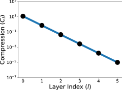
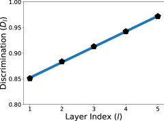
(a) $6$-layer linear network

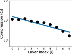
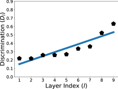
(b) $10$-layer nonlinear network

Figure 4: Progressive feature compression and discrimination on both linear and nonlinear networks. We plot the feature compression and discrimination metrics defined in (8) at each layer for both the linear network (top row) and nonlinear network (bottom row). We train both networks using a nearly orthogonal dataset as described in 1, initializing the network weights satisfying (18), with an initialization scale of $\xi=0.3$. We train both networks via gradient descent until convergence. In each figure, the $x$-axis denotes the number of layers from shallow to deep. In the left figures, the $y$-axis denotes the compression measure $C_{l}$ in the logarithmic scale; In the right figures, the $y$-axis denotes the discrimination measure $D_{l}$. More experimental details can be found in Section 5.2.2.

Implicit bias of GD.

Since the DLN in Problem (3) is over-parameterized, it has infinitely many solutions satisfying $\bm{W}_{L:1}\bm{X}=\bm{Y}$. However, GD for training networks typically has an implicit bias towards certain solutions with benign properties [4, 45, 61, 82, 100, 94]. Specifically, previous work has demonstrated that, with assumptions concerning network initialization and the dataset, gradient flow tends to favor solutions with minimum norms and balanced weights; see, e.g., [82, 22, 3, 30]. Recent studies have also revealed that GD primarily updates a minimal invariant subspace of the weight matrices, thereby preserving approximate low-rankness of the weights across all layers [49, 117]. Based on these observations, we assume that the trained weights $\bm{\Theta}$ satisfy the following benign properties to investigate how trained deep networks hierarchically transform input data into labels.

Assumption 2.

For an $L$-layer DLN with weights $\bm{\Theta}=\{\bm{W}_{l}\}_{l=1}^{L}$ described in (2) with $d_{l}=d>2K$ for all $l\in[L-1]$, the weights $\bm{\Theta}$ satisfy
(i) Minimum-norm solution:

$$\bm{W}_{L:1}=\bm{Y}(\bm{X}^{T}\bm{X})^{-1}\bm{X}^{T}.$$ (10)

(ii) $\delta$-Balancedness: There exists a constant $\delta>0$ such that

$$\bm{W}_{l+1}^{T}\bm{W}_{l+1}=\bm{W}_{l}\bm{W}_{l}^{T},\forall l\in[L-2],\ \|\bm{W}_{L}^{T}\bm{W}_{L}-\bm{W}_{L-1}\bm{W}_{L-1}^{T}\|_{F}\leq\delta.$$ (11)

(iii) $\varepsilon$-Approximate low-rank weights: There exist positive constants $\varepsilon\in(0,1)$ and $\rho\in[0,\varepsilon)$ such that for all $l\in[L-1]$,

$$\varepsilon-\rho\leq\sigma_{i}(\bm{W}_{l})\leq\varepsilon,\ \forall i=K+1,\dots,d-K.$$ (12)

We defer the discussion on 2 to Section 3.2, where we provide both theoretical and empirical evidence to support it. Building upon the above assumptions, we now present our main theorem concerning hierarchical representations in terms of feature compression and discrimination.

Theorem 1.

Consider a $K$-class classification problem on the training data $(\bm{X},\bm{Y})\in\mathbb{R}^{d\times N}\times\mathbb{R}^{K\times N}$, where the matrix $\bm{X}$ satisfies Assumption 1 with parameter $\theta$. Suppose that we train an $L$-layer DLN with weights $\bm{\Theta}=\left\{\bm{W}_{l}\right\}_{l=1}^{L}$ such that $\bm{\Theta}$ satisfies Assumption 2, with the parameters $(\delta,\rho,\varepsilon)$ of weight balancedness and low-rankness satisfying

$$\delta\leq\min\left\{\frac{(2n)^{1/L}}{30L^{2}},\frac{n^{1/L}}{128\sqrt{K}},\frac{1}{16\sqrt{K}}\right\},\ \varepsilon\leq\min\left\{\frac{n^{\frac{1}{2L}}}{4},1\right\},\ \rho\leq\frac{\varepsilon}{2L\sqrt{n}}.$$ (13)

(i) Progressive within-class feature compression: It holds that

$$\frac{c\varepsilon^{2}}{\kappa(2n)^{1/L}}\leq\frac{C_{1}}{C_{0}}\leq\frac{2\kappa\varepsilon^{2}}{c(n/2)^{1/L}},$$ (14)

$$\frac{c\varepsilon^{2}}{\kappa(2n)^{1/L}}\leq\frac{C_{l+1}}{C_{l}}\leq\frac{\kappa\varepsilon^{2}}{c(n/2)^{1/L}},\ \forall l\in[L-2],$$ (15)

where

$$c=\frac{(n-3)K-1}{(n-1)K+1},\ \kappa=\frac{1+n^{-\Omega(1)}}{1-n^{-\Omega(1)}}.$$

(ii) Progressive between-class feature discrimination: For all $l\in[L-1]$, we have

$$D_{l}\geq 1-32\left(\theta+4\delta\right)\left(2-\frac{l+1}{L}\right)-n^{-\Omega(1)}.$$ (16)

We defer the detailed proof to Appendix B. As we discussed in Section 1, numerous empirical studies have been conducted to explore the feature structures of intermediate and final layers in deep networks, particularly concerning feature compression and discrimination; see, e.g., [1, 7, 17, 25, 34, 42, 51, 47, 79, 92, 91, 119]. However, there remains a scarcity of theoretical analysis to elucidate their observations. Despite the acknowledged limitations of DLNs, our work takes the first step towards rigorously developing a unified framework to quantify feature compression and discrimination across different layers. Specifically, 1 shows that, given input data satisfying 1, for a trained DLN with weights satisfying 2, features within the same class are compressed at a geometric rate on the order of ${\varepsilon^{2}}/{n^{1/L}}$ when $n$ is sufficiently large, while the features between classes are discriminated at a linear rate on the order of $1/L$ across layers. These findings are strongly supported by our empirical results in Figure 4 (top figures), and also appear on nonlinear networks as shown in Figure 4 (bottom figures). In the following, we discuss the implications of our main result.

From linear to nonlinear networks.

Although our result is rooted in DLNs, it provides valuable insights into the feature evolution in nonlinear networks. Specifically, the linear separability of features learned by initial layers in nonlinear networks (see Figure 1) allows subsequent layers to be effectively replaced by linear counterparts for compressing within-class features and discriminating between-class features (see Figure 5). Therefore, studying DLNs helps us understand the role of the nonlinear layers after the initial layers in nonlinear networks for learning features. This understanding also sheds light on the pattern where within-class features compress at a geometric rate and between-class features discriminate at a linear rate in nonlinear networks approximately, as illustrated in Figure 4 (bottom figures). A natural direction is to extend our current analysis framework to nonlinear networks, especially homogeneous neural networks [74].

Neural collapse beyond the unconstrained feature model.

One important implication of our result is that it addresses an open problem about NC. Specifically, almost all existing works assume the unconstrained feature model [80, 87] (or layer-peeled model [37, 59]) to analyze the NC phenomenon, where the last-layer features of the deep network are treated as free optimization variables to simplify the interactions across layers; see, e.g., [120, 59, 110, 123, 118, 121, 76]. However, a major drawback of this model is that it overlooks the hierarchical structures of deep networks and intrinsic structures of the input data. In this work, we address this issue without assuming the unconstrained feature model. Specifically, according to 1, when a linear network is deep enough and trained on nearly orthogonal data, the last-layer features within the same class concentrate around their class means, while the last-layer features from different classes are nearly orthogonal to each other. This directly implies the last-layer features exhibit variability collapse and convergence to simplex equiangular right frame approximately after centralization.

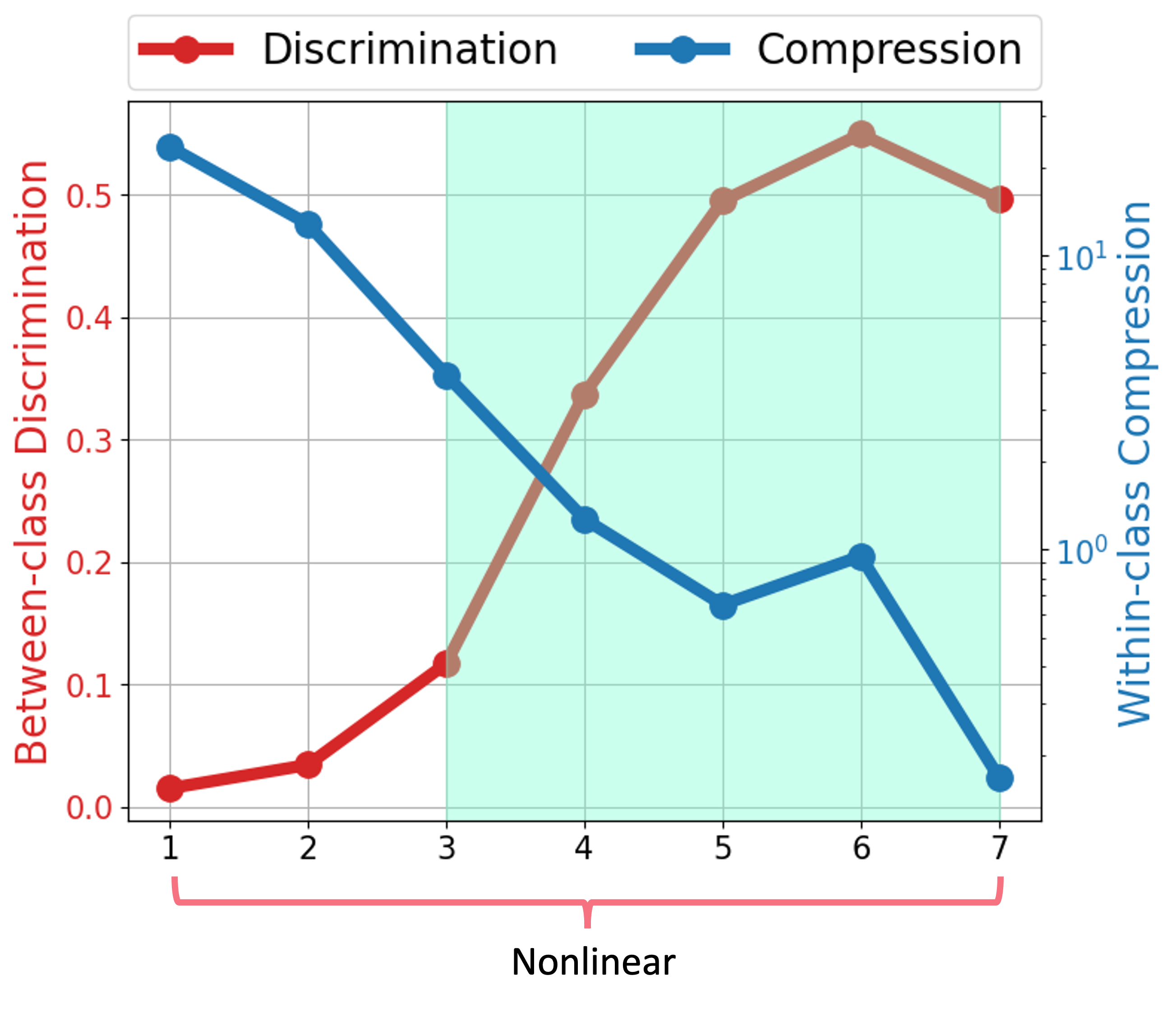
(a) A 7-layer MLP network with ReLU

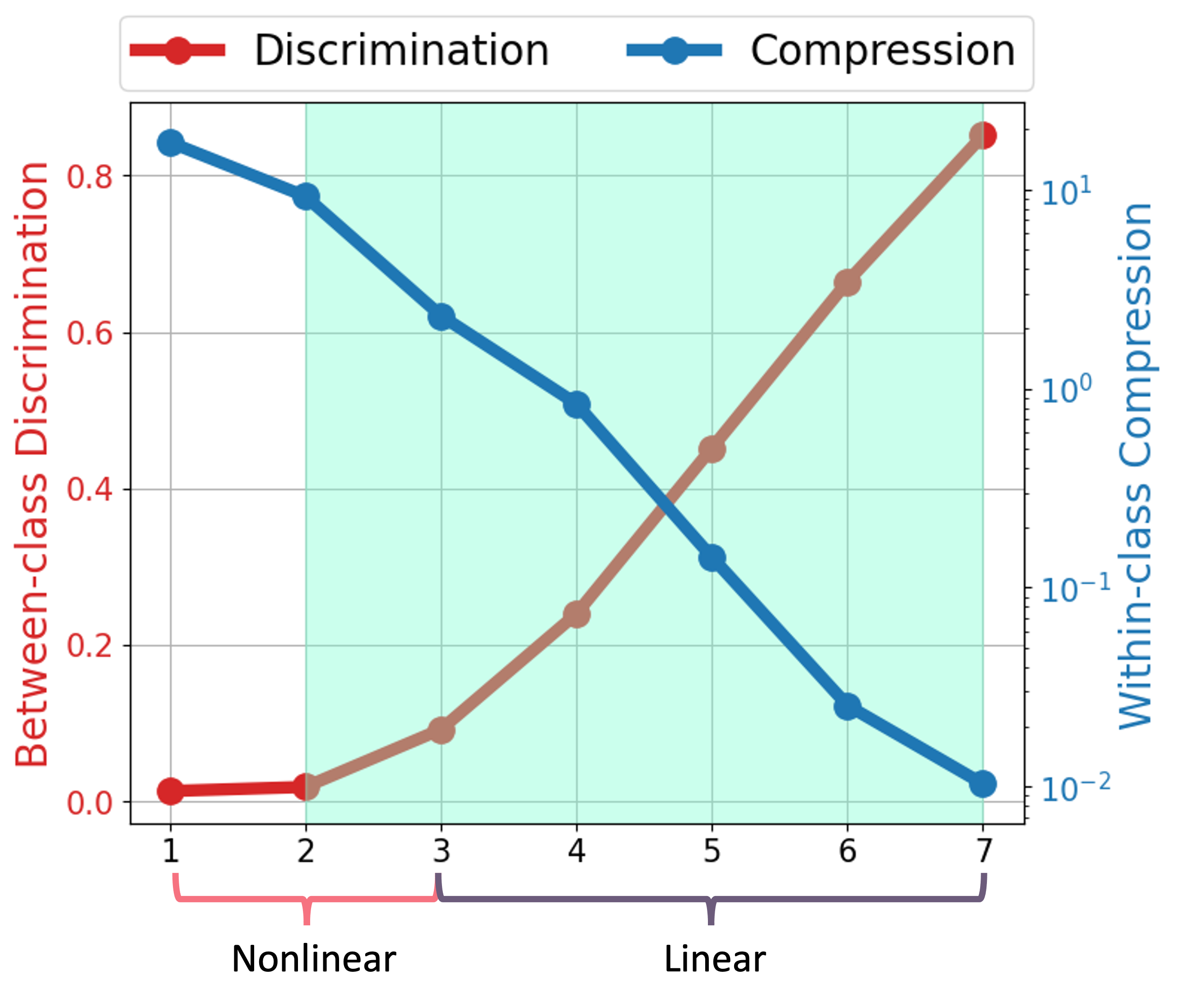
(b) A 7-layer hybrid network

Figure 5: Within-class compression and between-class discrimination of features of two 7-layer networks. We use the same setup as in Figure 1 and plot the metrics of within-class compression and between-class discrimination (see Definition 1) of the two networks across layers after training, respectively. More experimental details are deferred to Section 5.1.1.

Guidance on network architecture design.

Progressive feature compression and discrimination in 1 provide guiding principles for network architecture design. Specfically, according to (14), (15), and (16), the features are more compressed within the same class and more discriminated between different classes, improving the separability of input data as the depth of networks increases. This is also supported by our experiments in Figure 12. This indicates that the networks should be deep enough for effective data separation in classification problems. However, it is worth noting that the belief that deeper networks are better is not always true. Indeed, it becomes increasingly challenging to train a neural network as it gets deeper, especially for DLNs [40]. Moreover, over-compressed features may degrade the out-of-distribution performance of deep networks as shown in [79]. This, together with our result, indicates that neural networks should not be too deep for improved out-of-distribution generalization performance.

Understanding projection heads for transfer learning.

In contrastive learning [21, 20], a successful empirical approach to improving transfer learning performance in downstream tasks involves the use of projection heads [75]. These projection heads, typically consisting of one or several MLP layers, are added between the feature extractor and the final classifier layers during pre-training. For downstream tasks, the projection head is discarded and only the features learned by the feature extractor are utilized for transfer learning. Recent works [75, 63, 43, 112] have established an empirical correlation between the degree of feature collapse during pre-training and downstream performance: less feature collapse leads to more transferable models. However, it remains unclear why features prior to projection heads exhibit less collapse and greater transferability. Our study addresses this question and offers a theoretical insight into the utilization of projection heads. According to 1, it becomes apparent that features from the final layers tend to be more collapsed than the features before the projection head. This, together with the empirical correlation between feature collapse and transferability, implies that leveraging features before projection heads improves transferability. This is also supported by our experimental results in Section 5.3.2. Moreover, the progressive compression pattern in 1 also provides insight into the phenomenon studied in [115], which suggests that deeper layers in a neural network become excessively specialized for the pre-training task, consequently limiting their effectiveness in transfer learning.

3.2 Discussions on 2

In this subsection, we justify the properties imposed on the trained network weights as outlined in 2, drawing insights from both our theoretical and experimental findings. It is important to emphasize that the solution described in 2 represents just one of infinitely many globally optimal solutions for Problem (3). Nevertheless, because of the implicit bias in GD training dynamics, GD iterations with proper initialization almost always converge to the desired solutions outlined in 2. In the subsequent discussion, we will delve into this phenomenon in greater depth.

GD with orthogonal initialization.

We consider training a DLN for solving Problem (3) by GD, i.e., for all $l\in[L]$,

$$\bm{W}_{l}{(t+1)}=\bm{W}_{l}{(t)}-\eta\frac{\partial\ell(\bm{\Theta}{(t)})}{\partial\bm{W}_{l}},\ t\geq 0.$$ (17)

Notably, when the learning rate is infinitesimally small, i.e., $\eta\to 0$, GD in (17) reduces to gradient flow. Moreover, we initialize the weight matrices $\bm{W}_{l}$ for all $l\in[L]$ using $\xi$-scaled orthogonal matrices for a constant $\xi>0$, i.e.,

$$\bm{W}_{l}{(0)^{T}}\bm{W}_{l}{(0)}=\xi^{2}\bm{I}_{d},\forall l\in[L-1],\quad\bm{W}_{L}{(0)}=\left[\xi\bm{U}\ \bm{0}\right],$$ (18)

where $\bm{U}\in\mathcal{O}^{K}$. It is worth noting that orthogonal initialization is widely used to train deep networks, which can speed up the convergence of GD; see, e.g., PSG [89], SMG [95], XBSD⁺ [111], HXP [53].

Theoretical justification of 2.

Theoretically, we can prove the conditions outlined in Assumption 2 when the gradient flow is trained on a square and orthogonal data matrix using the results in [3, 117].

Proposition 1.

Suppose that the data matrix $\bm{X}\in\mathbb{R}^{d\times N}$ is square, i.e., $d=N$, and satisfies Assumption 1 with $\theta=0$. Suppose in addition that we apply GD (17) to solve Problem (3) with $\eta\to 0$ and the initialization in (18). If GD converges to a global optimal solution, then (10), (11), and (12) hold with $\delta=\xi^{2}\sqrt{d-K}$, $\varepsilon=\xi$, and $\rho=0$.

The proof of this proposition is deferred to Section B.5. Although we can only prove 2 in this restrictive setting, it actually holds in more general settings. We substantiate this claim by drawing support from empirical evidence and existing findings in the literature, as elaborated in the following.

Empirical justifications of 2.

Here, we run GD (17) using the initiation (18) on nearly orthogonal data satisfying Assumption 1. We refer the reader to Section 5.2 for the experimental setup. After training, we plot the metrics of minimum norm residual, balancedness residual, and variance of singular values (see the legends in Figure 6) against depth (resp. width) in Figure 6(a) (resp. Figure 6(b)). It is observed that the magnitudes of these metrics are very small for different depths and widths of neural networks. This indicates that Assumption 2 approximately holds for GD in a broader setting.

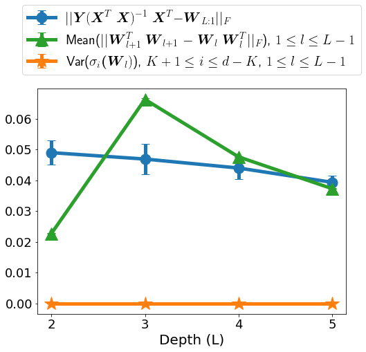
(a) Fix width $d=400$, change depth $L$

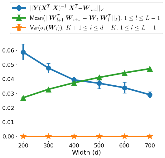
(b) Fix depth $L=5$, change width $d$

Figure 6: 2 holds approximately among different network configurations. We train DLNs using the orthogonal initialization with varying widths and depths. For each network width $d$ and depth $L$, we show the minimum-norm residual, the average weight balancedness residual of all weights, and the variance of the singular values of all weights (see (5.2.1) for details) for the DLNs that have been trained until convergence. Each data point represents the mean value of 10 runs with different random seeds. Here, we plot these metrics in (a) with fixed network width $d$ and varying depth $L$ and (b) with fixed network depth $L=5$ and varying network width $d$. More experimental details are deferred to Section 5.2.1.

Prior arts on implicit bias support 2.

Moreover, 2 is also well supported by many related results in the literature.

• Minimum-norm solutions and balanced weights. It has been extensively studied in the literature that GD with proper initialization converges to minimum-norm and balanced solutions, especially in the setting of gradient flow [3, 22, 30, 82]. Specifically, [30, 3] proved that for linear networks, the iterates of gradient flow satisfy

  $$\frac{d}{dt}\left(\bm{W}_{l}(t)\bm{W}_{l}(t)^{T}-\bm{W}_{l+1}(t)^{T}\bm{W}_{l+1}(t)\right)=\bm{0},\ \forall l\in[L-1],$$ (19)

  where $t$ denotes a continuous time index. This, together with (18), implies that (11) holds with $\delta=\xi\sqrt{d-K}$. Moreover, using the result in [82], if we initialize the weights of two-layer networks as in (18) with $\bm{W}_{2}(0)\bm{W}_{1}(0)\in\mathrm{span}(\bm{X})$, gradient flow always yields the minimum-norm solution upon convergence. However, the conditions (10) and (11) are rarely studied in the context of GD for training deep networks. In this context, we empirically verify these two conditions as shown in Figure 6 under different network configurations.

• Approximate low-rankness of the weights. Recently, numerous studies have demonstrated that GD exhibits a bias towards low-rank weights [4, 45, 117, 68]. In particular, [117, 68] showed that when the input data $\bm{X}$ is orthonormal, learning dynamics of GD for DLNs in (17), with the initialization in (18), only updates an invariant subspace of dimension $2K$ for each weight matrix across all layers, where the invariant subspace is spanned by the singular vectors associated with the $K$-largest and $K$-smallest singular values, and the rest singular values remain unchanged. More experimental demonstration can be found in Appendix C.

4 Relationship to Prior Arts

In this section, we discuss the relationship between our results and prior works on the empirical and theoretical study of deep networks.

Hierarchical feature learning in deep networks.

Deep networks, organized in hierarchical layers, can perform effective and automatic feature learning [10], where the layers learn useful representations of the data. To better understand hierarchical feature learning, plenty of studies have been conducted to investigate the structures of features learned at intermediate layers. One line of these works is to investigate the neural collapse (NC) properties at intermediate layers. For example, [105] extended the study of neural collapse to three-layer nonlinear networks with the MSE loss, showing that the features of each layer exhibit neural collapse. [32] generalized the study of neural collapse for DLNs with imbalanced training data, and they draw a similar conclusion as [105] that the features of each layer are collapsed. However, these results are based on the unconstrained feature model and thus cannot capture the input-output relationship of the neural networks. Moreover, the conclusion they draw on the collapse of intermediate features is far from what we observe in practice. Indeed, it is observed on both linear and nonlinear networks in Figure 4 that the intermediate features are progressively compressed across layers rather than exactly collapsing to their means for each layer. In comparison, under the assumption that the input $\bm{X}$ is nearly orthogonal in 1, our result characterizes the progressive compression and discrimination phenomenon to capture the training phenomena on practical networks as demonstrated in Figure 4.

On the other hand, another line of work [116, 24, 27, 81, 114] argues that deep networks prevent within-class feature compression while promoting between-class feature discrimination, contrasting with our study where features are compressed across layers. Such a difference comes from the choices of loss functions. In our work, we focused on the study of the commonly used MSE loss, with the goal of understanding a prevalent phenomenon in classical training of deep networks. It has been empirically shown that increasing feature compression is beneficial for improving in distribution generalization and robustness [87, 75, 17, 51, 19]. In comparison, [116] introduced a new maximum coding rate reduction loss that is intentionally designed to prevent feature compression.

Distinction from the neural tangent kernel: feature learning.

There has been a rich line of work that studies mathematical insights into deep networks in the regime where the width of a network is sufficiently large. In the infinite-width limit, it has been demonstrated that neural networks converge to a solution to a kernel least squares problem [58]. This is referred to as the neural tangent kernel (NTK), which serves as an important theoretical tool in understanding the convergence [11, 29, 33] and generalization [8, 5] of neural networks in the kernel regime. However, its effectiveness is limited when it comes to understanding hierarchical structure and justifying the advantages of deep architectures in neural networks. For example, recent works [9, 18, 31, 78] have identified sets of functions that deep architectures can efficiently learn, yet kernel methods fall short in learning these functions in theory. In comparison, our work offers insights into understanding hierarchical representations of neural networks in terms of feature compression and discrimination from shallow to deep layers.

Learning dynamics and implicit bias of GD for training deep networks.

Our main result in 1 is based on 2 for the trained weights. As discussed in Section 3.2, 2 holds as a consequence of results in recent works on analyzing the learning dynamics and implicit bias of gradient flow or GD in training deep networks. We briefly review the related results as follows. For training DLNs, [2] established linear convergence of GD based upon whitened data and with a similar setup to ours. For Gaussian initialization, [29] showed that GD also converges globally at a linear rate when the width of hidden layers is larger than the depth, whereas [53] demonstrated the advantage of orthogonal initialization over random initialization by showing that linear convergence of GD with orthogonal initialization is independent of the depth. More recent developments can be found in [41, 86, 93] for studying GD dynamics. On the other hand, another line of works focused on studying gradient flow for learning DLNs due to its simplicity [16, 35, 82, 106, 16], by analyzing its convergence behavior.

Numerous studies have shown that the effectiveness of deep learning is partially due to the implicit bias of its learning dynamics, which favors some particular solutions that generalize exceptionally well without overfitting in the over-parameterized setting [13, 49, 83]. To gain insight into the implicit bias of GD for training deep networks, a line of recent work has shown that GD tends to learn simple functions [26, 45, 60, 67, 100, 108]. For instance, some studies have shown that GD is biased towards max-margin solutions in linear networks trained for binary classification via separable data [94, 67]. In addition to the simplicity bias, another line of work showed that deep networks trained by GD exhibit a bias towards low-rank solutions [45, 49, 117]. The works [41, 4] demonstrated that adding depth to a matrix factorization enhances an implicit tendency towards low-rank solutions, leading to more accurate recovery.

5 Experimental Results

In this section, we conduct various numerical experiments to validate our assumptions, verify the theoretical results, and investigate the implications of our results on both synthetic and real data sets. All of our experiments are conducted on a PC with 8GB memory and Intel(R) Core i5 1.4GHz CPU, except for those involving large datasets such as CIFAR and FashionMNIST, which are conducted on a computer server equipped with NVIDIA A40 GPUs. Our codes are implemented in Python and are available at https://github.com/Heimine/PNC_DLN. Throughout this section, we will repeatedly use multilayer perception (MLP) networks, where each layer of MLP networks consists of a linear layer and a batch norm layer [57] followed by ReLU activation.

The remaining sections are organized as follows: In Section 5.1, we provide detailed experimental setups for the results discussed in Section 1 and shown in Figures 5, 7, and 8. In Section 5.2, we provide experimental results to support 1 in Section 3 and validate Assumption 2 discussed in Section 3.2. Finally, we empirically explore the implications of our results in Section 5.3 beyond our assumptions.

5.1 Significance of Studying DLNs in Feature Learning

(a) A 7-layer MLP network with ReLU

(b) A 7-layer hybrid network

Figure 7: Accuracy and numerical rank of two 7-layer networks before training. We use the same setup as in Figures 1 and 5 but instead plot the numerical rank and training accuracy of the two networks across layers before training.

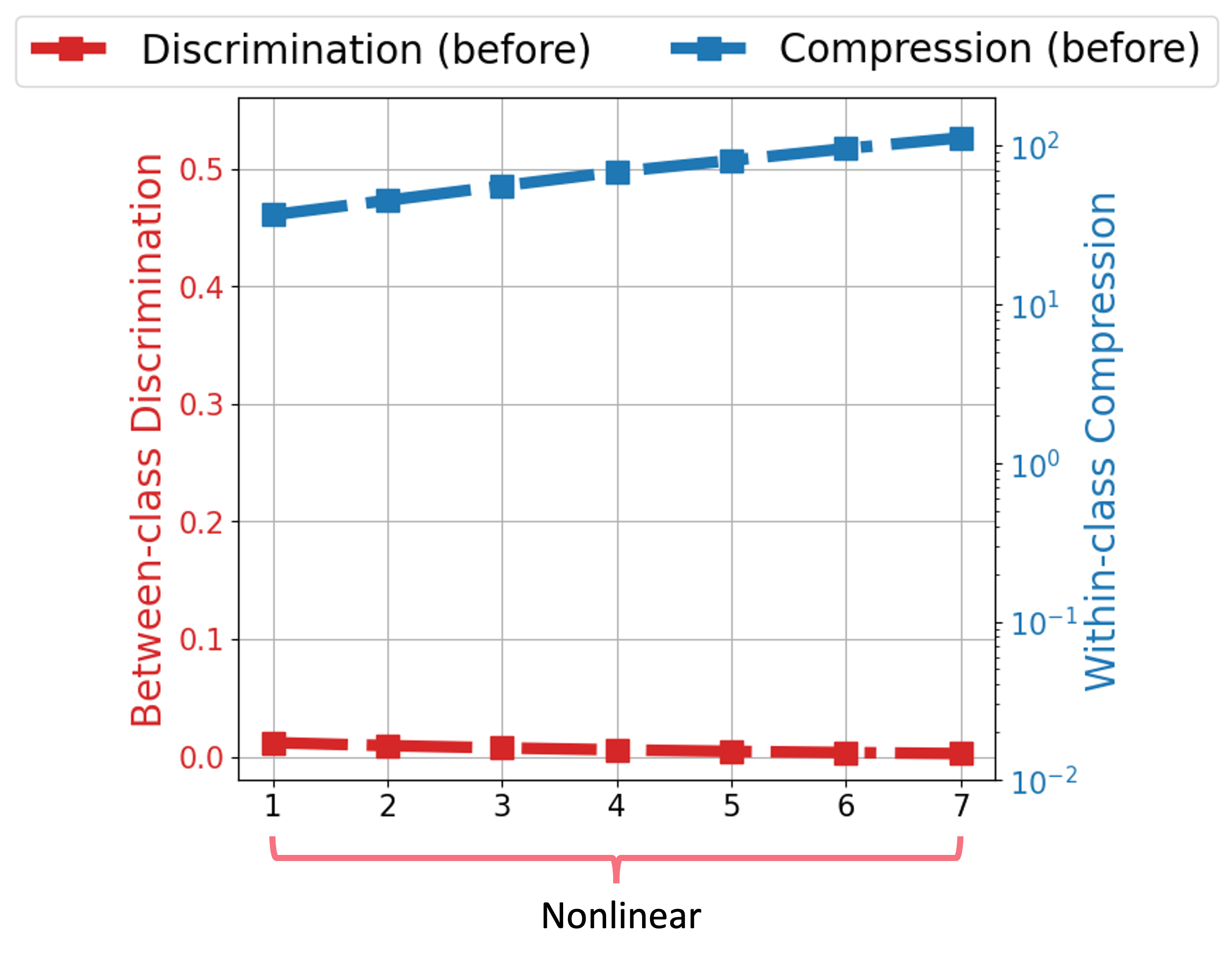
(a) A 7-layer MLP network with ReLU

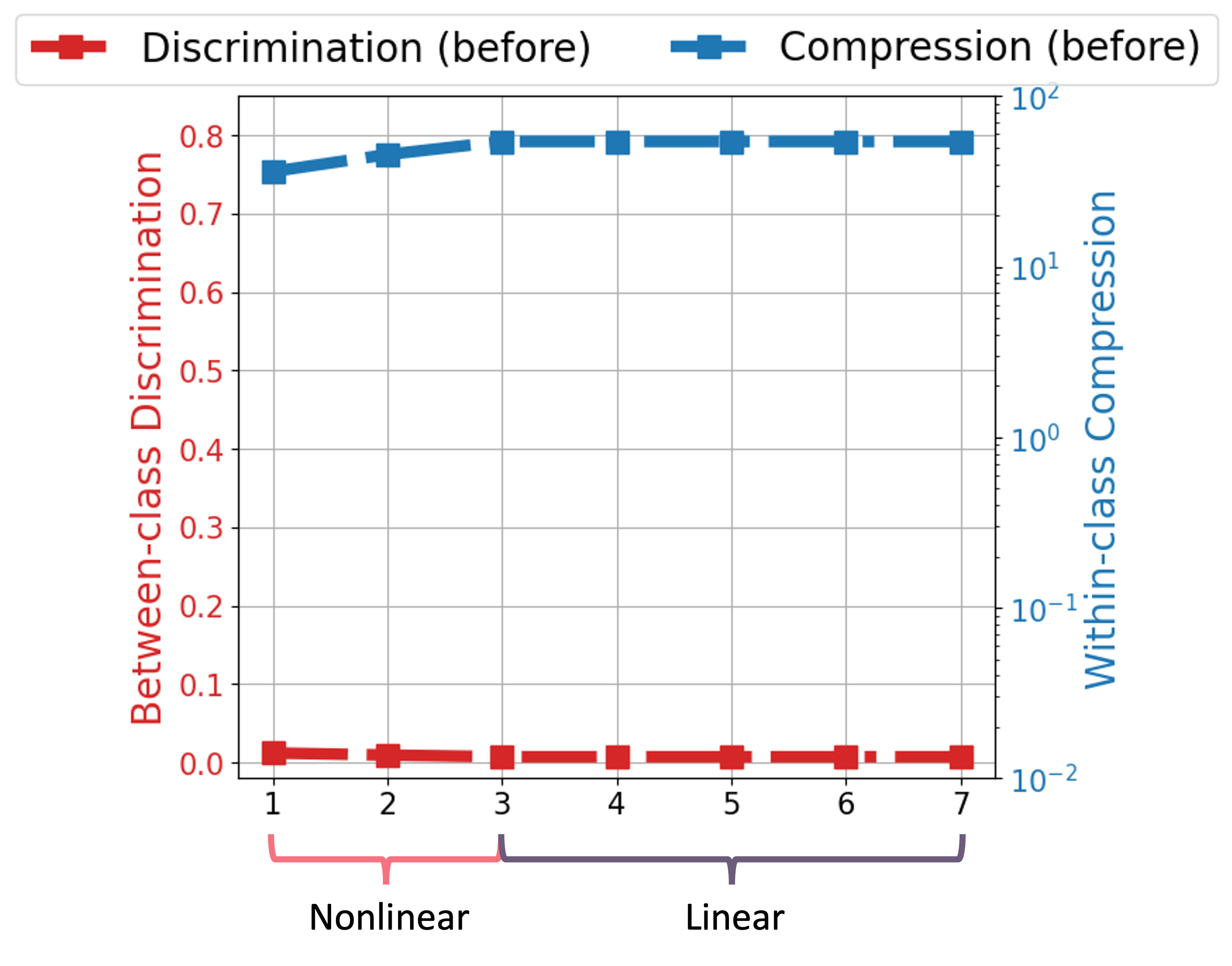
(b) A 7-layer hybrid network

Figure 8: Within-class compression and Between-class discrimination of two 7-layer networks before training. We use the same setup as in Figure 1 and Figure 5 but instead plot the compression and discrimination statistics of the two networks across layers before training.

In this subsection, our goal is to empirically demonstrate the significance of studying DLNs in feature learning as discussed in Section 1. To achieve this, we investigate (i) the roles of linear layers and MLP layers at deep layers in feature learning and (ii) the importance of the depth of DLNs for generalization performance.

5.1.1 Linear Layers Mimic Deep Layers in MLPs for Feature Learning

In this subsection, we study the roles of linear layers and MLP layers at deep layers in feature learning. To begin, we provide the experimental setup for our experiments.

Network architectures.

In these experiments, we construct two 7-layer networks: (a) a nonlinear MLP network and (b) a hybrid network formed by a 3-layer MLP followed by a 4-layer linear network. We set the hidden dimension $d=1024$ for all linear layers.

Training dataset and training methods.

We employ the SGD optimizer to train the networks by minimizing the MSE loss on the CIFAR-10 dataset [64]. For the settings of the SGD optimizer, we use a momentum of 0.9, a weight decay of $10^{-4}$, and a dynamically adaptive learning rate ranging from $10^{-3}$ to $10^{-5}$, modulated by a CosineAnnealing learning rate scheduler as detailed in [72]. We use the orthogonal initialization in (18) with $\xi=0.1$ to initialize the network weights. The neural networks are trained for 200 epochs with a batch size of 128.

Experiments and observations.

Now, we elaborate on the tasks conducted in Figures 1, 2, 5, 7, and 8 and draw conclusions from our observations.

• In Figure 1 (resp. Figure 7), we plot the numerical rank and training accuracy of the features against the layer index after training (resp. before training). Here, the numerical rank of a matrix is defined as the number of its singular values whose sum collectively accounts for more than 95% of its nuclear norm. In terms of training accuracy, we add a linear classification layer to a given layer $l$ of the neural network and train this added layer using the cross-entropy loss to compute the classification accuracy. It is observed in Figure 1 that the training accuracy rapidly increases in the initial layers and nearly saturates in the deep layers, whereas the numerical rank increases in the initial layers and then decreases in the deep layers progressively in the trained networks. This observation suggests that the initial layers of a network create linearly separable features that can achieve accurate classification, while the subsequent layers further compress these features progressively.

• In Figure 2, we employ a 2D UMAP plot [77] with the default settings in the UMAP Python package to visualize the evolution of features from shallow to deep layers. It is observed that in the first layer, features do not exhibit obvious structures in terms of feature compression and discrimination; the features from the same class are more and more compressed, while the features from different classes become more and more separable from layer 2 to layer 4; this within-class compression and between-class discrimination pattern is strengthened from layer 4 to layer 6. This visualization demonstrates that features in the same class are compressed, while the features from different classes are discriminated progressively.

• In Figure 5 (resp. Figure 8), we plot the metrics of within-class feature compression $C_{l}$ and between-class feature discrimination $D_{l}$ defined in 1 against the layer index after training (resp. before training). According to Figure 5, we observe a consistent trend of decreasing $C_{l}$ and increasing $D_{l}$ against the layer index after training for both networks, albeit the hybrid network exhibits a smoother transition in $C_{l}$ and $D_{l}$ compared to the fully nonlinear network. This observation supports our result in 1.

The role of linear layers in feature learning.

Comparing Figure 1(a) to Figure 1(b) and Figure 5(a) to Figure 5(b), we conlcude that linear players play the same role as MLP layers in the deep layers of nonlinear networks in feature learning, compressing within-class features and discriminating between-class features progressively. Intuitively, this is because the representations from the initial layers are already linearly separable, we can replace the deeper nonlinear layers with DLNs to achieve the same functionality without sacrificing the training performance. Moreover, comparing the results after training (Figures 1 and 5) with those before training (Figures 7 and 8), we conclude that training neural networks using SGD learn feature representations beyond NTK regime. This finding aligns with the results in recent works [12, 31].

5.1.2 Effects of Depth in Linear Layers for Improving Generalization

In this subsection, we study the impact of depth of deep networks on generalization performance. To begin, we provide the experimental setup for our experiments.

Network architectures.

We consider a 2-layer MLP network as our base network and construct networks of varying depths from 3 to 9 by adding linear or MLP layers to this base network. We use the PyTorch default initialization [55] to initiate all weights.

Training dataset and training methods.

We train these networks on the FashionMNIST [113] and CIFAR-10 [64] datasets, using the same training approach in Section 5.1.1, except that the initial learning rate is set as $10^{-2}$. We use $5$ different random seeds to initialize the network weights and report the average test accuracy.

Experiments and observations.

After training, we report the average test accuracy throughout training against the number of layers of constructed networks in Figure 3. Notably, we observe a consistent improvement in test accuracy as the networks grow deeper, regardless of whether the added layers are linear or MLP layers. This observation provides further evidence for the resemblance between DLNs and the deeper layers in MLPs. Additionally, it also shows that DLNs can benefit from increased depth, similar to their counterparts in traditional nonlinear networks.

5.2 Experimental Verification of 2 and 1

In this subsection, we conduct numerical experiments to verify our assumptions and theorem presented in Section 3. Unless otherwise specified, we use the following experimental setup.

Network architectures.

We study DLNs and MLPs with ReLU activation with different widths and depths specified in each figure.

Training dataset.

In all experiments, we fix the number of classes $K=3$ and the number of training samples $N=30$, with varying hidden dimensions $d\geq N$ as specified in each figure. To generate input data $\bm{X}\in\mathbb{R}^{d\times N}$ that satisfies Assumption 1, we first generate a matrix $\bm{A}\in\mathbb{R}^{d\times N}$ with entries i.i.d. sampled from the standard normal distribution and a matrix $\bm{B}\in\mathbb{R}^{d\times N}$ with entries i.i.d. sampled from the uniform distribution on $[0,1]$. Then, we apply a compact SVD to $\bm{A}$ and set ${\bm{X}}_{0}\in\mathbb{R}^{d\times N}$ as the left singular matrix. Next, we obtain a matrix $\bm{N}$ by normalizing $\bm{B}$ such that its Frobenious norm is 1. Finally, we generate $\bm{X}$ via $\bm{X}={\bm{X}}_{0}+\bm{N}$ such that $\bm{X}$ is nearly orthogonal satisfying 1.

Training method and weight initialization.

Unless otherwise specified, we train networks using full batch GD in (17), with a fixed learning rate $\eta=0.1$. We use orthogonal weight initialization as described in (18) with varying initialization scaling $\xi$. This initialization ensures that the weights at initialization meet the condition (11).

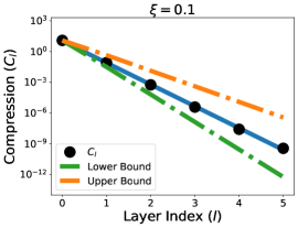
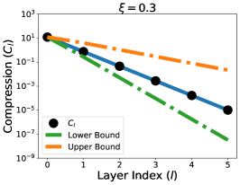
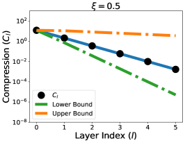
(a) The metric of within-class compression $C_{l}$

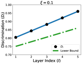
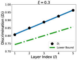
(b) The metric of between-class discrimination $D_{l}$

Figure 9: Visualization of the metrics of within-class compression $C_{l}$ and between-class discrimination across layers. We train 6-layer DLNs with $\xi=0.1,0.3,0.5$, respectively. In the top figures, we plot the metric of within-class compression $C_{l}$ along with the corresponding theoretical upper and lower bounds given in (15). In the bottom figures, we plot the metric of between-class discrimination given in (16).

5.2.1 Experiments for Verifying 2

In this subsection, we conduct experiments to verify 2 and corroborate the discussions in Section 3.2 based on the above experimental setup. Specifically, we train DLNs using orthogonal initialization in (18) with $\xi=0.1$ for various network depths and widths. Given a DLN, we train it 10 times with different random seeds. In each run, we terminate training once the training loss is less than $10^{-11}$. We plot the following metrics over 10 runs against depth and width in Figure 6(a) and Figure 6(b), respectively:

$$\text{minimum-norm residual:}\quad||\bm{Y}(\bm{X}^{T}\bm{X})^{-1}\bm{X}^{T}-\bm{W}_{L:1}||_{F},$$

$$\text{averaged balancedness:}\quad\frac{1}{L-1}\sum_{l=1}^{L-1}||\bm{W}_{l+1}^{T}\bm{W}_{l+1}-\bm{W}_{l}\bm{W}_{l}^{T}||_{F},$$ (20)

$$\text{variance of singular values of all weights:}\ \frac{1}{(L-1)(d-2K)}\sum_{l=1}^{L-1}\sum_{i=K+1}^{d-K}\left(\sigma_{i}(\bm{W}_{l})-\mu\right)^{2},$$

where $\mu=\frac{1}{(L-1)(d-2K)}\sum_{l=1}^{L-1}\sum_{i=K+1}^{d-K}\sigma_{i}(\bm{W}_{l})$. It can be observed from Figure 6 that the weights of a DLN with different depths and widths trained under our settings approximately satisfy 2. This supports our discussions in Section 3.2.

5.2.2 Experiments for Verifying 1

Now, we conduct experiments to validate 1. Specifically, we train 6-layer DLNs using GD with varying initialization scales $\xi=0.1,0.3,0.5$, respectively. Then, we plot the metrics of within-class compression $C_{l}$ and between-class discrimination $D_{l}$ against layer index in Figure 9(a) and Figure 9(b), respectively. It is observed that the feature compression metric $C_{l}$ decreases exponentially, while the feature discrimination metric $D_{l}$ increases linearly w.r.t. the layer index. In the top row of Figure 9, the solid blue line is plotted by fitting the values of $C_{l}$ at different layers, and the green and orange dash-dotted lines are plotted according to the lower and upper bounds in (15), respectively. We can observe that the solid blue line is tightly sandwiched between the green and orange dash-dotted lines. This indicates that (14) and (15) provide a valid and tight bound on the decay rate of the feature compression metric. According to the bottom row of Figure 9, we conclude that (16) provides a valid bound on the growth rate of the feature discrimination metric.

Moreover, we respectively train 9-layer DLN and MLP networks with hidden dimension $d=50$ via GD with an initialization scale $\xi=0.3$. In Figure 4, we plot the feature compression and discrimination metrics on both DLN and MLP networks, respectively. We can observe that exponential decay of feature compression and linear increasing of feature discrimination holds exactly on DLNs, and approximately on nonlinear networks.

5.3 Exploratory Experiments

5.3.1 Empirical Results Beyond Theory

In this subsection, we conduct exploratory experiments to demonstrate the universality of our result. Unless otherwise specified, we use the experimental setup outlined at the beginning in Section 5.2 in these experiments. Here are our observed findings:

• Progressive feature compression and discrimination in nonlinear deep networks. We train 8-layer and 16-layer MLP networks, respectively. After training, we plot the metrics of feature compression and discrimination defined in (1) in Figure 10. It is observed that the feature compression metric $C_{l}$ decays at an approximate geometric rate in nonlinear networks, while the feature discrimination metric $D_{l}$ increases at an approximate linear rate. Additionally, it is worth mentioning that a similar “law of separation” phenomenon has been reported in [51, 75] on nonlinear networks, but their results are based upon a different metric of data separation.

• Progressive feature compression and discrimination on DLNs with generic initialization. In most of our experiments and discussion in Section 3.2, we mainly focused on orthogonal initialization, which simplifies our analysis due to induced weight balancedness across layers. To demonstrate the generality of our results, we also test the default initialization in the PyTorch package and train the DLN. As shown in Figure 11, we can observe that the compression metric $C_{l}$ decays from shallow to deep layers at an approximate geometric rate with different network depth $L$. Additionally, the discrimination metric $D_{l}$ increases at an approximate linear rate.

• Progressive feature compression on real datasets. We train a hybrid network on FashionMNIST and CIFAR datasets using the network architectures and training methods in Section 5.1.2 and plot the metric of within-class compression against layer index in Figure 12. Although we use real data sets and PyTorch default initialization, we can still observe that the within-class compression metric $C_{l}$ decays progressively at an approximate geometric rate. This further demonstrates the universality of our studied phenomenon. Moreover, the results in Figure 12 also illustrate the role of depth, where the decay rates are approximately the same across all settings, and thus deeper networks lead to more feature compression.

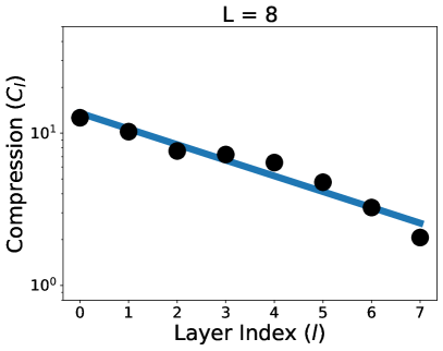
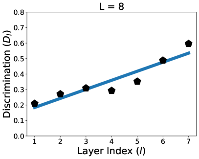
(a) 8-layer MLP.

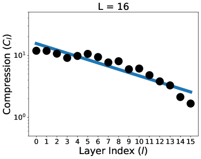
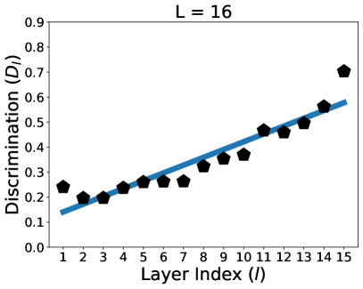
(b) 16-layer MLP.

Figure 10: Progressive feature compression and discrimination on nonlinear networks. We train MLP networks using the default orthogonal weight initialization and plot the metrics $C_{l}$ and $D_{l}$ against layer index.

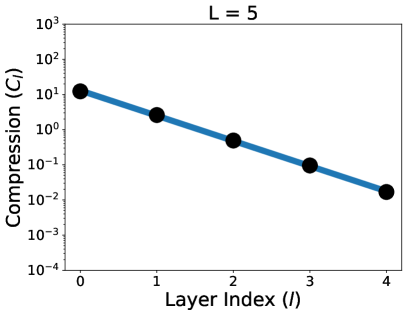
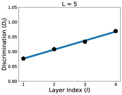
(a) 5-layer DLN with Kaiming Init.

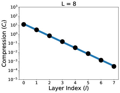
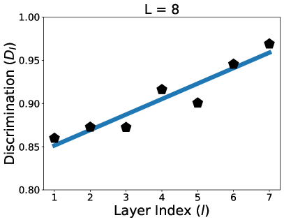
(b) 8-layer DLN with Kaiming Init.

Figure 11: Progressive feature compression and discrimination on DLNs with default PyTorch initialization. We train DLNs with uniform weight initialization and plot the dynamics of $C_{l}$ and $D_{l}$. We can observe progressive linear decay of $C_{l}$ still happens without the orthogonal initialization while the expanding pattern of $D_{l}$ disappears.

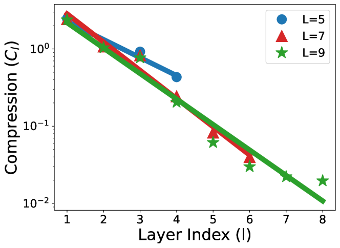
(a) FashionMNIST

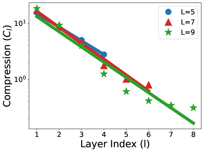
(b) CIFAR-10

Figure 12: Progressive feature compression on DLNs trained with default initialization and real datasets. Using the DLNs trained in Figure 3, we plot the within-class compression metrics $C_{l}$ against the layer indices. It is observed that progressive linear decay still (approximately) happens without the orthogonal initialization and datasets described in 1.

5.3.2 Implication on Transfer Learning

In this subsection, we experimentally substantiate our claims on transfer learning in Section 3 on practical nonlinear networks and real datasets, demonstrating that features before projection heads are less collapsed and exhibit better transferability. To support our argument, we conduct our experiments based on the following setup.

Network architectures.

We employ a ResNet18 backbone architecture [56], incorporating $t\in\{1,2,3,4,5\}$ layers of projection heads between the feature extractor and the final classifier, respectively. Here, one layer of the projection head consists of a linear layer followed by a ReLU activation layer. These projection layers are only used in the pre-training phase. On the downstream tasks, they are discarded, and a new linear classifier is trained on the downstream dataset.

Training datasets and training methods.

We use the CIFAR-100 and CIFAR-10 dataset in the pre-training and fine-tuning tasks, respectively. We train the networks using the Rescaled-MSE loss [46], with hyperparameters set to $k=5$ and $M=20$ for 200 epochs. During pre-training, we employed the SGD optimizer with a momentum of 0.9, a weight decay of $5\times 10^{-4}$, and a dynamically adaptive learning rate ranging from $10^{-2}$ to $10^{-5}$, modulated by a CosineAnnealing learning rate scheduler [72]. During the fine-tuning phase, we freeze all the parameters of the pre-trained model and only conduct linear probing. In other words, we only train a linear classifier on the downstream data for an additional 200 epochs. We run each experiment with 3 different random seeds.

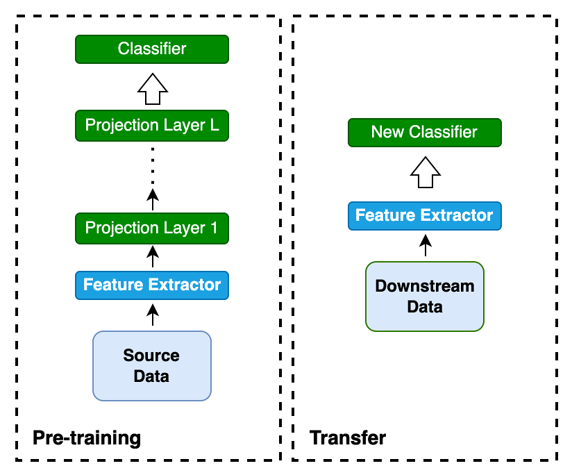
(a) Illustration on the usage of projection heads

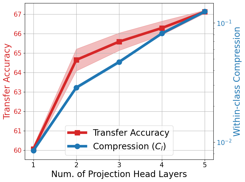
(b) Transfer learning results

Figure 13: Adding projection heads mitigates feature collapse and improves transfer accuracy. We pre-train ResNet18 backbones with 1 to 5 layers of projection heads on the CIFAR-100 dataset. After pre-training, we drop the projection heads and compute the metric $C_{l}$ on the learned features. Finally, we linearly probe the pre-trained models on the CIFAR-10 dataset and plot the evolution of $C_{l}$ alongside the corresponding transfer learning performance against the number of projection head layers. The shaded area represents the standard deviation of $3$ random seeds. The plot shows a clear trend that adding more layers of projection heads mitigates feature collapse and improves transfer learning results.

Experiments and observations.

Figure 13 illustrates the relationship between the number of layers in a projection head and two distinct metrics: (i) the compression metric $C_{l}$ of the learn features on the pre-trained dataset (depicted by the blue curve), and (ii) the transfer accuracy of pre-trained models on downstream tasks (depicted by the red curve). It is observed from Figure 13(b) that an increase in the number of layers in the projection head leads to decreased feature compression and better transfer accuracy.

These observations confirm our theoretical understanding that feature compression occurs progressively through the layers from shallow to deep and that the use of projection heads during the pre-training phase helps to prevent feature collapse at the feature extractor layer, thereby improving the model’s transfer accuracy on new downstream data. Furthermore, adding more layers in the projection head tends to preserve diverse features of the pre-trained model, resulting in improved transfer learning performance.

6 Conclusion

In this work, we studied hierarchical representations of deep networks by investigating intermediate features. In the context of training DLNs for solving multi-class classification problems, we explored the evolution of features across layers by analyzing within-class feature compression and between-class feature discrimination. We showed that under mild assumptions regarding the input data and trained weights, each layer of a DLN progressively compresses within-class features at a geometric rate and discriminates between-class features at a linear rate w.r.t. the layer index. Moreover, we discussed the implications of our results for deep learning practices related to interpretation, architecture design, and transfer learning. Our extensive experimental results on synthetic and real data sets not only support our theoretical findings but also illuminate our results regarding deep nonlinear networks.

Our work has opened many interesting directions to be further explored. First, our extensive experiments have demonstrated analogous patterns of progressive compression and discrimination phenomena in deep nonlinear networks. Extending our analysis to deep nonlinear networks emerges as a natural and promising direction for future research. Second, [114, 44] demonstrated that the outputs of self-attention layers in transformers exhibit a similar progressive compression phenomenon. It would be interesting to study this phenomenon in transformers based on our proposed framework.

Supplementary Material

Appendix A Auxiliary Results

Lemma 1.

Given a matrix $\bm{A}\in\mathbb{R}^{m\times n}$ of rank $r\in\mathbb{N}_{+}$, we have

$$\|\bm{A}^{T}\bm{A}\|_{F}\leq\|\bm{A}\|_{F}^{2}\leq\sqrt{r}\|\bm{A}^{T}\bm{A}\|_{F}.$$ (21)

Proof.

Let $\bm{A}=\bm{U}\bm{\Sigma}\bm{V}^{T}$ be a singular value decomposition of $\bm{A}$, where

$$\bm{\Sigma}=\begin{bmatrix}\tilde{\bm{\Sigma}}&\bm{0}\\ \bm{0}&\bm{0}\end{bmatrix},\ \tilde{\bm{\Sigma}}=\operatorname{diag}(\sigma_{1},\dots,\sigma_{r}),$$

$\bm{U}\in\mathcal{O}^{m}$, and $\bm{V}\in\mathcal{O}^{n}$. Then we compute

$$\|\bm{A}^{T}\bm{A}\|_{F}^{2}=\|\bm{\Sigma}^{T}\bm{\Sigma}\|_{F}^{2}=\sum_{i=1}^{r}\sigma_{i}^{4},\ \|\bm{A}\|_{F}^{2}=\|\bm{\Sigma}\|_{F}^{2}=\sum_{i=1}^{r}\sigma_{i}^{2},$$

which, together with the AM-QM inequality, directly implies (21). ∎

Lemma 2.

For arbitrary matrices $\bm{A},\bm{B}\in\mathbb{R}^{n\times n}$, if $\bm{A}$ has full column rank and $\bm{B}\neq\bm{0}$ or $\bm{B}$ has full row rank and $\bm{A}\neq\bm{0}$, it holds that

$$\sigma_{\min}\left(\bm{A}\bm{B}\right)\geq\sigma_{\min}\left(\bm{A}\right)\sigma_{\min}\left(\bm{B}\right).$$ (22)

Lemma 3.

Suppose that $\bm{Q}\in\mathcal{O}^{d\times K}$ is an orthonormal matrix and $\bm{A}\in\mathbb{R}^{K\times K}$ is a symmetric matrix of full rank, where $d>K$. Let $\bm{U}\bm{\Lambda}\bm{U}^{T}=\bm{Q}\bm{A}\bm{Q}^{T}$ be a compact singular value decomposition of $\bm{Q}\bm{A}\bm{Q}^{T}$, where $\bm{U}\in\mathcal{O}^{d\times K}$ and $\bm{\Lambda}\in\mathbb{R}^{K\times K}$ is a diagonal matrix. Then, it holds that

$$\bm{Q}\bm{Q}^{T}=\bm{U}\bm{U}^{T}.$$ (23)

Proof.

It follows from $\bm{U}\bm{\Lambda}\bm{U}^{T}=\bm{Q}\bm{A}\bm{Q}^{T}$, $\bm{Q}\in\mathcal{O}^{d\times K}$, and $\bm{U}\in\mathcal{O}^{d\times K}$ that

$$\bm{Q}^{T}\bm{U}\bm{\Lambda}=\bm{A}\bm{Q}^{T}\bm{U}.$$ (24)

Now, left-multiplying both sides by $\bm{Q}$ yields

$$\bm{Q}\bm{Q}^{T}\bm{U}\bm{\Lambda}=\bm{Q}\bm{A}\bm{Q}^{T}\bm{U}=\bm{U}\bm{\Lambda}\bm{U}^{T}\bm{U}=\bm{U}\bm{\Lambda}.$$

Since $\bm{A}$ is a symmetric matrix of full rank, $\bm{\Lambda}$ is a diagonal matrix with non-zero entries. We can multiply both sides by $\bm{\Lambda}^{-1}$ and obtain $\bm{Q}\bm{Q}^{T}\bm{U}=\bm{U}$, which implies (23) by $\bm{U}\in\mathcal{O}^{d\times K}$.

∎

Lemma 4.

For every real number $1\leq\theta\leq 1$ and $x\geq-1$, it holds that

$$(1+x)^{\theta}\leq 1+\theta x.$$

Appendix B Proofs of Main Results

In this section, we provide formal proofs to show our main result in 1 concerning the behavior of within-class and between-class features. This involves establishing some key properties of the weight matrices of each layer under Assumptions 1 and 2. The rest of this section is organized as follows: In Section B.1, we establish some preliminary results for weight matrices under Assumptions 1 and 2. In Section B.2, we prove that within-class features are compressed across layers at a geometric rate. In Section B.3, we prove that between-class features are discriminated across layers at a linear rate. Finally, we finish the proofs of 1 and 1 in Section B.4 and B.5, respectively.

Before we proceed, let us introduce some further notation that will be used throughout this section. Using (10), $\bm{Y}=\bm{I}_{K}\otimes\bm{1}_{n}^{\top}$, and Assumption 1, we show that the rank of $\bm{W}_{l}$ is at least $K$ for each $l\in[L]$; see Lemma 7. For all $l\in[L-1]$, let

$$\bm{W}_{l}=\bm{U}_{l}\bm{\Sigma}_{l}\bm{V}_{l}^{\top}=\begin{bmatrix}\bm{U}_{l,1}&\bm{U}_{l,2}\end{bmatrix}\begin{bmatrix}\bm{\Sigma}_{l,1}&\bm{0}\\ \bm{0}&\bm{\Sigma}_{l,2}\end{bmatrix}\begin{bmatrix}\bm{V}_{l,1}^{\top}\\ \bm{V}_{l,2}^{\top}\end{bmatrix}=\bm{U}_{l,1}\bm{\Sigma}_{l,1}\bm{V}_{l,1}^{\top}+\bm{U}_{l,2}\bm{\Sigma}_{l,2}\bm{V}_{l,2}^{\top},$$ (25)

be a singular value decomposition (SVD) of $\bm{W}_{l}$, where $\bm{\Sigma}_{l}\in\mathbb{R}^{d\times d}$ is diagonal, $\bm{\Sigma}_{l,1}=\operatorname{diag}\left(\sigma_{l,1},\dots,\sigma_{l,K}\right)$ with $\sigma_{l,1}\geq\cdots\geq\sigma_{l,K}>0$ being the first $K$ leading singular values of $\bm{W}_{l}$, and $\bm{\Sigma}_{l,2}=\operatorname{diag}\left(\sigma_{l,K+1},\dots,\sigma_{l,d}\right)$ with $\sigma_{l,K+1}\geq\cdots\geq\sigma_{l,d}\geq 0$ being the remaining singular values; $\bm{U}_{l}\in\mathcal{O}^{d}$ with $\bm{U}_{l,1}\in\mathbb{R}^{d\times K}$, $\bm{U}_{l,2}\in\mathbb{R}^{d\times(d-K)}$; $\bm{V}_{l}\in\mathcal{O}^{d}$ with $\bm{V}_{l,1}\in\mathbb{R}^{d\times K}$, $\bm{V}_{l,2}\in\mathbb{R}^{d\times(d-K)}$. Noting that $\bm{W}_{L}\in\mathbb{R}^{K\times d}$, let

$$\bm{W}_{L}=\bm{U}_{L}\bm{\Sigma}_{L}\bm{V}_{L}^{\top}=\bm{U}_{L}\begin{bmatrix}\bm{\Sigma}_{L,1}&\bm{0}\end{bmatrix}\begin{bmatrix}\bm{V}_{L,1}^{\top}\\ \bm{V}_{L,2}^{\top}\end{bmatrix}=\bm{U}_{L}\bm{\Sigma}_{L,1}\bm{V}_{L,1}^{\top},$$ (26)

be an SVD of $\bm{W}_{L}$, where $\bm{\Sigma}_{L}\in\mathbb{R}^{K\times d}$, and $\bm{\Sigma}_{L,1}=\operatorname{diag}\left(\sigma_{L,1},\dots,\sigma_{L,K}\right)$ with $\sigma_{L,1}\geq\cdots\geq\sigma_{L,K}>0$ being the singular values; $\bm{U}_{L}\in\mathcal{O}^{K}$, and $\bm{V}_{L}\in\mathcal{O}^{d}$ with $\bm{V}_{L,1}\in\mathbb{R}^{d\times K}$, $\bm{V}_{L,2}\in\mathbb{R}^{d\times(d-K)}$. Moreover, we respectively denote the $k$-th class mean and global mean by

$$\bar{\bm{x}}_{k}=\frac{1}{n}\sum_{i=1}^{N}\bm{x}_{k,i},\quad\bar{\bm{x}}=\frac{1}{K}\sum_{k=1}^{K}\bar{\bm{x}}_{k},$$ (27)

and let

$$\bar{\bm{X}}=\left[\bar{\bm{x}}_{1}\ \bar{\bm{x}}_{2}\ \dots\ \bar{\bm{x}}_{K}\right]\otimes\bm{1}_{n}^{\top}\in\mathbb{R}^{d\times N}.$$ (28)

Note that we shall use the above notation repeatedly in the following context.

B.1 Properties of Weight Matrices

In this subsection, we establish some properties of weight matrices $\{\bm{W}_{l}\}_{l=1}^{L}$ under Assumptions 1 and 2. Towards this goal, we first prove some inequalities on the spectrum of the data matrix $\bm{X}$ and the distance between $\bm{X}$ and $\bar{\bm{X}}$ under Assumption 1. These inequalities will serve as crucial components in the subsequent analysis of the spectral properties of the weight matrices.

Lemma 5.

Suppose that Assumption 1 holds. Then, we have

$$\sqrt{1-\theta}\leq\sigma_{\min}(\bm{X})\leq\sigma_{\max}(\bm{X})\leq\sqrt{1+\theta},$$ (29)

$$\|\bm{X}-\bar{\bm{X}}\|\leq\sqrt{1+4\theta},\quad N-K-4\theta\leq\|\bm{X}-\bar{\bm{X}}\|_{F}^{2}\leq N-K+4\theta.$$ (30)

Proof.

Using $\|\bm{A}\|\leq\|\bm{A}\|_{F}$ for all $\bm{A}\in\mathbb{R}^{N\times N}$, we have

$$\|\bm{X}^{\top}\bm{X}-\bm{I}_{N}\|^{2}\leq\|\bm{X}^{\top}\bm{X}-\bm{I}_{N}\|_{F}^{2}\leq\sum_{i=1}^{N}\left(\|\bm{x}_{i}\|^{2}-1\right)^{2}+\sum_{i=1}^{N}\sum_{j\neq i}^{N}\left(\bm{x}_{i}^{\top}\bm{x}_{j}\right)^{2}\leq\theta^{2},$$ (31)

where the last inequality follows from (9). This, together with Weyl’s inequality, implies $1-\theta\leq\sigma_{\min}(\bm{X}^{\top}\bm{X})\leq\sigma_{\max}(\bm{X}^{\top}\bm{X})\leq 1+\theta$. Therefore, we obtain (29).

Now, we prove (30). For ease of exposition, let $\bm{A}:=(\bm{X}-\bar{\bm{X}})^{\top}(\bm{X}-\bar{\bm{X}})=\bm{X}^{\top}\bm{X}-\bm{X}^{\top}\bar{\bm{X}}-\bar{\bm{X}}^{\top}\bm{X}+\bar{\bm{X}}^{\top}\bar{\bm{X}}$. First, we consider the elements of diagonal blocks of $\bm{A}$. For each $i=(k-1)n+j$ and $j\in[n]$, we compute

$$a_{ii} =\left\|\bm{x}_{k,j}-\bar{\bm{x}}_{k}\right\|^{2}=\left(1-\frac{1}{n}\right)^{2}\|\bm{x}_{k,j}\|^{2}+\frac{1}{n^{2}}\sum_{j^{\prime}\neq j}\|\bm{x}_{k,j^{\prime}}\|^{2}-$$

$$\quad\frac{2}{n}\sum_{j\neq j^{\prime}}\langle\bm{x}_{k,j},\bm{x}_{k,j^{\prime}}\rangle+\frac{1}{n^{2}}\sum_{j=1}^{n}\sum_{j^{\prime}\neq j}\langle\bm{x}_{k,j},\bm{x}_{k,j^{\prime}}\rangle.$$

This, together with (9) in Assumption 1, yields

$$1-\frac{1}{n}-\frac{4\theta}{N}\leq a_{ii}\leq 1-\frac{1}{n}+\frac{4\theta}{N}.$$ (32)

Using the similar argument, we compute for each $i=(k-1)n+j$, $i^{\prime}=(k-1)n+j^{\prime}$, and $j\neq j^{\prime}\in[n]$,

$$-\frac{1}{n}-\frac{4\theta}{N}\leq a_{i,i^{\prime}}\leq-\frac{1}{n}+\frac{4\theta}{N}.$$ (33)

Now, we consider the elements of off-diagonal blocks of $\bm{A}$. Similarly, we compute for each $i=(k-1)n+j$, $i^{\prime}=(k^{\prime}-1)n+j^{\prime}$, $k\neq k^{\prime}$, and $j,j^{\prime}\in[n]$,

$$-\frac{4\theta}{N}\leq a_{i,i^{\prime}}\leq\frac{4\theta}{N}.$$ (34)

This, together with (32) and (33), yields that

$$\bm{A}=\bm{I}_{N}-\frac{1}{n}I_{K}\otimes\bm{E}_{n}+\bm{\Delta},$$ (35)

where $|\delta_{ij}|\leq{4\theta}/{N}$. Therefore, we have

$$\|\bm{A}\|\leq\left\|\bm{I}_{N}-\frac{1}{n}I_{K}\otimes\bm{E}_{n}\right\|+\|\bm{\Delta}\|_{F}\leq 1+4\theta,$$

which implies the first inequality in (30).

Moreover, we have

$$\|\bm{X}-\bar{\bm{X}}\|_{F}^{2}=\|\bm{X}\|_{F}^{2}-2\langle\bm{X},\bar{\bm{X}}\rangle+\|\bar{\bm{X}}\|_{F}^{2}.$$ (36)

Then, we will bound the above terms in turn. First, noting that $\|\bm{X}\|_{F}^{2}=\sum_{i=1}^{N}\|\bm{x}_{i}\|^{2}$ and using (9) in Assumption 1 yield

$$N-\theta\leq\|\bm{X}\|_{F}^{2}\leq N+\theta.$$ (37)

Second, it follows from (27) that

$$\langle\bm{X},\bar{\bm{X}}\rangle=\sum_{k=1}^{K}\sum_{i=1}^{n}\langle\bm{x}_{k,i},\bar{\bm{x}}_{k}\rangle=\sum_{k=1}^{K}\sum_{i=1}^{n}\frac{1}{n}\sum_{j=1}^{n}\langle\bm{x}_{k,i},\bm{x}_{k,j}\rangle=\sum_{k=1}^{K}\sum_{i=1}^{n}\frac{1}{n}\left(\|\bm{x}_{k,i}\|^{2}+\sum_{j\neq i}^{n}\langle\bm{x}_{k,i},\bm{x}_{k,j}\rangle\right).$$

This, together with Assumption 1, yields

$$K-\theta\leq\langle\bm{X},\bar{\bm{X}}\rangle\leq K+\theta.$$ (38)

Finally, we compute

$$\|\bar{\bm{X}}\|_{F}^{2}=n\sum_{k=1}^{K}\|\bar{\bm{x}}_{k}\|^{2}=\frac{1}{n}\sum_{k=1}^{K}\left\|\sum_{i=1}^{n}\bm{x}_{k,i}\right\|^{2}=\frac{1}{n}\sum_{k=1}^{K}\left(\sum_{i=1}^{n}\|\bm{x}_{k,i}\|^{2}+\sum_{i\neq j}\langle\bm{x}_{k,i},\bm{x}_{k,j}\rangle\right)$$

This, together with Assumption 1, yields

$$K-\theta\leq\|\bar{\bm{X}}\|_{F}^{2}\leq K+\theta.$$ (39)

Substituting (37), (38), and (39) into (36) yields the second inequality in (30). ∎

Next, we present a lemma that shows that each singular value of the first $L-1$ weight matrices is exactly the same, and each singular value of the last weight matrix is approximately equal to that of the first $L-1$ weight matrices under the balancedness (11) in Assumption 2.

Lemma 6.

Suppose that the weight matrices $\{\bm{W}_{l}\}_{l=1}^{L}$ satisfy (11) and admit the SVD in (25) and (26). Then, it holds that

$$\bm{\Sigma}_{l+1}=\bm{\Sigma}_{l},\ \forall l\in[L-2],\ \|\bm{\Sigma}_{L}^{\top}\bm{\Sigma}_{L}-\bm{\Sigma}_{l}^{2}\|_{F}\leq\delta,\ \forall l\in[L-1].$$ (40)

Proof.

Since $\bm{W}_{l+1}^{\top}\bm{W}_{l+1}=\bm{W}_{l}\bm{W}_{l}^{\top}$ for all $l\in[L-2]$ and (25), we have

$$\bm{V}_{l+1}\bm{\Sigma}_{l+1}^{2}\bm{V}_{l+1}^{\top}=\bm{U}_{l}\bm{\Sigma}_{l}^{2}\bm{U}_{l}^{\top}.$$ (41)

For a given $l\in[L-2]$, the two sides of the above equation are essentially eigenvalue decomposition of the same matrix. This, together with the fact that $\bm{\Sigma}_{l+1}$ and $\bm{\Sigma}_{l}$ have non-increasing and non-negative diagonal elements by (25), yields $\bm{\Sigma}_{l+1}=\bm{\Sigma}_{l}$. Using $\|\bm{W}_{L}^{\top}\bm{W}_{L}-\bm{W}_{L-1}\bm{W}_{L-1}^{\top}\|_{F}\leq\delta$, (25), and (26), we have

$$\|\bm{V}_{L}\bm{\Sigma}_{L}^{\top}\bm{\Sigma}_{L}\bm{V}_{L}^{\top}-\bm{U}_{L-1}\bm{\Sigma}_{L-1}^{2}\bm{U}_{L-1}^{\top}\|_{F}\leq\delta.$$ (42)

This, together with [2, Lemma 4], implies $\|\bm{\Sigma}_{L}^{\top}\bm{\Sigma}_{L}-\bm{\Sigma}_{L-1}^{2}\|_{F}\leq\delta$. According to this and $\bm{\Sigma}_{l+1}=\bm{\Sigma}_{l}$ for all $l\in[L-2]$, implies (40) for all $l\in[L-1]$. ∎

Based on the above two lemmas, we are ready to estimate the top $K$ singular values of each weight matrix $\bm{W}_{l}$ for all $l\in[L]$ under Assumptions 1 and 2.

Lemma 7.

Suppose that Assumption 1 holds, and the weight matrices $\{\bm{W}_{l}\}_{l=1}^{L}$ satisfy (10) and (11) with

$$\delta\leq\frac{(2n)^{1/L}}{30L^{2}}.$$ (43)

Then, the following statements hold:
(i) It holds that

$$\frac{\sqrt{n}}{\sqrt{1+\theta}}\leq\sigma_{K}(\bm{W}_{L:1})\leq\sigma_{1}(\bm{W}_{L:1})\leq\frac{\sqrt{n}}{\sqrt{1-\theta}},$$ (44)

(ii) It holds that

$$\left(\sqrt{\frac{n}{2}}\right)^{1/L}\leq\sigma_{K}\left(\bm{W}_{l}\right)\leq\sigma_{1}\left(\bm{W}_{l}\right)\leq\left(2\sqrt{n}\right)^{1/L},\ \forall l\in[L],$$ (45)

and

$$\left(\left(\frac{1}{1+\theta}-4\delta\right)n\right)^{1/2L}\leq\sigma_{K}(\bm{W}_{l})\leq\sigma_{1}(\bm{W}_{l})\leq\left(\left(\frac{1}{1-\theta}+4\delta\right)n\right)^{1/2L},\ \forall l\in[L-1],$$ (46)

$$\left(\left(\frac{1}{1+\theta}-4\delta\right)n\right)^{1/2L}-\sqrt{\delta}\leq\sigma_{K}(\bm{W}_{L})\leq\sigma_{1}(\bm{W}_{L})\leq\left(\left(\frac{1}{1-\theta}+4\delta\right)n\right)^{1/2L}+\sqrt{\delta}.$$ (47)

Proof.

According to (29) in Lemma 5, we obtain that $\bm{X}$ is of full column rank, and thus $\bm{X}^{+}:=(\bm{X}^{\top}\bm{X})^{-1}\bm{X}^{\top}$ is of full row rank with

$$1/\sqrt{1+\theta}\leq\sigma_{\min}(\bm{X}^{+})\leq\sigma_{\max}(\bm{X}^{+})\leq 1/\sqrt{1-\theta}.$$ (48)

This, together with $\bm{Y}=\bm{I}_{K}\otimes\bm{1}_{n}^{\top}$, (10), and Lemma 2, yields that

$$\frac{\sqrt{n}}{\sqrt{1+\theta}}\leq\sigma_{K}(\bm{W}_{L:1})\leq\sigma_{1}(\bm{W}_{L:1})\leq\frac{\sqrt{n}}{\sqrt{1-\theta}},$$ (49)

which, together with $\theta\in[0,1/4]$, implies

$$\frac{2\sqrt{n}}{\sqrt{5}}\leq\sigma_{K}(\bm{W}_{L:1})\leq\sigma_{1}(\bm{W}_{L:1})\leq\frac{2\sqrt{n}}{\sqrt{3}}.$$ (50)

Using this, (11) with (43), and invoking [2, Lemma 6], we obtain $\sigma_{1}(\bm{W}_{l})\leq\left(2\sqrt{n}\right)^{1/L}$ for all $l\in[L]$. Using $\bm{W}_{l+1}^{\top}\bm{W}_{l+1}=\bm{W}_{l}\bm{W}_{l}^{\top}$ for all $l\in[L-2]$ by (11), we compute

$$\|\bm{W}_{L:1}^{\top}\bm{W}_{L:1}-\left(\bm{W}_{1}^{\top}\bm{W}_{1}\right)^{L}\|_{F} =\|\bm{W}_{L:1}^{\top}\bm{W}_{L:1}-\bm{W}_{L-1:1}^{\top}\bm{W}_{L-1}\bm{W}_{L-1}^{\top}\bm{W}_{L-1:1}\|_{F}$$

$$=\|\bm{W}_{L-1:1}^{\top}\left(\bm{W}_{L}^{\top}\bm{W}_{L}-\bm{W}_{L-1}\bm{W}_{L-1}^{\top}\right)\bm{W}_{L-1:1}\|_{F}$$

$$\leq\|\bm{W}_{L}^{\top}\bm{W}_{L}-\bm{W}_{L-1}\bm{W}_{L-1}^{\top}\|_{F}\prod_{l=1}^{L-1}\|\bm{W}_{l}\|^{2}$$

$$\leq\delta\left(4n\right)^{(L-1)/L}\leq\frac{2n}{15L^{2}},$$ (51)

where the second inequality uses (11), (43), and (45) for all $l\in[L-1]$, and the last inequality follows from (43). Using this, (49), and Weyl’s inequality gives

$$\sigma_{K}\left(\left(\bm{W}_{1}^{\top}\bm{W}_{1}\right)^{L}\right) \geq\sigma_{K}\left(\bm{W}_{L:1}^{\top}\bm{W}_{L:1}\right)-\|\bm{W}_{L:1}^{\top}\bm{W}_{L:1}-\left(\bm{W}_{1}^{\top}\bm{W}_{1}\right)^{L}\|$$

$$\geq\frac{n}{1+\theta}-\|\bm{W}_{L:1}^{\top}\bm{W}_{L:1}-\left(\bm{W}_{1}^{\top}\bm{W}_{1}\right)^{L}\|_{F}\geq\left(\frac{1}{1+\theta}-\frac{2}{15L^{2}}\right)n,$$

which implies $\sigma_{K}(\bm{W}_{1})\geq\left(\left(\frac{1}{1+\theta}-\frac{2}{15L^{2}}\right)n\right)^{1/2L}$. This, together with Lemma 6, further implies

$$\sigma_{K}(\bm{W}_{l})\geq\left(\left(\frac{1}{1+\theta}-\frac{2}{15L^{2}}\right)n\right)^{1/2L},\ \forall l\in[L-1].$$ (52)

Using Weyl’s inequality again and (11), we have

$$\sigma_{K}\left(\bm{W}_{L}^{\top}\bm{W}_{L}\right) \geq\sigma_{K}\left(\bm{W}_{L-1}^{\top}\bm{W}_{L-1}\right)-\|\bm{W}_{L}^{\top}\bm{W}_{L}-\bm{W}_{L-1}\bm{W}_{L-1}^{\top}\|$$

$$\geq\left(\frac{1}{1+\theta}-\frac{2}{15L^{2}}\right)^{1/L}n^{1/L}-\delta\geq\left(\frac{n}{2}\right)^{1/L},$$

where the last inequality follows from $\delta\leq(2n)^{1/L}/(30L^{2})$ and

$$\left(\frac{1}{1+\theta}-\frac{2}{15L^{2}}\right)^{1/L}\geq\left(\frac{3}{4}\right)^{1/L}\geq\frac{1}{15L^{2}}+\left(\frac{1}{2}\right)^{1/L},\ \forall L\geq 1.$$

Here the first inequality uses $L\geq 2$, and the second inequality is due to $f(x)=(3/4)^{x}-(1/2)^{x}-x^{2}/15$ is increasing for $x\in(0,1]$ and $f(0)=0$. Therefore, we have $\sigma_{K}(\bm{W}_{L})\geq\left(\frac{n}{2}\right)^{1/2L}$. This, together with (52) and $\sigma_{1}(\bm{W}_{l})\leq\left(2\sqrt{n}\right)^{1/L}$ for all $l\in[L]$, yields (45).

Next, we are devoted to proving (46) and (47). It follows from (B.1) that

$$\|\bm{W}_{L:1}^{\top}\bm{W}_{L:1}-\left(\bm{W}_{1}^{\top}\bm{W}_{1}\right)^{L}\|_{F}\leq 4n\delta.$$ (53)

This, together with Weyl’s inequality and (49), yields

$$\sigma_{1}\left(\left(\bm{W}_{1}^{\top}\bm{W}_{1}\right)^{L}\right) \leq\sigma_{1}\left(\bm{W}_{L:1}^{\top}\bm{W}_{L:1}\right)+\|\bm{W}_{L:1}^{\top}\bm{W}_{L:1}-\left(\bm{W}_{1}^{\top}\bm{W}_{1}\right)^{L}\|\leq\left(\frac{1}{1-\theta}+4\delta\right)n,$$

$$\sigma_{K}\left(\left(\bm{W}_{1}^{\top}\bm{W}_{1}\right)^{L}\right) \geq\sigma_{K}\left(\bm{W}_{L:1}^{\top}\bm{W}_{L:1}\right)-\|\bm{W}_{L:1}^{\top}\bm{W}_{L:1}-\left(\bm{W}_{1}^{\top}\bm{W}_{1}\right)^{L}\|\geq\left(\frac{1}{1+\theta}-4\delta\right)n.$$

This, together with Lemma 6, directly implies (46). Using Weyl’s inequality and (11), we have

$$\sigma_{1}\left(\bm{W}_{L}^{\top}\bm{W}_{L}\right) \leq\sigma_{1}\left(\bm{W}_{L-1}^{\top}\bm{W}_{L-1}\right)+\|\bm{W}_{L}^{\top}\bm{W}_{L}-\bm{W}_{L-1}\bm{W}_{L-1}^{\top}\|\leq\left(\frac{1}{1-\theta}+4\delta\right)^{1/L}n^{1/L}+\delta,$$

$$\sigma_{K}\left(\bm{W}_{L}^{\top}\bm{W}_{L}\right) \geq\sigma_{K}\left(\bm{W}_{L-1}^{\top}\bm{W}_{L-1}\right)-\|\bm{W}_{L}^{\top}\bm{W}_{L}-\bm{W}_{L-1}\bm{W}_{L-1}^{\top}\|\geq\left(\frac{1}{1-\theta}+4\delta\right)^{1/L}n^{1/L}-\delta,$$

which directly implies (47). ∎

Using this lemma and $\varepsilon\in(0,1)$, we conclude that the leading $K$ singular values of $\bm{W}_{l}$ for all $l\in[L-1]$ are well separated from the remaining $d-K$ singular values according to (12). Consequently, we can handle them with the associated singular vectors separately. Since $\bm{\Sigma}_{l+1}=\bm{\Sigma}_{l}$ for all $l\in[L-2]$ according to Lemma 6, suppose that $\bm{\Sigma}_{l,1}$ and $\bm{\Sigma}_{l,2}$ have distinct $p\geq 1$ and $q\geq 1$ singular values for all $l\in[L-1]$, respectively. Let $\sigma_{1}>\dots>\sigma_{p}>\sigma_{p+1}>\dots>\sigma_{p+q}$ be the distinct singular values with the corresponding multiplicities $h_{1},h_{2},\dots,h_{p+q}\in\mathbb{N}$. In particular, we have $\sum_{i=1}^{p}h_{i}=K$, $\sum_{i=p+1}^{p+q}h_{i}=d-K$, and $\sigma_{p+1}\leq\varepsilon$ due to (12). Then, we can write

$$\bm{\Sigma}_{l}=\tilde{\bm{\Sigma}}={\rm BlkDiag}(\tilde{\bm{\Sigma}}_{1},\tilde{\bm{\Sigma}}_{2})={\rm BlkDiag}\left(\sigma_{1}\bm{I}_{h_{1}},\dots,\sigma_{p}\bm{I}_{h_{p}},\dots,\sigma_{p+q}\bm{I}_{h_{p+q}}\right).$$ (54)

Using the same partition, we can also write

$$\bm{U}_{l}=\left[\bm{U}_{l}^{(1)},\dots,\bm{U}_{l}^{(p)},\dots,\bm{U}_{l}^{(p+q)}\right],\ \bm{V}_{l}=\left[\bm{V}_{l}^{(1)},\dots,\bm{V}_{l}^{(p)},\dots,\bm{V}_{l}^{(p+q)}\right],$$ (55)

where $\bm{U}_{l}^{(i)},\bm{V}_{l}^{(i)}\in\mathcal{O}^{d\times h_{i}}$ for all $i\in[p+q]$. Using the above definitions, we can characterize the relationship between singular vector matrices $\bm{U}_{l}$ and $\bm{V}_{l+1}$.

Lemma 8.

Suppose that Assumptions 1 and 2 hold. Then, the following statements hold:
(i) For all $l\in[L-2]$, there exists orthogonal matrix $\bm{Q}_{l,i}\in\mathcal{O}^{h_{i}}$ such that

$$\bm{U}_{l}^{(i)}=\bm{V}_{l+1}^{(i)}\bm{Q}_{l,i},\ \forall i\in[p+q].$$ (56)

(ii) It holds that

$$\|\bm{V}_{L,1}^{\top}\bm{U}_{L-1,2}\|_{F}\leq\frac{2\sqrt{\delta}\sqrt[4]{K}}{n^{1/2L}},\ \sigma_{\min}\left(\bm{V}_{L,1}^{\top}\bm{U}_{L-1,1}\right)\geq 1-\frac{2\sqrt{\delta}\sqrt[4]{K}}{n^{1/2L}}.$$ (57)

Proof.

(i) Using the first equation in (40), (41), (54), and (55), we obtain

$$\sum_{i=1}^{p+q}\sigma_{i}^{2}\bm{V}_{l+1}^{(i)}\bm{V}_{l+1}^{(i)^{\top}}=\sum_{i=1}^{p+q}\sigma_{i}^{2}\bm{U}_{l}^{(i)}\bm{U}_{l}^{(i)^{\top}}$$

Multiplying $\bm{U}_{l}^{(1)}$ on the both sides of the above equality, we obtain

$$\sum_{i=1}^{p+q}\sigma_{i}^{2}\bm{U}_{l}^{(1)^{\top}}\bm{V}_{l+1}^{(i)}\bm{V}_{l+1}^{(i)^{\top}}\bm{U}_{l}^{(1)}=\sigma_{1}^{2}\bm{I},$$

where the equality follows from the fact that $\bm{U}_{l}\in\mathcal{O}^{d}$ takes the form of (55). Therefore, for any $\bm{x}\in\mathbb{R}^{h_{1}}$ with $\|\bm{x}\|=1$, we have

$$\sigma_{1}^{2} =\sum_{i=1}^{p+q}\sigma_{i}^{2}\left\|\bm{V}_{l+1}^{(i)^{\top}}\bm{U}_{l}^{(1)}\bm{x}\right\|^{2}\leq\sigma_{1}^{2}\left\|\bm{V}_{l+1}^{(1)^{\top}}\bm{U}_{l}^{(1)}\bm{x}\right\|^{2}+\sigma_{2}^{2}\sum_{i=2}^{p+q}\left\|\bm{V}_{l+1}^{(i)^{\top}}\bm{U}_{l}^{(1)}\bm{x}\right\|^{2}$$

$$=\sigma_{1}^{2}\left\|\bm{V}_{l+1}^{(1)^{\top}}\bm{U}_{l}^{(1)}\bm{x}\right\|^{2}+\sigma_{2}^{2}\left(1-\left\|\bm{V}_{l+1}^{(1)^{\top}}\bm{U}_{l}^{(1)}\bm{x}\right\|^{2}\right)=\sigma_{2}^{2}+\left(\sigma_{1}^{2}-\sigma_{2}^{2}\right)\left\|\bm{V}_{l+1}^{(1)^{\top}}\bm{U}_{l}^{(1)}\bm{x}\right\|^{2},$$

where the inequality follows from $\sigma_{1}>\sigma_{2}>\dots>\sigma_{p+q}$, and the second equality uses $\bm{V}_{l+1}\in\mathcal{O}^{d}$. This, together with $\sigma_{1}>\sigma_{2}>0$, implies $\left\|\bm{V}_{l+1}^{(1)^{\top}}\bm{U}_{l}^{(1)}\bm{x}\right\|^{2}=1$. Using this and $\|\bm{x}\|=1$, we have $\bm{U}_{l}^{(1)}=\bm{V}_{l+1}^{(1)}\bm{Q}_{l,1}$ for some $\bm{Q}_{l,1}\in\mathcal{O}^{h_{1}}$. By repeatedly applying the same argument to $\bm{U}_{l}^{(i)}$ for all $i\geq 2$, we prove (56).

(ii) According to (40) and the block structures of $\bm{\Sigma}_{L},\bm{\Sigma}_{L-1}$, we obtain

$$\|\bm{\Sigma}_{L-1,2}^{2}\|_{F}\leq\delta.$$ (58)

In addition, it follows from (25), (26), and (42) that

$$\|\bm{V}_{L,1}\bm{\Sigma}^{2}_{L,1}\bm{V}_{L,1}^{\top}-\bm{U}_{L-1,1}\bm{\Sigma}^{2}_{L-1,1}\bm{U}_{L-1,1}^{\top}-\bm{U}_{L-1,2}\bm{\Sigma}_{L-1,2}^{2}\bm{U}_{L-1,2}^{\top}\|_{F}\leq\delta.$$

Using this, $\|\bm{U}^{\top}\bm{A}\bm{U}\|_{F}\leq\|\bm{A}\|_{F}$ for any $\bm{U}\in\mathcal{O}^{d\times(d-K)}$, we further obtain

$$\|\bm{U}_{L-1,2}^{\top}\bm{V}_{L,1}\bm{\Sigma}^{2}_{L,1}\bm{V}_{L,1}^{\top}\bm{U}_{L-1,2}-\bm{\Sigma}_{L-1,2}^{2}\|_{F}\leq\delta.$$

This, together with (58), implies

$$\|\bm{U}_{L-1,2}^{\top}\bm{V}_{L,1}\bm{\Sigma}^{2}_{L,1}\bm{V}_{L,1}^{\top}\bm{U}_{L-1,2}\|_{F}\leq 2\delta.$$

Using Lemma 1 with the fact that $\bm{\Sigma}_{L,1}\bm{V}_{L,1}^{\top}\bm{U}_{L-1,2}$ is of rank $K$, we further have

$$\|\bm{\Sigma}_{L,1}\bm{V}_{L,1}^{\top}\bm{U}_{L-1,2}\|_{F}^{2}\leq 2\delta\sqrt{K}.$$ (59)

Noting that $\|\bm{\Sigma}_{L,1}\bm{V}_{L,1}^{\top}\bm{U}_{L-1,2}\|_{F}\geq\sigma_{\min}(\bm{\Sigma}_{L,1})\|\bm{V}_{L,1}^{\top}\bm{U}_{L-1,2}\|_{F}$, we have

$$\|\bm{V}_{L,1}^{\top}\bm{U}_{L-1,2}\|_{F}\leq\frac{\|\bm{\Sigma}_{L,1}\bm{V}_{L,1}^{\top}\bm{U}_{L-1,2}\|_{F}}{\sigma_{\min}(\bm{\Sigma}_{L,1})}\leq\frac{\sqrt{2\delta}\sqrt[4]{K}}{\left(n/2\right)^{1/2L}}\leq\frac{2\sqrt{\delta}\sqrt[4]{K}}{n^{1/2L}},$$ (60)

where the second inequality follows from (59) and Lemma 7. Now, we compute

$$\sigma_{\min}^{2}(\bm{V}_{L,1}^{\top}\bm{U}_{L-1,1}) =\min_{\|\bm{x}\|=1}\|\bm{U}_{L-1,1}^{\top}\bm{V}_{L,1}\bm{x}\|^{2}=\min_{\|\bm{x}\|=1}\bm{x}^{\top}\bm{V}_{L,1}^{\top}\bm{U}_{L-1,1}\bm{U}_{L-1,1}^{\top}\bm{V}_{L,1}\bm{x}$$

$$=\min_{\|\bm{x}\|=1}\bm{x}^{\top}\bm{V}_{L,1}^{\top}\left(\bm{I}-\bm{U}_{L-1,2}\bm{U}_{L-1,2}^{\top}\right)\bm{V}_{L,1}\bm{x}=1-\max_{\|\bm{x}\|=1}\|\bm{U}_{L-1,2}^{\top}\bm{V}_{L,1}\bm{x}\|^{2}$$

$$=1-\sigma_{\max}^{2}(\bm{U}_{L-1,2}^{\top}\bm{V}_{L,1})\geq 1-\|\bm{U}_{L-1,2}^{\top}\bm{V}_{L,1}\|_{F}^{2},$$

where the third equality follows from $\bm{U}_{L-1}\in\mathcal{O}^{d}$. This, together with (60), implies

$$\sigma_{\min}(\bm{V}_{L,1}^{\top}\bm{U}_{L-1,1})\geq\sqrt{1-\|\bm{U}_{L-1,2}^{\top}\bm{V}_{L,1}\|_{F}^{2}}\geq 1-\|\bm{U}_{L-1,2}^{\top}\bm{V}_{L,1}\|_{F}\geq 1-\frac{2\sqrt{\delta}\sqrt[4]{K}}{n^{1/2L}}.$$

∎

B.2 Analysis of Progressive Within-Class Compression

In this subsection, our goal is to prove progressive compression of within-class features across layers. Towards this goal, we study the behavior of $\mathrm{Tr}(\bm{\Sigma}_{W})$ and $\mathrm{Tr}(\bm{\Sigma}_{B})$ across layers, respectively. For ease of exposition, let

$$\bm{\Delta}_{W}:=\left[\bm{\delta}_{1,1},\dots,\bm{\delta}_{1,n},\dots,\bm{\delta}_{K,1},\dots,\bm{\delta}_{K,n}\right]\in\mathbb{R}^{d\times N},\ \text{where}\ \bm{\delta}_{k,i}=\bm{x}_{k,i}-\bar{\bm{x}}_{k},\ \forall k,i,$$ (61)

$$\bm{\Delta}_{B}:=\left[\bar{\bm{\delta}}_{1},\dots,\bar{\bm{\delta}}_{K}\right]\in\mathbb{R}^{d\times K},\ \text{where}\ \bar{\bm{\delta}}_{k}=\bar{\bm{x}}_{k}-\bar{\bm{x}},\ \forall k\in[K],$$ (62)

where $\bar{\bm{x}}_{k}$ and $\bar{\bm{x}}$ are defined in (27). According to Definition 1 and $n_{k}=n$ for all $k\in[K]$, one can verify

$$\mathrm{Tr}(\bm{\Sigma}_{W}^{l})=\frac{1}{N}\|\bm{W}_{l:1}\bm{\Delta}_{W}\|_{F}^{2},\quad\mathrm{Tr}(\bm{\Sigma}_{B}^{l})=\frac{1}{K}\|\bm{W}_{l:1}\bm{\Delta}_{B}\|_{F}^{2}.$$ (63)

Recall from (54) that $\tilde{\bm{\Sigma}}={\rm BlkDiag}(\tilde{\bm{\Sigma}}_{1},\tilde{\bm{\Sigma}}_{2})$, where

$$\tilde{\bm{\Sigma}}_{1}={\rm BlkDiag}\left(\sigma_{1}\bm{I}_{h_{1}},\dots,\sigma_{p}\bm{I}_{h_{p}}\right),\ \tilde{\bm{\Sigma}}_{2}={\rm BlkDiag}\left(\sigma_{p+1}\bm{I}_{h_{p+1}},\dots,\sigma_{p+q}\bm{I}_{h_{p+q}}\right)$$ (64)

According to (25), (54), and (56), there exist block diagonal matrices $\bm{O}_{l,1}=\mathrm{Blkdiag}(\bm{Q}_{l,1},\dots,\bm{Q}_{l,p})\in\mathbb{R}^{K\times K}$ and $\bm{O}_{l,2}=\mathrm{Blkdiag}(\bm{Q}_{l,p+1},\dots,\bm{Q}_{l,p+q})\in\mathbb{R}^{(d-K)\times(d-K)}$ with $\bm{Q}_{l,i}\in\mathcal{O}^{h_{i}}$ for all $i\in[p+q]$ such that for each $l\in[L-1]$,

$$\bm{W}_{l:1}=\bm{U}_{l,1}\bm{O}_{l,1}\tilde{\bm{\Sigma}}^{l}_{1}\bm{V}_{1,1}^{\top}+\bm{U}_{l,2}\bm{O}_{l,2}\tilde{\bm{\Sigma}}^{l}_{2}\bm{V}_{1,2}^{\top}=\bm{U}_{l,1}\tilde{\bm{\Sigma}}^{l}_{1}\bm{O}_{l,1}\bm{V}_{1,1}^{\top}+\bm{U}_{l,2}\tilde{\bm{\Sigma}}^{l}_{2}\bm{O}_{l,2}\bm{V}_{1,2}^{\top},$$ (65)

where $\bm{U}_{l,1}$, $\bm{U}_{l,2}$, $\bm{V}_{l,1}$, and $\bm{V}_{l,2}$ for ell $l\in[L-1]$ are defined in (25).

To bound $\mathrm{Tr}(\bm{\Sigma}_{W}^{l})$ and $\mathrm{Tr}(\bm{\Sigma}_{B}^{l})$ across layers, we present a lemma that establishes a relationship between the magnitudes of $\bm{V}_{1,1}^{\top}\bm{\Delta}_{W}$ and $\bm{V}_{1,2}^{\top}\bm{\Delta}_{W}$, as well as a relationship between the magnitudes of $\bm{V}_{1,1}^{\top}\bm{\Delta}_{B}$ and $\bm{V}_{1,2}^{\top}\bm{\Delta}_{B}$ based on the above setup.

Lemma 9.

Suppose that Assumptions 1 and 2 hold with

$$\delta\leq\frac{n^{1/L}}{64\sqrt{K}},\ n\geq 16.$$ (66)

Then, the following statements hold:
(i) It holds that

$$\|\bm{V}_{1,1}^{T}\bm{\Delta}_{W}\|_{F}\leq\frac{2\sqrt{2\delta}\sqrt[4]{K}\varepsilon^{L-1}}{\sqrt{n}}\left\|\bm{V}_{1,2}^{T}\bm{\Delta}_{W}\right\|_{F}.$$ (67)

(ii) It holds that

$$\|\bm{V}_{1,2}^{T}\bm{\Delta}_{B}\|_{F}\leq 2\theta\|\bm{V}_{1,1}^{T}\bm{\Delta}_{B}\|_{F}.$$ (68)

Proof.

(i) It follows from (10) that $\bm{W}_{L:1}\bm{X}=\bm{Y}$. This, together with $\bm{Y}=\bm{I}_{K}\otimes\bm{1}_{n}$ and (27), implies $\bm{W}_{L:1}\bm{x}_{k,i}=\bm{e}_{k}$ and $\bm{W}_{L:1}\bar{\bm{x}}_{k}=\bm{e}_{k}$ for all $i\in[n]$ and $k\in[K]$. It follows from this and (61) that

$$\bm{W}_{L:1}\bm{\Delta}_{W}=\bm{0}.$$ (69)

Using this and (65), there exist block diagonal matrices $\bm{O}_{1}=\mathrm{BlkDiag}(\bm{Q}_{1},\dots,\bm{Q}_{p})$ $\in\mathbb{R}^{K\times K}$ and $\bm{O}_{2}=\mathrm{BlkDiag}(\bm{Q}_{p+1},\dots,\bm{Q}_{p+q})\in\mathbb{R}^{(d-K)\times(d-K)}$ with $\bm{Q}_{i}\in\mathcal{O}^{h_{i}}$ for all $i\in[p+q]$ such that

$$\bm{U}_{L}\bm{\Sigma}_{L,1}\bm{V}_{L,1}^{T}\left(\bm{U}_{L-1,1}\tilde{\bm{\Sigma}}_{1}^{L-1}\bm{O}_{1}\bm{V}_{1,1}^{T}+\bm{U}_{L-1,2}\tilde{\bm{\Sigma}}_{2}^{L-1}\bm{O}_{2}\bm{V}_{1,2}^{T}\right)\bm{\Delta}_{W}=\bm{0}.$$

This, together with $\bm{U}_{L}\in\mathcal{O}^{K}$ and (45) in Lemma 7, yields

$$\bm{V}_{L,1}^{T}\left(\bm{U}_{L-1,1}\tilde{\bm{\Sigma}}_{1}^{L-1}\bm{O}_{1}\bm{V}_{1,1}^{T}+\bm{U}_{L-1,2}\tilde{\bm{\Sigma}}_{2}^{L-1}\bm{O}_{2}\bm{V}_{1,2}^{T}\right)\bm{\Delta}_{W}=\bm{0}.$$ (70)

Therefore, we have

$$\left\|\bm{V}_{L,1}^{T}\bm{U}_{L-1,1}\tilde{\bm{\Sigma}}_{1}^{L-1}\bm{O}_{1}\bm{V}_{1,1}^{T}\bm{\Delta}_{W}\right\|_{F} =\left\|\bm{V}_{L,1}^{T}\bm{U}_{L-1,2}\tilde{\bm{\Sigma}}_{2}^{L-1}\bm{O}_{2}\bm{V}_{1,2}^{T}\bm{\Delta}_{W}\right\|_{F}$$

$$\leq\|\bm{V}_{L,1}^{T}\bm{U}_{L-1,2}\|_{F}\|\tilde{\bm{\Sigma}}_{2}^{L-1}\|\left\|\bm{V}_{1,2}^{T}\bm{\Delta}_{W}\right\|_{F}$$

$$\leq\frac{\sqrt{2\delta}\sqrt[4]{K}}{\left(n/2\right)^{1/2L}}\varepsilon^{L-1}\left\|\bm{V}_{1,2}^{T}\bm{\Delta}_{W}\right\|_{F},$$ (71)

where the last inequality follows from (57) in Lemma 8 and $\|\tilde{\bm{\Sigma}}_{2}\|\leq\varepsilon$ due to (12) and (64). On the other hand, we compute

$$\left\|\bm{V}_{L,1}^{T}\bm{U}_{L-1,1}\tilde{\bm{\Sigma}}_{1}^{L-1}\bm{O}_{1}\bm{V}_{1,1}^{T}\bm{\Delta}_{W}\right\|_{F} \geq\sigma_{\min}\left(\bm{V}_{L,1}^{T}\bm{U}_{L-1,1}\right)\sigma_{\min}\left(\tilde{\bm{\Sigma}}_{1}^{L-1}\right)\left\|\bm{V}_{1,1}^{T}\bm{\Delta}_{W}\right\|_{F}$$

$$\geq\left(1-\frac{\sqrt{2\delta}\sqrt[4]{K}}{\left(n/2\right)^{1/2L}}\right)\left(\frac{n}{2}\right)^{\frac{L-1}{2L}}\left\|\bm{V}_{1,1}^{T}\bm{\Delta}_{W}\right\|_{F},$$

where the first inequality uses Lemma 2, and the last inequality follows from (45) in Lemma 7 and (57) in Lemma 8. This, together with (B.2), yields

$$\left\|\bm{V}_{1,1}^{T}\bm{\Delta}_{W}\right\|_{F}\leq\frac{\frac{\sqrt{2\delta}\sqrt[4]{K}}{\left(n/2\right)^{1/2L}}\varepsilon^{L-1}}{\left(1-\frac{\sqrt{2\delta}\sqrt[4]{K}}{\left(n/2\right)^{1/2L}}\right)\left(\frac{n}{2}\right)^{\frac{L-1}{2L}}}\left\|\bm{V}_{1,2}^{T}\bm{\Delta}_{W}\right\|_{F}\leq\frac{2\sqrt{2\delta}\sqrt[4]{K}\varepsilon^{L-1}}{\sqrt{n}}\left\|\bm{V}_{1,2}^{T}\bm{\Delta}_{W}\right\|_{F},$$

where the second inequality follows from $(n/2)^{1/2L}-\sqrt{2\delta}\sqrt[4]{K}\geq n^{1/2L}/\sqrt{2}$ due to (66) and $n\geq 1$.

(ii) For ease of exposition, let

$$\bm{P}_{1}:=\bm{U}_{L-1,1}^{T}\bm{V}_{L,1}\in\mathbb{R}^{K\times K},\ \bm{P}_{2}:=\bm{U}_{L-1,2}^{T}\bm{V}_{L,1}\in\mathbb{R}^{(d-K)\times K}.$$ (72)

According to (65), there exist block diagonal matrices $\bm{O}_{1}=\mathrm{BlkDiag}(\bm{Q}_{1},\dots,\bm{Q}_{p})$ $\in\mathbb{R}^{K\times K}$ and $\bm{O}_{2}=\mathrm{BlkDiag}(\bm{Q}_{p+1},\dots,\bm{Q}_{p+q})\in\mathbb{R}^{(d-K)\times(d-K)}$ with $\bm{Q}_{i}\in\mathcal{O}^{h_{i}}$ for all $i\in[p+q]$ such that

$$\bm{W}_{L-1:1}=\bm{U}_{L-1,1}\tilde{\bm{\Sigma}}^{L-1}_{1}\bm{O}_{1}\bm{V}_{1,1}^{T}+\bm{U}_{L-1,2}\tilde{\bm{\Sigma}}^{L-1}_{2}\bm{O}_{2}\bm{V}_{1,2}^{T}.$$

This, together with (26) and (72), yields

$$\bm{W}_{L:1}^{T}\bm{W}_{L:1} =\bm{W}_{L-1:1}^{T}\bm{W}_{L}^{T}\bm{W}_{L}\bm{W}_{L-1:1}=\underbrace{\bm{V}_{1,1}\bm{O}_{1}^{T}\tilde{\bm{\Sigma}}_{1}^{L-1}\bm{P}_{1}\bm{\Sigma}_{L,1}^{2}\bm{P}_{1}^{T}\tilde{\bm{\Sigma}}_{1}^{L-1}\bm{O}_{1}\bm{V}_{1,1}^{T}}_{=:\bm{\Delta}_{1}}+$$

$$\underbrace{\bm{V}_{1,1}\bm{O}_{1}^{T}\tilde{\bm{\Sigma}}_{1}^{L-1}\bm{P}_{1}\bm{\Sigma}_{L,1}^{2}\bm{P}_{2}^{T}\tilde{\bm{\Sigma}}_{2}^{L-1}\bm{O}_{2}\bm{V}_{1,2}^{T}}_{=:\bm{\Delta}_{2}}+\underbrace{\bm{V}_{1,2}\bm{O}_{2}^{T}\tilde{\bm{\Sigma}}_{2}^{L-1}\bm{P}_{2}\bm{\Sigma}_{L,1}^{2}\bm{P}_{1}^{T}\tilde{\bm{\Sigma}}_{1}^{L-1}\bm{O}_{1}\bm{V}_{1,1}^{T}}_{=:\bm{\Delta}_{3}}+$$

$$\underbrace{\bm{V}_{1,2}\bm{O}_{2}^{T}\tilde{\bm{\Sigma}}_{2}^{L-1}\bm{P}_{2}\bm{\Sigma}_{L,1}^{2}\bm{P}_{2}^{T}\tilde{\bm{\Sigma}}_{2}^{L-1}\bm{O}_{2}\bm{V}_{1,2}^{T}}_{=:\bm{\Delta}_{4}}.$$ (73)

Then, we bound the above terms in turn. First, we compute

$$\|\bm{\Delta}_{2}\|_{F}=\|\bm{\Delta}_{3}\|_{F} \leq\|\tilde{\bm{\Sigma}}_{1}^{L-1}\|\|\bm{P}_{1}\|\|\bm{\Sigma}_{L,1}^{2}\|\|\tilde{\bm{\Sigma}}_{2}^{L-1}\|\|\bm{P}_{2}\|_{F}$$

$$\leq\left(\sqrt{2n}\right)^{\frac{L+1}{L}}\varepsilon^{L-1}\frac{\sqrt{2\delta}\sqrt[4]{K}}{(n/2)^{1/2L}}\leq 2^{1+\frac{1}{L}}\varepsilon^{L-1}\sqrt{n\delta}\sqrt[4]{K},$$ (74)

where second inequality follows from (12), (45), (57), and (72). Using the same argument, we compute

$$\|\bm{\Delta}_{4}\|_{F}\leq\|\bm{\Sigma}_{L,1}^{2}\|\|\tilde{\bm{\Sigma}}_{2}^{L-1}\|^{2}\|\bm{P}_{2}\|_{F}^{2}\leq(2n)^{\frac{1}{L}}\varepsilon^{2(L-1)}\frac{2\delta\sqrt{K}}{(n/2)^{1/L}}\leq 2^{1+\frac{2}{L}}\varepsilon^{2(L-1)}\delta\sqrt{K}.$$ (75)

Before we proceed further, let

$$\bm{A}_{1}=\bm{O}_{1}^{T}\tilde{\bm{\Sigma}}_{1}^{L-1}\bm{P}_{1}\bm{\Sigma}_{L,1}.$$ (76)

It follows from (57) in Lemma 8 and (72) that

$$\sigma_{\min}\left(\bm{P}_{1}\right)\geq 1-\frac{\sqrt{2\delta}\sqrt[4]{K}}{(n/2)^{1/2L}}\geq\frac{3}{4},$$ (77)

where the second inequality uses (66). Using $\bm{O}_{1}\in\mathcal{O}^{K}$, we have

$$\sigma_{\min}\left(\bm{A}_{1}\right) =\sigma_{\min}\left(\tilde{\bm{\Sigma}}_{1}^{L-1}\bm{P}_{1}\bm{\Sigma}_{L,1}\right)\geq\sigma_{\min}\left(\tilde{\bm{\Sigma}}_{1}^{L-1}\right)\sigma_{\min}\left(\bm{P}_{1}\right)\sigma_{\min}\left(\bm{\Sigma}_{L,1}\right)\geq\frac{3}{4}\sqrt{\frac{n}{2}},$$

where the first inequality uses Lemma 2 and the second inequality follows from (45) in Lemma 7. This implies that $\bm{A}_{1}\bm{A}_{1}^{T}\in\mathbb{R}^{K\times K}$ is of full rank, and thus $\bm{\Delta}_{1}=\bm{V}_{1,1}\bm{A}_{1}\bm{A}_{1}^{T}\bm{V}_{1,1}^{T}$ is of rank $K$. Then, let

$$\bm{\Delta}_{1}=\bm{U}_{\Delta_{1}}\bm{\Sigma}_{\Delta_{1}}\bm{U}_{\Delta_{1}}^{T}$$ (78)

be a compact eigenvalue decomposition of $\bm{\Delta}_{1}$, where $\bm{U}_{\Delta_{1}}\in\mathcal{O}^{d\times K}$ and $\bm{\Sigma}_{\Delta_{1}}\in\mathbb{R}^{K\times K}$. Using this and Lemma 3 with $\bm{\Delta}_{1}=\bm{V}_{1,1}\bm{A}_{1}\bm{A}_{1}^{T}\bm{V}_{1,1}^{T}$ by (B.2), we obtain

$$\bm{V}_{1,1}\bm{V}_{1,1}^{T}=\bm{U}_{\Delta_{1},1}\bm{U}_{\Delta_{1},1}^{T}.$$ (79)

Noting that $\bm{W}_{L:1}$ is of rank $K$, let

$$\bm{W}_{L:1}^{T}\bm{W}_{L:1}=\bm{U}_{1}\bm{\Sigma}_{1}\bm{U}_{1}^{T},$$ (80)

be a compact eigenvalue decomposition of $\bm{W}_{L:1}^{T}\bm{W}_{L:1}$, where $\bm{U}_{1}\in\mathbb{R}^{d\times K}$ and $\bm{\Sigma}_{1}\in\mathbb{R}^{K\times K}$. According to (9) and (29), we have $\sigma_{K}(\bm{W}_{L:1})\geq\sqrt{n/(1-\theta)}$. This, together with (B.2), (78), and Davis-Kahan Theorem (see, e.g., [99, Theorem V.3.6]), yields

$$\|\bm{U}_{\Delta_{1},1}\bm{U}_{\Delta_{1},1}^{T}-\bm{U}_{1}\bm{U}_{1}^{T}\|_{F} \leq\frac{\|\bm{\Delta}_{2}+\bm{\Delta}_{3}+\bm{\Delta}_{4}\|_{F}}{n(1-\theta)}\leq\frac{4\varepsilon^{L-1}\sqrt{2n\delta}\sqrt[4]{K}+4\varepsilon^{2(L-1)}\delta\sqrt{K}}{n(1-\theta)}$$

$$\leq\frac{8\varepsilon^{L-1}\sqrt{\delta}\sqrt[4]{K}}{\sqrt{n}},$$

where the second inequality uses (B.2) and (75), and the last inequality follows from $4\varepsilon^{L-1}\sqrt{\delta}\sqrt[4]{K}\leq 4\sqrt{\delta}\sqrt[4]{K}\leq(6-4\sqrt{2})\sqrt{n}$ due to $\varepsilon\leq 1$ and (66). Using this and (79) yields

$$\|\bm{V}_{1,1}\bm{V}_{1,1}^{T}-\bm{U}_{1}\bm{U}_{1}^{T}\|_{F}\leq\frac{8\varepsilon^{L-1}\sqrt{\delta}\sqrt[4]{K}}{\sqrt{n}}.$$ (81)

It follows from (10) that $\bm{W}_{L:1}\bm{X}=\bm{Y}$. This, together with (1) and (62), implies $\bm{W}_{L:1}\bm{\Delta}_{B}=\bm{I}_{K}-\bm{E}_{K}/K$. According to this and (10), we compute

$$\bm{W}_{L:1}^{T}\bm{W}_{L:1}\bm{\Delta}_{B}=\bm{X}(\bm{X}^{T}\bm{X})^{-1}\bm{Y}^{T}\left(\bm{I}_{K}-\frac{\bm{E}_{K}}{K}\right)=\bm{X}(\bm{X}^{T}\bm{X})^{-1}\left((\bm{I}_{K}-\bm{E}_{K}/K)\otimes\bm{1}_{n}\right)$$ (82)

Noting that $\bm{X}\in\mathbb{R}^{d\times N}$ is of full column rank due to (29) in Lemma 5, let $\bm{X}=\bm{U}_{X}\bm{\Sigma}_{X}\bm{V}_{X}^{T}$ be an SVD of $\bm{X}$, where $\bm{U}_{X}\in\mathcal{O}^{d\times N}$, $\bm{\Sigma}_{X}\in\mathbb{R}^{N\times N}$, and $\bm{V}_{X}\in\mathcal{O}^{N\times N}$. Then, we obtain $\bm{X}(\bm{X}^{T}\bm{X})^{-1}=\bm{U}_{X}\bm{\Sigma}_{X}^{-1}\bm{V}_{X}^{T}$. Using this, (82), and $\bm{\Delta}_{B}=\bm{X}\left((\bm{I}_{K}-{\bm{E}_{K}}/{K})\otimes\bm{1}_{n}\right)/n$, we compute

$$\left\|\frac{1}{n}\bm{W}_{L:1}^{T}\bm{W}_{L:1}\bm{\Delta}_{B}-\bm{\Delta}_{B}\right\|_{F} =\frac{1}{n}\left\|\bm{U}_{X}\left(\bm{\Sigma}_{X}^{-1}-\bm{\Sigma}_{X}\right)\bm{V}_{X}^{T}\left((\bm{I}_{K}-\bm{E}_{K}/K)\otimes\bm{1}_{n}\right)\right\|_{F}$$

$$=\frac{1}{n}\left\|\left(\bm{\Sigma}_{X}^{-1}-\bm{\Sigma}_{X}\right)\bm{\Sigma}_{X}^{-1}\bm{\Sigma}_{X}\bm{V}_{X}^{T}\left((\bm{I}_{K}-\bm{E}_{K}/K)\otimes\bm{1}_{n}\right)\right\|_{F}$$

$$\leq\frac{1}{n}\left\|\bm{\Sigma}_{X}^{-2}-\bm{I}\right\|\|\bm{\Delta}_{B}\|_{F}\leq\frac{2\theta}{n}\|\bm{\Delta}_{B}\|_{F},$$ (83)

where the last inequality follows from $\left\|\bm{\Sigma}_{X}^{-2}-\bm{I}\right\|\leq 2\theta$ due to (29) in Lemma 5 and $\theta\leq 1/4$. According to (80), we have

$$\left\|\frac{1}{n}\bm{W}_{L:1}^{T}\bm{W}_{L:1}-\bm{U}_{1}\bm{U}_{1}^{T}\right\|=\left\|\frac{\bm{\Sigma}_{1}}{n}-\bm{I}\right\|\leq\frac{\theta}{1-\theta},$$ (84)

where the inequality uses (44) in Lemma 7. Since $\bm{V}_{1}=[\bm{V}_{1,1}\ \bm{V}_{1,2}]\in\mathcal{O}^{d}$, we compute

$$\|\bm{V}_{1,2}^{T}\bm{\Delta}_{B}\|_{F} =\|(\bm{I}-\bm{V}_{1,1}\bm{V}_{1,1}^{T})\bm{\Delta}_{B}\|_{F}\leq\left\|\left(\bm{I}-\frac{1}{n}\bm{W}_{L:1}^{T}\bm{W}_{L:1}\right)\bm{\Delta}_{B}\right\|_{F}+$$

$$\quad\left\|\left(\frac{1}{n}\bm{W}_{L:1}^{T}\bm{W}_{L:1}-\bm{U}_{1}\bm{U}_{1}^{T}\right)\bm{\Delta}_{B}\right\|_{F}+\left\|\left(\bm{V}_{1,1}\bm{V}_{1,1}^{T}-\bm{U}_{1}\bm{U}_{1}^{T}\right)\bm{\Delta}_{B}\right\|_{F}$$

$$\leq\left(\frac{2\theta}{n}+\frac{\theta}{1-\theta}+\frac{8\varepsilon^{L-1}\sqrt{\delta}\sqrt[4]{K}}{\sqrt{n}}\right)\|\bm{\Delta}_{B}\|_{F}\leq\frac{3}{2}\theta\|\bm{\Delta}_{B}\|_{F},$$

where the second inequality follows from (81), (B.2), and (84), the last inequality uses $\theta\leq 1/4$ and $n\geq 16$. This, together with $\|\bm{\Delta}_{B}\|_{F}^{2}=\|\bm{V}_{1,1}^{T}\bm{\Delta}_{B}\|_{F}^{2}+\|\bm{V}_{1,2}^{T}\bm{\Delta}_{B}\|_{F}^{2}$, yields

$$\|\bm{V}_{1,2}^{T}\bm{\Delta}_{B}\|_{F}^{2}\leq\frac{9\theta^{2}/4}{1-9\theta^{2}/4}\|\bm{V}_{1,1}^{T}\bm{\Delta}_{B}\|_{F}^{2},$$

which, together with $\theta\leq 1/4$, implies (68). ∎

Before we proceed, we make some remarks on the above lemma. According to (63), (65), and (67), it is evident that the leading $K$ singular values with the associated singular vectors of each weight matrix $\bm{W}_{l}$ for all $l\in[L-1]$ contribute minimally to the value of $\mathrm{Tr}(\bm{\Sigma}_{W}^{l})$. Conversely, the remaining singular values with the associated singular vectors play a dominant role in determining the value of $\mathrm{Tr}(\bm{\Sigma}_{W}^{l})$. In contrast, the primary influence on the value of $\mathrm{Tr}(\bm{\Sigma}_{B}^{l})$ comes from the leading $K$ singular values along with their corresponding singular vectors, while the impact of the remaining ones is relatively less significant.

With the above preparations, we are ready to prove progressive within-class compression (14) and (15) as presented in Theorem 1. We first provide a formal version of (14) and (15) and their proof. The main idea of the proof is to compute the upper and lower bounds of $\mathrm{Tr}(\bm{\Sigma}_{W}^{l+1})/\mathrm{Tr}(\bm{\Sigma}_{W}^{l})$ and $\mathrm{Tr}(\bm{\Sigma}_{B}^{l+1})/\mathrm{Tr}(\bm{\Sigma}_{B}^{l})$, respectively.

Theorem 2.

Suppose that Assumptions 1 and 2 hold with $\delta,\varepsilon,\rho$ satisfying (13). Then, we have

$$\frac{c_{1}}{c_{2}\left((2n)^{1/L}+\varepsilon^{2}\right)}\varepsilon^{2}\leq\frac{C_{1}}{C_{0}}\leq\frac{2c_{2}}{c_{1}(n/2)^{1/L}}\varepsilon^{2},$$ (85)

$$\frac{c_{1}}{c_{2}\left((2n)^{1/L}+n^{-1/L}\right)}\varepsilon^{2}\leq\frac{C_{l+1}}{C_{l}}\leq\frac{c_{2}\left(1+n^{-1/L}\right)}{c_{1}(n/2)^{1/L}}\varepsilon^{2},\ \forall l\in[L-2],$$ (86)

where

$$c_{1}=\frac{(n-3)K-1}{(n-1)K+1},\ c_{2}=\frac{\left(1+n^{-1/L}\right)}{\left(1-{\varepsilon^{2(L-1)}}n^{-1}\right)\left(1-n^{-1/2}\right)}.$$ (87)

Proof.

For ease of exposition, let $\bm{v}_{i}\in\mathbb{R}^{d}$ denote the $i$-th column of $\bm{V}_{1}\in\mathcal{O}^{d}$. Therefore, we write

$$\bm{V}_{1}=\left[\bm{V}_{1,1},\bm{V}_{1,2}\right],\ \bm{V}_{1,1}=\left[\bm{v}_{1},\dots,\bm{v}_{K}\right],\ \bm{V}_{1,2}=\left[\bm{v}_{K+1},\dots,\bm{v}_{d}\right].$$ (88)

According to (65), there exist block diagonal matrices $\bm{O}_{l,1}=\mathrm{BlkDiag}(\bm{Q}_{l,1},\dots,\bm{Q}_{l,p})$ $\in\mathbb{R}^{K\times K}$ and $\bm{O}_{l,2}=\mathrm{BlkDiag}(\bm{Q}_{l,p+1},\dots,\bm{Q}_{l,p+q})\in\mathbb{R}^{(d-K)\times(d-K)}$ with $\bm{Q}_{l,i}\in\mathcal{O}^{h_{i}}$ for all $i\in[p+q]$ such that

$$\bm{W}_{l:1}=\bm{U}_{l,1}\bm{O}_{l,1}\tilde{\bm{\Sigma}}^{l}_{1}\bm{V}_{1,1}^{T}+\bm{U}_{l,2}\bm{O}_{l,2}\tilde{\bm{\Sigma}}^{l}_{2}\bm{V}_{1,2}^{T},\ \forall l\in[L-1].$$ (89)

This implies for all $l\in[L-1]$,

$$\|\bm{W}_{l:1}\bm{\Delta}_{W}\|_{F}^{2} =\|\tilde{\bm{\Sigma}}^{l}_{1}\bm{V}_{1,1}^{T}\bm{\Delta}_{W}\|_{F}^{2}+\|\tilde{\bm{\Sigma}}^{l}_{2}\bm{V}_{1,2}^{T}\bm{\Delta}_{W}\|_{F}^{2}$$

$$\leq\|\tilde{\bm{\Sigma}}^{l}_{1}\|^{2}\|\bm{V}_{1,1}^{T}\bm{\Delta}_{W}\|_{F}^{2}+\|\tilde{\bm{\Sigma}}^{l}_{2}\|^{2}\|\bm{V}_{1,2}^{T}\bm{\Delta}_{W}\|_{F}^{2}$$

$$\leq\left(2n\right)^{l/L}\frac{8\delta\sqrt{K}\varepsilon^{2(L-1)}}{n}\left\|\bm{V}_{1,2}^{T}\bm{\Delta}_{W}\right\|_{F}^{2}+\varepsilon^{2l}\|\bm{V}_{1,2}^{T}\bm{\Delta}_{W}\|_{F}^{2}$$

$$\leq\left(\frac{16\delta\sqrt{K}}{n^{1/L}}\varepsilon^{2(L-1)}+\varepsilon^{2l}\right)(N-K+4\theta)$$

$$\leq\left(1+\frac{1}{n^{1/L}}\right)\varepsilon^{2l}(N-K+1),$$ (90)

where the second inequality uses (12), (45) in Lemma 7, and (67) in Lemma 9, the third inequality follows from $l\in[L-1]$ and $\|\bm{V}_{1,2}^{T}\bm{\Delta}_{W}\|_{F}^{2}\leq\|\bm{\Delta}_{W}\|_{F}^{2}\leq N-K+4\theta$ due to $\|\bm{V}_{1,2}\|\leq 1$, (30), and (61), and the last inequality uses $\theta\leq 1/4$ and $\delta\leq 1/(16\sqrt{K})$ due to (13). According to $\bm{V}_{1}\in\mathcal{O}^{d}$ and (67), we have

$$\|\bm{\Delta}_{W}\|_{F}^{2} =\|\bm{V}_{1}^{T}\bm{\Delta}_{W}\|_{F}^{2}=\|\bm{V}_{1,1}^{T}\bm{\Delta}_{W}\|_{F}^{2}+\|\bm{V}_{1,2}^{T}\bm{\Delta}_{W}\|_{F}^{2}$$

$$\leq\left(1+\frac{8\delta\sqrt{K}\varepsilon^{2(L-1)}}{n}\right)\|\bm{V}_{1,2}^{T}\bm{\Delta}_{W}\|_{F}^{2}$$

$$\leq\left(1+\frac{\varepsilon^{2(L-1)}}{n}\right)\|\bm{V}_{1,2}^{T}\bm{\Delta}_{W}\|_{F}^{2},$$

where the first inequality follows from (13) and (67), and the last inequality uses $\delta\leq 1/(16\sqrt{K})$ due to (13). This, together with (30) and (61), implies

$$\|\bm{V}_{1,2}^{T}\bm{\Delta}_{W}\|_{F}^{2}\geq\frac{\|\bm{\Delta}_{W}\|_{F}^{2}}{1+{\varepsilon^{2(L-1)}}/n}\geq\frac{N-K-1}{1+{\varepsilon^{2(L-1)}}/n},$$ (91)

where the last inequality follows from $\theta\leq 1/4$. Moreover, we compute

$$\sum_{i=K+1}^{d-K}\|\bm{\Delta}_{W}^{T}\bm{v}_{i}\|^{2} =\|\bm{V}_{1,2}^{T}\bm{\Delta}_{W}\|_{F}^{2}-\sum_{i=d-K+1}^{d}\|\bm{\Delta}_{W}^{T}\bm{v}_{i}\|^{2}\geq\frac{N-K-4\theta}{1+{\varepsilon^{2(L-1)}}/n}-K(1+4\theta)$$

$$\geq\left(1-\frac{\varepsilon^{2(L-1)}}{n}\right)\left(N-3K-1\right),$$ (92)

where the equality follows from (88), the first inequality uses (91) and $\|\bm{\Delta}_{W}^{T}\bm{v}_{i}\|\leq\|\bm{\Delta}_{W}\|\leq\sqrt{1+4\theta}$ by (30), and the last inequality is due to $\theta\leq 1/4$. According to (89), we obtain

$$\|\bm{W}_{l:1}\bm{\Delta}_{W}\|_{F}^{2} \geq\|\tilde{\bm{\Sigma}}^{l}_{2}\bm{V}_{1,2}^{T}\bm{\Delta}_{W}\|_{F}^{2}=\sum_{i=K+1}^{d}\sigma_{i}^{2l}\|\bm{\Delta}_{W}^{T}\bm{v}_{i}\|^{2}\geq\left(\varepsilon-\rho\right)^{2l}\sum_{i=K+1}^{d-K}\|\bm{\Delta}_{W}^{T}\bm{v}_{i}\|^{2}$$

$$\geq\left(1-\frac{\varepsilon^{2(L-1)}}{n}\right)\left(\varepsilon-\rho\right)^{2l}\left(N-3K-1\right),$$ (93)

where the equality follows from (88), the second inequality uses (12), and the last inequality is due to (B.2). This, together with $\theta\leq 1/4$, (30), (61), (87), and (B.2), yields

$$\left(1-\frac{\varepsilon^{2(L-1)}}{n}\right)\left(1-\frac{\rho}{\varepsilon}\right)^{2}c_{1}\varepsilon^{2}\leq\frac{\|\bm{W}_{1}\bm{\Delta}_{W}\|_{F}^{2}}{\|\bm{\Delta}_{W}\|_{F}^{2}}\leq\left(1+\frac{1}{n^{1/L}}\right)\frac{\varepsilon^{2}}{c_{1}}.$$ (94)

Using (B.2) and (B.2) again, we have for all $l\in[L-2]$,

$$\frac{1-{\varepsilon^{2(L-1)}}n^{-1}}{1+n^{-1/L}}\left(1-\frac{\rho}{\varepsilon}\right)^{2(l+1)}c_{1}\varepsilon^{2}\leq\frac{\|\bm{W}_{l+1:1}\bm{\Delta}_{W}\|_{F}^{2}}{\|\bm{W}_{l:1}\bm{\Delta}_{W}\|_{F}^{2}}\leq\frac{1+n^{-1/L}}{1-{\varepsilon^{2(L-1)}}n^{-1}}\frac{\varepsilon^{2}}{c_{1}\left(1-\rho/\varepsilon\right)^{2l}}.$$ (95)

Using the Bernoulli’s inequality and $\rho\leq\varepsilon/(2L\sqrt{n})$ by (13), we have $\left(1-{\rho}/{\varepsilon}\right)^{2l}\geq 1-2l\rho/\varepsilon\geq 1-2L\rho/\varepsilon\geq 1-n^{-1/2}$ due to for all $l\in[L-1]$. This, together with (87), (94), (95), implies for all $l\in[L-1]$,

$$\frac{c_{1}}{c_{2}}\varepsilon^{2}\leq\frac{\|\bm{W}_{l:1}\bm{\Delta}_{W}\|_{F}^{2}}{\|\bm{W}_{l-1:1}\bm{\Delta}_{W}\|_{F}^{2}}\leq\frac{c_{2}}{c_{1}}\varepsilon^{2}.$$ (96)

Next, we are devoted to bounding ${\|\bm{W}_{l-1:1}\bm{\Delta}_{B}\|_{F}^{2}}/{\|\bm{W}_{l:1}\bm{\Delta}_{B}\|_{F}^{2}}$. Using (89), we have for all $l=0,1,\dots,L-1$,

$$\|\bm{W}_{l:1}\bm{\Delta}_{B}\|_{F}^{2}=\|\tilde{\bm{\Sigma}}^{l}_{1}\bm{V}_{1,1}^{T}\bm{\Delta}_{B}\|_{F}^{2}+\|\tilde{\bm{\Sigma}}^{l}_{2}\bm{V}_{1,2}^{T}\bm{\Delta}_{B}\|_{F}^{2}.$$

Therefore, we compute

$$\frac{\|\bm{\Delta}_{B}\|_{F}^{2}}{\|\bm{W}_{1}\bm{\Delta}_{B}\|_{F}^{2}} =\frac{\|\bm{V}_{1,1}^{T}\bm{\Delta}_{B}\|_{F}^{2}+\|\bm{V}_{1,2}^{T}\bm{\Delta}_{B}\|_{F}^{2}}{\|\tilde{\bm{\Sigma}}_{1}\bm{V}_{1,1}^{T}\bm{\Delta}_{B}\|_{F}^{2}+\|\tilde{\bm{\Sigma}}_{2}\bm{V}_{1,2}^{T}\bm{\Delta}_{B}\|_{F}^{2}}\leq\frac{1+4\theta^{2}}{(n/2)^{1/L}}\leq\frac{2}{(n/2)^{1/L}},$$

where the first inequality follows from (45) and (68), and the last inequality uses $\theta\leq 1/4$. Moreover, we compute

$$\frac{\|\bm{\Delta}_{B}\|_{F}^{2}}{\|\bm{W}_{1}\bm{\Delta}_{B}\|_{F}^{2}}\geq\frac{\|\bm{V}_{1,1}^{T}\bm{\Delta}_{B}\|_{F}^{2}}{(2n)^{1/L}\|\bm{V}_{1,1}^{T}\bm{\Delta}_{B}\|_{F}^{2}+\varepsilon^{2}\|\bm{V}_{1,2}^{T}\bm{\Delta}_{B}\|_{F}^{2}}\geq\frac{1}{(2n)^{1/L}+\varepsilon^{2}},$$

where the first inequality uses (45) and (12), and the last inequality follows from (68) and $\theta\leq 1/4$. These, together with (8) and (94), yield (85). Next, we compute for all $l\in[L-2]$,

$$\frac{\|\bm{W}_{l:1}\bm{\Delta}_{B}\|_{F}^{2}}{\|\bm{W}_{l+1:1}\bm{\Delta}_{B}\|_{F}^{2}} =\frac{\|\tilde{\bm{\Sigma}}^{l}_{1}\bm{V}_{1,1}^{T}\bm{\Delta}_{B}\|_{F}^{2}+\|\tilde{\bm{\Sigma}}^{l}_{2}\bm{V}_{1,2}^{T}\bm{\Delta}_{B}\|_{F}^{2}}{\|\tilde{\bm{\Sigma}}^{l+1}_{1}\bm{V}_{1,1}^{T}\bm{\Delta}_{B}\|_{F}^{2}+\|\tilde{\bm{\Sigma}}^{l+1}_{2}\bm{V}_{1,2}^{T}\bm{\Delta}_{B}\|_{F}^{2}}\leq\frac{\|\tilde{\bm{\Sigma}}^{l}_{1}\bm{V}_{1,1}^{T}\bm{\Delta}_{B}\|_{F}^{2}+\varepsilon^{2l}\|\bm{V}_{1,2}^{T}\bm{\Delta}_{B}\|_{F}^{2}}{(n/2)^{1/L}\|\tilde{\bm{\Sigma}}^{l}_{1}\bm{V}_{1,1}^{T}\bm{\Delta}_{B}\|_{F}^{2}}$$

$$\leq\frac{1+\frac{\varepsilon^{2l}}{4\left(n/2\right)^{l/L}}}{\left(n/2\right)^{1/L}}\leq\frac{1+n^{-1/L}}{(n/2)^{1/L}},$$

where the first inequality uses (12) and (45), and the second inequality follows from

$$\|\tilde{\bm{\Sigma}}^{l}_{1}\bm{V}_{1,1}^{T}\bm{\Delta}_{B}\|_{F}\geq\left(n/2\right)^{l/2L}\|\bm{V}_{1,1}^{T}\bm{\Delta}_{B}\|_{F}\geq 2\left(n/2\right)^{l/2L}\|\bm{V}_{1,2}^{T}\bm{\Delta}_{B}\|_{F}$$ (97)

due to (45) in Lemma 7 and (68) with $\theta\leq 1/4$, and the last inequality is due to $\varepsilon<1$. On the other hand, we compute for all $l\in[L-1]$,

$$\frac{\|\bm{W}_{l:1}\bm{\Delta}_{B}\|_{F}^{2}}{\|\bm{W}_{l+1:1}\bm{\Delta}_{B}\|_{F}^{2}} =\frac{\|\tilde{\bm{\Sigma}}^{l}_{1}\bm{V}_{1,1}^{T}\bm{\Delta}_{B}\|_{F}^{2}+\|\tilde{\bm{\Sigma}}^{l}_{2}\bm{V}_{1,2}^{T}\bm{\Delta}_{B}\|_{F}^{2}}{\|\tilde{\bm{\Sigma}}^{l+1}_{1}\bm{V}_{1,1}^{T}\bm{\Delta}_{B}\|_{F}^{2}+\|\tilde{\bm{\Sigma}}^{l+1}_{2}\bm{V}_{1,2}^{T}\bm{\Delta}_{B}\|_{F}^{2}}$$

$$\geq\frac{\|\tilde{\bm{\Sigma}}^{l}_{1}\bm{V}_{1,1}^{T}\bm{\Delta}_{B}\|_{F}^{2}}{(2n)^{1/L}\|\tilde{\bm{\Sigma}}^{l}_{1}\bm{V}_{1,1}^{T}\bm{\Delta}_{B}\|_{F}^{2}+(\varepsilon-\rho)^{2(l+1)}\|\bm{V}_{1,2}^{T}\bm{\Delta}_{B}\|_{F}^{2}}$$

$$\geq\frac{1}{(2n)^{1/L}+\frac{(\varepsilon-\rho)^{2(l+1)}}{4\left(n/2\right)^{l/L}}}\geq\frac{1}{(2n)^{1/L}+n^{-1/L}},$$

where the first inequality uses (12) and (45), the second inequality follows from (97), and the last inequality uses $0\leq\rho\leq\varepsilon\leq 1$. Therefore, we have for all $l\in[L-2]$,

$$\frac{1}{(2n)^{1/L}+n^{-1/L}}\leq\frac{\|\bm{W}_{l:1}\bm{\Delta}_{B}\|_{F}^{2}}{\|\bm{W}_{l+1:1}\bm{\Delta}_{B}\|_{F}^{2}}\leq\frac{1+n^{-1/L}}{(n/2)^{1/L}}.$$

This, together with (8) and (96), yield (86).

∎

B.3 Analysis of Progressive Between-Class Discrimination

Now, let us turn to study the progressive discrimination of between-class features across layers. Recall that the mean of features in the $k$-th class at the $l$-th layer is

$$\bm{\mu}_{k}^{l}=\frac{1}{n}\sum_{i=1}^{n}\bm{z}_{k,i}^{l}=\bm{W}_{l:1}\bar{\bm{x}}_{k},\ \forall k\in[K],\ l\in[L-1],$$ (98)

where $\bm{z}_{k,i}^{l}$ and $\bar{\bm{x}}_{k}$ are defined in (4) and (27), respectively. Moreover, recall from (25) that $\bm{V}_{1,1}$ is the right singular matrix of $\bm{W}_{1}$. Using the results in Sections B.1 and B.2, we are ready to derive the explicit form of $\bm{V}_{1,1}\bar{\bm{x}}_{k}$ and bound the norm of $\bm{\mu}_{k}^{l}$.

Lemma 10.

Suppose that Assumptions 1 and 2 hold with $\delta$ and $\varepsilon$ satisfying (13). Then, the following statements hold:
(i) For each $k\in[K]$, there exist a block diagonal matrix $\bm{O}=\mathrm{BlkDiag}(\bm{Q}_{1},\dots,\bm{Q}_{p})\in\mathbb{R}^{K\times K}$, where $\bm{Q}_{i}\in\mathcal{O}^{h_{i}}$ for all $i\in[p]$, and a matrix $\bm{P}\in\mathcal{O}^{K}$ such that

$$\bm{V}_{1,1}^{T}\bar{\bm{x}}_{k}=\bm{O}\tilde{\bm{\Sigma}}^{-(L-1)}_{1}\bm{P}\bm{\Sigma}_{L,1}^{-1}\bm{U}_{L}^{T}\bm{e}_{k}+\bm{\omega}_{k},$$ (99)

where $\|\bm{\omega}_{k}\|\leq{4\sqrt{\delta}\sqrt[4]{K}}/n^{\frac{1}{2}+\frac{1}{2L}}$.
(ii) It holds for all $k\in[K]$ and $l\in[L-1]$ that

$$\|\bm{\mu}_{k}^{l}\|\geq\frac{1}{2\sqrt{2n}}\left(\frac{n}{2}\right)^{\frac{l}{2L}}.$$ (100)

Proof.

According to (9), we have $\bm{W}_{L:1}\bm{X}=\bm{Y}$. This, together with $\bm{Y}=\bm{I}_{K}\otimes\bm{1}_{n}^{T}$ and (27), implies

$$\bm{W}_{L:1}\bar{\bm{x}}_{k}=\bm{e}_{k},\ \forall k\in[K].$$ (101)

This, together with (26) and (65), yields that there exist block diagonal matrices $\bm{O}_{1}=\mathrm{BlkDiag}$ $(\bm{Q}_{1},\dots,\bm{Q}_{p})\in\mathbb{R}^{K\times K}$ and $\bm{O}_{2}=\mathrm{BlkDiag}(\bm{Q}_{p+1},\dots,\bm{Q}_{p+q})\in\mathbb{R}^{(d-K)\times(d-K)}$ with $\bm{Q}_{i}\in\mathcal{O}^{h_{i}}$ for all $i\in[p+q]$ such that for all $k\in[K]$,

$$\bm{U}_{L}\bm{\Sigma}_{L,1}\bm{V}_{L,1}^{T}\left(\bm{U}_{L-1,1}\bm{O}_{1}\tilde{\bm{\Sigma}}^{L-1}_{1}\bm{V}_{1,1}^{T}+\bm{U}_{L-1,2}\bm{O}_{2}\tilde{\bm{\Sigma}}^{L-1}_{2}\bm{V}_{1,2}^{T}\right)\bar{\bm{x}}_{k}=\bm{e}_{k}.$$ (102)

Since $\bm{U}_{L}\in\mathcal{O}^{K}$ and $\bm{\Sigma}_{L,1}\in\mathbb{R}^{K\times K}$ is invertible due to (45), we have

$$\bm{V}_{L,1}^{T}\left(\bm{U}_{L-1,1}\bm{O}_{1}\tilde{\bm{\Sigma}}^{L-1}_{1}\bm{V}_{1,1}^{T}+\bm{U}_{L-1,2}\bm{O}_{2}\tilde{\bm{\Sigma}}^{L-1}_{2}\bm{V}_{1,2}^{T}\right)\bar{\bm{x}}_{k}=\bm{\Sigma}_{L,1}^{-1}\bm{U}_{L}^{T}\bm{e}_{k}$$ (103)

Let $\bm{V}_{L,1}^{T}\bm{U}_{L-1,1}=\bm{P}\bm{\Lambda}\bm{Q}^{T}$ be an SVD of $\bm{V}_{L,1}^{T}\bm{U}_{L-1,1}$, where $\bm{P},\bm{Q}\in\mathcal{O}^{K}$ and $\bm{\Lambda}\in\mathbb{R}^{K\times K}$ is diagonal. This allows us to compute

$$\left\|\bm{P}\bm{Q}^{T}-\bm{V}_{L,1}^{T}\bm{U}_{L-1,1}\right\|=\left\|\bm{P}\left(\bm{I}-\bm{\Lambda}\right)\bm{Q}^{T}\right\|=\|\bm{I}-\bm{\Lambda}\|\leq\frac{\sqrt{2\delta}\sqrt[4]{K}}{n^{1/2L}},$$ (104)

where the inequality follows from (57) in Lemma 8. Now, we rewrite (103) as

$$\bm{P}\bm{Q}^{T}\bm{O}_{1}\tilde{\bm{\Sigma}}^{L-1}_{1}\bm{V}_{1,1}^{T}\bar{\bm{x}}_{k}=\bm{\Sigma}_{L,1}^{-1}\bm{U}_{L}^{T}\bm{e}_{k}+\bm{\xi}_{k},$$ (105)

where $\bm{\xi}_{k}:=(\bm{P}\bm{Q}^{T}-\bm{V}_{L,1}^{T}\bm{U}_{L-1,1})\bm{O}_{1}\tilde{\bm{\Sigma}}^{L-1}_{1}\bm{V}_{1,1}^{T}\bar{\bm{x}}_{k}-\bm{V}_{L,1}^{T}\bm{U}_{L-1,2}\bm{O}_{2}\tilde{\bm{\Sigma}}^{L-1}_{2}\bm{V}_{1,2}^{T}\bar{\bm{x}}_{k}$. This, together with (45), yields

$$\bm{V}_{1,1}^{T}\bar{\bm{x}}_{k}=\tilde{\bm{\Sigma}}^{-(L-1)}_{1}\bm{O}_{1}^{T}\bm{Q}\bm{P}^{T}\bm{\Sigma}_{L,1}^{-1}\bm{U}_{L}^{T}\bm{e}_{k}+\bm{\omega}_{k},$$ (106)

where $\bm{\omega}_{k}:=\tilde{\bm{\Sigma}}^{-(L-1)}_{1}\bm{O}_{1}^{T}\bm{Q}\bm{P}^{T}\bm{\xi}_{k}$. Then, we are devoted to bounding the norm of $\bm{\omega}_{k}$. We compute

$$\|\bm{\xi}_{k}\| \leq\|(\bm{P}\bm{Q}^{T}-\bm{V}_{L,1}^{T}\bm{U}_{L-1,1})\bm{O}_{1}\tilde{\bm{\Sigma}}^{L-1}_{1}\bm{V}_{1,1}^{T}\bar{\bm{x}}_{k}\|+\|\bm{V}_{L,1}^{T}\bm{U}_{L-1,2}\bm{O}_{2}\tilde{\bm{\Sigma}}^{L-1}_{2}\bm{V}_{1,2}^{T}\bar{\bm{x}}_{k}\|$$

$$\leq\frac{\sqrt{2\delta}\sqrt[4]{K}}{n^{1/2L}}\left(\sqrt{2n}\right)^{\frac{L-1}{L}}\|\bar{\bm{x}}_{k}\|+\frac{\sqrt{2\delta}\sqrt[4]{K}\varepsilon^{L-1}}{n^{1/2L}}\|\bar{\bm{x}}_{k}\|\leq\frac{5\sqrt{\delta}\sqrt[4]{K}}{4n^{1/2L}}\left(\sqrt{2n}\right)^{\frac{L-1}{L}}\left(\frac{1}{\sqrt{n}}+\sqrt{\frac{\theta}{nK}}\right),$$

where the second inequality follows from (12), (45), (57), and (104), and the last inequality uses $\varepsilon\leq n^{1/2L}/4$ by (13) and $\|\bar{\bm{x}}_{k}\|^{2}=\|\sum_{i=1}^{n}\bm{x}_{k,i}\|^{2}/n^{2}\leq 1/n+\theta/N$ due to (9) and $N=nK$. This, together with (45), implies

$$\|\bm{\omega}_{k}\| =\|\tilde{\bm{\Sigma}}^{-(L-1)}_{1}\bm{O}_{1}^{T}\bm{Q}\bm{P}^{T}\bm{\xi}_{k}\|\leq\|\tilde{\bm{\Sigma}}^{-(L-1)}_{1}\|\|\bm{\xi}_{k}\|$$

$$\leq\frac{5\sqrt{\delta}\sqrt[4]{K}}{4n^{1/2L}}\left(\frac{1}{\sqrt{n}}+\sqrt{\frac{\theta}{nK}}\right)\left(2n\right)^{\frac{L-1}{2L}}\left(\frac{2}{n}\right)^{\frac{L-1}{2L}}\leq\frac{4\sqrt{\delta}\sqrt[4]{K}}{n^{\frac{1}{2}+\frac{1}{2L}}},$$ (107)

where the last inequality follows from $\theta/K\leq 1/8$. This, together with (106) and interchangeness between $\tilde{\bm{\Sigma}}_{1}$ and $\bm{O}_{1}$, completes the proof of (i).

Next, we prove (ii). According to (65) and (98), we have

$$\|\bm{\mu}_{k}^{l}\|^{2}=\|\bm{W}_{l:1}\bar{\bm{x}}_{k}\|^{2}=\|\tilde{\bm{\Sigma}}^{l}_{1}\bm{V}_{1,1}^{T}\bar{\bm{x}}_{k}\|^{2}+\|\tilde{\bm{\Sigma}}^{l}_{2}\bm{V}_{1,2}^{T}\bar{\bm{x}}_{k}\|^{2}.$$ (108)

According to (99), we compute

$$\|\tilde{\bm{\Sigma}}^{l}_{1}\bm{V}_{1,1}^{T}\bar{\bm{x}}_{k}\| =\left\|\tilde{\bm{\Sigma}}^{l}_{1}\left(\bm{O}\tilde{\bm{\Sigma}}^{-(L-1)}_{1}\bm{Q}\bm{\Sigma}_{L,1}^{-1}\bm{U}_{L}^{T}\bm{e}_{k}+\bm{\omega}_{k}\right)\right\|$$

$$\geq\sigma_{\min}\left(\tilde{\bm{\Sigma}}^{l}_{1}\right)\left(\left\|\tilde{\bm{\Sigma}}^{-(L-1)}_{1}\bm{Q}\bm{\Sigma}_{L,1}^{-1}\bm{U}_{L}^{T}\bm{e}_{k}\right\|-\|\bm{\omega}_{k}\|\right)$$

$$\geq\left(\frac{n}{2}\right)^{\frac{l}{2L}}\left(\frac{1}{\sqrt{2n}}-\frac{4\sqrt{\delta}\sqrt[4]{K}}{n^{\frac{1}{2}+\frac{1}{2L}}}\right)\geq\frac{1}{2\sqrt{2n}}\left(\frac{n}{2}\right)^{\frac{l}{2L}},$$

where the first inequality uses the triangular inequality and the fact that $\bm{O}$ and $\tilde{\bm{\Sigma}}_{1}$ can be interchanged, the second inequality follows from (45) and (B.3), and the last inequality follows from (13). This, together with (106), implies (100). ∎

With the above preparations, we are ready to show (16) in Theorem 1. We now provide a formal version of (16) and its proof.

Theorem 3.

Suppose that Assumptions 1 and 2 hold with $\delta,\varepsilon,\rho$ satisfying (13). Then, we have

$$D_{l}\geq 1-32\left(\theta+4\delta\right)\left(2-\frac{l+1}{L}\right)-n^{-\Omega(1)},\ \forall l\in[L-1].$$ (109)

Proof.

According to (65) and (98), we compute for all $k\neq k^{\prime}$,

$$\langle\bm{\mu}_{k}^{l},\bm{\mu}_{k^{\prime}}^{l}\rangle =\bar{\bm{x}}_{k}^{T}\bm{W}_{l:1}^{T}\bm{W}_{l:1}\bar{\bm{x}}_{k^{\prime}}=\bar{\bm{x}}_{k}^{T}\bm{V}_{1,1}\tilde{\bm{\Sigma}}_{1}^{2l}\bm{V}_{1,1}^{T}\bar{\bm{x}}_{k^{\prime}}+\bar{\bm{x}}_{k}^{T}\bm{V}_{1,2}\tilde{\bm{\Sigma}}_{2}^{2l}\bm{V}_{1,2}^{T}\bar{\bm{x}}_{k^{\prime}}.$$ (110)

First, substituting (99) in Lemma 10 into the above first term yields

$$\bar{\bm{x}}_{k}^{T}\bm{V}_{1,1}\tilde{\bm{\Sigma}}_{1}^{2l}\bm{V}_{1,1}^{T}\bar{\bm{x}}_{k^{\prime}} \leq\left|\bm{e}_{k}^{T}\bm{U}_{L}\bm{\Sigma}_{L,1}^{-1}\bm{P}^{T}\tilde{\bm{\Sigma}}^{-2(L-1)+2l}_{1}\bm{P}\bm{\Sigma}_{L,1}^{-1}\bm{U}_{L}^{T}\bm{e}_{k^{\prime}}\right|+\left|\bm{\omega}_{k^{\prime}}^{T}\tilde{\bm{\Sigma}}_{1}^{2l}\bm{O}\tilde{\bm{\Sigma}}^{-(L-1)}_{1}\bm{P}\right.$$

$$\left.\bm{\Sigma}_{L,1}^{-1}\bm{U}_{L}^{T}\bm{e}_{k}\right|+\left|\bm{\omega}_{k}^{T}\tilde{\bm{\Sigma}}_{1}^{2l}\bm{O}\tilde{\bm{\Sigma}}^{-(L-1)}_{1}\bm{P}\bm{\Sigma}_{L,1}^{-1}\bm{U}_{L}^{T}\bm{e}_{k^{\prime}}\right|+\left|\bm{\omega}_{k}^{T}\tilde{\bm{\Sigma}}_{1}^{2l}\bm{\omega}_{k^{\prime}}\right|,$$ (111)

where $\bm{P},\bm{O}$ are defined in (i) of Lemma 10. Now, we bound the above terms in turn. According to (46), we compute for all $l\in[L-1]$,

$$\quad\left\|\tilde{\bm{\Sigma}}^{-2(L-1)+2l}_{1}-n^{\frac{-(L-1)+l}{L}}\bm{I}\right\|$$

$$\leq n^{\frac{-(L-1)+l}{L}}\max\left\{1-\left(\frac{1}{1-\theta}+3\delta\right)^{\frac{-(L-1)+l}{L}},\left(\frac{1}{1+\theta}-3\delta\right)^{\frac{-(L-1)+l}{L}}-1\right\}$$

$$\leq n^{\frac{-(L-1)+l}{L}}\frac{2\left(\theta+4\delta\right)}{L}(L-l-1),$$ (112)

where the last inequality follows from Bernoulli’s inequality. Using the similar argument, it follows from (47) that

$$\|\bm{\Sigma}_{L,1}^{-2}-n^{-\frac{1}{L}}\bm{I}\|\leq 2n^{-\frac{1}{L}}(\theta+4\delta).$$ (113)

Then, we compute

$$\qquad\left|\bm{e}_{k}^{T}\bm{U}_{L}\bm{\Sigma}_{L,1}^{-1}\bm{P}^{T}\tilde{\bm{\Sigma}}^{-2(L-1)+2l}_{1}\bm{P}\bm{\Sigma}_{L,1}^{-1}\bm{U}_{L}^{T}\bm{e}_{k^{\prime}}\right|$$

$$\leq\left|\bm{e}_{k}^{T}\bm{U}_{L}\bm{\Sigma}_{L,1}^{-1}\bm{P}^{T}\left(\tilde{\bm{\Sigma}}^{-2(L-1)+2l}_{1}-n^{\frac{-(L-1)+l}{L}}\bm{I}\right)\bm{P}\bm{\Sigma}_{L,1}^{-1}\bm{U}_{L}^{T}\bm{e}_{k^{\prime}}\right|+$$

$$\qquad\left|n^{\frac{-(L-1)+l}{L}}\bm{e}_{k}^{T}\bm{U}_{L}\left(\bm{\Sigma}_{L,1}^{-2}-n^{-\frac{1}{L}}\bm{I}\right)\bm{U}_{L}^{T}\bm{e}_{k^{\prime}}\right|$$

$$\leq\|\bm{\Sigma}_{L,1}\|^{-2}\left\|\tilde{\bm{\Sigma}}^{-2(L-1)+2l}_{1}-n^{\frac{-(L-1)+l}{L}}\bm{I}\right\|+n^{\frac{-(L-1)+l}{L}}\|\bm{\Sigma}_{L,1}^{-2}-n^{-\frac{1}{L}}\bm{I}\|$$

$$\leq 2^{1+1/L}\left(\theta+4\delta\right)n^{\frac{-L+l}{L}}\frac{L-l-1}{L}+2(\theta+4\delta)n^{\frac{-L+l}{L}},$$

where the second inequality follows from (B.3) and (113). Next, we compute

$$\left|\bm{\omega}_{k^{\prime}}^{T}\tilde{\bm{\Sigma}}_{1}^{2l}\bm{O}\tilde{\bm{\Sigma}}^{-(L-1)}_{1}\bm{P}\bm{\Sigma}_{L,1}^{-1}\bm{U}_{L}^{T}\bm{e}_{k}\right| \leq\|\bm{\omega}_{k^{\prime}}\|\|\tilde{\bm{\Sigma}}_{1}\|^{-L+2l+1}\|\bm{\Sigma}_{L,1}\|^{-1}$$

$$\leq 8\sqrt{\delta}\sqrt[4]{K}n^{\frac{-L+l}{L}}n^{-\frac{1}{2L}},$$

where the second inequality follows from (i) in Lemma 10 and (45). Using the same argument, we have

$$\left|\bm{\omega}_{k}^{T}\tilde{\bm{\Sigma}}_{1}^{2l}\bm{O}\tilde{\bm{\Sigma}}^{-(L-1)}_{1}\bm{P}\bm{\Sigma}_{L,1}^{-1}\bm{U}_{L}^{T}\bm{e}_{k^{\prime}}\right|\leq 8\sqrt{\delta}\sqrt[4]{K}n^{\frac{-L+l}{L}}n^{-\frac{1}{2L}}.$$

and

$$\left|\bm{\omega}_{k}^{T}\tilde{\bm{\Sigma}}_{1}^{2l}\bm{\omega}_{k^{\prime}}\right|\leq 16\delta\sqrt{K}n^{\frac{-L+l}{L}}n^{-\frac{1}{L}}\leq\sqrt{\delta}\sqrt[4]{K}n^{\frac{-L+l}{L}}n^{-\frac{1}{2L}}.$$

where the last inequality follows from (13). These, together with (B.3), yield

$$\bar{\bm{x}}_{k}^{T}\bm{V}_{1,1}\tilde{\bm{\Sigma}}_{1}^{2l}\bm{V}_{1,1}^{T}\bar{\bm{x}}_{k^{\prime}} \leq 2\sqrt{2}\left(\theta+4\delta\right)n^{\frac{-L+l}{L}}\frac{L-l-1}{L}+2(\theta+4\delta)n^{\frac{-L+l}{L}}+$$

$$\qquad 9\sqrt{\delta}\sqrt[4]{K}n^{\frac{-L+l}{L}}n^{-\frac{1}{2L}}.$$ (114)

Moreover, we compute

$$\bar{\bm{x}}_{k}^{T}\bm{V}_{1,2}\tilde{\bm{\Sigma}}_{2}^{2l}\bm{V}_{1,2}^{T}\bar{\bm{x}}_{k^{\prime}}\leq\|\bar{\bm{x}}_{k}\|\|\bar{\bm{x}}_{k^{\prime}}\|\|\tilde{\bm{\Sigma}}_{2}^{2l}\|\leq\left(\frac{1}{n}+\frac{\theta}{N}\right)\varepsilon^{2l}.$$

where the second inequality follows from $\|\bar{\bm{x}}_{k}\|^{2}\leq\|\sum_{i=1}^{n}\bm{x}_{k,i}/n\|^{2}\leq 1/n+\theta/N$ due to Assumption 1. This, together with (100) in Lemma 10, (110), and (B.3), yields for all $k,l$,

$$\frac{\langle\bm{\mu}_{k}^{l},\bm{\mu}_{k^{\prime}}^{l}\rangle}{\|\bm{\mu}_{k}^{l}\|\|\bm{\mu}_{k^{\prime}}^{l}\|} \leq 32\left(\theta+4\delta\right)\left(2-\frac{l+1}{L}\right)$$

$$\quad+144\sqrt{\delta}\sqrt[4]{K}n^{-\frac{1}{2L}}+32n^{-\frac{l}{L}}\left(1+\frac{\theta}{K}\right)\varepsilon^{2l}.$$

This, together with (8), yields (109). ∎

B.4 Proof of 1

Based on 2 and 3, we can directly obtain 1.

B.5 Proof of 1

Now, we study the convergence behavior of gradient flow with the initialization (18) for solving Problem (3).

Proof.

Since GD converges to a global optimal solution, we have $\bm{W}_{L:1}\bm{X}=\bm{Y}$. This, together with the fact that $\bm{X}$ is square and orthogonal, yields (10). According to [30, 3], the iterates of gradient flow for solving Problem (3) satisfy (19). This, together with the initialization (18), yields for all $t\geq 0$,

$$\|\bm{W}_{l+1}(t)^{T}\bm{W}_{l+1}(t)-\bm{W}_{l}(t)\bm{W}_{l}(t)^{T}\|_{F}=0,\forall l\in[L-2],$$

$$\|\bm{W}_{L}(t)^{T}\bm{W}_{L}(t)-\bm{W}_{L-1}(t)\bm{W}_{L-1}(t)^{T}\|_{F}=\xi^{2}\sqrt{d-K}.$$

This implies that (11) holds with $\delta=\xi^{2}\sqrt{d-K}$. Moreover, using [117, Theorem 1], we obtain that (12) holds with $\varepsilon=\xi$ and $\rho=0$. Then, the proof is completed. ∎

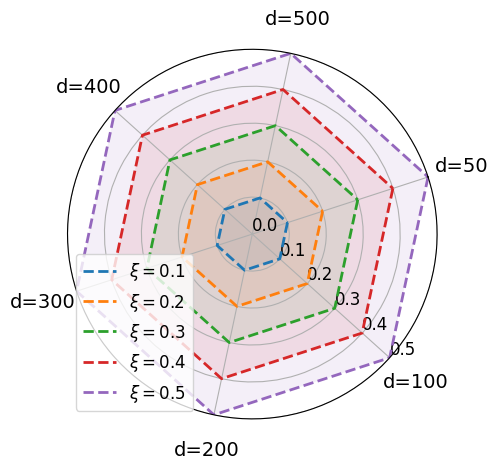
(a) $\min_{l\in[L-1],K+1\leq i\leq d-K}\;\sigma_{i}(\bm{W}_{l})$

(b) $\max_{l\in[L-1],K+1\leq i\leq d-K}\;\sigma_{i}(\bm{W}_{l})$

Figure 14: Approximate low-rankness hold universally across different training and network configurations. The experimental setup is deferred to Section 5.2.1. For each figure, the vertex of each polygon denotes the singular value of the weights for each $d$ and $\xi$. As we observe, for each fixed $\xi$, the polygon is a hexagon, implying that the singular values are approximately equal and independent of the network width $d$. Second, the singular values grow when the initialization scale $\xi$ increases and also confirms 1 that $\varepsilon=\xi$. Moreover, we conclude that $\sigma_{\min}\approx\sigma_{\max}$ when comparing (a) and (b). Therefore, we can see that both the minimum and maximum singular values remain unchanged, demonstrating that the GD operates only within a 2K-dimensional invariant subspace.

Appendix C Extra Experiments

Here, we provide more experimental results for validating the low-rankness property in 2 of trained weights in DLN. To validate the low-rankness assumption, we train 4-layer DLNs using the orthogonal initialization with width $d\in\left\{50,100,200,300,400,500\right\}$ and initialization scale $\xi\in\left\{0.1,0.2,0.3,0.4,0.5\right\}$. The training setting is the same with Section 5.2. For the weights $\left\{\bm{W}_{l}\right\}_{l=1}^{L-1}$ of each network that have been trained until convergence, we plot

$$\text{minimum singular value}\quad\sigma_{\min}\; :=\;\min_{K+1\leq i\leq d-K,\;l\in[L-1]}\sigma_{i}(\bm{W}_{l}),$$

$$\text{maximum singular value}\quad\sigma_{\max}; :=\;\max_{K+1\leq i\leq d-K,\;l\in[L-1]}\sigma_{i}(\bm{W}_{l}).$$

The results are shown in Figure 14. Here, for each $l\in[L-1]$, we assume that $\sigma_{1}(\bm{W}_{l})\geq\sigma_{2}(\bm{W}_{l})\geq\cdots\geq\sigma_{d}(\bm{W}_{l})$. For each figure, the vertex of each polygon denotes the singular value of the weights for each $d$ and $\xi$. As we observe, for each fixed $\xi$, the polygon is a hexagon, implying that the singular values are approximately equal and independent of the network width $d$. Second, the singular values grow when the initialization scale $\xi$ increases and also confirms 1 that $\varepsilon=\xi$. Moreover, we conclude that $\sigma_{\min}\approx\sigma_{\max}$ when comparing Figure 14(a) and Figure 14(b). Therefore, we can see that both the minimum and maximum singular values remain unchanged, demonstrating that the GD operates only within a 2K-dimensional invariant subspace.

References

• AB [17] Guillaume Alain and Yoshua Bengio. Understanding intermediate layers using linear classifier probes. In International Conference on Learning Representations, 2017.
• ACGH [18] Sanjeev Arora, Nadav Cohen, Noah Golowich, and Wei Hu. A convergence analysis of gradient descent for deep linear neural networks. In International Conference on Learning Representations, 2018.
• ACH [18] Sanjeev Arora, Nadav Cohen, and Elad Hazan. On the optimization of deep networks: Implicit acceleration by overparameterization. In International Conference on Machine Learning, pages 244–253. PMLR, 2018.
• ACHL [19] Sanjeev Arora, Nadav Cohen, Wei Hu, and Yuping Luo. Implicit regularization in deep matrix factorization. Advances in Neural Information Processing Systems, 32, 2019.
• ADH+ [19] Sanjeev Arora, Simon Du, Wei Hu, Zhiyuan Li, and Ruosong Wang. Fine-grained analysis of optimization and generalization for overparameterized two-layer neural networks. In International Conference on Machine Learning, pages 322–332. PMLR, 2019.
• AGM [14] Sanjeev Arora, Rong Ge, and Ankur Moitra. New algorithms for learning incoherent and overcomplete dictionaries. In Conference on Learning Theory, pages 779–806. PMLR, 2014.
• ALMZ [19] Alessio Ansuini, Alessandro Laio, Jakob H Macke, and Davide Zoccolan. Intrinsic dimension of data representations in deep neural networks. Advances in Neural Information Processing Systems, 32, 2019.
• AP [20] Ben Adlam and Jeffrey Pennington. The neural tangent kernel in high dimensions: Triple descent and a multi-scale theory of generalization. In International Conference on Machine Learning, pages 74–84. PMLR, 2020.
• AZL [19] Zeyuan Allen-Zhu and Yuanzhi Li. What can resnet learn efficiently, going beyond kernels? Advances in Neural Information Processing Systems, 32, 2019.
• AZL [23] Zeyuan Allen-Zhu and Yuanzhi Li. Backward feature correction: How deep learning performs deep (hierarchical) learning. In The Thirty Sixth Annual Conference on Learning Theory, pages 4598–4598. PMLR, 2023.
• AZLS [19] Zeyuan Allen-Zhu, Yuanzhi Li, and Zhao Song. A convergence theory for deep learning via over-parameterization. In International Conference on Machine Learning, pages 242–252. PMLR, 2019.
• BBSS [22] Alberto Bietti, Joan Bruna, Clayton Sanford, and Min Jae Song. Learning single-index models with shallow neural networks. Advances in Neural Information Processing Systems, 35:9768–9783, 2022.
• BHMM [19] Mikhail Belkin, Daniel Hsu, Siyuan Ma, and Soumik Mandal. Reconciling modern machine-learning practice and the classical bias–variance trade-off. Proceedings of the National Academy of Sciences, 116(32):15849–15854, 2019.
• BLLT [20] Peter L Bartlett, Philip M Long, Gábor Lugosi, and Alexander Tsigler. Benign overfitting in linear regression. Proceedings of the National Academy of Sciences, 117(48):30063–30070, 2020.
• BPVF [22] Etienne Boursier, Loucas Pillaud-Vivien, and Nicolas Flammarion. Gradient flow dynamics of shallow relu networks for square loss and orthogonal inputs. In Advances in Neural Information Processing Systems, 2022.
• BRTW [22] Bubacarr Bah, Holger Rauhut, Ulrich Terstiege, and Michael Westdickenberg. Learning deep linear neural networks: Riemannian gradient flows and convergence to global minimizers. Information and Inference: A Journal of the IMA, 11(1):307–353, 2022.
• BSD [22] Ido Ben-Shaul and Shai Dekel. Nearest class-center simplification through intermediate layers. In Topological, Algebraic and Geometric Learning Workshops 2022, pages 37–47. PMLR, 2022.
• CBL+ [20] Minshuo Chen, Yu Bai, Jason D Lee, Tuo Zhao, Huan Wang, Caiming Xiong, and Richard Socher. Towards understanding hierarchical learning: Benefits of neural representations. Advances in Neural Information Processing Systems, 33:22134–22145, 2020.
• CFN+ [22] Mayee Chen, Daniel Y Fu, Avanika Narayan, Michael Zhang, Zhao Song, Kayvon Fatahalian, and Christopher Ré. Perfectly balanced: Improving transfer and robustness of supervised contrastive learning. In International Conference on Machine Learning, pages 3090–3122. PMLR, 2022.
• CH [21] Xinlei Chen and Kaiming He. Exploring simple siamese representation learning. 2021 IEEE/CVF Conference on Computer Vision and Pattern Recognition (CVPR), pages 15745–15753, 2021.
• CKNH [20] Ting Chen, Simon Kornblith, Mohammad Norouzi, and Geoffrey Hinton. A simple framework for contrastive learning of visual representations. In International Conference on Machine Learning, pages 1597–1607. PMLR, 2020.
• CL [23] Niladri S Chatterji and Philip M Long. Deep linear networks can benignly overfit when shallow ones do. Journal of Machine Learning Research, 24(117):1–39, 2023.
• CLB [22] Niladri S Chatterji, Philip M Long, and Peter L Bartlett. The interplay between implicit bias and benign overfitting in two-layer linear networks. The Journal of Machine Learning Research, 23(1):12062–12109, 2022.
• CYY+ [22] Kwan Ho Ryan Chan, Yaodong Yu, Chong You, Haozhi Qi, John Wright, and Yi Ma. Redunet: A white-box deep network from the principle of maximizing rate reduction. Journal of Machine Learning Research, 23(114):1–103, 2022.
• CYZ [22] Yixiong Chen, Alan Yuille, and Zongwei Zhou. Which layer is learning faster? a systematic exploration of layer-wise convergence rate for deep neural networks. In The Eleventh International Conference on Learning Representations, 2022.
• CZLG [23] Yuan Cao, Difan Zou, Yuanzhi Li, and Quanquan Gu. The implicit bias of batch normalization in linear models and two-layer linear convolutional neural networks. In Gergely Neu and Lorenzo Rosasco, editors, Proceedings of Thirty Sixth Conference on Learning Theory, volume 195 of Proceedings of Machine Learning Research, pages 5699–5753. PMLR, 12–15 Jul 2023.
• DCT+ [23] Xili Dai, Ke Chen, Shengbang Tong, Jingyuan Zhang, Xingjian Gao, Mingyang Li, Druv Pai, Yuexiang Zhai, XIaojun Yuan, Heung-Yeung Shum, et al. Closed-loop transcription via convolutional sparse coding. arXiv preprint arXiv:2302.09347, 2023.
• DE [03] David L Donoho and Michael Elad. Optimally sparse representation in general (nonorthogonal) dictionaries via l1 minimization. Proceedings of the National Academy of Sciences, 100(5):2197–2202, 2003.
• DH [19] Simon Du and Wei Hu. Width provably matters in optimization for deep linear neural networks. In International Conference on Machine Learning, pages 1655–1664. PMLR, 2019.
• DHL [18] Simon S Du, Wei Hu, and Jason D Lee. Algorithmic regularization in learning deep homogeneous models: Layers are automatically balanced. Advances in Neural Information Processing Systems, 31, 2018.
• DLS [22] Alexandru Damian, Jason Lee, and Mahdi Soltanolkotabi. Neural networks can learn representations with gradient descent. In Conference on Learning Theory, pages 5413–5452. PMLR, 2022.
• DNT+ [23] Hien Dang, Tan Minh Nguyen, Tho Tran, Hung The Tran, Hung Tran, and Nhat Ho. Neural collapse in deep linear networks: From balanced to imbalanced data. In International Conference on Machine Learning, 2023.
• DZPS [18] Simon S Du, Xiyu Zhai, Barnabas Poczos, and Aarti Singh. Gradient descent provably optimizes over-parameterized neural networks. In International Conference on Learning Representations, 2018.
• EDLM [22] Utku Evci, Vincent Dumoulin, Hugo Larochelle, and Michael C Mozer. Head2toe: Utilizing intermediate representations for better transfer learning. In International Conference on Machine Learning, pages 6009–6033. PMLR, 2022.
• Eft [20] Armin Eftekhari. Training linear neural networks: Non-local convergence and complexity results. In International Conference on Machine Learning, pages 2836–2847. PMLR, 2020.
• ERR+ [19] Andre Esteva, Alexandre Robicquet, Bharath Ramsundar, Volodymyr Kuleshov, Mark DePristo, Katherine Chou, Claire Cui, Greg Corrado, Sebastian Thrun, and Jeff Dean. A guide to deep learning in healthcare. Nature Medicine, 25(1):24–29, 2019.
• FHLS [21] Cong Fang, Hangfeng He, Qi Long, and Weijie J Su. Exploring deep neural networks via layer-peeled model: Minority collapse in imbalanced training. Proceedings of the National Academy of Sciences, 118(43), 2021.
• FVB+ [23] Spencer Frei, Gal Vardi, Peter Bartlett, Nathan Srebro, and Wei Hu. Implicit bias in leaky relu networks trained on high-dimensional data. In The Eleventh International Conference on Learning Representations, 2023.
• GAS [20] Shuxuan Guo, Jose M Alvarez, and Mathieu Salzmann. Expandnets: Linear over-parameterization to train compact convolutional networks. Advances in Neural Information Processing Systems, 33:1298–1310, 2020.
• GB [10] Xavier Glorot and Yoshua Bengio. Understanding the difficulty of training deep feedforward neural networks. In Proceedings of the thirteenth international conference on artificial intelligence and statistics, pages 249–256. JMLR Workshop and Conference Proceedings, 2010.
• GBLJ [19] Gauthier Gidel, Francis Bach, and Simon Lacoste-Julien. Implicit regularization of discrete gradient dynamics in linear neural networks. Advances in Neural Information Processing Systems, 32, 2019.
• GGBS [22] Tomer Galanti, Liane Galanti, and Ido Ben-Shaul. On the implicit bias towards minimal depth of deep neural networks. arXiv preprint arXiv:2202.09028, 2022.
• GGH [22] Tomer Galanti, András György, and Marcus Hutter. On the role of neural collapse in transfer learning. In International Conference on Learning Representations, 2022.
• GLPR [23] Borjan Geshkovski, Cyril Letrouit, Yury Polyanskiy, and Philippe Rigollet. The emergence of clusters in self-attention dynamics. arXiv preprint arXiv:2305.05465, 2023.
• GWB+ [17] Suriya Gunasekar, Blake E Woodworth, Srinadh Bhojanapalli, Behnam Neyshabur, and Nati Srebro. Implicit regularization in matrix factorization. Advances in Neural Information Processing Systems, 30, 2017.
• HB [20] Like Hui and Mikhail Belkin. Evaluation of neural architectures trained with square loss vs cross-entropy in classification tasks. In International Conference on Learning Representations, 2020.
• HBN [22] Like Hui, Mikhail Belkin, and Preetum Nakkiran. Limitations of neural collapse for understanding generalization in deep learning. arXiv preprint arXiv:2202.08384, 2022.
• HM [16] Moritz Hardt and Tengyu Ma. Identity matters in deep learning. In International Conference on Learning Representations, 2016.
• HMZ+ [23] Minyoung Huh, Hossein Mobahi, Richard Zhang, Brian Cheung, Pulkit Agrawal, and Phillip Isola. The low-rank simplicity bias in deep networks. Transactions on Machine Learning Research, 2023.
• HPD [21] XY Han, Vardan Papyan, and David L Donoho. Neural collapse under mse loss: Proximity to and dynamics on the central path. In International Conference on Learning Representations, 2021.
• HS [23] Hangfeng He and Weijie J Su. A law of data separation in deep learning. Proceedings of the National Academy of Sciences, 120(36):e2221704120, 2023.
• HXAP [20] Wei Hu, Lechao Xiao, Ben Adlam, and Jeffrey Pennington. The surprising simplicity of the early-time learning dynamics of neural networks. Advances in Neural Information Processing Systems, 33:17116–17128, 2020.
• HXP [19] Wei Hu, Lechao Xiao, and Jeffrey Pennington. Provable benefit of orthogonal initialization in optimizing deep linear networks. In International Conference on Learning Representations, 2019.
• HY [20] Jiaoyang Huang and Horng-Tzer Yau. Dynamics of deep neural networks and neural tangent hierarchy. In International Conference on Machine Learning, pages 4542–4551. PMLR, 2020.
• HZRS [15] Kaiming He, Xiangyu Zhang, Shaoqing Ren, and Jian Sun. Delving deep into rectifiers: Surpassing human-level performance on imagenet classification. In Proceedings of the IEEE International Conference on Computer Vision, pages 1026–1034, 2015.
• HZRS [16] Kaiming He, Xiangyu Zhang, Shaoqing Ren, and Jian Sun. Deep residual learning for image recognition. In Proceedings of the IEEE conference on computer vision and pattern recognition, pages 770–778, 2016.
• IS [15] Sergey Ioffe and Christian Szegedy. Batch normalization: Accelerating deep network training by reducing internal covariate shift. In International Conference on Machine Learning, pages 448–456. PMLR, 2015.
• JGH [18] Arthur Jacot, Franck Gabriel, and Clément Hongler. Neural tangent kernel: Convergence and generalization in neural networks. Advances in Neural Information Processing Systems, 31, 2018.
• JLZ+ [22] Wenlong Ji, Yiping Lu, Yiliang Zhang, Zhun Deng, and Weijie J Su. An unconstrained layer-peeled perspective on neural collapse. In International Conference on Learning Representations, 2022.
• JT [18] Ziwei Ji and Matus Telgarsky. Gradient descent aligns the layers of deep linear networks. In International Conference on Learning Representations, 2018.
• JT [19] Ziwei Ji and Matus Telgarsky. The implicit bias of gradient descent on nonseparable data. In Conference on Learning Theory, pages 1772–1798. PMLR, 2019.
• Kaw [16] Kenji Kawaguchi. Deep learning without poor local minima. Advances in Neural Information Processing Systems, 29, 2016.
• KCLN [21] Simon Kornblith, Ting Chen, Honglak Lee, and Mohammad Norouzi. Why do better loss functions lead to less transferable features? Advances in Neural Information Processing Systems, 34:28648–28662, 2021.
• KH+ [09] Alex Krizhevsky, Geoffrey Hinton, et al. Learning multiple layers of features from tiny images. 2009.
• KSH [12] Alex Krizhevsky, Ilya Sutskever, and Geoffrey E Hinton. Imagenet classification with deep convolutional neural networks. Advances in Neural Information Processing Systems, 25, 2012.
• KTB [23] Vignesh Kothapalli, Tom Tirer, and Joan Bruna. A neural collapse perspective on feature evolution in graph neural networks. arXiv preprint arXiv:2307.01951, 2023.
• KYMG [22] Daniel Kunin, Atsushi Yamamura, Chao Ma, and Surya Ganguli. The asymmetric maximum margin bias of quasi-homogeneous neural networks. In The Eleventh International Conference on Learning Representations, 2022.
• KZS+ [23] Soo Min Kwon, Zekai Zhang, Dogyoon Song, Laura Balzano, and Qing Qu. Compressing overparameterized deep models by harnessing low-dimensional learning dynamics. arXiv preprint, 2023.
• LB [18] Thomas Laurent and James Brecht. Deep linear networks with arbitrary loss: All local minima are global. In International Conference on Machine Learning, pages 2902–2907. PMLR, 2018.
• LBH [15] Yann LeCun, Yoshua Bengio, and Geoffrey Hinton. Deep learning. Nature, 521(7553):436–444, 2015.
• LG [18] Andrew K Lampinen and Surya Ganguli. An analytic theory of generalization dynamics and transfer learning in deep linear networks. In International Conference on Learning Representations, 2018.
• LH [17] Ilya Loshchilov and Frank Hutter. SGDR: Stochastic gradient descent with warm restarts. In International Conference on Learning Representations, 2017.
• LK [17] Haihao Lu and Kenji Kawaguchi. Depth creates no bad local minima. arXiv preprint arXiv:1702.08580, 2017.
• LL [19] Kaifeng Lyu and Jian Li. Gradient descent maximizes the margin of homogeneous neural networks. arXiv preprint arXiv:1906.05890, 2019.
• LLZ+ [22] Xiao Li, Sheng Liu, Jinxin Zhou, Xinyu Lu, Carlos Fernandez-Granda, Zhihui Zhu, and Qing Qu. Principled and efficient transfer learning of deep models via neural collapse. arXiv preprint arXiv:2212.12206, 2022.
• LWLQ [23] Pengyu Li, Yutong Wang, Xiao Li, and Qing Qu. Neural collapse in multi-label learning with pick-all-label loss. arXiv preprint arXiv:2310.15903, 2023.
• MHSG [18] Leland McInnes, John Healy, Nathaniel Saul, and Lukas Groberger. Umap: Uniform manifold approximation and projection. Journal of Open Source Software, 3(29):861, 2018.
• MKAS [21] Eran Malach, Pritish Kamath, Emmanuel Abbe, and Nathan Srebro. Quantifying the benefit of using differentiable learning over tangent kernels. In International Conference on Machine Learning, pages 7379–7389. PMLR, 2021.
• MOI+ [23] Wojciech Masarczyk, Mateusz Ostaszewski, Ehsan Imani, Razvan Pascanu, Piotr Miłoś, and Tomasz Trzciński. The tunnel effect: Building data representations in deep neural networks. arXiv preprint arXiv:2305.19753, 2023.
• MPP [20] Dustin G Mixon, Hans Parshall, and Jianzong Pi. Neural collapse with unconstrained features. arXiv preprint arXiv:2011.11619, 2020.
• MTS [22] Yi Ma, Doris Tsao, and Heung-Yeung Shum. On the principles of parsimony and self-consistency for the emergence of intelligence. Frontiers of Information Technology & Electronic Engineering, 23(9):1298–1323, 2022.
• MTVM [21] Hancheng Min, Salma Tarmoun, René Vidal, and Enrique Mallada. On the explicit role of initialization on the convergence and implicit bias of overparametrized linear networks. In International Conference on Machine Learning, pages 7760–7768. PMLR, 2021.
• Ney [17] Behnam Neyshabur. Implicit regularization in deep learning. arXiv preprint arXiv:1709.01953, 2017.
• Nic [21] Eshaan Nichani. An Empirical and Theoretical Analysis of the Role of Depth in Convolutional Neural Networks. PhD thesis, Massachusetts Institute of Technology, 2021.
• NLG+ [19] Mor Shpigel Nacson, Jason Lee, Suriya Gunasekar, Pedro Henrique Pamplona Savarese, Nathan Srebro, and Daniel Soudry. Convergence of gradient descent on separable data. In The 22nd International Conference on Artificial Intelligence and Statistics, pages 3420–3428. PMLR, 2019.
• NRT [21] Gabin Maxime Nguegnang, Holger Rauhut, and Ulrich Terstiege. Convergence of gradient descent for learning linear neural networks. arXiv preprint arXiv:2108.02040, 2021.
• PHD [20] Vardan Papyan, XY Han, and David L Donoho. Prevalence of neural collapse during the terminal phase of deep learning training. Proceedings of the National Academy of Sciences, 117(40):24652–24663, 2020.
• PL [20] Mary Phuong and Christoph H Lampert. The inductive bias of relu networks on orthogonally separable data. In International Conference on Learning Representations, 2020.
• PSG [18] Jeffrey Pennington, Samuel Schoenholz, and Surya Ganguli. The emergence of spectral universality in deep networks. In International Conference on Artificial Intelligence and Statistics, pages 1924–1932. PMLR, 2018.
• QZL+ [20] Qing Qu, Yuexiang Zhai, Xiao Li, Yuqian Zhang, and Zhihui Zhu. Geometric analysis of nonconvex optimization landscapes for overcomplete learning. In International Conference on Learning Representations, 2020.
• RFA+ [19] Stefano Recanatesi, Matthew Farrell, Madhu Advani, Timothy Moore, Guillaume Lajoie, and Eric Shea-Brown. Dimensionality compression and expansion in deep neural networks. arXiv preprint arXiv:1906.00443, 2019.
• RLGP [23] Akshay Rangamani, Marius Lindegaard, Tomer Galanti, and Tomaso A Poggio. Feature learning in deep classifiers through intermediate neural collapse. In International Conference on Machine Learning, pages 28729–28745. PMLR, 2023.
• Shi [22] Yeonjong Shin. Effects of depth, width, and initialization: A convergence analysis of layer-wise training for deep linear neural networks. Analysis and Applications, 20(01):73–119, 2022.
• SHN+ [18] Daniel Soudry, Elad Hoffer, Mor Shpigel Nacson, Suriya Gunasekar, and Nathan Srebro. The implicit bias of gradient descent on separable data. The Journal of Machine Learning Research, 19(1):2822–2878, 2018.
• SMG [13] Andrew M Saxe, James L McClelland, and Surya Ganguli. Exact solutions to the nonlinear dynamics of learning in deep linear neural networks. arXiv preprint arXiv:1312.6120, 2013.
• SMG [19] Andrew M Saxe, James L McClelland, and Surya Ganguli. A mathematical theory of semantic development in deep neural networks. Proceedings of the National Academy of Sciences, 116(23):11537–11546, 2019.
• SML [23] Peter Súkeník, Marco Mondelli, and Christoph Lampert. Deep neural collapse is provably optimal for the deep unconstrained features model. arXiv preprint arXiv:2305.13165, 2023.
• SQW [16] Ju Sun, Qing Qu, and John Wright. Complete dictionary recovery over the sphere i: Overview and the geometric picture. IEEE Transactions on Information Theory, 63(2):853–884, 2016.
• SS [90] Gilbert W Stewart and Ji-guang Sun. Matrix perturbation theory. 1990.
• STR+ [20] Harshay Shah, Kaustav Tamuly, Aditi Raghunathan, Prateek Jain, and Praneeth Netrapalli. The pitfalls of simplicity bias in neural networks. Advances in Neural Information Processing Systems, 33:9573–9585, 2020.
• Sut [23] Ilya Sutskever. A Theory of Unsupervised Learning, 2023. https://www.youtube.com/watch?v=AKMuA_TVz3A.
• SVL [14] Ilya Sutskever, Oriol Vinyals, and Quoc V Le. Sequence to sequence learning with neural networks. Advances in Neural Information Processing Systems, 27, 2014.
• SZ [15] Karen Simonyan and Andrew Zisserman. Very deep convolutional networks for large-scale image recognition. In International Conference on Learning Representations, 2015.
• SZL [23] Ravid Shwartz-Ziv and Yann LeCun. To compress or not to compress–self-supervised learning and information theory: A review. arXiv preprint arXiv:2304.09355, 2023.
• TB [22] Tom Tirer and Joan Bruna. Extended unconstrained features model for exploring deep neural collapse. In International Conference on Machine Learning, pages 21478–21505. PMLR, 2022.
• TFHV [21] Salma Tarmoun, Guilherme Franca, Benjamin D Haeffele, and Rene Vidal. Understanding the dynamics of gradient flow in overparameterized linear models. In International Conference on Machine Learning, pages 10153–10161. PMLR, 2021.
• THNW [23] Tom Tirer, Haoxiang Huang, and Jonathan Niles-Weed. Perturbation analysis of neural collapse. In International Conference on Machine Learning, pages 34301–34329. PMLR, 2023.
• VPCL [18] Guillermo Valle-Perez, Chico Q Camargo, and Ard A Louis. Deep learning generalizes because the parameter-function map is biased towards simple functions. In International Conference on Learning Representations, 2018.
• VSP+ [17] Ashish Vaswani, Noam Shazeer, Niki Parmar, Jakob Uszkoreit, Llion Jones, Aidan N Gomez, Lukasz Kaiser, and Illia Polosukhin. Attention is all you need. Advances in Neural Information Processing Systems, 30, 2017.
• WLY+ [22] Peng Wang, Huikang Liu, Can Yaras, Laura Balzano, and Qing Qu. Linear convergence analysis of neural collapse with unconstrained features. In OPT 2022: Optimization for Machine Learning (NeurIPS 2022 Workshop), 2022.
• XBSD+ [18] Lechao Xiao, Yasaman Bahri, Jascha Sohl-Dickstein, Samuel Schoenholz, and Jeffrey Pennington. Dynamical isometry and a mean field theory of cnns: How to train 10,000-layer vanilla convolutional neural networks. In International Conference on Machine Learning, pages 5393–5402. PMLR, 2018.
• XQP+ [22] Shuo Xie, Jiahao Qiu, Ankita Pasad, Li Du, Qing Qu, and Hongyuan Mei. Hidden state variability of pretrained language models can guide computation reduction for transfer learning. In The 2022 Conference on Empirical Methods in Natural Language Processing, 2022.
• XRV [17] Han Xiao, Kashif Rasul, and Roland Vollgraf. Fashion-mnist: a novel image dataset for benchmarking machine learning algorithms. arXiv preprint arXiv:1708.07747, 2017.
• YBP+ [23] Yaodong Yu, Sam Buchanan, Druv Pai, Tianzhe Chu, Ziyang Wu, Shengbang Tong, Benjamin D Haeffele, and Yi Ma. White-box transformers via sparse rate reduction. arXiv preprint arXiv:2306.01129, 2023.
• YCBL [14] Jason Yosinski, Jeff Clune, Yoshua Bengio, and Hod Lipson. How transferable are features in deep neural networks? Advances in neural information processing systems, 27, 2014.
• YCY+ [20] Yaodong Yu, Kwan Ho Ryan Chan, Chong You, Chaobing Song, and Yi Ma. Learning diverse and discriminative representations via the principle of maximal coding rate reduction. Advances in Neural Information Processing Systems, 33:9422–9434, 2020.
• YWH+ [23] Can Yaras, Peng Wang, Wei Hu, Zhihui Zhu, Laura Balzano, and Qing Qu. The law of parsimony in gradient descent for learning deep linear networks. arXiv preprint arXiv:2306.01154, 2023.
• YWZ+ [22] Can Yaras, Peng Wang, Zhihui Zhu, Laura Balzano, and Qing Qu. Neural collapse with normalized features: A geometric analysis over the riemannian manifold. In Advances in Neural Information Processing Systems, 2022.
• ZBS [22] Chiyuan Zhang, Samy Bengio, and Yoram Singer. Are all layers created equal? The Journal of Machine Learning Research, 23(1):2930–2957, 2022.
• ZDZ+ [21] Zhihui Zhu, Tianyu Ding, Jinxin Zhou, Xiao Li, Chong You, Jeremias Sulam, and Qing Qu. A geometric analysis of neural collapse with unconstrained features. Advances in Neural Information Processing Systems, 34, 2021.
• ZLD+ [22] Jinxin Zhou, Xiao Li, Tianyu Ding, Chong You, Qing Qu, and Zhihui Zhu. On the optimization landscape of neural collapse under mse loss: Global optimality with unconstrained features. In International Conference on Machine Learning, pages 27179–27202. PMLR, 2022.
• ZYL+ [20] Yuexiang Zhai, Zitong Yang, Zhenyu Liao, John Wright, and Yi Ma. Complete dictionary learning via l 4-norm maximization over the orthogonal group. The Journal of Machine Learning Research, 21(1):6622–6689, 2020.
• ZYL+ [22] Jinxin Zhou, Chong You, Xiao Li, Kangning Liu, Sheng Liu, Qing Qu, and Zhihui Zhu. Are all losses created equal: A neural collapse perspective. Advances in Neural Information Processing Systems, 35:31697–31710, 2022.