Safe and Efficient Trajectory Optimization for Autonomous Vehicles using B-Spline with Incremental Path Flattening

Abstract

B-spline-based trajectory optimization is widely used for robot navigation due to its computational efficiency and convex-hull property (ensures dynamic feasibility), especially as quadrotors, which have circular body shapes (enable efficient movement) and freedom to move each axis (enables convex-hull property utilization). However, using the B-spline curve for trajectory optimization is challenging for autonomous vehicles (AVs)because of their vehicle kinodynamics (rectangular body shapes and constraints to move each axis). In this study, we propose a novel trajectory optimization approach for AVs to circumvent this difficulty using an incremental path flattening (IPF), a disc type swept volume (SV)estimation method, and kinodynamic feasibility constraints. IPF is a new method that can find a collision-free path for AVs by flattening path and reducing SV using iteratively increasing curvature penalty around vehicle collision points. Additionally, we develop a disc type SV estimation method to reduce SV over-approximation and enable AVs to pass through a narrow corridor efficiently. Furthermore, a clamped B-spline curvature constraint, which simplifies a B-spline curvature constraint, is added to dynamical feasibility constraints (e.g., velocity and acceleration) for obtaining the kinodynamic feasibility constraints. Our experimental results demonstrate that our method outperforms state-of-the-art baselines in various simulated environments. We also conducted a real-world experiment using an AV, and our results validate the simulated tracking performance of the proposed approach.

I INTRODUCTION

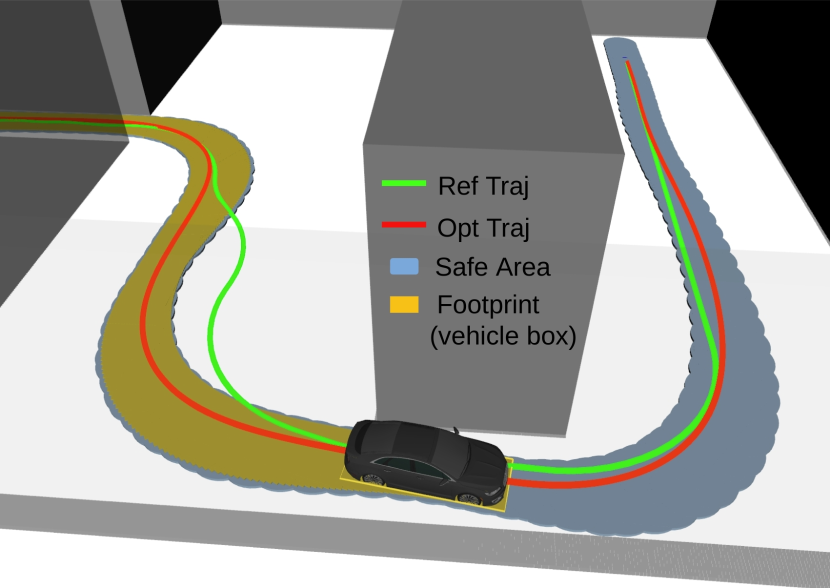
Figure 1: Proposed algorithm. The algorithm can generate an optimized trajectory (red) that allows the vehicle to pass through a narrow corridor based on a reference path (hybrid $\text{A}^{*}$, green). The footprint (yellow) of the vehicle box inside of the safe area (blue) generated by the proposed SV estimation method shows that the proposed algorithm can generate a safe, tractable trajectory. The simulated video and more examples can be found at https://youtu.be/7bhxfuhAqos.

Extensive researches have focused on trajectory optimization for AVs to generate safe, efficient, and robust trajectories. Trajectory optimization algorithms are primarily classified as path-velocity decoupled methods [1, 2, 3], or coupled methods [4, 5, 6]. Decoupled methods sequentially and iteratively optimize the path and velocity and require many path and velocity iterations to generate an efficient trajectory. Despite this drawback, such methods are computationally efficient because they benefit from a two-dimensional breakdown (x-y and s-t domains), which enables their widespread use for trajectory optimization.

Coupled methods can consider path and velocity constraints simultaneously but are usually computationally expensive because of their higher-dimensional (x-y-t) optimization. A coupled trajectory optimization problem is commonly described as an optimal-control problem (OCP), which entails finding the control variables of a dynamic system over a future time horizon. An OCP has many advantages, including the modeling of complex dynamic systems and the flexible handling of optimal controls under their boundary conditions [7, 8]. However, the modeling complexity of an OCP (e.g., vehicle kinematics, and numerous control variables) can degrade computational efficiency.

B-spline-based optimization methods are promising approaches to trajectory optimization; such a method is computationally efficient because it changes the entire B-spline curve shape using a small number of control points. Therefore, we develop a trajectory optimization method for AVs using a fast B-spline-based optimization algorithm called ESDF-free gradient-based local planning framework (EGO-Planner)[9]. EGO-Planner is robust and computationally efficient because it uses repulsive force from obstacles instead of using euclidean signed distance fields (ESDFs), which consumes a large part of the planning process time. The advantages of this algorithm ensure the robustness and high computational efficiency of our proposed method.

However, AVs are difficult to use the EGO-Planner, which is designed for quadrotors, because of their different body shapes and kinematics. Quadrotors [10, 11, 9] have circular body shapes, that can be covered by a fixed radius disc constraint and freedom to move each axis (x, y, and z), that enables to use the convex-hull property [12] (a B-spline curve is always contained in the convex-hull of its control polygon) of the B-spline curve to guarantee their dynamical feasibility constraints (e.g., velocity, acceleration, and jerk) because the derivative of a B-spline curve is also a B-spline curve. AVs have rectangular body shapes, that lead to overly conservative move if they are covered by a fixed radius disc constraint and their constraints in longitudinal and lateral motion, which cannot guarantee their dynamical feasibility constraints by the convex-hull property.

The proposed trajectory optimization algorithm uses the B-spline curve with incremental path flattening (IPF)and a new SV estimation method to generate a safe and efficient trajectory for AVs by minimizing the SV of the vehicle’s rectangular body shape (Fig. 1). IPF is a new method that iteratively flattens the path around a vehicle’s collision points by increasing the path curvature weight. It allows the proposed algorithm to use a B-spline curve to find a collision-free path by reducing the SV. The SV should be considered for safe trajectory optimization to prevent the well-known corner-cutting problem [13], which is normally handled using a large enough number of control points [14, 7]. Our disc type SV estimation method can minimize the over-approximation of SV, thus expanding the problem solution area (e.g., narrow corridor), by calculating the number of discs and the minimum disc radius needed to cover the actual vehicle SV. Furthermore, a clamped B-spline curvature constraint is used to simplify the B-spline curvature constraint. The kinodynamic feasibility constraints (velocity, acceleration, and curvature) allow the B-spline curve to plan a kinodynamically feasible trajectory for AVs.

The main contributions of this paper are summarized as follows:

• We propose a novel, efficient B-spline-based trajectory optimization algorithm that incorporates vehicle kinodynamcis.

• We propose an IPF and a new disc type SV estimation method that enables an AV to move efficiently (e.g. passing through a narrow corridor) by minimizing the over-approximation of the SV.

• We integrate kinodynamic constraints, namely, curvature, velocity, and acceleration into B-spline-based trajectory optimization to generate a tractable trajectory for an AV.

• The efficiency, robustness, and tracking performance of the proposed trajectory optimization approach are validated through numerous driving tasks in comparison with state-of-the-art (SOTA)algorithms.

II RELATED WORK

II-A Safe Trajectory Optimization for AVs

The major concern in AV trajectory optimization is the generation of collision-free trajectories considering vehicle kinematics. References [15, 16] propose nonlinear programming (NLP)methods with direct obstacle-to-obstacle collision avoidance constraints; these methods include the triangle area criterion method [17] and signed distance fields [18]. However, in these approaches, most constraints are unused because not all obstacles collide with a vehicle simultaneously. The numerous redundant constraints can significantly slow the system down.

To overcome this issue, researchers [14, 19, 20, 21] generate safe convex corridors, which are substantially advantageous in terms of computational efficiency because the number of obstacles is irrelevant. Nevertheless, these algorithms suffer from the corner-cutting problem [13]. This is prevented using a large enough number of control points [14, 7], which can prolong computation, or using various methods to estimate the SV [22, 23, 24] between the control points of a trajectory. However, they can lead to conservative SV s because they use convex polygons, thus creating redundant regions at a curve. Therefore, a safe and efficient SV with minimal over-approximation is vital in the generation of a feasible trajectory for AVs to increase the robustness of the optimization in complex environments.

II-B B-Spline Based Trajectory Optimization

B-spline-based trajectory optimization algorithms [10, 11] for quadrotors generate efficient, dynamically feasible trajectories with the computational efficiency caused by the convex-hull property of B-spline curve. EGO-Planner [9] accelerates computation by generating gradient information using repulsive force from obstacles instead of ESDFs.

Because of the benefits of B-spline curve, numerous researchers have attempted to use them for AVs. References [25, 26] use B-spline curve to generate curvature-continuous paths for AVs, but velocity is not considered in path planning. Reference [27] manipulates B-spline curve using their local-control property for collision avoidance in spatial-temporal path planning. Reference [28] uses piecewise B$\acute{e}$zier curves, which have similar properties to B-spline curve, to optimize a trajectory in a spatio-temporal semantic corridor. Reference [29] uses B-spline curve for string stability in cooperative driving. However, these algorithms [27, 28, 29] mostly use B-spline curve for longitudinal trajectory planning without considering vehicle kinematics for lateral motion. Reference [30] uses B-spline curve for longitudinal and lateral trajectory planning by utilizing a hyperplane as the collision avoidance constraint, but this method imposes overly conservative constraints by simplifying obstacle shapes such as into circles. The computational inefficiency of this approach is the same as that of the obstacle-to-obstacle collision avoidance method due to redundant constraints and the limited problem solution area caused by the over-approximation of the obstacle volume. Therefore, trajectory optimization should be formulated for safe, efficient, and robust autonomous driving.

Section III defines B-spline and SV estimation method. Section IV explains the overall trajectory optimization algorithm. The evaluation of this algorithm via simulation and real driving tests is explained in Sections V and VI. Finally, the conclusion is presented in Section VII.

III B-spline and SV Estimation Method

This section parameterized the B-spline and SV estimation method used for B-spline-based trajectory optimization (Section IV). We parameterize the B-spline primitives of [11] and [9] and then introduce the velocity, acceleration, and curvature of the B-spline curve. As for SV estimation method, discrete-time SV estimation method [8, 24] are summarized and a continuous-time SV estimation method is proposed.

III-A B-Spline Primitives

Initially, a collision-free trajectory $\Gamma$ satisfying the terminal constraints is given. The initial reference trajectory is parameterized to a uniform B-spline curve $\bm{\Phi}^{ref}$ with degree $p_{b}$, $N_{c}+1$ control points $\{\mathbf{Q}_{0},\mathbf{Q}_{1},\ldots,\mathbf{Q}_{N_{c}}\}$, and knot vectors $\{t_{0},t_{1},\ldots,t_{M}\}$, where $M=N_{c}+p_{b}+1$, $t_{m}\in\mathbb{R}$, and $t\in[t_{m},t_{m+1})\subset[t_{p_{b}},t_{M-p_{b}}]$. Every knot span $\Delta t=t_{m+1}-t_{m}$ is the same for a uniform B-spline curve and $t$ is normalized as $u=(t-t_{m})/\Delta t$. The control point $\mathbf{Q}_{i}$ is downgraded to $\mathbb{R}^{3}\rightarrow\mathbb{R}^{2}$ because AVs usually move in two-dimensional spaces (x, y), unlike quadrotors, which move in three-dimensional spaces (x, y, z). The convex-hull property of B-spline curve enables the derivatives of a B-spline curve to ensure the dynamic feasibility of the entire trajectory. Therefore, the derivatives of a B-spline curve can be formulated with the control points of velocity $\mathbf{V}_{i}$, acceleration $\mathbf{A}_{i}$, and jerk $\mathbf{J}_{i}$, which are obtained as

$$\mathbf{V}_{i}=\frac{\mathbf{Q}_{i+1}-\mathbf{Q}_{i}}{\Delta t},\mathbf{A}_{i}=\frac{\mathbf{V}_{i+1}-\mathbf{V}_{i}}{\Delta t},\mathbf{J}_{i}=\frac{\mathbf{A}_{i+1}-\mathbf{A}_{i}}{\Delta t}.$$ (1)

The position of a B-spline at time $t$ (normalized as $u$) can be evaluated using a matrix representation [31]:

$$\bm{p}_{t}=u^{\top}\mathbf{M}_{p_{b}+1}\bm{q}_{m},$$ (2)

$$u=[1\quad u\quad u^{2}\quad\ldots\quad u^{p_{b}}]^{\top},$$

$$\bm{q}_{m}=[\mathbf{Q}_{m-p_{b}}\quad\mathbf{Q}_{m-p_{b}+1}\quad\mathbf{Q}_{m-p_{b}+2}\quad\ldots\mathbf{Q}_{m}]^{\top},$$

where $\mathbf{M}_{p_{b}+1}$ is a constant matrix determined by $p_{b}$. In this work, $\bm{p}_{t}=(x_{t},y_{t})$ denotes the midpoint of the rear axle of the ego vehicle at time $t$, and the derivatives at time $t$ are velocity $\bm{v}_{t}=(v^{x}_{t},v^{y}_{t})$ and acceleration $\bm{a}_{t}=(a^{x}_{t},a^{y}_{t})$.

III-B Longitudinal and Lateral Velocity and Acceleration

Unlike quadrotors, which are free to move each axis (x, y, and z), AVs are constrained in both the longitudinal direction $s$ and the lateral direction $d$. Therefore, the B-spline derivatives in each direction should also be formulated. Because $\bm{p}_{t}$ is the midpoint of the rear axle of the ego vehicle at time $t$, we assume that the velocity $\bm{v}_{t}$ is always tangent to the vehicle path which means the lateral velocity is equal to zero. Acceleration in both directions $a^{\sigma}_{t}$ are calculated as

$$a^{s}_{t}=\|\bm{a}_{t}\|\cos(\theta^{(2)}_{t}-\theta^{(1)}_{t}),a^{d}_{t}=\|\bm{a}_{t}\|\sin(\theta^{(2)}_{t}-\theta^{(1)}_{t}),$$ (3)

where ${\sigma}\in\{s,d\}$, $\theta^{(1)}_{t}=\tan^{-1}(v^{y}_{t}/v^{x}_{t})$, $\theta^{(2)}_{t}=\tan^{-1}(a^{y}_{t}/a^{x}_{t})$, and $\|\cdot\|$ is an L2 norm. $\theta^{(1)}_{t}$ is the vehicle’s heading angle at time $t$.

III-C Curvature

The curvature of the B-spline is important for creating a tractable path for AVs, but the complicated nature of the B-spline curvature function increases the time needed to impose the curvature constraint on an entire B-spline curvature in real-time [32]. Therefore, instead of a B-spline curve, a clamped B-spline curve [33], which always has a bigger curvature than a B-spline curve $|\kappa(t)|\in[t_{i+p_{b}},t_{i+p_{b}+1})\leq max\{|K_{i+1}|,|K_{i+2}|\}$, as shown in Fig. 2, is used to simplify the B-spline curvature constraints. The curvature of the clamped B-spline curve is obtained as

$$K_{i} =\frac{1}{6}\frac{\sin{\alpha_{i}}}{\textsc{L}_{i}}\left(\frac{1-\cos{\alpha_{i}}}{8}\right)^{-3/2},$$ (4)

$$\alpha_{i} =\cos^{-1}(\frac{(\mathbf{Q}_{i-1}-\mathbf{Q}_{i})\cdot(\mathbf{Q}_{i+1}-\mathbf{Q}_{i})}{\|\mathbf{Q}_{i-1}-\mathbf{Q}_{i}\|\|\mathbf{Q}_{i+1}-\mathbf{Q}_{i}\|}),$$

where the length $\textsc{L}_{i}=min\{\|\mathbf{Q}_{i}-\mathbf{Q}_{i-1}\|,\|\mathbf{Q}_{i+1}-\mathbf{Q}_{i}\|\}$, and $K_{i}$ denotes the maximum curvature of the clamped B-spline curve at $u=0.5$.

A length $\textsc{L}_{i}$ less than the minimum length $\textsc{L}_{\text{min}}$ is clipped to $\textsc{L}_{\text{min}}$, which is set to $0.1m$ in this experiment, for numerical stability. This improves the numerical stability of the optimization compared with the use of $\textsc{L}_{i}$, as it avoids a potential division by zero. This can increase the curvature (mostly in the initial and final segments) in a short distance, but this increased short-distance curvature has little effect on the tracking performance, as shown in Section V.

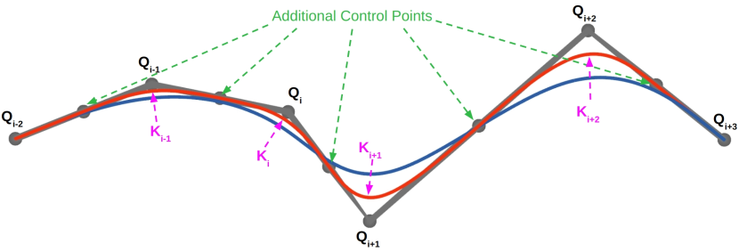
Figure 2: Clamped B-spline curve. This curve is made by adding control points between successive control points. The curvature $K_{i}$ ($u=0.5$) of the clamped B-spline curve (red) is bigger than the curvature $\kappa_{t}$ of the B-spline curve (blue) at time $t$.

III-D SV Estimation Method

SV for quadrotors require only fixed-radius discs for the safety of the entire trajectory because of their circular shape. However, such fixed-radius discs for the SV of AVs restrict the problem solution area (e.g., narrow corridor) because of the SV over-approximation, which requires a large radius disc ($\geq\textit{vehicle-length}/2$) to cover the rectangular body shapes of AVs. Therefore, both discrete- and continuous-time SV estimation methods, which involve discs with different radii, are used to avoid over-approximating the actual vehicle SV. Here, we summarize the discrete-time SV estimation method[8, 24] and introduce a new continuous-time SV estimation method.

III-D1 Discrete-Time SV Estimation Method

The vehicle has a rectangular body that can be covered with $\textsc{N}_{\textsc{DISC,O}}$ discs, and the discs have the same radius $\textsc{R}_{\textsc{DISC,O}}$, as shown in Fig. 3. The point $(x_{t},y_{t})$ is the same as point $\bm{p}_{t}$ of the B-spline curve at time $t$. The four vertices of the ego vehicle are $F_{L}=(x_{F_{L}},y_{F_{L}}),F_{R}=(x_{F_{R}},y_{F_{R}}),R_{R}=(x_{R_{R}},y_{R_{R}})$, and $R_{L}=(x_{R_{L}},y_{R_{L}})$:

$$x_{F_{L}}(t)=x(t)+(\textsc{L}_{\textsc{W}}+\textsc{L}_{\textsc{F}})\cdot\cos{\theta^{(1)}}(t)-0.5\textsc{L}_{\textsc{B}}\cdot\sin{\theta^{(1)}}(t),$$ (5)

$$y_{F_{L}}(t)=y(t)+(\textsc{L}_{\textsc{W}}+\textsc{L}_{\textsc{F}})\cdot\sin{\theta^{(1)}}(t)+0.5\textsc{L}_{\textsc{B}}\cdot\cos{\theta^{(1)}}(t),$$

$$x_{F_{R}}(t)=x(t)+(\textsc{L}_{\textsc{W}}+\textsc{L}_{\textsc{F}})\cdot\cos{\theta^{(1)}}(t)+0.5\textsc{L}_{\textsc{B}}\cdot\sin{\theta^{(1)}}(t),$$

$$y_{F_{R}}(t)=y(t)+(\textsc{L}_{\textsc{W}}+\textsc{L}_{\textsc{F}})\cdot\sin{\theta^{(1)}}(t)-0.5\textsc{L}_{\textsc{B}}\cdot\cos{\theta^{(1)}}(t),$$

$$x_{R_{R}}(t)=x(t)-\textsc{L}_{\textsc{R}}\cdot\cos{\theta^{(1)}}(t)+0.5\textsc{L}_{\textsc{B}}\cdot\sin{\theta^{(1)}}(t),$$

$$y_{R_{R}}(t)=y(t)-\textsc{L}_{\textsc{R}}\cdot\sin{\theta^{(1)}}(t)-0.5\textsc{L}_{\textsc{B}}\cdot\cos{\theta^{(1)}}(t),$$

$$x_{R_{L}}(t)=x(t)-\textsc{L}_{\textsc{R}}\cdot\cos{\theta^{(1)}}(t)-0.5\textsc{L}_{\textsc{B}}\cdot\sin{\theta^{(1)}}(t),$$

$$y_{R_{L}}(t)=y(t)-\textsc{L}_{\textsc{R}}\cdot\sin{\theta^{(1)}}(t)+0.5\textsc{L}_{\textsc{B}}\cdot\cos{\theta^{(1)}}(t).$$

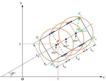
Figure 3: Example of discrete-time SV estimation with three discs.

The disc radius is calculated as

$$\textsc{R}_{\textsc{DISC,O}}=\sqrt{(\frac{\textsc{L}_{\textsc{R}}+\textsc{L}_{\textsc{W}}+\textsc{L}_{\textsc{F}}}{2\textsc{N}_{\textsc{DISC,O}}})^{2}+(\frac{\textsc{L}_{\textsc{B}}}{2})^{2}},$$ (6)

and the center points of the discs $disc^{ok}=(x^{disc,ok},y^{disc,ok})$ are defined as

$$x^{disc,ok}(t) =x(t)+\Bigg{(}\frac{2k-1}{2\textsc{N}_{\textsc{DISC,O}}}\cdot(\textsc{L}_{\textsc{R}}+\textsc{L}_{\textsc{W}}+\textsc{L}_{\textsc{F}})-\textsc{L}_{\textsc{R}}\Bigg{)}$$ (7)

$$\cdot\cos{\theta^{(1)}}(t),$$

$$y^{disc,ok}(t) =y(t)+\Bigg{(}\frac{2k-1}{2\textsc{N}_{\textsc{DISC,O}}}\cdot(\textsc{L}_{\textsc{R}}+\textsc{L}_{\textsc{W}}+\textsc{L}_{\textsc{F}})-\textsc{L}_{\textsc{R}}\Bigg{)}$$

$$\cdot\sin{\theta^{(1)}}(t),$$

$$k\in\{1,\ldots,\textsc{N}_{\textsc{DISC,O}}\},t\in[t_{p_{b}},t_{M-p_{b}}].$$

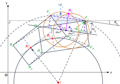
Figure 4: Example of continuous-time SV estimation (CW).

III-D2 Continuous-Time SV Estimation Method

The discrete-time SV estimation method is formulated for a discretely sampled trajectory. However, the continuous execution of a trajectory may involve a collision between time steps. Therefore, an estimation method of the vehicle body continuous-time SV [22] is introduced. Our SV estimation method is a disc-type estimation approach that can minimize SV over-approximation using minimum-radius discs rather than convex polygons [22, 23, 24], which lead to redundant regions at curves.

To find the minimum disc radius, we focus on the outer vertices comprising the maximum SV between two consecutive time knots $(t_{m},t_{m+1})$. The outer vertices are defined as $v$ at $t_{m}$ and $v^{{}^{\prime}}$ at $t_{m+1}$. The SV formed by the inner vertices is excluded because it can be covered by the discrete-time SV estimation and the circle collision avoidance constraint, as shown in Fig. 7. The outer vertices are the two left vertices ($F_{L}$ and $R_{L}$ in Fig. 4) of the vehicle when it turns clockwise (CW) and the two right vertices ($F_{R}$ and $R_{R}$ in Fig. 4) of the vehicle when it turns counter-clockwise (CCW). The SV is estimated using discs with the minimum radius by following the steps.

First, outer vertices pairs $(v,v^{{}^{\prime}})$ at two consecutive time knots of the B-spline curve are identified ($(F_{L}$, ${F_{L}}^{{}^{\prime}})$ and $(R_{L}$, ${R_{L}}^{{}^{\prime}})$ in Fig. 4). Then, outside vertices, which are outside the vehicle box at different time knots, among the outer vertices pairs are defined as a set $\mathbf{V}$ ($(F_{L},F_{L}^{{}^{\prime}})$ in Fig. 4). The inside outer vertices pairs ($(R_{L}$, ${R_{L}}^{{}^{\prime}})$ in Fig. 4) are excluded because of the same reason as the inner vertices.

Second, the $N_{DISC,V}$ discs for covering an SV are obtained as $\lceil\overline{vv^{{}^{\prime}}}/\textsc{R}_{\textsc{DISC,O}}\rceil$, and a new point $A_{v}=(x_{A_{v}},y_{A_{v}})$ is defined as

$$x_{A_{v}}(t) =\frac{x_{v}+x_{v^{{}^{\prime}}}}{2}+H_{v}(t)\cdot\cos{\theta_{A}(t)},$$ (8)

$$y_{A_{v}}(t) =\frac{y_{v}+y_{v^{{}^{\prime}}}}{2}+H_{v}(t)\cdot\sin{\theta_{A}(t)},$$

where

$$\theta_{A}(t)=\left\{\begin{array}[]{lr}\theta_{v}(t)-\frac{\pi}{2}&(\textsc{CW})\\ \theta_{v}(t)+\frac{\pi}{2}&(\textsc{CCW})\end{array}\right.,$$ (9)

$H_{v}(t)=\frac{\textsc{L}_{\textsc{B}}}{2}\cdot|\cos({\theta^{(1)}_{t_{m+1}}-\theta_{v}(t)})|$, $\theta_{v}$ is a new angle of the line segment $\overline{vv^{{}^{\prime}}}$, and $(v,v^{{}^{\prime}})\in\mathbf{V}$. The center points of the new discs $disc^{vk}=(x^{disc,vk},y^{disc,vk})$ are obtained as

$$x^{disc,vk}(t) =x_{A_{v}}(t)+\Bigg{(}\frac{2k-1}{2N_{DISC,V}}\cdot\overline{vv^{{}^{\prime}}}-\frac{\overline{vv^{{}^{\prime}}}}{2}\Bigg{)}\cdot\cos{\theta}_{v}(t),$$ (10)

$$y^{disc,vk}(t) =y_{A_{v}}(t)+\Bigg{(}\frac{2k-1}{2N_{DISC,V}}\cdot\overline{vv^{{}^{\prime}}}-\frac{\overline{vv^{{}^{\prime}}}}{2}\Bigg{)}\cdot\sin{\theta}_{v}(t),$$

$$k\in\{1,\ldots,N_{DISC,V}\}.$$

The disc radius is initially reduced as $\widehat{R}_{DISC,V}=min(\overline{A_{v}v},\textsc{R}_{\textsc{DISC,O}})$ to prevent SV over-approximation ( $\overline{A_{v}v}$ is the minimum disc radius needed to cover the SV with one disc). Furthermore, using more than one disc can reduce over-approximation by covering the SV with a smaller-radius disc. To fully cover the SV ($\downslice{F_{L}}$ in Fig. 4), the minimum distance from $A_{F_{L}}$ to disc $B_{F_{L}}$ (namely, $\overline{A_{v}B_{v}}$) has to be longer than the maximum distance from $A_{F_{L}}$ to the intercepted arc (namely, $\overline{Iv^{{}^{\prime}}}-\overline{IA_{v}}$) where $\overline{A_{v}B_{v}}=\sqrt{(\widehat{R}_{DISC,V})^{2}-(\overline{A_{v}C_{v}})^{2}}$. Here, $C_{v}$ is the center point of the disc $disc^{vk}$ at $k=\lceil N_{DISC,V}/2\rceil$ and is thus the closest point of the disc to the point $A_{v}$. Finally, the disc radius $R_{DISC,V}$ is obtained as

$$R_{DISC,V}=$$ (11)

$$\left\{\begin{array}[]{lr}\widehat{R}_{DISC,V}&(\overline{A_{v}B_{v}}\geq\overline{Iv^{{}^{\prime}}}-\overline{IA_{v}})\\ \sqrt{(\overline{Iv^{{}^{\prime}}}-\overline{IA_{v}})^{2}+(\overline{A_{v}C_{v}})^{2}}&(\overline{A_{v}B_{v}}<\overline{Iv^{{}^{\prime}}}-\overline{IA_{v}})\end{array}\right.,$$

where $I$ is the instantaneous center of rotation of the ego vehicle. The continuous-time SV estimation is formulated using the minimum-radius $R_{DISC,V}$ discs (we call C-SV discs) that can cover the SV $\downslice{F_{L}}$. Thus, it can be used for the optimization algorithm of safe and efficient trajectories.

IV B-spline Trajectory Optimization

The proposed B-spline-based trajectory optimization approach has two optimization stages based on EGO-Planner [9]. The first stage called rebound optimization, iteratively finds a smooth and collision-free trajectory with two collision avoidance constraints: circle and kinematics collision avoidance constraints. The circle collision avoidance constraint is collision checking with one disc, which has radius $\textsc{R}_{\textsc{CIRCLE}}$ as shown in Fig. 6(a), and the kinematics collision avoidance constraints are collision checking with the discrete- and continuous-time SV estimation methods in Section III-D on the optimized trajectory. The second optimization stage, called trajectory refinement, ensures that the optimized trajectory from the first stage is bounded by the kinodynamic feasibility constraints (velocity, acceleration, and curvature) if it violates the kinodynamic feasibility constraints.

IV-A Problem Formulation

The collision-free trajectory $\Gamma$ is parameterized to the reference uniform B-spline curve $\bm{\Phi}^{ref}$ with the same time interval $\Delta t$. Because both the initial and final state boundary conditions for the B-spline $\{\mathbf{p}_{t_{p_{b}}},\mathbf{v}_{t_{p_{b}}},\mathbf{a}_{t_{p_{b}}},\theta^{(1)}_{t_{p_{b}}},\mathbf{p}_{t_{M-p_{b}}},\mathbf{v}_{t_{M-p_{b}}},\mathbf{a}_{t_{M-p_{b}}},\theta^{(1)}_{t_{M-p_{b}}}\}$ are determined, control points $\{\mathbf{Q}_{p_{b}},\mathbf{Q}_{p_{b}+1},\ldots,\mathbf{Q}_{N_{c}-p_{b}}\}$ without the initial and final $p_{b}$ control points are used as the control variables for optimization.

The rebound optimization cost function $J$ is formulated as

$$\min_{\bm{Q}}J=\lambda_{sm}J_{sm}+\lambda_{cl}J_{cl}+\lambda_{fl}J_{fl},$$ (12)

where $J_{sm}$, $J_{cl}$, and $J_{fl}$ are smoothness, collision, and flattening penalties respectively, and $\lambda_{sm}$, $\lambda_{cl}$, and $\lambda_{fl}$ are their corresponding weights.

IV-A1 Smoothness Penalty

The smoothness penalty cost, which minimizes the high-order derivatives and curvature of the whole trajectory, is defined as

$$J_{sm}=\sum_{i=0}^{N_{c}-2}\Bigl{(}\frac{{\|\mathbf{A}_{i}\|}}{s_{\text{A}}}\Bigl{)}^{2}+\sum_{i=0}^{N_{c}-3}\Bigl{(}\frac{{\|\mathbf{J}_{i}\|}}{s_{\text{J}}}\Bigl{)}^{2}+\sum_{i=1}^{N_{c}-1}\Bigl{(}\frac{{K_{i}}}{\kappa_{\text{max}}}\Bigl{)}^{2},$$ (13)

where $s_{\text{A}}$ and $s_{\text{J}}$ are scale parameters for the acceleration and jerk, respectively, and $\kappa_{\text{max}}$ is the maximum parameter of curvature.

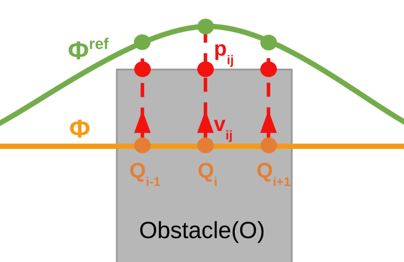
(a) Collision Obstacle

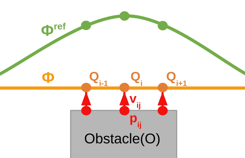
(b) Close Obstacle

Figure 5: Obstacle penalty: (a) collision obstacle, (b) close obstacle. For the collision obstacle trajectory $\mathbf{\Phi}$, the anchor point $\mathbf{p}_{ij}$ is the closest point at the obstacle surface from the line between the corresponding control points $\mathbf{Q}_{i}$ and $\mathbf{Q}^{ref}_{i}$, and the direction vector $\mathbf{v}_{ij}$ is a unit vector pointing toward $\mathbf{p}_{ij}$ from $\mathbf{Q}_{i}$. For the close-obstacle trajectory $\mathbf{\Phi}$, which is within a safe clearance $s_{f}$, the anchor point $\mathbf{p}_{ij}$ is the closest point from the corresponding control point $\mathbf{Q}_{i}$, and the direction vector $\mathbf{v}_{ij}$ is pointing toward $\mathbf{Q}_{i}$ from $\mathbf{p}_{ij}$.

IV-A2 Collision Penalty

EGO-Planner [9] generates $\{\mathbf{p}_{ij},\mathbf{v}_{ij}\}$, where $\mathbf{p}_{ij}$ is an anchor point and $\mathbf{v}_{ij}$ is a repulsive direction vector, for a collision segment of a trajectory in an iteration. However, unlike in EGO-Planner, an additional collision penalty from close obstacles is required because the reference trajectory $\bm{\Phi}^{ref}$ initially does not collide with obstacles. Therefore, the close-obstacle penalty is formulated, as shown in Fig. 5. It pushes the path away from nearby obstacles, thus reducing the collision risk. In addition, it works with the IPF method to find a collision-free path. The collision penalty is

$$J_{cl}=\sum_{i=p_{b}}^{N_{c}-p_{b}}\sum_{j=1}^{N_{p}}j_{cl}(i,j),$$ (14)

where $j_{cl}(i,j)$ is the cost function [9] and $N_{p}$ is the number of $\{\mathbf{p}_{ij},\mathbf{v}_{ij}\}$ pairs.

IV-A3 Flattening Penalty

The flattening penalty can locally flatten a path around vehicle collision points to find a collision-free path by reducing the SV. It is formulated as

$$J_{fl}=\sum_{i\in\mathbf{\Omega}^{fl}}w_{i}^{fl}\Bigl{(}\frac{{K_{i}}}{\kappa_{\text{max}}}\Bigl{)}^{2},$$ (15)

where $\mathbf{\Omega}^{fl}$ is a flattening index set (Section IV-B) and $w_{i}^{fl}$ is a local flattening weight at the control point $\mathbf{Q}_{i}$. It locally reduces the curvature $K_{i}$ by increasing the flattening weight.

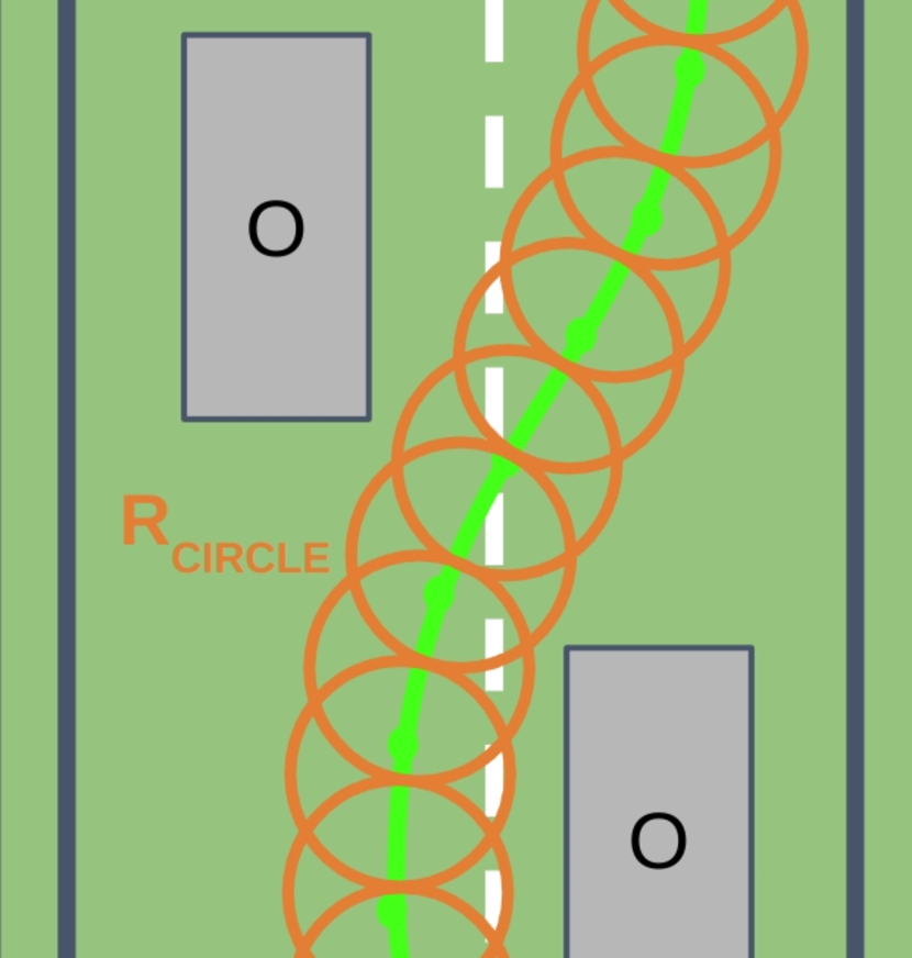
(a)

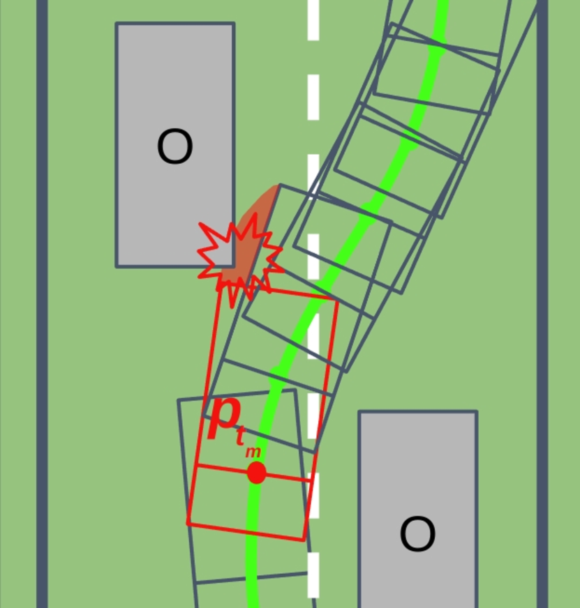
(b)

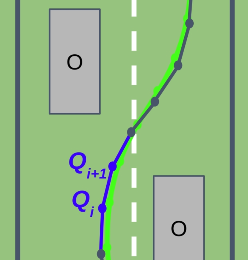
(c)

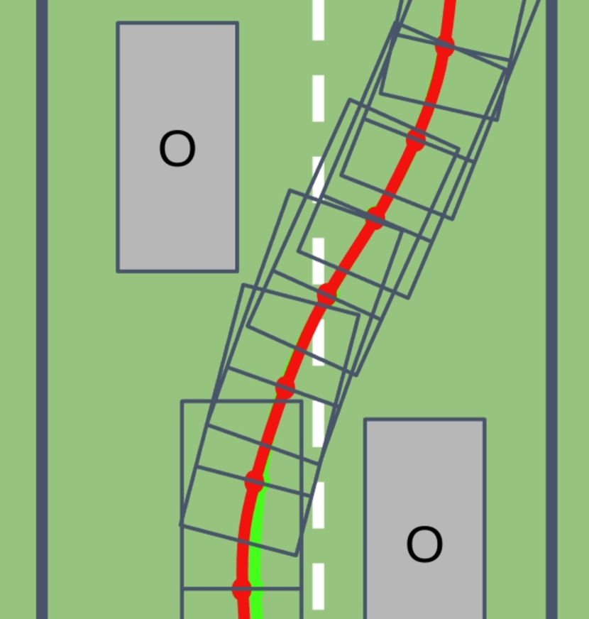
(d)

Figure 6: IPF process. (a) No collision occurs along the optimized trajectory, which has a disc radius $\textsc{R}_{\textsc{CIRCLE}}$. (b) The optimized trajectory has a collision, as determined via kinematics collision avoidance constraints, at a time knot $t_{m}$. (c) The flattening control points $\mathbf{Q}_{i},i\in\mathbf{\Omega}^{fl}$ are found. (d) A collision-free path is found via IPF.

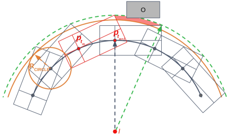
Figure 7: Circle collision avoidance constraint with a disc radius $\textsc{R}_{\textsc{CIRCLE}}$. This constraint (orange arc) cannot fully cover the kinematics collision avoidance constraints (green arc). An obstacle (gray) is placed between the circle and the kinematics collision avoidance constraints.

Algorithm 1 Rebound Optimization with IPF

Input: Collision-free trajectory $\bm{\Gamma}$
Output: Optimized trajectory $\bm{\Phi}^{opt}$

1:$\bm{Q}\leftarrow\textsc{P{arameterize}T{o}B{spline}}(\bm{\Gamma})$

2:$\bm{C}\leftarrow\textsc{G{en}C{ollision}V{ector}}(\bm{Q})$

3:while $iter\leq\text{iter}_{\text{max}}$ do

4:     $\bm{\Phi}^{opt}\leftarrow\textsc{U{niform}B{spline}}(\bm{Q})$

5:     if $\textsc{{is}C{ircle}C{ollision}}(\bm{\Phi}^{opt})$ then

6:         $\bm{C}\leftarrow\textsc{G{en}C{ollision}V{ector}}(\bm{Q})$

7:     else if $\textsc{{is}K{inematics}C{ollision}}(\bm{\Phi}^{opt})$ then

8:         $\mathbf{\Omega}^{fl}\leftarrow\textsc{F{ind}F{lattening}I{ndex}S{et}}(\bm{\Phi}^{opt})$

9:         $w_{i}^{fl}\leftarrow\gamma^{fl}\cdot w_{i}^{fl},i\in\mathbf{\Omega}^{fl}$

10:     else

11:         return true

12:     end if

13:     $(J,\bm{G})\leftarrow\textsc{E{valuate}P{enalty}}(\bm{Q})$

14:     $\bm{Q}\leftarrow\textsc{T{rajectory}O{ptimize}}(J,\bm{G})$

15:     $iter\leftarrow iter+1$

16:end while

IV-B IPF

The collision penalty of EGO-Planner is formulated to push control points away from nearby obstacles instead of the trajectory of the B-spline curve. Because the B-spline curve binds the path and control points together [34], it can find the collision-free path using the collision penalty. Furthermore, the use of the collision penalty is enough for finding collision-free path for quadrotors because they are covered by the same disc-radius constraint (with small over-approximation). However, large disc-radius constraint ($\textsc{R}_{\textsc{DISC}}\geq\textit{vehicle-length}/2$) is needed to cover an AV body, which is rectangular; otherwise, some of the vehicle body will not be covered in a curve path. As shown in Fig. 7, a circle collision avoidance constraint with a small disc radius $\textsc{R}_{\textsc{CIRCLE}}$ cannot cover the vehicle’s SV. The proposed IPF method can reduce the size of the uncovered region by reducing the curvatures around the collision path. The shrunk region can be covered by the circle collision avoidance constraint because the collision penalty from EGO-Planner, which is designed to be used for circular vehicles, ensures that the trajectory is free of collisions.

The collision time $t_{c}$ lies between knot vectors $[t_{m},t_{m+1})$. A collision index set of the knot vectors that can be found by the kinematics collision avoidance constraints is defined as

$$\mathbf{\Omega}^{coll} =\{m\in H\mid dist(f_{disc,j}(\mathbf{\Phi}(t_{m})))\leq R_{disc,j}\},$$ (16)

$$H =\{p_{b},p_{b}+1,\ldots,M-p_{b}\},$$

where $j\in\{O,\mathbf{V}\}$; $\mathbf{V}$ is the outside pair set from the continuous-time collision avoidance constraint, $f_{disc,O}$ and $f_{disc,v}$ are disc point functions of (7) and (10), respectively; and $dist(\bm{p}_{t})$ is a function that determines the distance from $\bm{p}_{t}$ to the closest obstacle. KD-tree [35] is used for the $dist(\bm{p}_{t})$ function in this work. The curvature of the B-spline curve between the knot vectors $[t_{m},t_{m+1})$ is always smaller than the curvature $max\{|K_{m-p_{b}+1}|,|K_{m-p_{b}+2}|\}$ of the clamped B-spline curve. Therefore, the collision time index set is extended to a flattening index set as

$$\mathbf{\Omega}^{fl}=\{m-p_{b}+1,m-p_{b}+2\mid m\in\mathbf{\Omega}^{coll}\}.$$ (17)

The IPF process ensures that the trajectory is free of collisions by iteratively increasing the flattening weights, as shown in Fig. 6. The IPF algorithm is presented as Algorithm 1. Here, we set three terminal conditions for TrajectoryOptimize(): when the optimization gradient is lower than $\epsilon_{g}$, when the amount of the cost change is lower than $\epsilon_{c}$, or at every $\alpha$ iteration of the trajectory optimization for early exit. If isCircleCollision(), which is the collision-checking function of the circle collision avoidance constraint, is true, then collision vectors are generated. If isKinematicsCollision(), which is the collision-checking function of the kinematics collision avoidance constraints (Section III-D), is true, then the flattening weight $w^{fl}_{i}$ is iteratively increased such that the local flattening weight ratio $\gamma^{fl}>1$ and $i\in\mathbf{\Omega}^{fl}$.

Algorithm 2 Refinement Optimization

Input: Re-allocated control points $\bm{Q}$
Output: Optimized trajectory $\bm{\Phi}^{opt}$

1:while $iter\leq\text{iter}_{\text{max}}$ do

2:     $\bm{\Phi}^{opt}\leftarrow\textsc{U{niform}B{spline}}(\bm{Q})$

3:     if $\textsc{{is}C{ollision}}(\bm{\Phi}^{opt})$ then

4:         $\lambda_{ft}\leftarrow\gamma^{ft}\cdot\lambda_{ft}$

5:     else if $\textsc{{is}F{easible}}(\bm{\Phi}^{opt})$ then

6:         return true

7:     end if

8:     $(J,\bm{G})\leftarrow\textsc{E{valuate}P{enalty}}(\bm{Q})$

9:     $\bm{Q}\leftarrow\textsc{T{rajectory}O{ptimize}}(J,\bm{G})$

10:     $iter\leftarrow iter+1$

11:end while

Algorithm 3 B-spline Trajectory Optimization

Input: Collision-free trajectory $\bm{\Gamma}$
Output: Optimized trajectory $\bm{\Phi}^{opt}$

1:$\bm{\Phi}^{opt}\leftarrow\textsc{R{ebound}O{ptimization}W{ith}IPF}(\bm{\Gamma})$

2:if not $\textsc{{is}F{easible}}(\bm{\Phi}^{opt})$ then

3:     $\bm{\Phi}\leftarrow\textsc{R{e}A{llocation}T{ime}}(\bm{\Phi}^{opt})$

4:     $\bm{Q}\leftarrow\textsc{G{et}C{ontrol}P{oints}}(\bm{\Phi})$

5:     $\bm{\Phi}^{opt}\leftarrow\textsc{R{efinement}O{ptimization}}(\bm{Q})$

6:end if

7:return $\bm{\Phi}^{opt}$

IV-C Trajectory Refinement

The initial time allocation of the initial trajectory is inaccurate because the trajectory can be largely modified by obstacles. This modification can make the trajectory violate the feasibility constraints, such as velocity and acceleration. Therefore, researchers [36] and [9] relax the violation criterion through time reallocation by lengthening the knot spans with the maximum exceeding ratio of the derivative limits to the axes of all knot spans. The limits exceeding ratio [36, 9] is $r_{e}=max\{1,|\mathbf{V}_{r}/v_{\text{max}}|,\sqrt[2]{|\mathbf{A}_{r}/a_{\text{max}}|},\sqrt[3]{|\mathbf{J}_{r}/j_{\text{max}}|}\}$, where $r\in\{x,y,z\}$ axis. Therefore, the limits exceeding ratio relaxes the velocity as $\mathbf{V}_{r}^{{}^{\prime}}=\mathbf{V}_{r}/r_{e}$ and the acceleration as $\mathbf{A}_{r}^{{}^{\prime}}=\mathbf{A}_{r}/r_{e}$. Because the L2 norm is $\|\mathbf{x}\|=\sqrt{x_{1}^{2}+x_{2}^{2}}$, the velocity and acceleration norms can be also relaxed as $\|\mathbf{V}^{{}^{\prime}}\|=\|\mathbf{V}\|/r_{e}$ and $\|\mathbf{A}^{{}^{\prime}}\|=\|\mathbf{A}\|/r_{e}$, respectively. Therefore, the limits exceeding ratio from the longitudinal and lateral velocity and acceleration is

$$r_{e}=max\{1,v_{t}^{s}/v_{m}^{s},\sqrt{a_{t}^{s}/a_{m}^{s}},\sqrt{a_{t}^{d}/a_{m}^{d}}\},$$ (18)

where $t\in[t_{p_{b}},t_{M-p_{b}}]$, and the subscript $m$ denotes the maximum if the derivative is greater than or equal to zero and the minimum if the derivative is less than zero.

The optimization cost function $J^{{}^{\prime}}$ for refinement is reformulated as

$$\min_{\bm{Q}}J^{{}^{\prime}}=\lambda_{sm}J_{sm}+\lambda_{ft}J_{ft}+\lambda_{fs}J_{fs},$$ (19)

where $J_{ft}$ and $J_{fs}$ are fitness and feasibility penalties, respectively, and $\lambda_{ft}$ and $\lambda_{fs}$ are their corresponding weights.

IV-C1 Fitness Penalty

Instead of the collision penalty, the fitness penalty ensures that the optimized trajectory is free of collisions because this refinement stage does not make a large modification in the trajectory shape after rebound optimization. It pulls the optimized trajectory toward the collision-free trajectory, which is from the rebound optimization, using anisotropic displacements between the two trajectories. We use the fitness penalty function $j_{ft}$ [9], which is calculated as

$$J_{ft}=\sum_{i=p_{b}}^{N_{c}-p_{b}}j_{ft}(i).$$ (20)

The fitness weight $\lambda_{ft}$ increases by the fitness weight ratio $\gamma^{ft}$ if the path has a collision.

IV-C2 Kinodynamic Feasibility Penalty

A kinodynamic feasibility penalty enables the AV to meet the kinodynamic feasibility constraints by confining the derivatives and curvature of the trajectory within their limitations. The feasibility penalty cost function is formulated as

$$J_{fs}= \int_{t_{p_{b}}}^{t_{M-p_{b}}}j_{fs}(v_{t}^{s})dt+\int_{t_{p_{b}}}^{t_{M-p_{b}}}j_{fs}(a_{t}^{s})dt$$ (21)

$$+\int_{t_{p_{b}}}^{t_{M-p_{b}}}j_{fs}(a_{t}^{d})dt+\sum_{i={1}}^{N_{c}-1}j_{fs}(K_{i}),$$

where $j_{fs}$ is a twice continuously differentiable function similar to the feasibility penalty of [9]. We use the Gauss–Legendre n-point quadrature formula [37] to calculate the integral in (21).

$$j_{fs}(c)=\left\{\begin{array}[]{lr}a_{1}(c/c_{m})^{2}+b_{1}(c/c_{m})+c_{1}&(c/c_{m}\geq 1)\\ (c/c_{m}-\lambda)^{3}&(\lambda<c/c_{m}<1)\\ 0&(-\lambda\leq c/c_{m}\leq\lambda)\\ (\lambda-c/c_{m})^{3}&(-1<c/c_{m}<-\lambda)\\ a_{2}(c/c_{m})^{2}+b_{2}(c/c_{m})+c_{2}&(c/c_{m}\leq-1)\end{array}\right.,$$ (22)

where $a_{1},b_{1},c_{1},a_{2},b_{2}$, and $c_{2}$ are selected for second-order continuity; $0<\lambda\leq 1$ is an elastic coefficient; and the subscript $m$ denotes the maximum if $c\geq 0$ and the minimum if $c<0$. The refinement optimization algorithm, shown as in Algorithm 2, starts with the reallocated control points from the trajectory optimized during rebound optimization using IPF if the isFeasible() function is false. This function checks whether the kinodynamic feasibility constraints (velocity, acceleration, and curvature) are violated. If isCollision(), which is true if either isCircleCollision() or isKinematicsCollision() is true, is true, then the fitness weight is iteratively increased by $\gamma^{ft}$ to make a collision-free trajectory using the fitness penalty. The terminal conditions for TrajectoryOptimize() are from Algorithm 1. The entire B-spline trajectory optimization algorithm is presented as Algorithm 3.

V Evaluations

TABLE I: Simulation parameter settings

Parameter	Description and unit	Value
$p_{b}$	Degree of B-spline curve	3
$\textsc{N}_{\textsc{DISC}}$	Number of discs (s)	5
$\textsc{L}_{\textsc{F}}$	Front hang length of the ego vehicle (m)	1.015
$\textsc{L}_{\textsc{R}}$	Rear hang length of the ego vehicle (m)	1.015
$\textsc{L}_{\textsc{W}}$	Wheelbase of the ego vehicle (m)	2.87
$\textsc{L}_{\textsc{B}}$	Width of the ego vehicle (m)	1.86
$v^{s}_{\text{max}},v^{s}_{\text{min}}$	Max & Min longitudinal velocity ($m/s$)	5.55, 0.00
$a^{s}_{\text{max}},a^{s}_{\text{min}}$	Max & Min longitudinal acceleration ($m/s^{2}$)	4.0, -4.0
$a^{d}_{\text{max}},a^{d}_{\text{min}}$	Max & Min lateral acceleration ($m/s^{2}$)	2.0, -2.0
$\kappa_{\text{max}},\kappa_{\text{min}}$	Max & Min curvature ($m^{-1}$)	0.2, -0.2
$\Delta t$	Time interval	$\text{L}_{\text{W}}/2v^{s}_{\text{max}}$
$\textsc{R}_{\textsc{CIRCLE}}$	Circle disc radius (m)	$\textsc{R}_{\textsc{DISC}}$
$s_{f}$	Safe clearance (m)	$2\textsc{R}_{\textsc{DISC}}$
$\lambda$	Elastic coefficient	0.8
$\text{iter}_{\text{max}}$	Max rebound & refinement iteration	10
$\epsilon_{g},\epsilon_{c}$	Gradient & Cost epsilon	1e-2, 1e-5
$\alpha$	early exit iteration number	100
$s_{\text{A}},s_{\text{J}}$	scale parameter for acceleration and jerk	3.0, 5.0
$\lambda_{sm}$	Weight for smoothness penalty	1.0
$\lambda_{cl}$	Weight for collision penalty	1.0
$\lambda_{fl}$	Weight for flattening penalty	1.0
$\lambda_{ft}$	Weight for fitness penalty	2.0
$\lambda_{fs}$	Weight for feasibility penalty	5.0
$w_{i}^{fl}$	Local flattening weight	1.0
$\gamma^{fl}$	Local flattening weight ratio	10.0
$\gamma^{ft}$	Fitness weight ratio	2.0

The effectiveness of the SV estimation method, IPF, and kinodynamic feasibility constraints and the tracking performance, efficiency, and robustness of the proposed algorithm were evaluated. The results demonstrate that our proposal outperformed two SOTA trajectory optimization algorithms [2, 8] in various environments. Path-velocity decoupled/coupled trajectory optimization algorithms, which are designed for car-like vehicles, were utilized as baselines to show the superiority of the proposed method over both algorithm types. A video of the experiments is available at https://youtu.be/7bhxfuhAqos.

V-A Simulation Setup

All simulation experiments were conducted on a desktop with a Ryzen 7 3800x CPU, which runs at 3.9GHz by default. We simulated experiments using the open-source simulator CARLA [38]. All parameter settings are listed in Table I. A solver, which enables fast restarting, was required because our problem needs repeated stopping, generation of new costs for obstacles, and restarting. According to the experiment results of [9], the L-BFGS method, which is capable of fast restarting, outperforms other quasi-Newton methods, such as the Barzilai–Borwein [39] and truncated Newton [40] method. Therefore, the L-BFGS solver was used in this experiment with Lewis–Overton line search [41] for non-convex optimization.

For a reference trajectory initially satisfying terminal constraints mentioned in Section III-A, the hybrid $\text{A}^{*}$ [42] algorithm was used to generate a kinematically feasible reference path and a trapezoidal velocity profile [10, 36] for an initial time allocation. The first baseline, called DL-IAPS [2], is a path-velocity decoupled planner solved using the QP solver OSQP [43]. The second baseline, called C-Planner [8], is a path-velocity coupled planner based on OCP that is solved using the NLP solver IPOPT [44]. The optimization time resolution $\delta t$ was set to $0.1s$ for DL-IAPS and $0.05s$ for C-Planner.

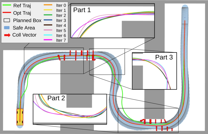
Figure 8: Trajectory optimization result with double narrow corridors and multiple curves. A reference trajectory is generated using the hybrid $\text{A}^{*}$ algorithm. The zoomed-in images show the optimizing path in each iteration. The planned boxes are generated at every $0.1s$.

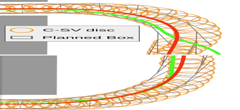
(a) C-SV discs

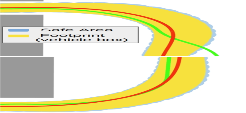
(b) Actual Vehicle SV

Figure 9: Evaluation of SV: (a) C-SV discs and planned vehicle boxes, (b) actual vehicle SV. In (a), the C-SV discs (orange) cover the planned vehicle boxes (gray boxes) at every time interval $\Delta t$ around the maximum curvature ($\approx\kappa_{\text{max}}$) of the path. The outside discs and inside discs are generated using the outside pairs $\{F_{L},F^{{}^{\prime}}_{L}\}$ and $\{R_{L},R^{{}^{\prime}}_{L}\}$, respectively. Some inside discs are not generated because the vertices of the pair are not outside of the vehicle box at different time steps. In (b), the safe area (blue) generated using the proposed SV estimation method can cover the footprint (yellow) of the vehicle box, which is the actual SV of the vehicle.

V-B SV Estimation Method

We evaluated whether the proposed SV estimation method can cover the actual vehicle SV between time steps. The evaluation environment (Fig. 8) had double narrow corridors and multiple curves, which required a sophisticated trajectory optimization algorithm with tight collision avoidance constraints. Fig. 9(a) shows that the SV discs from the continuous-time collision avoidance constraint fully covered the planned vehicle boxes at the maximum curvature of the path. The SV discs were generated between the outside outer vertices, and the number of SV discs adaptively increased to cover the bigger SV if the distance between two vertices increased. Fig. 9(b) illustrates that the estimated SV safely covered the actual vehicle SV and was slightly over-approximated relative to the actual vehicle SV.

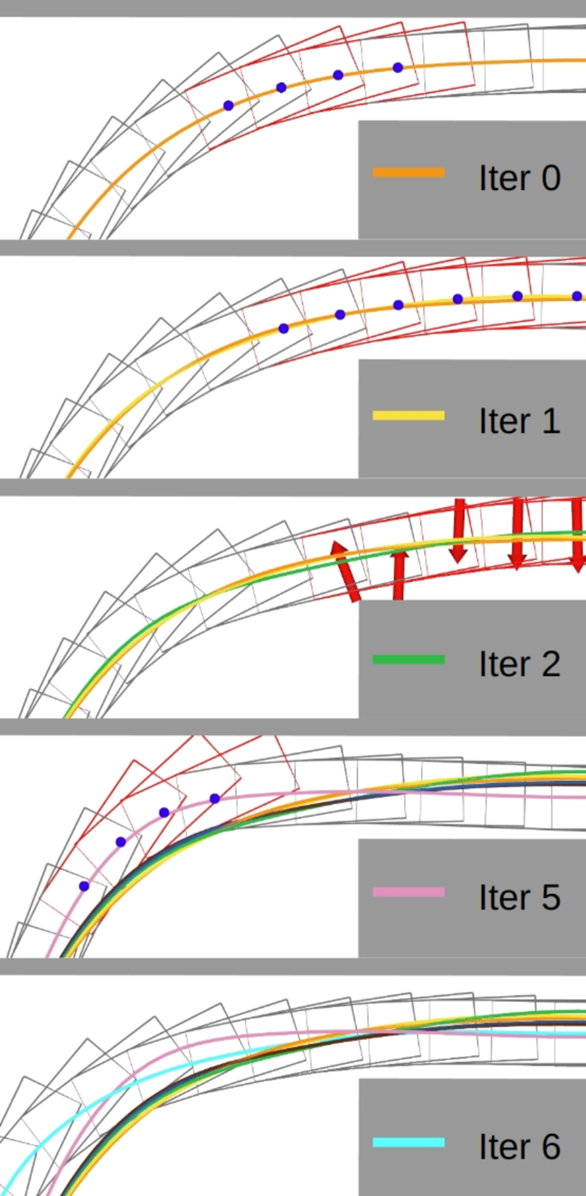
(a) Part 1

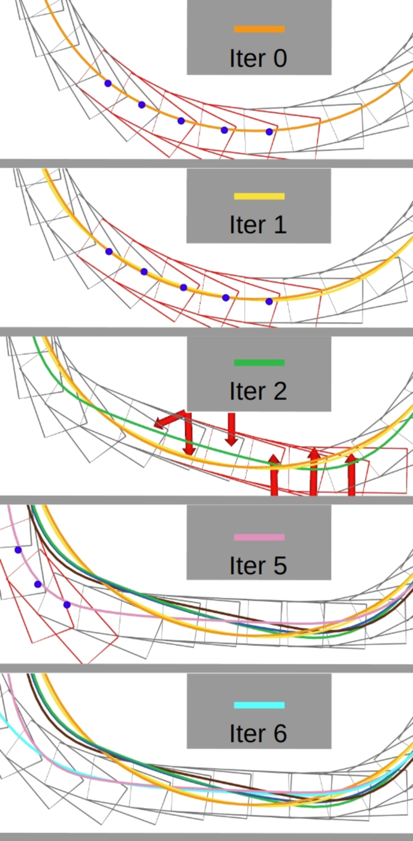
(b) Part 2

Figure 10: Iterations of rebound optimization with IPF: (a) part 1 in Fig. 8, (b) part 2 in Fig. 8. Planned collision-free vehicle boxes (gray boxes) and planned collision vehicle boxes (red boxes) are generated at every time interval $\Delta t$. The blue dots represent the flattening points $\mathbf{\Omega}^{flat}$, and the red arrows show the collision penalties from the nearby obstacles.

V-C IPF

The IPF method was evaluated in the same environment as the SV estimation method because the obstacle walls at the entrances of the narrow corridors made it difficult to generate a safe path. Fine changes had to be made in the path curvature before these entrances; otherwise, trajectory optimization would be rendered infeasible by the kinematics collision avoidance constraints. Therefore, we evaluated the IPF method by analyzing all iterations of the trajectory optimization algorithm, as shown in Fig. 8. The iterations at the entrances of the narrow corridors are enlarged in the figure (parts 1 and 2). Iterations 0-6 were from rebound optimization with IPF, and iteration 7 was from refinement optimization.

Each iteration of rebound optimization with IPF is illustrated in Fig. 10. Iterations 0, 1, and 5 in both parts generated flattening points due to vehicle kinematic collision, and no circle collision occurred. Then, the path of the next iterations 1, 2, and 6 was flattened near the vehicle collision points by increases in the flattening weights at the flattening points. However, this flattened path could collide with nearby obstacles, as shown in iteration 2. The collision penalty from the close obstacles pushed the path away from nearby obstacles. Consequently, a collision-free path was identified through the IPF method.

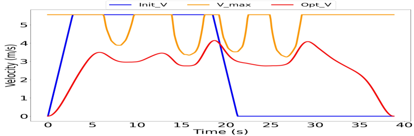
Figure 11: Velocity profile (red) of optimized trajectory with a maximum curvature velocity (yellow) obtained by $\sqrt{a^{d}_{\text{max}}/\kappa_{t}}$.

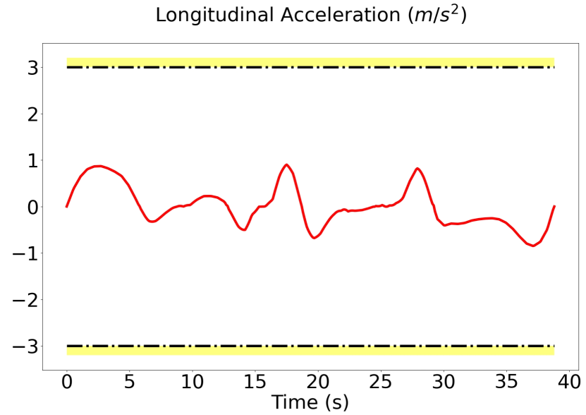
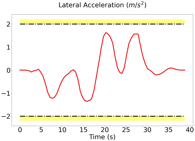
Figure 12: Longitudinal and lateral acceleration

V-D Trajectory Refinement

If the trajectory violates the kinodynamic feasibility constraints (velocity, acceleration, and curvature) after rebound optimization with IPF, then the trajectory refinement process makes it meet the constraints through time reallocation and refinement optimization. The maximum curvature of iteration 7, as shown in parts 1, 2, and 3 in Fig. 8, was decreased from $0.2595m^{-1}$ to $0.1909m^{-1}$ by the curvature constraint, and the other feasibility constraints were fulfilled. Fig. 11 shows that the proposed method met velocity and lateral acceleration constraints simultaneously. In addition, the longitudinal and lateral acceleration was bounded by the constraints, as shown in Fig. 12. Despite the challenging environment, which needed a long time horizon of $38.8s$ and multiple iterations, the computation times of rebound optimization with IPF and refinement optimization were $136ms$ and $93ms$, respectively.

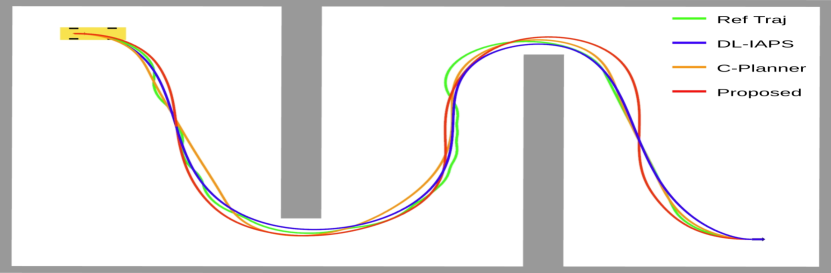
Figure 13: Evaluation of curvature constraint in the double-U-turn environment consisting of both a wide U-turn and a sharp U-turn. The reference trajectory is generated using the hybrid $\text{A}^{*}$ algorithm.

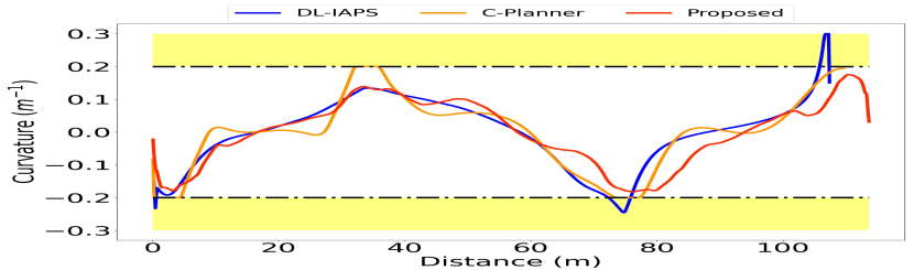
Figure 14: Comparison of curvature of optimized trajectories.

V-E Curvature Constraint

The curvature constraint of the proposed method was evaluated using the baselines in the double-U-turn environment shown in Fig. 13. We evaluated the curvature smoothness in the first (wide) U-turn part and the curvature constraint in the second (sharp) U-turn part.

The curvatures of the optimized trajectory from the proposed method and the baselines are compared in Fig. 14. C-Planner reached the maximum curvature in the first U-turn part, whereas DL-IAPS and the proposed method had smaller curvatures under the maximum curvature. Therefore, DL-IAPS and the proposed method generated smoother paths than C-Planner during the wide turn. These smoother paths could increase the maximum curvature velocity, as shown in Fig. 11, or lower the tracking error. Fig. 14 also shows that DL-IAPS violated the maximum curvature in the second U-turn part, whereas C-Planner and the proposed method did not exceed the curvature constraint. Therefore, the path from DL-IAPS could increase the tracking error. The curvatures in both U-turn parts show that the path from the proposed method was smoother, more tractable than the paths generated by the baselines. In addition, the computation times of the proposed method, DL-IAPS, and C-Planner were $93$, $3987$, and $3181ms$, respectively. The tracking performance of the compared methods was then analyzed in detail, as explained in the following Section V-F.

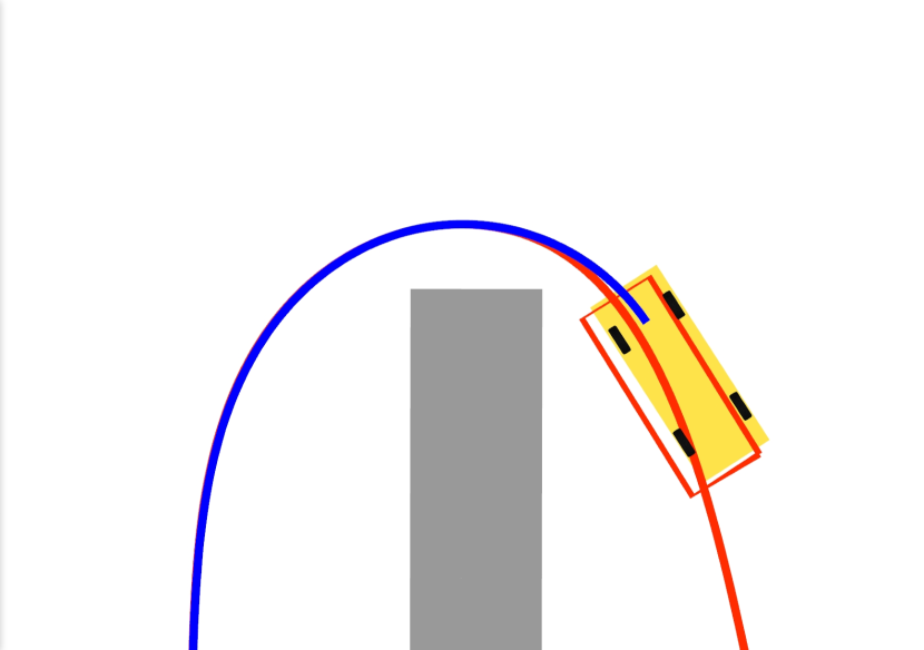
(a)

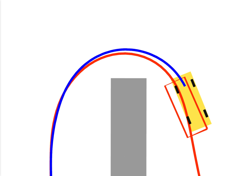
(b)

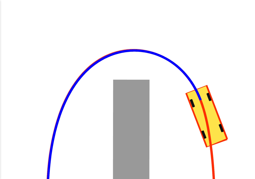
(c)

Figure 15: Comparison of tracking errors: (a) DL-IAPS, (b) C-Planner, (c) proposed method.

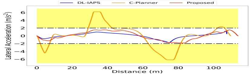
Figure 16: Comparison of lateral acceleration.

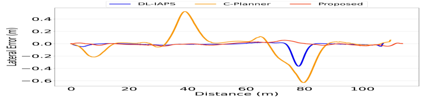
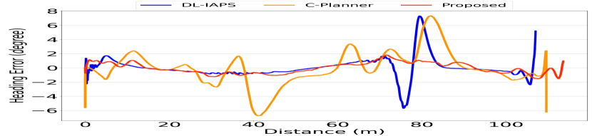
Figure 17: Comparison of lateral and heading errors.

V-F Tracking Performance

The tracking performance of the compared approaches was evaluated using their generated trajectories in the same environment (Fig. 13). We used a model predictive control (MPC)based controller to track the optimized trajectories. Fig. 15 demonstrates the displacement between the actual vehicle box and the planned vehicle box of the optimized trajectory in the second U-turn part. DL-IAPS and C-Planner had large displacements between the boxes and between the planned optimal trajectory and the footprint of the middle of the rear axle. The displacement of DL-IAPS was due to the violation of the maximum curvature, whereas that of C-Planner was due to the violation of the lateral acceleration constraint, as shown in Fig. 16, as lateral acceleration is not included in its algorithm. Conversely, the trajectory from the proposed method was tracked by the vehicle with little displacement.

For more details about the tracking error, Fig. 17 demonstrates the lateral and heading errors of the three methods throughout their trajectories. The baselines had absolute lateral errors of more than $0.3m$ and absolute heading errors of more than $7.0deg$, whereas the proposed algorithm had absolute lateral errors of less than $0.1m$ and absolute heading errors of less than $2.0deg$ at most. Thus, the proposed method was quantitatively superior in tracking performance.

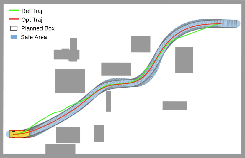
Figure 18: Random-obstacle test.

TABLE II: Computation times of proposed method

  Time (ms) Reference (Hybrid $\text{A}^{*}$) Optimization Steps Optimization Total Time Rebound Refinement   Min 103.98 17.85 10.79 28.65 Avg 309.54 33.60 26.24 59.84 Max 954.43 109.05 188.61 297.66  

  Method DL-IAPS [2] C-Planner [8] Proposed   Success^a Rate (%) 73.50 74.10 96.30 Success^b Rate (%) 99.60 74.10 99.40 Avg. Max. Abs Curvature ($m^{-1}$) 0.1958 0.1968 0.1497 Avg. Feas-Vio Score Long. Vel Long. Acc Lat. Acc Curvature 0.0000 0.0000 0.0000 0.0068 0.0000 0.0000 1.7281 0.0000 0.0000 0.0000 0.0000 0.0011 Avg. Planning Horizon (s) 24.96 14.75 17.18 Min. Comp Time (ms) 120.88 1385.50 28.65 Avg. Comp Time (ms) 1753.71 5988.27 59.84 Max. Comp Time(ms) 6256.03 30483.24 297.66   a The path is free of collision, and the violation of the kinodynamic feasibility constraints (velocity, acceleration, and curvature) is within 5%. Lateral acceleration is excluded from the success rate of C-Planner. b The conditions are the same as those of ${}^{\text{a}}$ but excluding the curvature constraint violation.

TABLE III: Comparison with baselines

V-G Random Obstacles

We evaluated the performance of the proposed method compared with the baselines in a random-obstacle environment. A maximum of 10 random-sized rectangular obstacles were randomly positioned between the fixed initial and final poses (position and heading angle), as shown in Fig. 18. The random test was conducted 1000 times for each algorithm.

The computation time of the proposed method is detailed in Table II. Aside from the reference computation time (that of hybrid $\text{A}^{*}$), the computation time of trajectory optimization is broken down into two stages (rebound and refinement) in the table. The average computation time in the refinement stage was $7.36ms$ faster than that in the rebound stage. However, the maximum time of the refinement stage was $79.56ms$ longer than the maximum time of the rebound stage. This was because the fitness penalty in the refinement stage made it difficult to lower curvature to meet the curvature constraint.

Table III shows our performance comparison of the proposed method and the baselines. We used two different success rates to determine the effect of the curvature constraint on the success of the method. The average maximum curvature was used to evaluate the smoothness of the paths generated by the algorithms. In addition, motivated by [45], we defined another metric called the Feasibility Violation Score to measure the extent of violation of the feasibility constraints. The Feasibility Violation Score is calculated as

Feasibility Violation Score $$=\frac{1}{T}\int_{0}^{T}max(0,|c|-c_{m})dt,$$ (23)

$$c\in\{v^{s},a^{s},a^{d},\kappa\},$$

where $c_{\text{m}}=min\{|c_{\text{min}}|,|c_{\text{max}}|\}$ and $T$ is the planning horizon, which is the duration to reach the goal.

Table III demonstrates the success rate of ${}^{\text{a}}$ (collision-free with violation of kinodynamic feasibility constraints of within $5\%$) of the proposed method was $96.3\%$, which was much higher than that of the baselines. The success rate of ${}^{\text{b}}$ (same condition as those of ${}^{\text{a}}$ but without curvature constraint violation) showed that the proposed method generated a highly feasible trajectory except for a curvature constraint violation. This happened when the optimized trajectory was tightly fit between obstacles, which required a large fitness weight and made the algorithm unable to minimize the curvature. The average maximum curvature showed that the proposed method could better minimize the smoothness of the trajectory for overall cases than the baselines. The average Feasibility Violation Scores indicated that DL-IAPS and the proposed method had low scores in all feasibility constraints, but DL-IAPS had a longer average planning horizon because its larger maximum curvatures led to low maximum curvature velocity. Moreover, C-Planner had the shortest average planning horizon, but it had the biggest violation score in lateral acceleration which meant the vehicle would have a large tracking error at a curve. Therefore, the proposed algorithm outperformed the actual average planning horizon. In addition, the proposed method was $29.3$ times faster than DL-IAPS and $100.1$ times faster than C-Planner in terms of the average computation time.

VI EXPERIMENTAL RESULTS

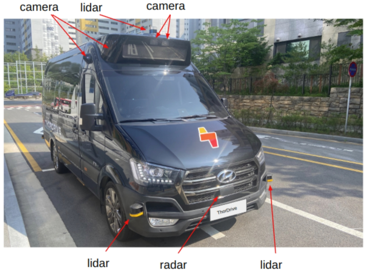
Figure 19: Test vehicle for the real-world experiment. The test vehicle is equipped with several lidars, radars, and cameras. The wheelbase is $3.72m$, and the minimum turning radius is $6m$.

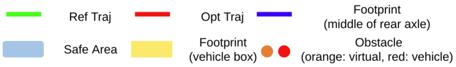
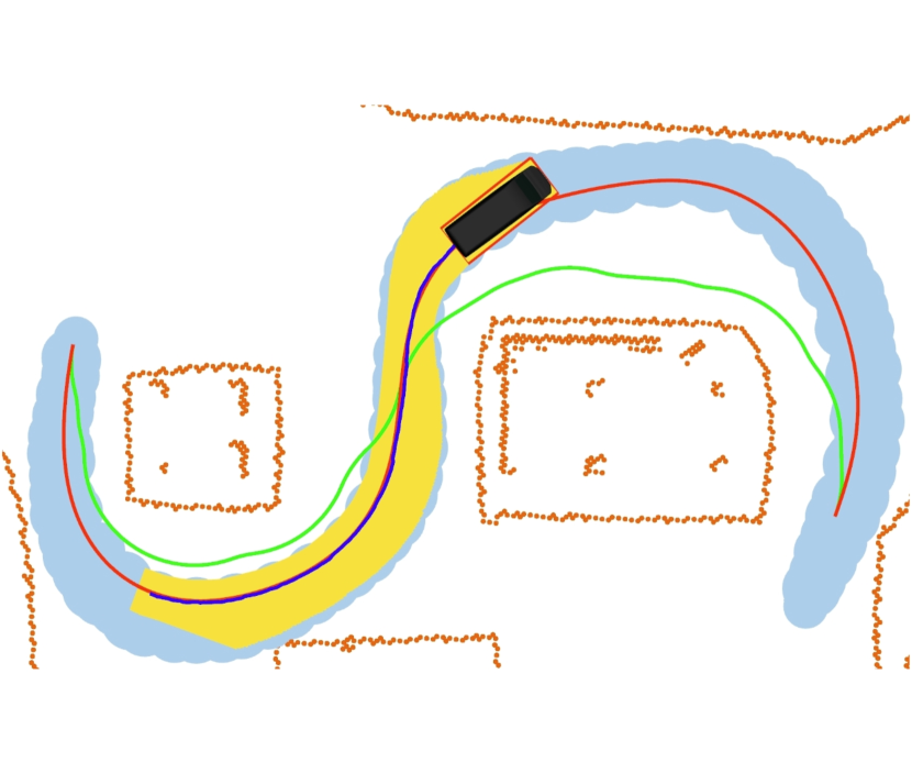
(a)

(b)

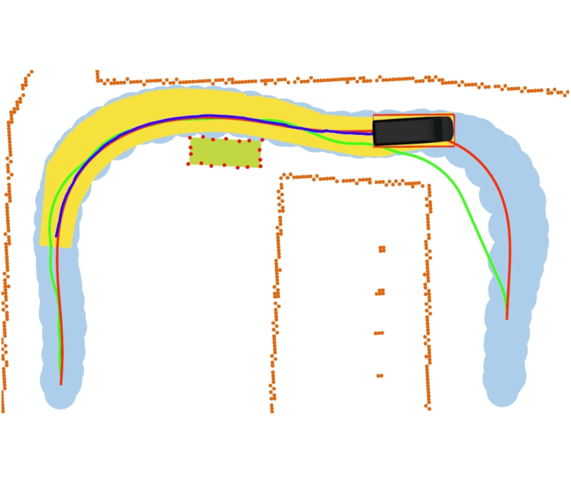
(c)

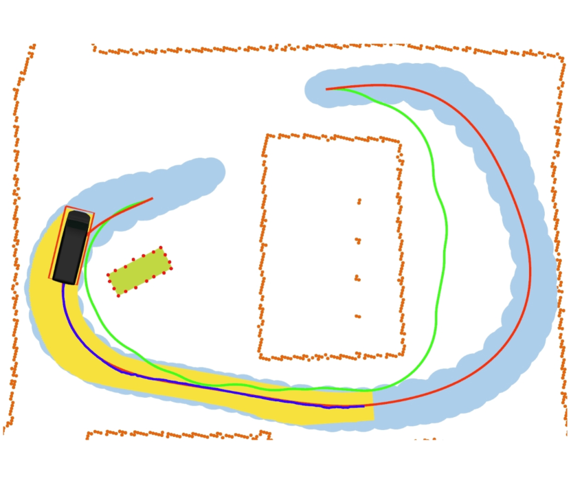
(d)

Figure 20: Four scenarios for the real-world experiments: (a) s-curve 1, (b) s-curve 2, (c) narrow corridor, (d) sharp turn.

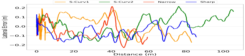
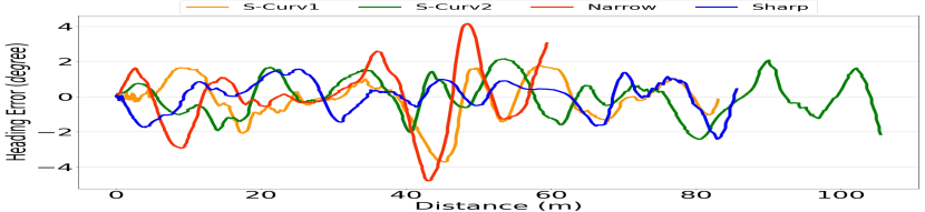
Figure 21: Lateral and heading errors in real world.

  Scenarios S-curve 1 S-curve 2 Narrow corridor Sharp turn   Max. Abs Long. Vel ($m/s)$ 1.9718 2.0524 2.4233 2.5633 Max. Abs Long. Acc ($m/s^{2}$) 1.4554 0.8802 1.1868 1.2832 Max. Abs Lat. Acc ($m/s^{2}$) 0.4169 0.4276 0.3784 0.4448 Max. Abs Curvature ($m^{-1})$ 0.1433 0.1478 0.1565 0.1426 Comp. Time ($ms$) 37.12 73.42 91.35 81.82  

TABLE IV: Actual vehicle status in real-world

We applied the proposed algorithm on a test vehicle, as shown in Fig. 19. It was a Hyundai Solati model with several sensors and an onboard computer (AMD Ryzen 7 series clocked at 2.2 GHz). We used the MPC controller from the simulation test and set the number of discs $\textsc{N}_{\textsc{DISC}}$ to $3$ to increase the safety buffer. The test site, as shown in Fig. 20, was an open outdoor space with static obstacles (virtual and vehicle), which were all detected before trajectory optimization. The virtual obstacles included predefined obstacles and nonmoving obstacles, which were detected by sensors. The vehicle obstacles, also detected by the sensors, were surrounded by multiple static obstacles. The objective of this experiment was to evaluate the tracking performance of the proposed method using a real vehicle. The vehicle could reach a given goal without collision.

Fig. 20 shows that the vehicle followed the optimized trajectory in four different scenarios: two s-curves, a narrow corridor, and a sharp turn. The lateral and heading errors in the four scenarios are plotted in Fig. 21. The errors in the last $2m$ were excluded from the plots because the controller had limitations in tracking short paths during the stopping phase, which is beyond the scope of this paper. These plots show that the lateral errors were between $-0.24$ and $+0.24m$ and the heading errors were between $-5.0$ and $4.5deg$, which were lower than the simulation results of the baselines in Fig. 17. Thus, the tracking performance of the proposed method was valid in the real world despite some errors caused by perception and localization in this setting. Furthermore, Table IV shows the actual vehicle status by following the optimized trajectory. The vehicle sped up to $2.56m/s$, and the velocity, acceleration, and curvature were bounded within the kinodynamic feasibility constraints, namely, longitudinal velocity ($m/s$): $[0,2.78]$; longitudinal acceleration ($m/s^{2}$): $[-2.0,2.0]$; lateral acceleration ($m/s^{2}$): $[-1.0,1.0]$; curvature constraint ($m^{-1}$): $[-1.67,1.67]$.

VII CONCLUSIONS

This study proposes a B-spline-based trajectory optimization method for AVs. This approach overcomes the difficulty on integrating vehicle kinodynamics on a B-spline-based trajectory optimization algorithm using an IPF, a disc type SV estimation method, and kinodynamic feasibility constraints. Simulation was conducted to show the effectiveness of the proposed methods compared with other SOTA algorithms. The simulation results demonstrated that the proposed method outperforms the SOTA algorithms in traceability, efficiency, and robustness. Furthermore, we conducted an experiment using a real vehicle and found that the simulated tracking performance of the proposed method was also valid in the real-world environment. In future work, we will use the proposed method with dynamic obstacles. As this approach is more efficient and robust than traditional trajectory optimization algorithms, a trajectory planning algorithm can be improved using this method.

Jongseo Choi received the B.S. degree in Electronic Engineering from Chungbuk National University, South Korea, in 2015. He received the M.S. degree in Automotive Software Engineering from Chemnitz University of Technology, Germany, in 2020. He was a quality engineer in the mechatronics quality department of Hyundai Mobis Co., Ltd., South Korea, from 2015 to 2018. He worked with IAV Automotive Engineering, Inc., Germany, as an intern researcher working on motion prediction for autonomous vehicles, from 2019 to 2020. Since 2020, he has been with ThorDrive Co., Ltd, Seoul, South Korea, as a senior researcher working on motion planning for autonomous driving. His research interests include motion planning and motion prediction for autonomous vehicles.

Hyuntai Chin received the B.E. and M.E. degrees in Mechanical Engineering from Nagoya University, Nagoya, Japan, in 2015 and 2017, respectively. In 2018, he was a visiting student researcher of Mechanical Engineering Department of U.C.Berkeley, United States working on cooperative adaptive cruise control. Since 2020, he has been with ThorDrive Co., Ltd, Seoul, South Korea, working on vehicle control for autonomous driving. His research interests include robust path and speed tracking, vehicle platooning, and optimal control.

Hyunwoo Park received the B.S. degree in mechanical engineering from Yonsei University, Seoul, South Korea, in 2022. He is currently working as a researcher in the Planning team at ThorDrive Co., Ltd, Seoul, South Korea. His research interests include motion planning for autonomous vehicles and machine learning.

Daehyeok Kwon received the B.S. degree in Electronic Engineering from Hanyang University, Seoul, South Korea, in 2018. He is currently pursuing the Ph.D. degree with the Department of Electrical Engineering and Computer Science, Seoul National University, Seoul, South Korea. He is also a Researcher with ThorDrive Co., Ltd, Seoul, South Korea. His current research areas include machine learning and autonomous driving.

Sanghyun Lee received the B.S. degree in automotive engineering from Hanyang University, Seoul, South Korea, in 2015, and the Ph.D. degree in electrical engineering and computer science from Seoul National University, Seoul, South Korea, in 2024. He was a senior researcher with ThorDrive Co., Ltd, Seoul, South Korea. His current research areas include reinforcement learning, imitation learning, robot learning, and autonomous driving.

Doosan Baek received the B.S. degree in the Department of Electrical Engineering from Seoul National University, Seoul, South Korea, in 2012. He is currently pursuing the Ph.D. degree in the Department of Electrical Engineering and Computer Science from Seoul National University, South Korea. He is also a CTO(Chief Technical Officer) at ThorDrive Co., Ltd, South Korea. His current research areas include the system architecture of autonomous driving, sensor fusion-based perception, localization, and calibration for autonomous vehicles.

References

- [1] W. Lim, S. Lee, M. Sunwoo, and K. Jo, “Hierarchical trajectory planning of an autonomous car based on the integration of a sampling and an optimization method,” IEEE Transactions on Intelligent Transportation Systems, vol. 19, no. 2, pp. 613–626, 2018.
- [2] J. Zhou, R. He, Y. Wang, S. Jiang, Z. Zhu, J. Hu, J. Miao, and Q. Luo, “Autonomous driving trajectory optimization with dual-loop iterative anchoring path smoothing and piecewise-jerk speed optimization,” IEEE Robotics and Automation Letters, vol. 6, no. 2, pp. 439–446, 2020.
- [3] H. Fan, F. Zhu, C. Liu, L. Zhang, L. Zhuang, D. Li, W. Zhu, J. Hu, H. Li, and Q. Kong, “Baidu apollo em motion planner,” arXiv preprint arXiv:1807.08048, 2018.
- [4] C. Rösmann, F. Hoffmann, and T. Bertram, “Kinodynamic trajectory optimization and control for car-like robots,” in 2017 IEEE/RSJ International Conference on Intelligent Robots and Systems (IROS). IEEE, 2017, pp. 5681–5686.
- [5] B. Li, Y. Zhang, Y. Ge, Z. Shao, and P. Li, “Optimal control-based online motion planning for cooperative lane changes of connected and automated vehicles,” in 2017 IEEE/RSJ International Conference on Intelligent Robots and Systems (IROS). IEEE, 2017, pp. 3689–3694.
- [6] R. He, J. Zhou, S. Jiang, Y. Wang, J. Tao, S. Song, J. Hu, J. Miao, and Q. Luo, “Tdr-obca: A reliable planner for autonomous driving in free-space environment,” in 2021 American Control Conference (ACC). IEEE, 2021, pp. 2927–2934.
- [7] B. Li, T. Acarman, Y. Zhang, Y. Ouyang, C. Yaman, Q. Kong, X. Zhong, and X. Peng, “Optimization-based trajectory planning for autonomous parking with irregularly placed obstacles: A lightweight iterative framework,” IEEE Transactions on Intelligent Transportation Systems, vol. 23, no. 8, pp. 11 970–11 981, 2021.
- [8] B. Li, Y. Ouyang, L. Li, and Y. Zhang, “Autonomous driving on curvy roads without reliance on frenet frame: A cartesian-based trajectory planning method,” IEEE Transactions on Intelligent Transportation Systems, vol. 23, no. 9, pp. 15 729–15 741, 2022.
- [9] X. Zhou, Z. Wang, H. Ye, C. Xu, and F. Gao, “Ego-planner: An esdf-free gradient-based local planner for quadrotors,” IEEE Robotics and Automation Letters, vol. 6, no. 2, pp. 478–485, 2020.
- [10] W. Ding, W. Gao, K. Wang, and S. Shen, “An efficient b-spline-based kinodynamic replanning framework for quadrotors,” IEEE Transactions on Robotics, vol. 35, no. 6, pp. 1287–1306, 2019.
- [11] B. Zhou, F. Gao, L. Wang, C. Liu, and S. Shen, “Robust and efficient quadrotor trajectory generation for fast autonomous flight,” IEEE Robotics and Automation Letters, vol. 4, no. 4, pp. 3529–3536, 2019.
- [12] C. De Boor and C. De Boor, A practical guide to splines. springer-verlag New York, 1978, vol. 27.
- [13] R. Deits and R. Tedrake, “Efficient mixed-integer planning for uavs in cluttered environments,” in 2015 IEEE international conference on robotics and automation (ICRA). IEEE, 2015, pp. 42–49.
- [14] Z. Zhu, E. Schmerling, and M. Pavone, “A convex optimization approach to smooth trajectories for motion planning with car-like robots,” in 2015 54th IEEE conference on decision and control (CDC). IEEE, 2015, pp. 835–842.
- [15] B. Li and Z. Shao, “Simultaneous dynamic optimization: A trajectory planning method for nonholonomic car-like robots,” Advances in Engineering Software, vol. 87, pp. 30–42, 2015.
- [16] X. Zhang, A. Liniger, and F. Borrelli, “Optimization-based collision avoidance,” IEEE Transactions on Control Systems Technology, vol. 29, no. 3, pp. 972–983, 2020.
- [17] B. Li and Z. Shao, “A unified motion planning method for parking an autonomous vehicle in the presence of irregularly placed obstacles,” Knowledge-Based Systems, vol. 86, pp. 11–20, 2015.
- [18] J. Schulman, Y. Duan, J. Ho, A. Lee, I. Awwal, H. Bradlow, J. Pan, S. Patil, K. Goldberg, and P. Abbeel, “Motion planning with sequential convex optimization and convex collision checking,” The International Journal of Robotics Research, vol. 33, no. 9, pp. 1251–1270, 2014.
- [19] H. Andreasson, J. Saarinen, M. Cirillo, T. Stoyanov, and A. J. Lilienthal, “Fast, continuous state path smoothing to improve navigation accuracy,” in 2015 IEEE International Conference on Robotics and Automation (ICRA). IEEE, 2015, pp. 662–669.
- [20] C. Liu, C.-Y. Lin, and M. Tomizuka, “The convex feasible set algorithm for real time optimization in motion planning,” SIAM Journal on Control and optimization, vol. 56, no. 4, pp. 2712–2733, 2018.
- [21] B. Li, T. Acarman, X. Peng, Y. Zhang, X. Bian, and Q. Kong, “Maneuver planning for automatic parking with safe travel corridors: A numerical optimal control approach,” in 2020 European Control Conference (ECC). IEEE, 2020, pp. 1993–1998.
- [22] A. Scheuer and T. Fraichard, “Continuous-curvature path planning for car-like vehicles,” in Proceedings of the 1997 IEEE/RSJ International Conference on Intelligent Robot and Systems. Innovative Robotics for Real-World Applications. IROS’97, vol. 2. IEEE, 1997, pp. 997–1003.
- [23] N. Ghita and M. Kloetzer, “Trajectory planning for a car-like robot by environment abstraction,” Robotics and Autonomous Systems, vol. 60, no. 4, pp. 609–619, 2012.
- [24] B. Li, Y. Zhang, T. Zhang, T. Acarman, Y. Ouyang, L. Li, H. Dong, and D. Cao, “Embodied footprints: A safety-guaranteed collision avoidance model for numerical optimization-based trajectory planning,” arXiv preprint arXiv:2302.07622, 2023.
- [25] T. Maekawa, T. Noda, S. Tamura, T. Ozaki, and K.-i. Machida, “Curvature continuous path generation for autonomous vehicle using b-spline curves,” Computer-Aided Design, vol. 42, no. 4, pp. 350–359, 2010.
- [26] M. Elbanhawi, M. Simic, and R. N. Jazar, “Continuous path smoothing for car-like robots using b-spline curves,” Journal of Intelligent & Robotic Systems, vol. 80, pp. 23–56, 2015.
- [27] T. Zhang, M. Fu, W. Song, Y. Yang, and M. Wang, “Trajectory planning based on spatio-temporal map with collision avoidance guaranteed by safety strip,” IEEE Transactions on Intelligent Transportation Systems, vol. 23, no. 2, pp. 1030–1043, 2020.
- [28] W. Ding, L. Zhang, J. Chen, and S. Shen, “Safe trajectory generation for complex urban environments using spatio-temporal semantic corridor,” IEEE Robotics and Automation Letters, vol. 4, no. 3, pp. 2997–3004, 2019.
- [29] R. Van Hoek, J. Ploeg, and H. Nijmeijer, “Cooperative driving of automated vehicles using b-splines for trajectory planning,” IEEE Transactions on Intelligent Vehicles, vol. 6, no. 3, pp. 594–604, 2021.
- [30] T. Mercy, R. Van Parys, and G. Pipeleers, “Spline-based motion planning for autonomous guided vehicles in a dynamic environment,” IEEE Transactions on Control Systems Technology, vol. 26, no. 6, pp. 2182–2189, 2017.
- [31] K. Qin, “General matrix representations for b-splines,” in Proceedings Pacific Graphics’ 98. Sixth Pacific Conference on Computer Graphics and Applications (Cat. No. 98EX208). IEEE, 1998, pp. 37–43.
- [32] H. Zhao, L. Zhu, and H. Ding, “A real-time look-ahead interpolation methodology with curvature-continuous b-spline transition scheme for cnc machining of short line segments,” International Journal of Machine Tools and Manufacture, vol. 65, pp. 88–98, 2013.
- [33] M. Elbanhawi, M. Simic, and R. N. Jazar, “Continuous path smoothing for car-like robots using b-spline curves,” Journal of Intelligent & Robotic Systems, vol. 80, pp. 23–56, 2015.
- [34] A. Ravankar, A. A. Ravankar, Y. Kobayashi, Y. Hoshino, and C.-C. Peng, “Path smoothing techniques in robot navigation: State-of-the-art, current and future challenges,” Sensors, vol. 18, no. 9, p. 3170, 2018.
- [35] R. B. Rusu and S. Cousins, “3d is here: Point cloud library (pcl),” in 2011 IEEE international conference on robotics and automation. IEEE, 2011, pp. 1–4.
- [36] S. Liu, M. Watterson, K. Mohta, K. Sun, S. Bhattacharya, C. J. Taylor, and V. Kumar, “Planning dynamically feasible trajectories for quadrotors using safe flight corridors in 3-d complex environments,” IEEE Robotics and Automation Letters, vol. 2, no. 3, pp. 1688–1695, 2017.
- [37] W. H. Press, W. T. Vetterling, S. A. Teukolsky, and B. P. Flannery, Numerical recipes. Citeseer, 1988.
- [38] A. Dosovitskiy, G. Ros, F. Codevilla, A. Lopez, and V. Koltun, “Carla: An open urban driving simulator,” in Conference on robot learning. PMLR, 2017, pp. 1–16.
- [39] J. Barzilai and J. M. Borwein, “Two-point step size gradient methods,” IMA journal of numerical analysis, vol. 8, no. 1, pp. 141–148, 1988.
- [40] R. S. Dembo and T. Steihaug, “Truncated-newton algorithms for large-scale unconstrained optimization,” Mathematical Programming, vol. 26, no. 2, pp. 190–212, 1983.
- [41] A. S. Lewis and M. L. Overton, “Nonsmooth optimization via quasi-newton methods,” Mathematical Programming, vol. 141, pp. 135–163, 2013.
- [42] D. Dolgov, S. Thrun, M. Montemerlo, and J. Diebel, “Path planning for autonomous vehicles in unknown semi-structured environments,” The international journal of robotics research, vol. 29, no. 5, pp. 485–501, 2010.
- [43] B. Stellato, G. Banjac, P. Goulart, A. Bemporad, and S. Boyd, “Osqp: An operator splitting solver for quadratic programs,” Mathematical Programming Computation, vol. 12, no. 4, pp. 637–672, 2020.
- [44] A. Wächter and L. T. Biegler, “On the implementation of an interior-point filter line-search algorithm for large-scale nonlinear programming,” Mathematical programming, vol. 106, pp. 25–57, 2006.
- [45] M.-Y. Yu, R. Vasudevan, and M. Johnson-Roberson, “Occlusion-aware risk assessment for autonomous driving in urban environments,” IEEE Robotics and Automation Letters, vol. 4, no. 2, pp. 2235–2241, 2019.
Glossary