Hemisphere-averaged Hellings-Downs curve between pulsar pairs for a gravitational wave source

Abstract

The Hellings-Downs (HD) curve plays a crucial role in search for nano-hertz gravitational waves (GWs) with pulsar timing arrays. We discuss the angular pattern of correlations for pulsar pairs within a celestial hemisphere. The hemisphere-averaged correlation curve depends upon the sky location of a GW compact source like a binary of supermassive black holes. If a single source is dominant, the variation in the hemisphere-averaged angular correlation is greatest when the hemisphere has its North Pole at the sky location of the GW source. Possible GW amplitude and source distance relevant to the current PTAs by using the hemisphere-averaged correlation are also studied.

I Introduction

Decades ago, the idea of using radio pulse timing to search for gravitational waves (GWs) was proposed Estabrook ; Sazhin ; Detweiler . Notably, Hellings and Downs (HD) pointed out that the angular correlation pattern for pulsar pairs averaged over the sky can provide an evidence of GWs Hellings , since the correlation curve is a consequence of the quadrupole nature of GWs CreightonBook ; MaggioreBook ; Anholm2009 ; Jenet . Along this direction, several teams of pulsar timing arrays (PTAs) have recently reported an evidence of nano-hertz GWs Agazie2023 ; Antoniadis2023 ; Reardon2023 ; Xu2023 . According to their results, superpositions of supermassive black hole binaries (SMBHBs) are among possible GW sources, though the origin of the significant correlation has not been identified yet. See e.g. Reference Romano for a review on detection methods of stochastic GW backgrounds.

For an isotropic stochastic background of GWs composed of the plus and cross polarization modes in general relativity, the expected correlated response of pulsar pairs follows the HD curve, where the averaging over the whole sky ($4\pi$) is taken. The whole-sky average makes the HD curve insensitive to any particular direction of the sky. This is the price of extracting tiny GW signals from large fluctuations of pulse signals from individual pulsars. Therefore, it is not surprising that an isolated SMBH binary produces an identical cross-correlation pattern as an isotropic stochastic background Cornish .

What happens in the pulsar correlation if the averaging domain is changed from the whole sky? Any deviation from the the whole-sky average breaks the isotropy. It may thus allow to use modified cross-correlation curves for the sky localization of a GW source.

The main purpose of this paper is to examine if the angular correlation pattern for pulsar pairs within a sky hemisphere has a dependence on a GW compact source. We show that, if a single GW source is dominant, the variation in a hemisphere-averaged angular correlation curve is greatest when the hemisphere has its North Pole at the sky location of the GW source.

This paper is organized as follows. Section II considers pulsar pairs within a sky hemisphere, for which the pulsar correlation curve is discussed. In section III, we discuss the dependence of the maximum correlation and the minimum one on the North Pole of a hemisphere. We shall show that the difference between the maximum and minimum correlations for a single hemisphere is greatest, if and only if the hemisphere has its North Pole at the sky location of the GW source. Section VI is devoted to Conclusion. Throughout this paper, $a$ and $b$ label two pulsars as a pair, and the center of the coordinates is the solar barycenter, safely approximated as the Earth.

II Hemisphere-averaged angular-correlation pattern

II.1 Full-sky cross-correlation

Following Reference CreightonBook ; MaggioreBook ; Anholm2009 , let us discuss a correlation of pulsar pairs. See e.g. Appendix C of Anholm2009 for detailed calculations of deriving the standard HD curve.

We consider a GW compact source which is chosen as the $z$ direction in the coordinates $(x,y,z)$. See Figure 1 for the GW-oriented coordinate system $(x,y,z)$. The fractional frequency shift in the timing observation of the $a$-th pulsar can be written as Hellings

$$\frac{\delta\nu_{a}}{\nu_{a}}=R_{a}h(t)+n_{a}(t),$$ (1)

where $h(t)$ is the GW signal, $n_{a}(t)$ is the noise, and the response $R_{a}=\cos 2\Phi_{a}(1+\cos\Theta_{a})$ for $\Theta_{a}\in[0,\pi)$ and $\Phi_{a}\in[0,2\pi)$.

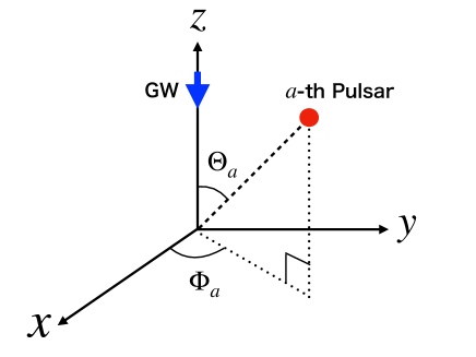
Figure 1: GW-oriented coordinates $(x,y,z)$. The GWs propagate downward along the $z$-axis. The latitude and longitude of the $a$-th pulsar are $\Theta_{a}$ and $\Phi_{a}$, respectively.

By taking the average over the sky, the cross-correlation of pulsar pairs is Hellings ; CreightonBook ; MaggioreBook ; Anholm2009

$$\Gamma_{\rm{S}}\equiv\frac{1}{4\pi}\int_{S}R_{a}R_{b}d\Omega,$$ (2)

where $S$ is the unit sphere and the noise terms are assumed to be uncorrelated. So far, Eq. (2) has been considered mostly for isotropic stochastic GW background CreightonBook ; MaggioreBook ; Anholm2009 ; Jenet ; Agazie2023 ; Antoniadis2023 ; Reardon2023 ; Xu2023 .

II.2 Hemisphere cross-correlation

Next, we consider a sky hemisphere $H$ in Figure 2. The North Pole $\rm{N}_{\rm{H}}$ is denoted as $\bm{N}_{\rm{H}}\equiv(\sin\alpha\cos\beta,\sin\alpha\sin\beta,\cos\alpha)$ and $\alpha$ is the inclination angle of the hemisphere from the GW source direction. Averaging over this hemisphere may be expressed as

$$\Gamma_{\rm{H}}\equiv\frac{1}{2\pi}\int_{H}R_{a}R_{b}d\Omega,$$ (3)

where a factor in front of the hemisphere integral is $1/2\pi$.

A practical problem is how to perform the integration, because $\Theta_{a}$ and $\Phi_{a}$ for the hemisphere case are allowed in a non-trivial domain, and thereby calculations of $\int_{\rm{H}}d\Omega=\int\sin\theta d\theta\int d\phi$ are not straightforward, because $\Theta_{a}$ and $\Phi_{a}$ do not respect the North Pole of the hemisphere. Therefore, the angle coordinates $\theta$ and $\phi$ shall be specified below to respect a hemisphere that we wish to study.

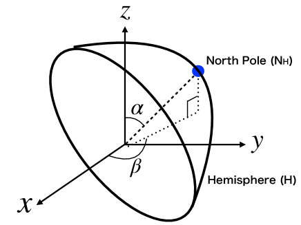
Figure 2: Hemisphere in the coordinates $(x,y,z)$. The latitude and longitude of the North Pole are $\alpha$ and $\beta$, respectively.

For the purpose of practical calculations of Eq. (3), therefore, it is convenient to introduce another coordinates $(x^{\prime},y^{\prime},z^{\prime})$ such that the North Pole is chosen as the $z^{\prime}$-axis. See Figure 3 for the new coordinates respecting the North Pole of a hemisphere. In the coordinates, the unit vector to the $a$-th pulsar can be written as $\bm{n}_{a}=(\sin\theta\cos\phi,\sin\theta\sin\phi,\cos\theta)$, for which the half sphere as $\theta\in[0,\pi/2)$ and $\phi\in[0,2\pi)$ fully agrees with the hemisphere.

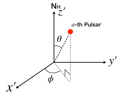
Figure 3: Hemisphere-oriented coordinates $(x^{\prime},y^{\prime},z^{\prime})$. The latitude and longitude of the $a$-th pulsar are $\theta$ and $\phi$, respectively.

II.3 Pulsar-oriented coordinates

The separation angle between the pulsar pair is denoted as $\gamma$. For clearly describing the configuration of the two pulsars, we introduce a third coordinate system $(X,Y,Z)$ such that the $a$-th pulsar location is chosen along the $Z$-axis. See Figure 4 for the coordinates $(X,Y,Z)$.

The $b$-th pulsar is located on a cone where the apex is the origin of the $(X,Y,Z)$ coordinates, the apex angle is $\gamma$, and the $a$-th pulsar is on the axis. In the third coordinate system, the $b$-th pulsar direction can be written as $\bm{n}_{b}=(\sin\gamma\cos\delta,\sin\gamma\sin\delta,\cos\gamma)$.

II.4 Transformations among the GW-oriented, Pulsar-oriented and Hemisphere-oriented coordinates

The coordinate transformation from $(x^{\prime},y^{\prime},z^{\prime})$ to $(x,y,z)$ is a composed rotation as

$$S=\begin{pmatrix}\cos\alpha\cos\beta&-\sin\beta&\sin\alpha\cos\beta\\ \cos\alpha\sin\beta&\cos\beta&\sin\alpha\sin\beta\\ -\sin\alpha&0&\cos\alpha\end{pmatrix},$$ (4)

and that from $(X,Y,Z)$ to $(x^{\prime},y^{\prime},z^{\prime})$ is

$$T=\begin{pmatrix}\cos\theta\cos\phi&-\sin\phi&\sin\theta\cos\phi\\ \cos\theta\sin\phi&\cos\phi&\sin\theta\sin\phi\\ -\sin\theta&0&\cos\theta\end{pmatrix}.$$ (5)

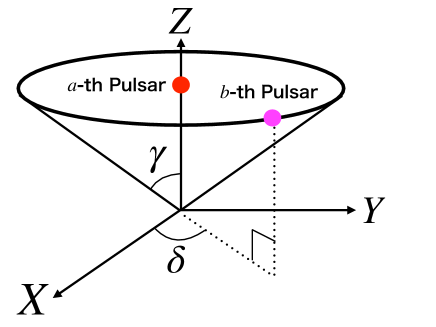
Figure 4: Pulsar-oriented coordinates $(X,Y,Z)$ and the separation angle $\gamma$ between the $a$-th pulsar and the $b$-th one. The $b$-th pulsar is on a cone and its direction is specified by two angles $\gamma$ and $\delta$.

In the $(x,y,z)$ coordinate representation, the $a$-th and $b$-th pulsar directions are $\bm{n}_{a}=S(\sin\theta\cos\phi,\sin\theta\sin\phi,\cos\theta)^{\mbox{T}}$, and $\bm{n}_{b}=ST(\sin\gamma\cos\delta,\sin\gamma\sin\delta,\cos\gamma)^{\mbox{T}}$, where the superscript T denotes the transposition.

II.5 Hemisphere cross-correlation II

The response $R_{A}(A=a,b)$ for the plus and cross modes of GWs coming from the direction $\bm{\Omega}$ can be rewritten in the covariant form as Anholm2009 ; Romano

$$R_{A}^{+} =\frac{1}{2}\frac{(\bm{n}_{A}\cdot\hat{\bm{\ell}})^{2}-(\bm{n}_{A}\cdot\hat{\bm{m}})^{2}}{1+\bm{\Omega}\cdot\bm{n}_{A}}$$

$$R_{A}^{\times} =\frac{(\bm{n}_{A}\cdot\hat{\bm{\ell}})(\bm{n}_{A}\cdot\hat{\bm{m}})}{1+\bm{\Omega}\cdot\bm{n}_{A}},$$ (6)

where $\hat{\bm{\ell}}=(0,-1,0)$ and $\hat{\bm{m}}=(-1,0,0)$ in the the $(x,y,z)$ coordinates are the orthonormal bases on the plane perpendicular to the GW propagation and $\hat{\bm{\ell}}$ and $\hat{\bm{m}}$ can be used in the definition of the plus and cross modes.

Therefore, the total correlation by both the plus and cross modes is Anholm2009 ; Romano

$$\Gamma_{\rm{H}}(\alpha,\beta,\gamma)=\frac{1}{(2\pi)^{2}}\int_{0}^{2\pi}d\delta\int_{H}(R_{a}^{+}R_{b}^{+}+R_{a}^{\times}R_{b}^{\times})d\Omega,$$ (7)

where the $a$-th pulsar is averaged on the hemisphere ($(1/2\pi)\int d\Omega$), and the $b$-th pulsar is averaged over the cone ($(1/2\pi)\int d\delta$). The denominator in front of the integrals is $2\pi(\rm{hemisphere})\times 2\pi(\rm{\delta\;integral})=4\pi^{2}$.

After substituting Eq. (6) into Eq. (7), the integrand is a function of six angles $\alpha,\beta,\gamma,\delta,\theta,\phi$. For the average over the present hemisphere, Eq. (7) explicitly becomes

$$\Gamma_{\rm{H}}(\alpha,\beta,\gamma)$$

$$= \frac{1}{4\pi^{2}}\int_{0}^{2\pi}d\delta\int_{0}^{2\pi}d\phi\int_{0}^{\pi/2}\sin\theta d\theta(R_{a}^{+}R_{b}^{+}+R_{a}^{\times}R_{b}^{\times}).$$ (8)

In the present formulation, we do not need take special care of the integration domain, whereas Eq. (3) needs a special care for a hemisphere case because the GW propagation axis is not aligned with the polar axis of a hemisphere.

In this paper, the integration in Eq. (8) is done numerically for a hemisphere, whereas the correlation integration can be done analytically for the full sky Hellings ; Anholm2009 .

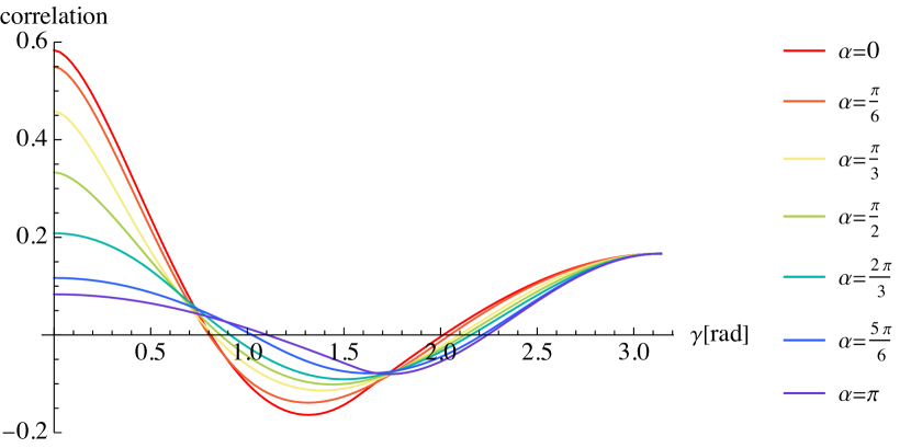
Figure 5: Hemisphere-averaged angular-correlation pattern for pulsar pairs. It depends upon an inclination angle $\alpha$, which runs from $0^{\circ}$ to $180^{\circ}$ every 30 degrees. The separation angle viewed from the Earth is $\gamma$.

III GW sky location and the maximum and minimum correlations

III.1 Angular correlation pattern for a hemisphere

Numerical calculations of Eq. (8) give angular correlation patterns. It follows that the curves depend upon $\alpha$ but not upon $\beta$, because they are symmetric around the propagation axis of GWs. See Figure 5 for the numerical plots.

The angular correlation pattern for a hemisphere has a rotational symmetry around the polar axis of the hemisphere. Therefore, the plot for $\alpha=\pi/2$ in Figure 6 is accidentally the same as the standard HD curve, though the former curve is for a hemisphere and the latter one is for the whole sky. The reason for this coincidence is that only the $\alpha=\pi/2$ has pulsars in the north and south skies in the same proportion (a half) to the whole sky in the HD curve.

At $\gamma=0$, the correlation decreases as $\alpha$ increases. This is because as the hemisphere is more inclined with respect to the GW axis, $\Theta_{a}$ of pulsars in the hemisphere are larger and hence the response $R_{a}$ is smaller.

The maximum correlation $\Gamma_{\rm{max}}$ for each value of $\alpha$ monotonically decreases as $\alpha$ increases. On the other hand, the minimum correlation $\Gamma_{\rm{min}}$ monotonically increases. Therefore, the difference between the maximum and minimum correlations ($\Delta\Gamma\equiv\Gamma_{\rm{max}}-\Gamma_{\rm{min}}$) is more sensitive to $\alpha$ than either of $\Gamma_{\rm{max}}$ and $\Gamma_{\rm{min}}$.

III.2 Source localization in the sky

$\Delta\Gamma$ is maximized in the direction of the GW source on the sky. See Figure 6 for a contour sky map of $\Delta\Gamma$. This figure shows that the position of the maximum $\Delta\Gamma$ perfectly agrees with the GW sky location. The contours have no dependence on the angle $\beta$ as a consequence of the averaging over each hemisphere as mentioned above. Plots such as Figures 5 and 6 from future observation data could potentially suggest the existence of a GW compact source with an allowed region in the sky.

What is the expected accuracy of the GW sky localization by using the hemisphere cross-correlation? For its simplicity, we assume the measurement accuracy of the cross-correlation, say $10$ percents, which means roughly the error in $\Delta\Gamma\sim O(0.1)$. According to Figure 6, the accuracy for the determined latitude (corresponding to $\alpha$) is nearly 10-20 degrees. This is not enough for pointing a host galaxy that may include a relevant GW source like a binary of supermassive black holes.

In the above discussion, we know the GW direction a priori. How can we use the hemisphere-averaged correlation for a GW source localization from future PTA observations? For instance, we prepare a set of hemispheres, e.g. 12 latitudes and 24 longitudes (by 15 degree step). For $12\times 24=288$ hemispheres, we estimate $\Delta\Gamma$. The maximum $\Delta\Gamma$ could indicate the GW location in the sky.

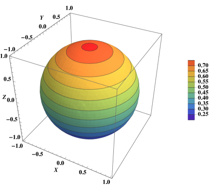
Figure 6: Contour map of the difference between the maximum and minimum correlations $\Delta\Gamma$. For its simplicity, the North Pole is chosen as the direction of a GW source.

III.3 On the hemisphere

Is there a caveat in a half size of the full sky? In their pioneering work Hellings , it was pointed out that a total number of pulsar pairs should be increased for statistically increasing the signal-to-noise ratio, because fluctuations of timings of individual pulsars are not so negligible. The maximum number of the pairs is available for the whole sky ($4\pi$). For $N_{\rm{pulsar}}$ as the total number of the observed pulsars in PTAs, the number of pulsars in the present method is nearly a half of $N_{\rm{pulsar}}$, where the isotropic distribution of pulsars is simply assumed. From the full sky to the hemisphere, the number of the pairs is reduced from $(N_{\rm{pulsar}})(N_{\rm{pulsar}}-1)/2$ to $(N_{\rm{pulsar}}/2)(N_{\rm{pulsar}}/2-1)/2$. For $N_{\rm{pulsar}}\gg 1$, this means from $(N_{\rm{pulsar}})^{2}/2$ to $(N_{\rm{pulsar}})^{2}/8$. Namely, it becomes one fourth, so that the statistical error increases twofold. For the current level of statistics in PTAs Agazie2023 ; Antoniadis2023 ; Reardon2023 ; Xu2023 , the hemisphere method may thus be a little challenging.

III.4 Relevant GW amplitude and source distance

How large is the GW amplitude relevant to the hemisphere-method? For estimating it, we use Eq. (1) to obtain the correlation of pulsar pairs as Hellings

$$\langle z_{a}z_{b}\rangle\sim\Gamma_{\rm{H}}\langle h^{2}\rangle,$$ (9)

where $z_{a}$ and $z_{b}$ denote the redshifts of pulse signals from the a-th and b-th pulsars, respectively, $\langle\quad\rangle$ denotes the autocorrelation, and $\langle n_{a}h\rangle=0$ and $\langle n_{a}n_{b}\rangle$. Roughly estimating, $z_{a}\sim\Delta t_{a}/T_{\rm{obs}}$, where $\Delta t_{a}$ is the delay from the expected arrival time and $T_{\rm{obs}}$ denotes the observation duration. In PTA observations, $T_{\rm{obs}}$ is roughly the inverse of the relevant GW frequency $f_{\rm{GW}}$. Hence, $z_{a}\sim z_{b}\sim(\Delta t_{a}/T_{\rm{obs}})\sim f_{\rm{GW}}\Delta t_{a}$, which leads to the variance of the cross correlation $\langle z_{a}z_{b}\rangle$ as $[\sigma(\langle z_{a}z_{b}\rangle)]^{2}\sim(N_{\rm pair})^{-1}(\Delta t_{a}/T_{\rm{obs}})^{4}$ for $N_{\rm pair}$ pairs of the pulsars. The standard deviation is roughly $\sigma(\langle z_{a}z_{b}\rangle)\sim(N_{\rm pulsar})^{-1}(\Delta t_{a}/T_{\rm{obs}})^{2}$, where $N_{\rm pair}\sim(N_{\rm pulsar})^{2}$. The $\alpha$-dependence of the hemisphere correlation can be detected when $\sigma(\langle z_{a}z_{b}\rangle)\lesssim(\delta_{\alpha}\Gamma_{\rm{H}})\langle h^{2}\rangle$, where $\delta_{\alpha}\Gamma_{\rm{H}}$ denotes the size of the variation of $\Gamma_{\rm{H}}$ for changing $\alpha$.

Therefore, the GW amplitude possibly relevant to the current PTAs by using the hemisphere-averaged correlation is roughly estimated as

$$h \sim\sqrt{\langle h^{2}\rangle}$$

$$\gtrsim 10^{-14}\left(\frac{10^{2}}{N_{\rm{pulsar}}}\right)^{1/2}\left(\frac{f_{\rm{GW}}}{1\rm{yr}^{-1}}\right)\left(\frac{\Delta t_{a}}{1\mu\rm{sec.}}\right)\left(\frac{0.1}{\delta_{\alpha}\Gamma_{\rm{H}}}\right)^{1/2},$$ (10)

where $\delta_{\alpha}\Gamma_{\rm{H}}$ is $\sim 0.1$, and the average accuracy in the time residual measurement is $O(1)\;\mu\rm{sec}$.

From Eq. (10), a nearby GW source can be marginally detected when the distance $D$ to the source is

$$D\lesssim 10{\rm Mpc}\left(\frac{N_{\rm{pulsar}}}{10^{2}}\right)^{1/2}\left(\frac{1\mu\rm{sec.}}{\Delta t_{a}}\right)\left(\frac{\delta_{\alpha}\Gamma_{\rm{H}}}{0.1}\right)^{1/2}$$

$$~{}~{}~{}~{}~{}\times\left(\frac{M}{10^{9}M_{\odot}}\right)^{5/3}\left(\frac{1{\rm yr}^{-1}}{f_{\rm GW}}\right)^{1/3},$$ (11)

where the quadrupole formula for a binary is used as $h\sim(MR^{2})/(DT^{2})\sim M^{5/3}(f_{\rm GW})^{2/3}/D$ for the total mass $M$, the orbital radius $R$, the orbital period $T$ ($T\sim 2/f_{\rm GW}$) CreightonBook ; MaggioreBook . On the other hand, a lower bound on the distance to the dominant source can be placed, unless $\delta_{\alpha}\Gamma_{\rm{H}}$ is detected.

The near future SKA would significantly improve the sensitivity of PTAs by a factor $\sim 5$ or more through newly finding hundreds of millisecond pulsars SKA . In the SKA era, the hemisphere method can be thus expected for e.g. the Coma cluster at $\sim 100$ Mpc.

III.5 Multiple sky locations of GWs

Before closing this section, we briefly mention the number of GW sources relevant to the cross-correlation curve. The present paper assumes a single GW source. How can the hemisphere cross-correlation curve be modified, if multiple GW compact sources are dominant in the cross-correlation curves? In the forthcoming PTA observations, GW frequencies from multiple strong GW sources (if they exist) are likely to be distinguishable from each other, since it is less feasible that the orbital period of one of SMBHSs is accidentally the same as that of another one. Here, what we mean by a strong GW source is that it can make signals larger than the stochastic GW background.

For each source with a different GW frequency, the hemisphere cross-correlation method can be used separately, if the number of the sources is not large, say a few. For more than a dozen of strong GW sources, two or more GW sources are degenerate in Fourier spaces. For such a case, the hemisphere method needs significant improvement by simultaneous inclusion of multiple sources. Detailed investigations taking account of two or more GW compact sources are beyond the scope of this paper.

Finally, we mention the term within the hemisphere. In the above formulation, most of pulsar pairs in the same hemisphere are taken into account. Exactly speaking, however, both components of a pair of pulsars do not need live in the hemisphere simultaneously; there can be a case that one of the pair is in H but the other is outside. The latter case is very rare for small $\gamma$, while it is a larger fraction for large $\gamma$. On the other hand, Eq. (3) cannot be calculated, unless a pulsar pair within a hemisphere is clearly defined in terms of the GW-oriented coordinates $(x,y,z)$.

The present result has an interesting implication. The distribution of pulsars observed by the current PTAs Agazie2023 ; Antoniadis2023 ; Reardon2023 ; Xu2023 is highly anisotropic, because we do not live in the galactic center. The deviation from the ideal HD curve in the current PTA observations Agazie2023 ; Antoniadis2023 ; Reardon2023 ; Xu2023 could be due to the anisotropic distribution of pulsars for a possible GW point-like source, though the deviation has not been established statistically. It would be interesting to pursue this direction further.

IV Conclusion

We discussed the hemisphere-averaged angular correlation pattern to pulsar pairs. Our numerical calculations showed that, if a single GW source is dominant, the variation in a hemisphere-averaged angular correlation curve is greatest when the hemisphere has its North Pole at the sky location of the GW source. Possible GW amplitude and source distance relevant to the current PTAs by using the hemisphere-averaged correlation were investigated. The near future SKA will make it possible to perform sky localization by using the hemisphere-averaged correlations.

We mention also the validity of the present method. We confirmed numerically that, regardless of $\alpha$ and $\beta$, Eq. (8) for the whole sky perfectly recovers the standard HD curve, if $\theta$ runs from $0$ to $\pi$ in the integration by $\theta$.

The hemisphere condition adopted in the present paper is that at least one pulsar of a pulsar pair is in the hemisphere. Another option is that both pulsars in a pair are located within the same hemisphere. It would be interesting to use such an option to examine which condition is more suitable for the sky localization. It is left for future.

V Acknowledgments

We are grateful to Daisuke Yamauchi, Yousuke Itoh, Keitaro Takahashi and Yuuiti Sendouda for useful discussions. We thank Yuya Nakamura and Ryuya Kudo for helpful suggestions on the numerical plots. This work was supported in part by Japan Society for the Promotion of Science (JSPS) Grant-in-Aid for Scientific Research, No. 20K03963 (H.A.).

References

- (1) F. B. Estabrook, and H. D. Wahlquist, General Relativ. Grav., 6, 439 (1975).
- (2) M. V. Sazhin, Soviet Ast., 22, 36 (1978).
- (3) S. Detweiler, Astrophys. J. 234, 1100 (1979).
- (4) R. W. Hellings, and G. S.Downs, Astrophys. J. Lett, 265, L39 (1983).
- (5) J. D. E. Creighton, and W. G. Anderson, Gravitational-Wave Physics and Astronomy: An Introduction to Theory, (Wiley, NY 2013).
- (6) M. Maggiore, Gravitational Waves: Astrophysics and Cosmology (Oxford Univ. Press, UK, 2018).
- (7) M. Anholm, S. Ballmer, J. D. E. Creighton, L. R. Price, and X. Siemens, Phys. Rev. D 79, 084030 (2009).
- (8) F. A. Jenet, and J. D. Romano, Am. J. Phys. 83, 635 (2015).
- (9) G. Agazie, et al., Astrophys. J. Lett. 951, L8 (2023).
- (10) J. Antoniadis, et al., Astron. Astrophys. 678, A50 (2023).
- (11) D. J. Reardon, et al., Astrophys. J. Lett. 951, L6 (2023).
- (12) H. Xu, et al., Res. Astron. Astrophys. 23, 075024 (2023).
- (13) J. D. Romano, and N. J. Cornish, Living Rev. Relativ. 20, 2 (2017).
- (14) N. J, Cornish, and A. Sesana, Class. Quantum Grav. 30, 224005 (2013).
- (15) https://www.skao.int/