Multi-band analysis of strong gravitationally lensed post-blue nugget candidates from the Kilo-Degree Survey

Abstract

During the early stages of galaxy evolution, a significant fraction of galaxies undergo a transitional phase between the “blue nugget” systems, which arise from the compaction of large, active star-forming disks, and the “red nuggets”, which are red and passive compact galaxies. These objects are typically only observable with space telescopes, and detailed studies of their size, mass, and stellar population parameters have been conducted on relatively small samples. Strong gravitational lensing can offer a new opportunity to study them in detail, even with ground-based observations. In this study, we present the first 6 bona fide sample of strongly lensed post-blue nugget (pBN) galaxies, which were discovered in the Kilo Degree Survey (KiDS). By using the lensing-magnified luminosity from optical and near-infrared bands, we have derived robust structural and stellar population properties of the multiple images of the background sources. The pBN galaxies have very small sizes ($<1.3$ kpc), high mass density inside 1 kpc ($\log\Sigma_{1}/M_{\odot}\mathrm{kpc}^{-2}>9.3$), and low specific star formation rates ($\log\mathrm{sSFR/Gyrs}\lesssim 0.5$), which places them between the blue and red nugget phases. The size-mass and $\Sigma_{1}$-mass relations of this sample are consistent with those of the red nuggets, while their sSFR is close to the lower end of compact star-forming blue nugget systems at the same redshift, suggesting a clear evolutionary link between them.

1 Introduction

According to the galaxy formation scenario (e.g., Renzini 2006; Lapi et al. 2018), large primordial disk galaxies undergo a dissipative process in which gas streams from the cosmic web fall into the disks, concentrate in the central region, and lead to a high rate of star formation (Dekel et al. 2009). This process results in the formation of extremely compact and star-forming galaxies, known as “blue nuggets” (Barro et al. 2013, 2014, Zolotov et al. 2015, Tacchella et al. 2016). They are characterized by a very small effective radius ($\rm R_{eff}<1\ kpc$; e.g., Williams et al. 2014; Zolotov et al. 2015), high surface density inside the central 1 kpc ($\rm log\Sigma_{1}>9.0\ M_{\odot}/kpc^{2}$; e.g. Barro et al. 2013; Dekel & Burkert 2014), and a high specific star-forming rate ($\rm log\ sSFR>0\ M_{\odot}Gyr^{-1}$; e.g., Zolotov et al. 2015; Huertas-Company et al. 2018). The lifetime of these blue nuggets can be quite short ($\rm<1\ Gyr$), as they are expected to quickly switch off their star formation ($\rm log\ sSFR\lesssim 0\ M_{\odot}Gyr^{-1}$) and turn into post-blue nuggets (pBNs) of similar structural properties (Dekel & Burkert 2014; Zolotov et al. 2015) but lower star forming rate. The actual mechanisms behind these “quick” transformations are yet to be clarified. They are thought to consist of the combined effect of feedback from star winds induced by strong starbursts and the presence of Active Galactic Nuclei (AGN) (e.g., Dekel & Silk 1986; Murray et al. 2005; Zolotov et al. 2015; Cattaneo et al. 2009). These mechanisms should be effective over a short timescale ($\sim$ 1 Gyr or less) and at higher redshifts ($z>2$, Dekel & Burkert 2014; Costantin et al. 2021). After complete quenching, the pBNs turn into compact red nuggets, which finally grow in mass and size through dry merging, forming present-day elliptical galaxies (e.g., Newman et al. 2012; Oser et al. 2012; Nipoti et al. 2012; Posti et al. 2014; Spiniello et al. 2021).

If the red nuggets indeed evolved from blue nuggets, there must be a continuum between some basic properties (e.g. mass, age, star-forming rate–SFRs, size and surface density inside 1 kpc–$\Sigma_{1}$, see e.g. Tacchella et al. 2016) of blue nuggets, pBNs and red nuggets (see e.g. Huertas-Company et al. 2018). Hence studying the relationships between these properties (e.g. size-mass, SFR-$\Sigma_{1}$, and size-$\Sigma_{1}$, e.g. Barro et al. 2014, 2017) can help us better understand their evolutionary path and determine their roles in the galaxy evolution scenario. This evolutionary track has been investigated in simulations by Zolotov et al. (2015), showing that the majority of compaction of blue nuggets when $\rm log(M_{*}/M_{\odot})<9.5$ and $\rm R_{eff}>1\ kpc$, followed by quenching at $\rm log(M_{*}/M_{\odot})\sim 10$ and $\rm R_{eff}<1\ kpc$. This compaction phase occurs up to $z\sim 2$. Furthermore, galaxies with larger mass experience quenching at a higher value of $\Sigma_{1}$, whereas lower mass galaxies quench at lower values of $\Sigma_{1}$. As blue nuggets transit into red nuggets, their size begins to increase linearly with mass along the passive galaxy size-mass relation. On the observational side, the size-mass relation of red nuggets has been investigated through direct observations (e.g. Damjanov et al. 2009) or the strong lensing magnification effect (Oldham et al. 2017). Although a few blue nuggets have also been found and confirmed (Marques-Chaves et al. 2022), their size-mass relation remains poorly constrained (see e.g. Williams et al. 2014), mainly because the sizes of this kind of galaxies are difficult to measure.

Strong lensing (SL), can provide powerful observational support to systematically study these objects. The warped geometry of the space and time generated by the gravitational field of massive objects (lenses) in the universe, produces a magnification of the luminosity of the background “lensed” galaxies. This is particularly efficient for compact sources, which can be studied in much higher detail (Oldham et al. 2017), even with ground-based observations (Napolitano et al. 2020). For example, Toft et al. (2017) analyzed a strongly lensed red nugget and suggested that the stars in this galaxy formed in a disk rather than a merger-driven nuclear starburst. Two Einstein crosses from post-blue nuggets have been discovered in the Kilo Degree Survey (KiDS, de Jong et al. 2013) and confirmed with VLT/MUSE observations by Napolitano et al. (2020, hereafter N+20). In this case, the magnification effect of strong lensing, combined with the 9-band optical images from KiDS and the near-infrared (NIR) images from the VISTA Kilo-degree Infrared Galaxy (VIKING) survey, enabled the accurate reconstruction of the light distribution of the lensed sources and computation of their stellar population properties. This analysis has shown the path for systematic studies of pBNs in quadruply lensing events in future ground and space large sky surveys, where thousands of similar systems have been predicted to be found (see a discussion in N+20).

Here we expand the sample of pBNs in the KiDS survey by adding four new candidates. For the first time, we use a full optical plus near-infrared ray tracing analysis to derive the photometric redshifts of the lenses and the sources, which allow us to photometrically demonstrate the lensing nature of the systems. Additionally, we perform a stellar population analysis of the sources by fitting the spectral energy distribution (SED) to determine the specific star-formation rate of the background galaxies and assess the pBN nature of the sources. The final sample of the bona fide pBNs is shown in Fig. 1, which includes the two systems previously analyzed in N+20 (KiDSJ122456$+$005048 and KiDSJ232940$-$340922) and four new systems (KiDSJ023929$-$321129, KiDSJ224546$-$295559, KiDSJ230226$-$335637, and KiDSJ234804-302855).

This sample, if confirmed, is consistent with the number of events predicted in the full KiDS area from N+20. Hence the primary objective of this paper is to confirm these candidates and characterize the properties of the sources. This will further allow us to compare their scaling relations with samples of blue and red nuggets from previous literature and find proof of their evolutionary link.

The paper is organized as follows. Section 2 describes the data used in this study. Section 3 outlines the main methods used for lens modelling, photometric redshift estimation, and determination of stellar population parameters. Section 4 discusses the multi-band ray-tracing results and the scaling relations of the six pBN candidates. Finally, Section 5 draws the conclusions of our study. For all calculations, we assume a $\Lambda$CDM cosmology with ($\Omega_{M}$, $\Omega_{\Lambda}$, $h$)=(0.3, 0.7, 0.7).

Figure 1: Colored stamps ($20^{\prime\prime}\times 20^{\prime\prime}$) of the six lensed blue nuggets, obtained by combining g, r, and i-band images from KiDS. Each system exhibits three or four point-like images, indicating that the background sources may be very small in size. The two systems highlighted in red have been confirmed with MUSE/VLT spectroscopy in N+20.

2 Data

Using deep learning, we have found 268 high-quality strong lens candidates in KiDS (Petrillo et al. 2019; Li et al. 2020, 2021). To collect the lensed pBNs candidates we have visually inspected the $gri$ composited stamps of these candidates and found that 14 of them have blue lensed images with at least one point-like lensed image, suggesting compact sizes of the background objects, similar to the lensed pBNs in N+20. Among these 14 candidates, two systems have more than one foreground deflector, which would make the lens modelling very uncertain. Furthermore, 6 of the remaining 12 candidates have an insufficient signal-to-noise ratio in at least three NIR bands, which we need for our analysis. This is partially because of the shallower depth of the VIKING data, but also for the combination of redshift and SED distribution of the background sources, which tend to be fainter in NIR if they are younger rather than older systems, at high-$z$ (see also in Williams et al. 2014, Fig. 17). The limiting magnitude of the VIKING survey is $\rm mag_{AB}<23$. Therefore, the star-forming galaxies with optical band magnitudes around 23-24 will be hard to detect even if they are magnified by lensing. This is an important selection effect to keep in mind in the following analysis. Finally, we are left with 6 SL systems with optical+NIR imaging data good enough for the analysis we aim to perform in this work. In Fig. 1 we show the $gri$ color combined images of the final 6 SL systems which we will use for this analysis. KiDSJ122456+005048 and KiDSJ232940-340922 are the pBNs observed with MUSE spectroscopy from N+20. We keep these “confirmed” cases in the sample to check if, with the pure photometric approach proposed here, we obtain consistent results in terms of redshift of the lens and the source. We also note that KiDSJ023929+321129 was studied by Sergeyev et al. 2018 as a gravitational quadruple lens candidate, without giving the redshift of the sources.

Table 1: Source properties from the multi-band ray tracing “flexible” model

ID	$R_{\rm eff}$	$b/a$	$pa$	n	u	g	r	i	Z	Y	J	H	Ks
	(arcsec)		(deg)		(mag)	(mag)	(mag)	(mag)	(mag)	(mag)	(mag)	(mag)	(mag)
J023929$-$321129	0.063$\pm$0.002	0.40$\pm$0.02	89	2.7$\pm$0.1	23.70	23.29	23.14	23.21	23.08	23.44	22.48	22.49	22.11
J122456$+$005048*	0.057$\pm$0.002	0.53$\pm$0.04	163	0.8$\pm$0.1	-	24.05	23.67	23.14	22.52	22.24	21.91	21.88	21.67
J224546$-$295559	0.054$\pm$0.006	0.46$\pm$0.05	16	3.4$\pm$0.5	24.02	23.90	23.73	23.72	23.20	22.79	22.62	-	-
J230226$-$335637	0.154$\pm$0.008	0.52$\pm$0.05	61	1.8$\pm$0.3	23.38	22.89	22.96	22.74	22.94	22.62	22.14	21.89	22.56
J232940$-$340922*	0.071$\pm$0.011	0.26$\pm$0.08	161	1.1 $\pm$0.2	-	23.68	23.52	23.53	23.39	22.86	22.52	22.12	21.86
J234804$-$302855	0.144$\pm$0.007	0.38$\pm$ 0.03	71	1.5$\pm$0.2	23.93	23.70	23.88	23.78	24.38	23.55	23.22	22.83	-

Note. — Column 1 is the KiDS ID, in the form of hh-mm-ss and deg-mm-ss. Columns 2-5 list the source parameters from the lensing model by assuming a Sérsic profile for the sources. From left to right are the $r-$band magnitude $r_{mag}$, the effective radius $R_{\rm eff}$ in the unit of arcsec, the minor-to-major axis ratio $b/a$, the position angle $pa$ and the Sérsic index $n$, respectively. Columns 6-14 list the magnitudes of each source obtained from the “flexible” lensing model (see text for details). Errors in magnitudes are shown in Fig. 3.

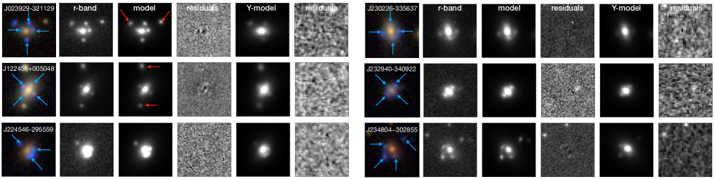
Figure 2: Ray tracing model of the selected systems shown in Fig. 1. From the left to right: 1) the color image; 2) the $r$-band image; 3) the Lensed $r$-band image model; 4) the $r$-band model-subtracted image; 5) the $Y$-band image model; 6) the $Y$-band model-subtracted image. The blue arrows point to the lensed images while the red arrows show other projected galaxies in the field-of-view.

3 Methods and model parameters

In this section we describe the methods adopted to 1) perform the ray tracing of the systems in optical and NIR images; 2) derive the structural parameters of the background sources; 3) use the “unlensed” multi-band photometry and colours to estimate the photometric redshifts and the stellar population parameters of the sources; 4) use the source decontaminated fluxes of the deflectors to obtain their photometric redshifts. Following N+20, we expect these systems to show high-$z$ ($z>1$), blue, ultra-compact sources with sSFR compatible with quenched systems.

3.1 Lens Modeling

For the ray tracing modelling of the optical and NIR bands, we use Lensed (Tessore et al. 2016), which implements a MCMC method to look for the best fitting parameters of the mass of the deflectors and the light of both the deflector and sources. The lensing model is convolved with a point spread function (PSF) obtained by fitting one nearby star to the lens system with two Moffat profiles. For the light distribution of the sources, we assume an elliptical Sérsic profile (Sersic 1968), where the free parameters are $n$, the Sérsic index, $R_{\rm eff}$, the effective radius, $x_{0}$ and $y_{0}$, the center coordinates, $q$, the axis ratio and $pa$, the position angle. The light of the deflectors is assumed to follow an elliptical de Vaucouleur profile (de Vaucouleurs 1948), which corresponds to a special case of Sérsic profile with $n=4$. The total mass of the deflectors is modelled with a singular isothermal ellipsoid profile (Kormann et al. 1994), and its projected two-dimensional surface mass density profile is described by:

$$\Sigma(x,y)=\frac{1}{2}\Sigma_{\rm c}\,\sqrt{q}\,\theta_{\rm E}\,(x^{2}+q^{2}y^{2})^{-1/2},$$ (1)

where $\theta_{E}$ is the lensing strength, equivalent to the Einstein radius, and $q$ is the minor-to-major axis ratio of the isodensity contours. $\Sigma_{\rm c}=c^{2}/(4\pi G)(D_{\rm s}/D_{\rm d}D_{\rm ds})$ is the critical density, where $D_{\rm s}$ and $D_{\rm d}$ are the angular diameter distances from the observer to the lens and the source, respectively, and $D_{\rm ds}$ is the distance between the deflector and source. We also include the external shear, $\gamma_{\rm ext}$, which approximates the influence of the surrounding environment on the lensing potential. Finally, we have 16 parameters for the source, mass and foreground galaxies, all together.

As reference band for the ray tracing model, we use the $r-$band images, as they provide the best image quality with an average seeing of FWHM=$0.68^{\prime\prime}$. As shown in N+20, this, combined with the pixel scale of $0.2^{\prime\prime}$ of the camera (Kuijken et al. 2019), is suitable to derive the structure parameters of the background sources, whose images are of the order of a few pixels (see Fig. 1). The best-fitting $r$-band parameters of the sources are reported in Tab. 1. The $\chi^{2}/dof$ obtained from the lensing modelling is always between 0.8 to 1.2, meaning that the 6 SL systems are accurately modelled. The intrinsic $r-$band AB magnitudes of the sources are between 23 and 24.7 and the effective radii, $R_{\rm eff}$, are between 0.05 and $0.15^{\prime\prime}$. These galaxies, faint in brightness and very compact in size, are hard to be directly resolved, even by space telescopes like HST. The Sérsic index of the sources is between $0.8<n<3.5$, indicating that some of them are likely to be disk galaxies ($n<2$), while some others have $n$-index closer to spheroids ($n>2$). We remark that, for the two previously studied systems in N+20, where a different ray tracing tool was adopted, we have found larger $n$ values (but yet all consistent with disk systems, i.e. $n\mathrel{\hbox to0.0pt{\lower 2.5pt\hbox{\hskip 0.5pt$\sim$}\hss}\raise 0.8pt\hbox{$<$}}1$), while the $R_{\rm eff}$ are consistent within 20%. This shows that the size is a rather robust parameter, while the Sérsic index is more uncertain.

For all other three optical bands ($ugi$) from KiDS and five NIR bands ($ZYJHKs$) from VIKING, we use the same lens modelling set-up as for the $r-$band. However, the image quality of these eight bands is usually worse than the quality of the $r$-bands images, mainly because of the poorer seeing (which is set to $<0.7^{\prime\prime}$ only for $r$-band, according to the KiDS and VIKING survey strategies), but also for the lower SNR, especially in NIR (see §2). This requires some strategies to optimize the fidelity of the multi-band models.

We start with modeling the 6 systems by maximizing the number of free parameters in all bands. In this “flexible” prior approach, we fix the values of a few model parameters to those obtained in the $r$-band images. First, the position angle $pa$, and the axis ratio $q$ for the lens mass and the external shear. This is reasonable, as the mass model is independent of the band and $r$-band is expected to give the best constraints. We also check that the Einstein radius computed from each of the other bands, is consistent within the errors with the one found on $r$-band. This leaves some freedom to the mass model to incorporate the effect of data noise in the different bands. Second, we also fix the axis ratio $q$ and Sérsic index for the background sources. This is also reasonable, as the KiDS and VIKING bands will correspond to NUV and optical rest frame bands if these are placed at $z>1$, and there is little evidence of strong color gradients at these wavelengths in either compact star-forming (e.g., Liu et al. 2016) or quiescent galaxies (e.g., Whitaker et al. 2012). The final modelled magnitudes of the source of each lens, using this approach, are listed in Tab. 1, while in Fig. 2 we show the ray-tracing models of the $r$-band, as representative of optical bands, and the $Y$-band, as representative of NIR bands. As a sanity check, we have also performed another round of models, where this time we have minimized the free parameters among the 9-bands. In particular, for the $r-$band we used the same approach as above, while for other bands, we used the $r-$band parameters to fix the effective radius of the foreground galaxy, the Einstein radius, the mass $q$ and $pa$, as well as the external shear, and also the source effective radius, Sérsic index, $p$, and $pa$. Although these “frozen” priors are based on stronger assumptions of the “flexible” ones, they reduce the freedom of the ray-tracing model to find arbitrary solutions that might impact the main parameters we are interested in, i.e. the source magnitudes. The results of the frozen prior models are reported in Appendix A, where we show that the source magnitudes are not significantly affected by the two extreme approaches and discuss the comparison with the flexible prior results in detail.

Table 2: Stellar population properties of the blue nuggets as in Table 1.

$\rm z_{photo}^{lens}$	$\rm z_{photo}^{src}$	$\rm R_{\rm eff}$	$\rm\log M_{*Le}$	$\rm\log M_{*Ci}$	$\rm log(\rm sSFR)_{\rm Le}$	$\rm log(\rm sSFR)_{\rm Ci}$	$\rm age_{\rm Le}$	$\rm age_{\rm Ci}$	$\rm\Sigma_{\rm 1Le}$	$\rm\Sigma_{\rm 1Ci}$
		(kpc)	($\rm M_{\odot}$)	($\rm M_{\odot}$)	$\rm(M_{\odot}yr^{-1}$)	$\rm(M_{\odot}yr^{-1}$)	(Gyr)	(Gyr)	$\rm M_{\odot}/kpc^{2}$	$\rm M_{\odot}/kpc^{2}$
$0.46_{-0.09}^{+0.07}$	$2.08_{-0.15}^{+0.07}$	0.52$\pm$0.02	$10.05_{-0.06}^{+0.19}$	10.32	0.43	0.09	0.51	$2.0$	9.40	9.66
$0.31_{-0.08}^{+0.22}$	$1.01_{-0.05}^{+0.06}$	0.46$\pm$0.02	$10.16_{-0.21}^{+0.02}$	10.10	-0.97	-0.84	4.5	4.0	9.61	9.55
$0.51_{-0.05}^{+0.04}$	$1.26_{-0.05}^{+0.08}$	0.45$\pm$0.05	$9.98_{-0.25}^{+0.08}$	9.94	-0.12	0.13	2.0	2.0	9.35	9.30
$0.47_{-0.11}^{+0.04}$	$2.14_{-0.11}^{+0.11}$	1.28$\pm$0.07	$10.49_{-0.23}^{+0.09}$	10.41	0.17	0.40	1.0	1.0	9.62	9.54
$0.63_{-0.07}^{+0.09}$	$1.62_{-0.07}^{+0.06}$	0.61$\pm$0.09	$10.44_{-0.25}^{+0.01}$	10.44	-0.28	-0.30	3.0	4.0	9.76	9.76
$0.49_{-0.04}^{+0.20}$	$2.22_{-0.14}^{+0.06}$	1.19 $\pm$ 0.06	$10.23_{-0.21}^{+0.01}$	10.18	-0.36	-0.20	2.5	3.0	9.36	9.31

Note. — Column 1 shows the best-estimated lens photo-$z$s from Lephare. Column 2 shows the corresponding source photo-$z$s. Column 3 shows the effective radius $R_{\rm eff}$ in the unit of Kpc. Columns 5-12 list the main stellar population parameters from both Lephare and Cigale (Le and Ci subfixes, respectively). From left to right are the stellar mass $\rm\log(M_{*}/M_{\cdot})$, star forming rate $\rm\log(SFR)$, specific star formation rate $\rm\log(sSFR)$, and the age, respectively. (*) Post-blue nuggets were studied in N+20 with no 9-band strong lensing analysis.

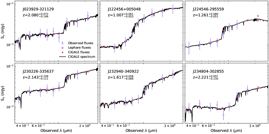
Figure 3: The SED fitting results from Lephare and Cigale for the 6 source galaxies. In each panel, we show the observed multi-band flux from the lensing model (Purple circles with error bars), the template flux from Lephare (blue squares), and the template spectrum from Cigale (black solid line) and its corresponding template flux (red dots). The 4000 $\rm\AA$ break can be clearly seen in the spectra and the template flux, and their locations are consistent with the fitted photo-$z$s.

3.2 Photo-zs and stellar population parameters of the sources from SED fitting

Source redshifts are essential for two main reasons: 1) to confirm the high-$z$ nature of the multiple images and 2) to convert the angular sizes in arcsec into the physical scales in kpc to be used for the scaling relations. As we have spectroscopic redshifts for two systems only, we use the SED fitting of the 9-band photometry of the sources to determine the photometric redshifts. This approach has been found to be reasonably accurate for normal lenses using optical imaging from ground-based observations (see a.g. Langeroodi et al. 2023). In our case, the unique availability of the NIR and the higher lensing model accuracy allowed by pseudo-cross lensing configurations (Gu et al. 2022), suggesting that we can reach possibly a similar or better accuracy.

The SED fitting is performed with the code Lephare (Ilbert et al. 2006). We use the BC03 (Bruzual & Charlot 2003) stellar population synthesis models, a Chabrier (Chabrier 2003) stellar Initial Mass Function and exponentially decaying star formation history. As we expect these systems to be compact, poorly star-forming, old systems, we assume solar metallicity (as found for previous lensed pBNs in N+20), while all other parameters, such as the e-folding time, age of the main stellar population and internal extinction, E(B-V), are free to vary. For each source in the lens systems, we let the redshift vary in the range of (0, 4), and require Lephare to output the best-fitting parameters, e.g. photo-$z$s, stellar mass, age, SFRs, and the corresponding errors. The resulting photo-$z$s, as well as other stellar population parameters, are shown in Tab. 2. To check the robustness of our photo-$z$ estimates, we verify the consistency of the results from the “flexible” and “frozen” models (see §3.1), and further compare the photo-$z$ and spec-$z$s of the two N+20 spectroscopically confirmed lenses. The comparison between the two models (see also Appendix A) shows that the photo-$z$s from different models are consistent within the typical errors expected for high-$z$ galaxy photo-$z$s from ground-based observations (e.g. van den Busch et al. 2020; Amaro et al. 2021; Li et al. 2022). The flexible result shows that the N+20 objects have photo-$z$s of $1.01_{-0.05}^{+0.06}$ and $1.62_{-0.07}^{+0.06}$, respectively, which are fully consistent with their spec-$z$s of $1.101$ and $1.589$.

The source redshifts of the 6 SL systems cover the redshift range $1.0-2.3$. In Fig. 3 we show the observed fluxes and the best-fitted SED templates for the sources of the 6 SL systems for the “flexible” model only. The best fit of the multi-band photometry is remarkably good in all cases. In particular, the NIR bands are essential to closely map the rest-frame 4000 Å break, which is essential in the photo-$z$ determination.

As a consistency check, to make sure that the parameters obtained by Lephare are tool-independent, we repeat the same analysis with Cigale (v2018.0, Boquien et al. 2019). Since this latter is not designed to predict photo-$z$s, we fix the redshift of each source to the photo-$z$s from Lephare. The resulting stellar mass, age, and SFRs of the sources (see Tab. 2) are consistent with Lephare estimates, except for KiDSJ023929$-$321129, whose source turns out to be more massive and old, with a lower $\rm log(sSFRs)$ more compatible with those inferred for the other five systems. As Cigale does not provide uncertainties on the best-estimated parameters, we will use Lephare results as a reference for stellar population parameters in the following. We finally remark that all stellar population estimates are also consistent with the ones obtained with the “frozen” model magnitudes, within the typical statistical errors of stellar populations, as discussed in Appendix A.

Finally, in Table 2, we report the deflector photo-$z$s, that have been derived following the same procedure for the source photo-$z$. The details of this part of the analysis are beyond the purpose of this paper and will be the focus of an upcoming ray-tracing analysis (Li et al., in preparation). Here we just remark that all the systems are consistent with being lensing events, as the redshift of the central galaxy is lower than the one of the background source. The photo-$z$ of the two spectroscopic systems from N+20 are $0.31_{-0.08}^{+0.22}$ and $0.63_{-0.07}^{+0.09}$, slightly higher than their spec-$z$s of $0.237$ and $0.381$, but consistent within $\sim 2\sigma$ in the worse case, which is rather acceptable for reasonably accurate photometric redshifts.

4 Results and Discussion

In this section we concentrate on the results obtained with the flexible model, while the ones from the frozen approach are discussed in Appendix A. We start by using the photo-$z$ derived in Table 2 to convert the effective radii $R_{\rm eff}$ into the physical scale. We find that all sources have $R_{\rm eff}$ smaller than 1.5 kpc, while stellar masses are in the range of $9.9<\log(M_{*}/M_{\odot})<10.5$, as reported in Tab. 2. In the same table, the surface mass densities within 1 kpc are listed and are larger than $\log(\Sigma_{1}/M_{\odot}\rm kpc^{2})\sim 9.3$. These numbers make these sources consistent with typical parameters of blue nuggets (e.g., Zolotov et al. 2015, Tacchella et al. 2016, Barro et al. 2017). The ages of these galaxies are generally older than 1.0 Gyr, except for J023929-321129, which has an age of only 0.5 Gyrs. The two N+20 systems remain the oldest ones in the sample with the new SL-based 9-band photometry showing ages of 3 and 4.5 Gyr, i.e. less than 25% larger than previously found in N+20. All systems show low specific star formation rates, i.e. $\log\rm(sSFR)\lesssim 0.4\ M_{\odot}Gyr^{-1}$, which are consistent with the definition of quiescent systems (see Johnston et al. 2015a, Zolotov et al. 2015, Barro et al. 2017, Huertas-Company et al. 2018). In conclusion, in line with the findings presented in N+20, these systems are all fully compatible with being pBNs.

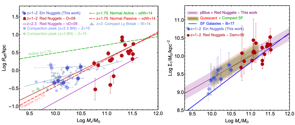
Figure 4: Left: size-mass relation of the pBNs (blue dots) and other galaxies from literature, i.e., 1) red nuggets at $1<z<2$ and their linear fit (red dots and red solid line, Damjanov et al. 2009), and linear fit to the red nuggets at $z\sim 2.3$ (purple line, van Dokkum et al. 2008; 2) the compaction peak of blue nuggets at $z<2.5$ (green squares) and $z>3$ (blue squares) in simulations (Zolotov et al. 2015); 3) the compact LBGs at $z\sim 3$ and their linear fit (blue crosses and blue solid line); 4) linear fit to the measurements of normal passive (red dash lines) and active (green dash lines) galaxies at $z=$1.75 (van der Wel et al. 2014). All of the masses have been corrected to Chabriar-IMF. Right: $\Sigma_{1}$-mass relation of the pBNs (blue dots) and red nuggets (red dots) at $1<z<2$ from Damjanov et al. (2009)). The solid green line is the best-fit relation, while the green dashed lines represent the $1\sigma$ error of the fitted relation. In both plots, it is clear that the pBNs follow the trend of the passive galaxies and Red Nuggets, rather than standard active galaxies at the same redshift.

Further support for this conclusion comes from other similar results obtained in literature: 1) in terms of the $\rm log(SFR)$–mass relation, Johnston et al. (2015b, see their Fig. 6) show that for galaxies with masses of $\rm 9.9\lesssim log(M/M_{\odot})\lesssim 10.5$, the transition place between star-forming galaxies and passive galaxies occurs at $\rm 0.5\lesssim log(SFR/Gyr^{-1})\lesssim 1.5$, compatible to what found for our pBN sample, $\rm 0.2\lesssim log(SFR/Gyr^{-1})\lesssim 1.6$; 2) in terms of the $\rm log(sSFR)$–$\rm log(\Sigma_{1})$ relation, Huertas-Company et al. (2018) shows that the pBNs at $1.4<z<2.2$, and with a central mass density of $\rm log(\Sigma_{1})\leavevmode\nobreak\ \hbox to0.0pt{$>$\hss}{\lower 4.30554pt\hbox{$\sim$}}9.0$ $\rm M_{\odot}$, have $\rm-1.5\lesssim log(sSFR/Gyr)\lesssim 0$. This latter study also shows that the density of pBNs in the above mass and redshift ranges is higher than the density of blue nuggets. For this reason, and for the “selection effect” from the faint NIR photometry, making us little sensitive to strong star-forming systems at $z>1$, as discussed in §2, we tend to select blue (due to the depth in optical bands), compact (due to the strong lensing effect), low star-forming systems, all conspiring toward a selection of pBNs.

The size-mass relation for the 6 pBNs is plotted in the left panel of Fig. 4 (blue solid circles). Here, we also show: 1) red nuggets at $z\sim 1.5$ from Damjanov et al. (2009) (red solid circles and best fit linear line) and at $z\sim 2.3$ from van Dokkum et al. (2008) (purple solid line); 2) compact Ly$\alpha$ break galaxies (LBGs) at $z\sim 3$ from Williams et al. (2014) (blue crosses); 3) normal active galaxies (green dash lines) and passive galaxies (red dash lines) at z=1.75 from van der Wel et al. (2014). All stellar masses are corrected to a Chabrier-IMF, consistently with our choice. From Fig. 4, we see that our lensed pBNs are located away from the size-mass relationship of the star-forming galaxies (green dashed line). Rather, they mainly occupy the location of the compaction peak of blue nuggets at $z<2.5$ (blue boxes) and $z>3$ (green boxes) predicted by simulations (Zolotov et al. 2015). This shows that the typical masses and sizes of the 6 systems are fully compatible with post-compacted galaxies. The log-linear mass-size relation for the pBNs and red nuggets, $\rm logR_{\rm eff}=\alpha log(M_{*})$, gives a slope $\alpha\sim 0.66$. Compared to “red nuggets” and passive galaxies at similar redshift ($z=1.5$ and $z=1.75$ respectively), the lensed pBNs are generally aligned to the size-mass relations of both samples, while they all seem offset by $\sim 0.5$dex with respect to the red nugget samples at $2<z<3$ ($\alpha\sim 0.3$, van Dokkum et al. 2008), possibly due to the earlier formation of these higher-$z$ systems. Finally, the pBN sample looks aligned to the compact Lyman break galaxies (blue crosses), which are believed to be blue nuggets with strong star formation ($\rm log(sSFR)>0.5$ or $\rm log(SFR)>3$, Williams et al. 2014), however, the slope of these latter is $0.38$ (light blue line in Fig. 4), slightly flatter than that of the pBNs plus red nuggets. This confirms the scenario that pBNs share properties of both active and passive compact galaxies, because the quenching occurs after compaction in the post-BN phase and the 6 pBN systems seems indeed in the transition from typical “blue nugget” systems to the “red nuggets”. The turning knee of the two size-mass relationships appears at the location of $\rm log(M_{*}/M_{\odot})\sim$10-10.5. This has been indicated as a characteristic mass scale for a structural transition of the red-blue nugget systems (see e.g. Lapiner et al. 2023), mainly because of the dominance of the wet processes (gas inflows) at lower mass scales, and the dry processes (e.g. dry mergers) acting at larger mass scales. Finally, in the same Fig. 4, we show, as lighter blue data, the results of the frozen model for comparison. We see that two of the systems deviates from the $R_{\rm eff}-M_{*}$ relation. If we take their $\rm\log SFR$s at face value (see Appendix A), these two systems turn out to be very close or superior to the upper SFRs limits discussed in literature (e.g. Johnston et al. 2015b, Huertas-Company et al. 2018, see above). This leave us with the possibility that 2 of the 6 systems are still in the transition to the BN phase, as also suggested by their $\Sigma_{1}$ (see below).

On the right panel of Fig. 4, we show the density inside 1 kpc vs. stellar mass of the pBN. Here, the alignment with red nuggets is even more evident than the size-mass relation on the left panel. The log-linear relation gives a slope of 0.65, fully consistent with the one found for the quiescent galaxies in the redshift range $1.4<z<2$ by Barro et al. (2017, also reported in Fig. 4 – right). This latter work also shows that the compact star forming galaxies (SFGs) follow the sequence of the quiescent galaxies, consistently with the scenario that compaction produces a fast core growth causing normal SFGs to move up from the main SFG sequence (see blue line reported in Fig. 4 – right). In this respect, the two frozen models outliers seen above, occupy the region of the transition from the star forming systems to compact SFGs, suggesting that they might even still going through compaction. This indicates that the classification of these two systems as pBNs is the most insicure one and they might therefore need a spectroscopic follow-up.

5 conclusions

We have collected 6 strong gravitational lens systems with blue point-like lensed images from the catalog of “high-quality candidates” from the Kilo Degree Survey (Li et al. 2021). We have performed ray-tracing modelling in the 9-band imaging data and derived the intrinsic multi-band photometry of the sources. Via photo-$z$ and stellar population analysis, we have confirmed that 1) the systems are genuine SL events; and 2) the background sources of these 6 SL systems are very likely post-blue nuggets (pBNs) because of their very small effective radii, large mass, and low star formation rate, although, 3) depending on the priors on the ray-tracing model (i.e. whether one leave almost multi-band parameters free or fixed to the highest quality $r$-band model), there is a possibility that 2 of the 6 systems are still in a transition phase. In particular, from the perspective of the $\rm log(SFR)$–mass and $\rm log(sSFR)$–$\rm log(\Sigma_{1})$ relations, the 6 pBNs are well consistent with observations of compact low sSFRs objects in Johnston et al. (2015b) and Huertas-Company et al. (2018). In terms of the size-mass and $\Sigma_{1}$-mass relations, these pBNs do not follow the main sequence of star-forming galaxies but align well with the relation of the passive, compact red nuggets at similar redshifts. Also, they sit on the tail of the size mass relation of the compact Ly-Break galaxies (LBGs) from Williams et al. (2014). However, the two systems showing up as outlier in the frozen priors’ model, taken at face value, possess a SFR which is compatible with ongoing star formation and occupy the region of these scaling relations of transient objects from normal star forming galaxies to the post-BN systems. Overall, considering the continuity of the size-mass relations of the compact SFGs and the red nuggets, the “confirmed” pBNs (especially looking at the flexible prior results) sit in a knee located at $\log M_{*}/M_{\odot}\sim 10.5$ consistently with the presence of a characteristic mass for wet compaction (Lapiner et al. 2023).

All these facts together indicate that the pBNs are in a transition phase between the blue and red nuggets, as all structural scaling relations are set to become red nuggets, but with some residual ongoing star formation. This latter is seen, for the two systems in Napolitano et al. (2020), from weak emission lines coexisting however with stellar absorption lines typical of old stellar populations. Finally, taking the modeled Sérsic indexes of these 6 pBNs at face value, regardless of the adopted prior, they are generally smaller ($n<3$) than the predictions from simulations ($n>3$) or observations of red nuggets (Damjanov et al. 2009). Nevertheless, these values are compatible with the scenario that, during the pBN phase, i.e. after the gas is depleted from the centre leaving behind a compact passive nugget, a new extended rotation-supported gas disc/ring can develop (Toft et al. 2017; Lapiner et al. 2023). The only way to obtain a more detailed model and shed light on this aspect would be to obtain higher quality images.

This work is based on a small number of objects (possibly all we can expect, according to N+20) found in the KiDS footprint, but other candidates have been identified in the footprint of other surveys like HSC (Jaelani et al. 2020) and DES (Jacobs et al. 2019). We plan to extend this analysis to other systems soon, and possibly add spectroscopic data in order to further observationally support the understanding of the pBN phase which is crucial in the morphological transformation of galaxies in their early phase of evolution.

Appendix A Multi-band ray-tracing frozen model results

In this appendix, we report the results of the “frozen” prior model described in §3.1, and compare them with the “flexible” prior results. In Table 3, we report the full multi-band parameters for the “flexible” model in Table 1. We can measure the mean and the standard deviation of the source magnitudes derived from the two models as a measure of the average consistency from the two sets of magnitudes, and find these to be $-0.002\pm 0.2139$. This shows no systematics between the two models and a statistical error consistent with typical photometric errors for ground-based observations. The corresponding photo-$z$ are also compared with the ones from the “flexible” model in the left panel in Fig. 5: these also show a rather large scatter but within the typical uncertainties expected for ground-based photo-$z$s (e.g. van den Busch et al. 2020; Amaro et al. 2021; Li et al. 2022). To assess the impact of the variation on the photo-$z$s, we plot in the middle panel of Fig. 5 the corresponding scatter on the source physical effective radii, Finally, we cumulatively compare the stellar masses and the specific star formation rates in the right panel in Fig. 5. As expected, the mag and photo-$z$ errors propagate more dramatically on the stellar population parameters, especially sSFRs, with a typical deviation of the order or 0.2 dex for stellar masses and 0.3-0.4 dex for sSFRs. These are not dissimilar to typical statistical errors found for stellar population parameters using normal KiDS galaxies (e.g. Xie et al. 2023), although they are big enough to move galaxies above the upper limit assumed to separate compact star-forming systems from compact quenched systems in observations (i.e. $\rm\log sSFR\sim 0M_{\odot}^{-1}$, see again Johnston et al. 2015b and Huertas-Company et al. 2018). However, if we consider the typical errors on sSFRs (marked as a shaded region), all systems are stil compatible with a “quenching” scenario. To be conservative, and considering the typical uncertainties on sSFRs (marked as grey shaded region) and the results of the “frozen” priors at face value, 2 of the 6 systems have both sizes and sSFRs that deviate from the expectation to be pBN (see a more detailed discussion in §4).

Table 3: Source properties from the multi-band ray tracing “frozen” model.

ID	$R_{\rm eff}$	$b/a$	$pa$	n	u	g	r	i	Z	Y	J	H	Ks
	(arcsec)		(deg)		(mag)	(mag)	(mag)	(mag)	(mag)	(mag)	(mag)	(mag)	(mag)
J023929$-$321129	0.051$\pm$0.002	0.48$\pm$0.03	90	2.6$\pm$0.1	23.84	23.46	23.30	23.34	23.29	23.46	23.17	22.73	-
J122456$+$005048*	0.042$\pm$0.002	0.41$\pm$0.02	98	2.0$\pm$0.1	-	23.97	23.52	22.87	22.34	22.13	21.79	21.60	21.47
J224546$-$295559	0.056$\pm$0.005	0.45$\pm$0.06	16	3.4$\pm$0.3	24.10	23.81	23.71	23.75	23.70	23.15	22.57	-	-
J230226$-$335637	0.138$\pm$0.007	0.56$\pm$0.04	68	2.4$\pm$0.3	23.48	23.06	23.08	22.99	22.78	22.73	22.20	22.17	-
J232940$-$340922*	0.077$\pm$0.012	0.29$\pm$0.03	168	1.8 $\pm$0.8	-	23.64	23.44	23.36	23.33	22.69	22.36	22.15	21.87
J234804$-$302855	0.167$\pm$0.008	0.38$\pm$ 0.03	71	1.3$\pm$0.2	23.95	23.64	23.68	23.62	23.94	23.37	22.82	22.70	-

Note. — Column content is as in Table 1.

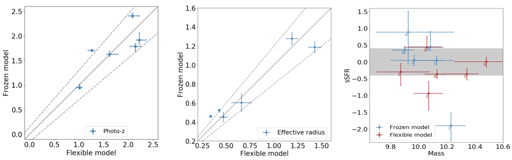
Figure 5: Comparison of relevant parameters obtained from the frozen model and flexible model. Left: photometric redshifts (photo-$z$s). The black solid line represents the 1-to-1 relation of the two photo-$z$s, while the two black dashed lines show the 15 % bias defined as $|\delta z|=|z_{\rm froz}-z_{\rm flex}|/(1+z_{\rm flex})$. Middle: effective radius. The solid line is again the 1-to-1 relation, while the dashed lines represent the 20% bias defined as $|\delta r|=|r_{\rm froz}-r_{\rm flex}|/r_{\rm flex}$. Right: The specific star formation rate (sSFR) versus mass for both the frozen model (blue) and flexible model (red). The solid orizontal line indicate the typical sSFR found for pBNs in CANDELS (Huertas-Company et al. 2018) at redshift $1.4<z<2.0$, while the shaded regions indicate a $\pm 0.4$dex errors, which are realistic statistical errors on sSFRs using 9-band KiDS photometry and photo-$z$ (see Xie et al. 2023). The numbers 1-6 represent the six nuggets in the order listed in Table 1.

References

- Amaro et al. (2021) Amaro, V., Cavuoti, S., Brescia, M., et al. 2021, in Intelligent Astrophysics, ed. I. Zelinka, M. Brescia, & D. Baron, Vol. 39, 245–264, doi: 10.1007/978-3-030-65867-0_11
- Barro et al. (2013) Barro, G., Faber, S. M., Pérez-González, P. G., et al. 2013, ApJ, 765, 104, doi: 10.1088/0004-637X/765/2/104
- Barro et al. (2014) —. 2014, ApJ, 791, 52, doi: 10.1088/0004-637X/791/1/52
- Barro et al. (2017) Barro, G., Faber, S. M., Koo, D. C., et al. 2017, ApJ, 840, 47, doi: 10.3847/1538-4357/aa6b05
- Boquien et al. (2019) Boquien, M., Burgarella, D., Roehlly, Y., et al. 2019, A&A, 622, A103, doi: 10.1051/0004-6361/201834156
- Bruzual & Charlot (2003) Bruzual, G., & Charlot, S. 2003, MNRAS, 344, 1000, doi: 10.1046/j.1365-8711.2003.06897.x
- Cattaneo et al. (2009) Cattaneo, A., Faber, S. M., Binney, J., et al. 2009, Nature, 460, 213, doi: 10.1038/nature08135
- Chabrier (2003) Chabrier, G. 2003, PASP, 115, 763, doi: 10.1086/376392
- Costantin et al. (2021) Costantin, L., Pérez-González, P. G., Méndez-Abreu, J., et al. 2021, ApJ, 913, 125, doi: 10.3847/1538-4357/abef72
- Damjanov et al. (2009) Damjanov, I., McCarthy, P. J., Abraham, R. G., et al. 2009, ApJ, 695, 101, doi: 10.1088/0004-637X/695/1/101
- de Jong et al. (2013) de Jong, J. T. A., Verdoes Kleijn, G. A., Kuijken, K. H., & Valentijn, E. A. 2013, Experimental Astronomy, 35, 25, doi: 10.1007/s10686-012-9306-1
- de Vaucouleurs (1948) de Vaucouleurs, G. 1948, Annales d’Astrophysique, 11, 247
- Dekel & Burkert (2014) Dekel, A., & Burkert, A. 2014, MNRAS, 438, 1870, doi: 10.1093/mnras/stt2331
- Dekel et al. (2009) Dekel, A., Sari, R., & Ceverino, D. 2009, ApJ, 703, 785, doi: 10.1088/0004-637X/703/1/785
- Dekel & Silk (1986) Dekel, A., & Silk, J. 1986, ApJ, 303, 39, doi: 10.1086/164050
- Gu et al. (2022) Gu, A., Huang, X., Sheu, W., et al. 2022, ApJ, 935, 49, doi: 10.3847/1538-4357/ac6de4
- Huertas-Company et al. (2018) Huertas-Company, M., Primack, J. R., Dekel, A., et al. 2018, ApJ, 858, 114, doi: 10.3847/1538-4357/aabfed
- Ilbert et al. (2006) Ilbert, O., Arnouts, S., McCracken, H. J., et al. 2006, A&A, 457, 841, doi: 10.1051/0004-6361:20065138
- Jacobs et al. (2019) Jacobs, C., Collett, T., Glazebrook, K., et al. 2019, ApJS, 243, 17, doi: 10.3847/1538-4365/ab26b6
- Jaelani et al. (2020) Jaelani, A. T., More, A., Sonnenfeld, A., et al. 2020, MNRAS, 494, 3156, doi: 10.1093/mnras/staa583
- Johnston et al. (2015a) Johnston, R., Vaccari, M., Jarvis, M., et al. 2015a, MNRAS, 453, 2540, doi: 10.1093/mnras/stv1715
- Johnston et al. (2015b) —. 2015b, MNRAS, 453, 2540, doi: 10.1093/mnras/stv1715
- Kormann et al. (1994) Kormann, R., Schneider, P., & Bartelmann, M. 1994, A&A, 284, 285
- Kuijken et al. (2019) Kuijken, K., Heymans, C., Dvornik, A., et al. 2019, A&A, 625, A2, doi: 10.1051/0004-6361/201834918
- Langeroodi et al. (2023) Langeroodi, D., Sonnenfeld, A., Hoekstra, H., & Agnello, A. 2023, A&A, 669, A154, doi: 10.1051/0004-6361/202244370
- Lapi et al. (2018) Lapi, A., Pantoni, L., Zanisi, L., et al. 2018, ApJ, 857, 22, doi: 10.3847/1538-4357/aab6af
- Lapiner et al. (2023) Lapiner, S., Dekel, A., Freundlich, J., et al. 2023, arXiv e-prints, arXiv:2302.12234, doi: 10.48550/arXiv.2302.12234
- Li et al. (2020) Li, R., Napolitano, N. R., Tortora, C., et al. 2020, ApJ, 899, 30, doi: 10.3847/1538-4357/ab9dfa
- Li et al. (2021) Li, R., Napolitano, N. R., Spiniello, C., et al. 2021, ApJ, 923, 16, doi: 10.3847/1538-4357/ac2df0
- Li et al. (2022) Li, R., Napolitano, N. R., Feng, H., et al. 2022, A&A, 666, A85, doi: 10.1051/0004-6361/202244081
- Liu et al. (2016) Liu, F. S., Jiang, D., Guo, Y., et al. 2016, ApJ, 822, L25, doi: 10.3847/2041-8205/822/2/L25
- Marques-Chaves et al. (2022) Marques-Chaves, R., Schaerer, D., Álvarez-Márquez, J., et al. 2022, MNRAS, 517, 2972, doi: 10.1093/mnras/stac2893
- Murray et al. (2005) Murray, N., Quataert, E., & Thompson, T. A. 2005, ApJ, 618, 569, doi: 10.1086/426067
- Napolitano et al. (2020) Napolitano, N. R., Li, R., Spiniello, C., et al. 2020, ApJ, 904, L31, doi: 10.3847/2041-8213/abc95b
- Newman et al. (2012) Newman, A. B., Ellis, R. S., Bundy, K., & Treu, T. 2012, ApJ, 746, 162, doi: 10.1088/0004-637X/746/2/162
- Nipoti et al. (2012) Nipoti, C., Treu, T., Leauthaud, A., et al. 2012, MNRAS, 422, 1714, doi: 10.1111/j.1365-2966.2012.20749.x
- Oldham et al. (2017) Oldham, L., Auger, M. W., Fassnacht, C. D., et al. 2017, MNRAS, 465, 3185, doi: 10.1093/mnras/stw2832
- Oser et al. (2012) Oser, L., Naab, T., Ostriker, J. P., & Johansson, P. H. 2012, ApJ, 744, 63, doi: 10.1088/0004-637X/744/1/63
- Petrillo et al. (2019) Petrillo, C. E., Tortora, C., Vernardos, G., et al. 2019, MNRAS, 484, 3879, doi: 10.1093/mnras/stz189
- Posti et al. (2014) Posti, L., Nipoti, C., Stiavelli, M., & Ciotti, L. 2014, MNRAS, 440, 610, doi: 10.1093/mnras/stu301
- Renzini (2006) Renzini, A. 2006, ARA&A, 44, 141, doi: 10.1146/annurev.astro.44.051905.092450
- Sergeyev et al. (2018) Sergeyev, A., Spiniello, C., Khramtsov, V., et al. 2018, Research Notes of the American Astronomical Society, 2, 189, doi: 10.3847/2515-5172/aae6c5
- Sersic (1968) Sersic, J. L. 1968, Atlas de Galaxias Australes
- Spiniello et al. (2021) Spiniello, C., Tortora, C., D’Ago, G., et al. 2021, A&A, 646, A28, doi: 10.1051/0004-6361/202038936
- Tacchella et al. (2016) Tacchella, S., Dekel, A., Carollo, C. M., et al. 2016, MNRAS, 458, 242, doi: 10.1093/mnras/stw303
- Tessore et al. (2016) Tessore, N., Bellagamba, F., & Metcalf, R. B. 2016, MNRAS, 463, 3115, doi: 10.1093/mnras/stw2212
- Toft et al. (2017) Toft, S., Zabl, J., Richard, J., et al. 2017, Nature, 546, 510, doi: 10.1038/nature22388
- Trager & Somerville (2009) Trager, S. C., & Somerville, R. S. 2009, MNRAS, 395, 608, doi: 10.1111/j.1365-2966.2009.14571.x
- van den Busch et al. (2020) van den Busch, J. L., Hildebrandt, H., Wright, A. H., et al. 2020, A&A, 642, A200, doi: 10.1051/0004-6361/202038835
- van der Wel et al. (2014) van der Wel, A., Franx, M., van Dokkum, P. G., et al. 2014, ApJ, 788, 28, doi: 10.1088/0004-637X/788/1/28
- van Dokkum et al. (2008) van Dokkum, P. G., Franx, M., Kriek, M., et al. 2008, ApJ, 677, L5, doi: 10.1086/587874
- Whitaker et al. (2012) Whitaker, K. E., Kriek, M., van Dokkum, P. G., et al. 2012, ApJ, 745, 179, doi: 10.1088/0004-637X/745/2/179
- Williams et al. (2014) Williams, C. C., Giavalisco, M., Cassata, P., et al. 2014, ApJ, 780, 1, doi: 10.1088/0004-637X/780/1/1
- Worthey (1994) Worthey, G. 1994, ApJS, 95, 107, doi: 10.1086/192096
- Xie et al. (2023) Xie, L., Napolitano, N. R., Guo, X., et al. 2023, arXiv e-prints, arXiv:2307.04120, doi: 10.48550/arXiv.2307.04120
- Zolotov et al. (2015) Zolotov, A., Dekel, A., Mandelker, N., et al. 2015, MNRAS, 450, 2327, doi: 10.1093/mnras/stv740