On action ground states of defocusing nonlinear Schrödinger equations

Abstract.

In this work, we study some mathematical features for the action ground states of the defocusing nonlinear Schrödinger equation with possible rotation. Main attention is paid to characterizing the relation between the action ground states and the energy ground states. Theoretical equivalence and non-equivalence results have been established. Asymptotic behaviours of the physical quantities are derived in some limiting parameter regimes. Numerical evidence of non-equivalence is observed and numerical explorations for vortices phenomena in action ground states are done.

Keywords: defocusing nonlinear Schrödinger equation, action ground state, rotation, energy ground state, asymptotics, quantized vortices

AMS Subject Classification: 35B38, 35Q55, 58E30, 81-08

1. Introduction

The following rotating nonlinear Schrödinger equation (RNLS) is widely concerned in physical applications:

$$i\partial_{t}\psi(\mathbf{x},t)=-\frac{1}{2}\Delta\psi(\mathbf{x},t)+V(\mathbf{x})\psi(\mathbf{x},t)+\beta|\psi(\mathbf{x},t)|^{p-1}\psi(\mathbf{x},t)-\Omega L_{z}\psi(\mathbf{x},t),\quad t>0,\ \mathbf{x}\in\mathbb{R}^{d},$$ (1.1)

where $p>1$, $\Omega,\beta\in\mathbb{R}$ are given parameters and $\psi(\mathbf{x},t):\mathbb{R}^{d}\times\mathbb{R}\to\mathbb{C}$ is the wave function with $\mathbf{x}=(x_{1},\ldots,x_{d})^{\top}$ and $d\in\mathbb{N}_{+}$. Moreover, $V(\mathbf{x})$ is a given real-valued potential function and $L_{z}$ is the so-called angular momentum operator:

$$L_{z}=\left\{\begin{aligned} &i(x_{2}\partial_{x_{1}}-x_{1}\partial_{x_{2}}),\quad d\geq 2,\\ &0,\qquad\qquad\qquad\quad\ \ \,d=1,\end{aligned}\right.$$

with $\Omega$ interpreted as the rotating speed. When $\Omega=0$, (1.1) is the classical NLS with an external potential which is the fundamental model in quantum physics and nonlinear optics. When $\Omega\neq 0$ and $d=2,3$, (1.1) serves as the mean-field model for the dynamics of Bose-Einstein condensates in a rotational frame [4, 5, 7, 12]. When $d\geq 3$, $p<\frac{d+2}{d-2}$ is restricted for well-posedness [2, 8]. The parameter $\beta$ describes the strength of nonlinear interaction, with $\beta>0$ for defocusing type interaction and $\beta<0$ for focusing type. Both defocusing and focusing cases are relevant in applications. Under such setup, the mass $m=\|\psi(\cdot,t)\|_{L^{2}}^{2}$ and the energy

$$E(\psi(\cdot,t)):=\frac{1}{2}\|\nabla\psi\|_{L^{2}}^{2}+\int_{\mathbb{R}^{d}}V|\psi|^{2}\mathrm{d}\mathbf{x}+\frac{2\beta}{p+1}\|\psi\|_{L^{p+1}}^{p+1}+L_{\Omega}(\psi)$$ (1.2)

are preserved by (1.1) in time $t$, where $L_{\Omega}(\psi):=-\Omega\int_{\mathbb{R}^{d}}\overline{\psi}(\mathbf{x})L_{z}\psi(\mathbf{x})\mathrm{d}\mathbf{x}$.

As one special solution for dynamics, the standing wave/stationary solution that maintains its shape is of special interest in various important applications. Examples include the solitary impulse in optical communications and the ground or excited states in cold atoms. With a prescribed frequency $\omega\in\mathbb{R}$ ($-\omega$ referred as chemical potential in quantum physics), the standing wave solution in Equation 1.1 reads $\psi(\mathbf{x},t)=\mathrm{e}^{i\omega t}\phi(\mathbf{x})$, where $\phi$ solves the stationary RNLS:

$$H(\phi):=-\frac{1}{2}\Delta\phi+V\phi+\beta|\phi|^{p-1}\phi-\Omega L_{z}\phi+\omega\phi=0,\quad\phi\neq 0.$$ (1.3)

The fact that Equation 1.3 can admit infinitely many solutions [9, 24] motivates different mathematical ways to define the physically relevant ones among all the nontrivial solutions. In this work, we are concerned with the so-called action ground state that minimizes the action functional:

$$S_{\Omega,\omega}(\phi):=E(\phi)+\omega\|\phi\|_{L^{2}}^{2}=\frac{1}{2}\|\nabla\phi\|_{L^{2}}^{2}+\int_{\mathbb{R}^{d}}V|\phi|^{2}\mathrm{d}\mathbf{x}+\frac{2\beta}{p+1}\|\phi\|_{L^{p+1}}^{p+1}+L_{\Omega}(\phi)+\omega\|\phi\|_{L^{2}}^{2}.$$ (1.4)

That is to say, we are interested in the solution:

$$\phi_{g}\in\mathcal{A}_{\Omega,\omega}:=\arg\min\{S_{\Omega,\omega}(\phi)\ :\ \phi\neq 0,\ H(\phi)=0\}.$$ (1.5)

Such definition of ground states, as far as we know, can date back to the early work of Berestycki and Lions [8], and it has been further developed in subsequent mathematical research, e.g., [1, 13, 14, 15, 23, 26]. However, the studies in the literature mainly concerned the action ground state in case of focusing nonlinearity, while the defocusing case is barely addressed. We mention our recent work [19] concerning the defocusing case of (1.3), where an equivalent unconstrained variational formulation has been identified and the existence of the action ground state has been established with efficient numerical algorithms proposed to compute the ground state solution. Many more mathematical aspects of the defocusing action ground states are still awaiting investigation, and this constitutes one of the goals of our work.

As a matter of fact, a more ‘popular’ definition of ground state in the literature is introduced as the minimization of the energy functional $E$ under a prescribed mass $m>0$ [3, 4, 7, 25]:

$$\phi_{m}^{E}\in\mathcal{B}_{\Omega,m}:=\arg\min\{E(\phi)\ :\ \|\phi\|_{L^{2}}^{2}=m,\ E(\phi)<\infty\},$$ (1.6)

which is referred as the energy ground state. The prescription of mass is preferred among physicists, and so the energy ground states have received extensive investigations in the past two decades. See [4, 10, 18, 25] and the references therein. Note that $\phi_{m}^{E}$ is also a stationary solution satisfying (1.3), and the corresponding chemical potential, playing the role of Lagrange multiplier, is determined as

$$\omega(\phi_{m}^{E})=-\mu(\phi_{m}^{E}),$$

where

$$\mu(\phi): =\frac{1}{\|\phi\|_{L^{2}}^{2}}\bigg{[}\frac{1}{2}\|\nabla\phi\|_{L^{2}}^{2}+\int_{\mathbb{R}^{d}}V|\phi|^{2}\mathrm{d}\mathbf{x}+\beta\|\phi\|_{L^{p+1}}^{p+1}+L_{\Omega}(\phi)\bigg{]}$$

$$=\frac{1}{\|\phi\|_{L^{2}}^{2}}\bigg{[}E(\phi)+\frac{p-1}{p+1}\beta\|\phi\|_{L^{p+1}}^{p+1}\bigg{]}.$$ (1.7)

A long-standing question pertains to the relationship between the action ground state and the energy ground state. More interestingly, it raises the question of if the following diagram can commute:

$$\begin{array}[]{rcccl}\omega&\longrightarrow&\eqref{phi_g-def}&\longrightarrow&\phi_{g}\\[4.30554pt] -\mu(\phi_{m}^{E})\quad\rotatebox[origin={c}]{90.0}{$\displaystyle\dashrightarrow$}{}{}{}{}{}{}&&&&~{}~{}~{}~{}~{}~{}\rotatebox[origin={c}]{-90.0}{$\displaystyle\dashrightarrow$}\quad\|\phi_{g}\|_{L^{2}}^{2}\\[4.30554pt] \phi_{m}^{E}&\longleftarrow&\eqref{energyGS-def}&\longleftarrow&m\\ \end{array}$$ (1.11)

Recently, some numerical investigations have been presented in [19, 26], and some theoretical answers have been provided in [11, 20] for the focusing and non-rotating case ($\beta<0,\Omega=0$) of (1.1).

This paper focuses on the defocusing case of RNLS ($\beta>0$ afterwards) and aims to study some mathematical properties of the action ground state (1.5). We shall analyze to give the asymptotic behaviours of the ground state mass $\|\phi_{g}\|_{L^{2}}$ and action $S_{\Omega,\omega}(\phi_{g})$ with respect to the parameters $\omega$ and $\Omega$ in some limit regimes. Numerical experiments will be done towards finding the critical rotating speed $\Omega^{c}$ for generating the vortex phenomenon in action ground states and understanding how $\Omega^{c}$ is influenced by $\omega$. Our primary objective and efforts are devoted to analyzing the connection between the action ground state and the energy ground state. With the help of the unconstrained minimization characterization from [19], we shall prove that an action ground state is always an energy ground state. The reverse statement, however, turns out to be more complicated, and the rotating case ($\Omega\neq 0$) is significantly different from the non-rotating case ($\Omega=0$).

For the non-rotating case, by using the uniqueness of non-negative action ground state and energy ground state, we can establish a complete equivalence between the two. The diagram (1.11) in this case forms a closed loop. For the rotating case, the absence of uniqueness results for ground states poses a much greater challenge in determining if an energy ground state is also an action ground state. Firstly, we shall provide a conditional equivalence to show that whenever $m>0$ is the mass of some action ground state, then all energy ground states with the mass $m$ share the same chemical potential and must be action ground states. Then, we shall give a sufficient and necessary condition to characterize when the non-equivalence would occur, following largely the framework of arguments in [11]. Although such characterization cannot prove or disprove the equivalence, it suggests numerical experiments where strong evidence of non-equivalence is observed.

The rest of the paper is structured as follows. Some preliminaries for analysis will be given in Section 2. The complete equivalence in the non-rotating case will be established in Section 3. Then, the general rotating case will be studied in Section 4, where the conditional equivalence and non-equivalent situations as well as some asymptotic results are theoretically characterized. Finally, numerical explorations are done in Section 5 and some concluding remarks are made in Section 6.

2. Preliminary

In this section, we present some basic notations, setups and facts and review some useful results that will be called for investigations later.

2.1. Setup and assumption

We assume $V(\mathbf{x})\geq 0$ throughout this paper and introduce the functional spaces

$$L_{V}^{2}(\mathbb{R}^{d}):=\left\{\phi\ :\ \int_{\mathbb{R}^{d}}V(\mathbf{x})|\phi(\mathbf{x})|^{2}\mathrm{d}\mathbf{x}<\infty\right\},\quad X:=H^{1}(\mathbb{R}^{d})\cap L_{V}^{2}(\mathbb{R}^{d}).$$

Clearly, $X$ equipped with the following inner product is a Hilbert space:

$$(u,v)_{X}:=\int_{\mathbb{R}^{d}}\Big{(}\nabla u(\mathbf{x})\cdot\nabla\overline{v(\mathbf{x})}+\big{(}1+V(\mathbf{x})\big{)}u(\mathbf{x})\overline{v(\mathbf{x})}\Big{)}\mathrm{d}\mathbf{x},\quad\forall\ u,v\in X.$$

As stated below, we further assume that $V$ is confining to obtain compact embeddings.

Lemma 2.1 (Compact embedding [4]).

Assume that $V(\mathbf{x})\geq 0\;(\forall\ \mathbf{x}\in\mathbb{R}^{d})$ satisfies the confining condition $\lim_{|\mathbf{x}|\to\infty}V(\mathbf{x})=\infty$. Then the embedding $X\hookrightarrow L^{q}(\mathbb{R}^{d})$ is compact, where $q\in[2,\infty]$ for $d=1$, $q\in[2,\infty)$ for $d=2$, and $q\in[2,2d/(d-2))$ for $d\geq 3$.

By integration by parts, one sees that the angular momentum $L_{\Omega}(\phi)=-\Omega\int_{\mathbb{R}^{d}}\overline{\phi(\mathbf{x})}L_{z}\phi(\mathbf{x})\mathrm{d}\mathbf{x}$ is always real-valued, and $L_{\Omega}(\phi)=0$ for all real-valued $\phi\in X$. Moreover, as a direct conclusion from Young’s inequality, the rotational term can be controlled as follows: when $d\geq 2$, for any constant $\delta>0$,

$$\left|\Omega\int_{\mathbb{R}^{d}}\overline{\phi}L_{z}\phi\,\mathrm{d}\mathbf{x}\right|\leq\int_{\mathbb{R}^{d}}\left(\frac{\delta}{2}|\nabla\phi|^{2}+\frac{|\Omega|^{2}}{2\delta}(x_{1}^{2}+x_{2}^{2})|\phi|^{2}\right)\mathrm{d}\mathbf{x}.$$ (2.1)

Now we state the basic assumptions for our problem which will be assumed in the rest of this paper.

Assumption 2.2.

Let $1<p<\frac{d+2}{d-2}$ for $d\geq 3$ and $1<p<\infty$ for $d=1,2$. Assume that $V(\mathbf{x})\geq 0$, $\lim_{|\mathbf{x}|\to\infty}V(\mathbf{x})=\infty$ and $\Omega$ satisfies either $\Omega=0$ (non-rotating case) or $0<|\Omega|<\Omega_{\max}$ (rotating case), where

$$\Omega_{\max}:=\sup\left\{\gamma>0:\lim_{|\mathbf{x}|\to\infty}\left(V(\mathbf{x})-\frac{\gamma^{2}}{2}(x_{1}^{2}+x_{2}^{2})\right)=\infty\right\}\leq\infty.$$ (2.2)

Under the assumptions above, $S_{\Omega,\omega}$ (1.4) is well-defined on $X$ and the angular momentum can be controlled by $X$-norm as

$$\left|\int_{\mathbb{R}^{d}}\overline{\phi}L_{z}\phi\,\mathrm{d}\mathbf{x}\right|\lesssim\|\phi\|_{X}^{2},$$ (2.3)

where the constant depends exclusively on $V$. In fact, by 2.2, for any $0<\gamma<\Omega_{\text{max}}$, there exists $r_{0}>0$ such that $V(\mathbf{x})\geq\frac{\gamma^{2}}{2}(x_{1}^{2}+x_{2}^{2})$, $|\mathbf{x}|\geq r_{0}$. Then Equation 2.3 follows from

$$\left|\int_{\mathbb{R}^{d}}\overline{\phi}L_{z}\phi\,\mathrm{d}\mathbf{x}\right| \leq\int_{\mathbb{R}^{d}}\left[\frac{1}{2}|\nabla\phi|^{2}+\frac{1}{2}(x_{1}^{2}+x_{2}^{2})|\phi|^{2}\right]\mathrm{d}\mathbf{x}$$

$$=\int_{\mathbb{R}^{d}}\frac{1}{2}|\nabla\phi|^{2}\mathrm{d}\mathbf{x}+\frac{1}{2}\int_{|\mathbf{x}|\geq r_{0}}(x_{1}^{2}+x_{2}^{2})|\phi|^{2}\mathrm{d}\mathbf{x}+\frac{1}{2}\int_{|\mathbf{x}|<r_{0}}(x_{1}^{2}+x_{2}^{2})|\phi|^{2}\mathrm{d}\mathbf{x}$$

$$\leq\int_{\mathbb{R}^{d}}\left[\frac{1}{2}|\nabla\phi|^{2}+\frac{1}{\gamma^{2}}V(\mathbf{x})|\phi|^{2}\right]\mathrm{d}\mathbf{x}+r_{0}^{2}\|\phi\|_{L^{2}}^{2}\lesssim\|\phi\|_{X}^{2}.$$

Our discussions of the parameters can be simplified in the following two means:

• The equation Equation 1.3 enjoys the symmetry $\Omega\leftrightarrow-\Omega$ by taking the complex conjugates. So without loss of generality, we shall assume $\Omega\geq 0$ in the subsequent discussions.

• The given parameter $\beta>0$ in Equation 1.1 and Equation 1.3 certainly affects the value of (1.4) and the minimizer (1.5), but it can be normalized by a simple scaling

  $$S_{\Omega,\omega}(c\phi)=c^{2}\left[\frac{1}{2}\|\nabla\phi\|_{L^{2}}^{2}+\int_{\mathbb{R}^{d}}V|\phi|^{2}d\mathbf{x}+\frac{2}{p+1}\|\phi\|_{L^{p+1}}^{p+1}+L_{\Omega}(\phi)+\omega\|\phi\|_{L^{2}}^{2}\right],$$

  with $c=\beta^{-\frac{1}{p-1}}$. Thus, in the rest of the paper, we shall assume $\beta=1$.

The two parameters $\omega$ and $\Omega$ will decisively affect the features of the ground state, and they will be mainly concerned in our study.

2.2. Related functionals

To study the variational properties of the problem, it is convenient to introduce some more functionals that are closely related to the action. Recall that we have assumed $\beta=1$.

1. Quadratic functional: By excluding the $L^{p+1}$-term in the action $S_{\Omega,\omega}$ (1.4), a quadratic functional is defined as

   $$Q_{\Omega,\omega}(\phi):=\int_{\mathbb{R}^{d}}\left(\frac{1}{2}|\nabla\phi|^{2}+V|\phi|^{2}+\omega|\phi|^{2}-\Omega\overline{\phi}L_{z}\phi\right)\mathrm{d}\mathbf{x}=S_{\Omega,\omega}(\phi)-\frac{2}{p+1}\|\phi\|_{L^{p+1}}^{p+1},\quad\phi\in X.$$

2. Nehari functional: The Nehari functional reads

   $$K_{\Omega,\omega}(\phi):=Q_{\Omega,\omega}(\phi)+\|\phi\|_{L^{p+1}}^{p+1}=S_{\Omega,\omega}(\phi)+\frac{p-1}{p+1}\|\phi\|_{L^{p+1}}^{p+1},\quad\phi\in X$$ (2.4)

   and it induces the Nehari manifold $\mathcal{M}:=\{\phi\in X\backslash\{0\}\ :\ K_{\Omega,\omega}(\phi)=0\}.$

It is known [1, 13] that, the action ground state (1.5) can be equivalently written as the minimizer of (1.4) on the Nehari manifold $\mathcal{M}$, i.e., $\phi_{g}\in\mathcal{A}_{\Omega,\omega}\Leftrightarrow\phi_{g}\in\arg\min\{S_{\Omega,\omega}(\phi)\ :\ \phi\in\mathcal{M}\}$. Moreover, as one key property for the defocusing action ground state, another equivalent variational characterization of the action ground state as an unconstrained action minimizer on $X$ was established in [19], i.e., $\phi_{g}\in\mathcal{A}_{\Omega,\omega}\Leftrightarrow\phi_{g}\in\arg\min\{S_{\Omega,\omega}(\phi)\ :\ \phi\in X\}$. In fact, our analysis of the action ground states will be mainly based on this new variational characterization, and we shall recall it in the following.

Let $R:=-\frac{1}{2}\Delta+V-\Omega L_{z}$ be the linear Schrödinger operator with rotation with $\lambda_{0}(\Omega)$ the smallest eigenvalue of $R$ on $X$, i.e.,

$$\lambda_{0}(\Omega):=\inf_{0\neq\phi\in X}\frac{\int_{\mathbb{R}^{d}}\left(\frac{1}{2}|\nabla\phi|^{2}+V|\phi|^{2}-\Omega\overline{\phi}L_{z}\phi\right)\mathrm{d}\mathbf{x}}{\|\phi\|_{L^{2}}^{2}}.$$ (2.5)

Proposition 2.3 (Unconstrained minimization [19]).

Let $\omega<-\lambda_{0}(\Omega)$. Under Assumption 2.2, there exists a $\phi_{g}\in X$ such that

$$S_{\Omega,\omega}(\phi_{g})=\inf_{\phi\in X}S_{\Omega,\omega}(\phi)=\inf_{\phi\in\mathcal{M}}S_{\Omega,\omega}(\phi)<0,$$ (2.6)

with $\mathcal{M}$ the Nehari manifold. Moreover, there exists some constant $M>0$ depending on $d,p,V,\Omega,\omega$ such that

$$\|\phi\|_{X}\leq M,\quad\forall\phi\in\{\phi\in X\ :\ S_{\Omega,\omega}(\phi)\leq 0\}.$$ (2.7)

Remark 2.4.

The assumption for the potential function $V$ in Proposition 2.3 is a bit more general than that in [19], where the proof remains essentially the same with subtle modifications. Such generalized assumption here allows us to cover more practical cases such as the harmonic-plus-lattice potential of the form $V(\mathbf{x})=\sum_{j=1}^{d}\big{(}\frac{1}{2}\gamma_{j}^{2}x_{j}^{2}+\kappa\sin^{2}(\pi x_{j}/2)\big{)}$ and the harmonic-plus-quartic potential of the form $V(\mathbf{x})=\frac{c_{1}}{4}(|\mathbf{x}|^{2}-c_{2})^{2}$, where $\kappa,c_{1},c_{2}>0$.

In the rest of this paper, we denote the action ground state $\phi_{g}$ as $\phi_{\Omega,\omega}$ to more clearly show its dependence on $\omega$ and $\Omega$. For the non-rotating case (i.e., $\Omega=0$), we adopt the following simplified notations by dropping $\Omega$ dependence:

$$S_{\omega}=S_{0,\omega},\quad Q_{\omega}=Q_{0,\omega},\quad K_{\omega}=K_{0,\omega},\quad\phi_{\omega}=\phi_{0,\omega},\quad\mathcal{A}_{\omega}=\mathcal{A}_{0,\omega},\quad\mathcal{B}_{m}=\mathcal{B}_{0,m}.$$ (2.8)

Also, we abbreviate $\lambda_{0}(\Omega)$ with $\Omega=0$ as $\omega_{0}$:

$$\omega_{0}:=\lambda_{0}(0)=\inf_{0\neq\phi\in X}\frac{\int_{\mathbb{R}^{d}}\left(\frac{1}{2}|\nabla\phi|^{2}+V|\phi|^{2}\right)\mathrm{d}\mathbf{x}}{\|\phi\|_{L^{2}}^{2}}>0.$$ (2.9)

3. Non-rotating case

In this section, we consider the non-rotating case (i.e., $\Omega=0$ in Equation 1.1) to investigate the properties of the action ground states. Particularly, we aim to understand the relation between the energy ground state and the action ground state:

$$\phi_{m}^{E}\in\mathcal{B}_{m}=\arg\min_{\begin{subarray}{c}\phi\in X\\ \|\phi\|_{L^{2}}^{2}=m>0\end{subarray}}E(\phi),\qquad\phi_{\omega}\in\mathcal{A}_{\omega}=\arg\min_{\phi\in X}S_{\omega}(\phi).$$

Simplified notations Equations 2.8 and 2.9 are adopted throughout this section.

3.1. Action ground states are energy ground states

Theorem 3.1.

For any $\omega<-\omega_{0}$, an action ground state $\phi_{\omega}$ associated with $\omega$ is also an energy ground state with mass $m=\|\phi_{\omega}\|_{L^{2}}^{2}$.

Proof.

By Proposition 2.3, the action ground state $\phi_{\omega}$ is a global minimizer of $S_{\omega}$ in $X$, which implies

$$S_{\omega}(\phi_{\omega})=\inf_{\phi\in X}S_{\omega}(\phi)\leq\inf_{\begin{subarray}{c}\phi\in X\\ \|\phi\|_{L^{2}}^{2}=m\end{subarray}}S_{\omega}(\phi).$$

On the other hand,

$$S_{\omega}(\phi_{\omega})=S_{\omega}\left(\frac{\sqrt{m}}{\|\phi_{\omega}\|_{L^{2}}}\phi_{\omega}\right)\geq\inf_{0\neq\phi\in X}S_{\omega}\left(\frac{\sqrt{m}}{\|\phi\|_{L^{2}}}\phi\right)=\inf_{\begin{subarray}{c}\phi\in X\\ \|\phi\|_{L^{2}}^{2}=m\end{subarray}}S_{\omega}(\phi).$$

Noting that, under the constraint $\|\phi\|_{L^{2}}^{2}=m$, there holds the relation $S_{\omega}(\phi)=E(\phi)+\omega m$, one finds

$$\omega m+E(\phi_{\omega})=S_{\omega}(\phi_{\omega})=\inf_{\begin{subarray}{c}\phi\in X\\ \|\phi\|_{L^{2}}^{2}=m\end{subarray}}S_{\omega}(\phi)=\omega m+\inf_{\begin{subarray}{c}\phi\in X\\ \|\phi\|_{L^{2}}^{2}=m\end{subarray}}E(\phi),$$

and therefore,

$$E(\phi_{\omega})=\inf_{\begin{subarray}{c}\phi\in X\\ \|\phi\|_{L^{2}}^{2}=m\end{subarray}}E(\phi),$$

which confirms the assertion. ∎

3.2. Energy ground states are action ground states

Theorem 3.2.

For any $m>0$, an energy ground state $\phi^{E}_{m}$ with mass $m$ is also an action ground state associated with $\omega=-\mu(\phi^{E}_{m})$ where $\mu$ is defined in Section 1 with $\Omega=0$.

The proof will be given with the help of the following lemmas.

Lemma 3.3 (Uniqueness).

For any $\omega<-\omega_{0}$, there exists $\phi_{\omega}\in\mathcal{A}_{\omega}$ satisfying $\phi_{\omega}(\mathbf{x})\geq 0\ (\mathbf{x}\in\mathbb{R}^{d})$ such that

$$|\phi(\mathbf{x})|=\phi_{\omega}(\mathbf{x})\quad\text{\rm a.e. }\mathbf{x}\in\mathbb{R}^{d},\quad\forall\phi\in\mathcal{A}_{\omega}.$$ (3.1)

For any $m>0$, there exists $\phi^{E}_{m}\in\mathcal{B}_{m}$ satisfying $\phi^{E}_{m}(\mathbf{x})\geq 0\ (\mathbf{x}\in\mathbb{R}^{d})$ such that

$$|\phi(\mathbf{x})|=\phi^{E}_{m}(\mathbf{x})\quad\text{\rm a.e. }\mathbf{x}\in\mathbb{R}^{d},\quad\forall\phi\in\mathcal{B}_{m}.$$ (3.2)

Proof.

By the inequality (see [16])

$$\int_{\mathbb{R}^{d}}|\nabla|\phi||^{2}\mathrm{d}\mathbf{x}\leq\int_{\mathbb{R}^{d}}|\nabla\phi|^{2}\mathrm{d}\mathbf{x},\quad\phi\in H^{1}(\mathbb{R}^{d}),$$ (3.3)

recalling Equation 1.4, we get

$$S_{\omega}(|\phi|)\leq S_{\omega}(\phi),\qquad\phi\in X,$$ (3.4)

which implies that, if $\phi$ is an action ground state, $|\phi|$ is also an action ground state. Then Equation 3.1 holds if we have the uniqueness of the nonnegative action ground state or the density.

Consider the density $\rho(\mathbf{x})=|\phi(\mathbf{x})|^{2}\geq 0$ with $\sqrt{\rho}\in X$. Following the process in [17, Lemma A.1], we have $S_{\omega}(\sqrt{\rho})$ is strictly convex with respect to $\rho$, which implies the uniqueness of the density of action ground states and proves Equation 3.1. The proof of Equation 3.2 is similar and can be found in [4, 17]. ∎

Remark 3.4.

In addition to assumptions in Lemma 3.3, if $V\in L^{2}_{\mathrm{loc}}$, then $\phi_{\omega}$ and $\phi^{E}_{m}$ can be chosen as strictly positive, and the action and energy ground states are unique up to a constant phase shift (see [16, 17]).

The proof of Theorem 3.2 will be done by studying the properties of the mass of action ground states as a function of $\omega$, which is well-defined due to the uniqueness result in Lemma 3.3. Define the action ground state mass $M_{g}:(-\infty,-\omega_{0})\rightarrow\mathbb{R}^{+}$ as

$$M_{g}(\omega):=\|\phi_{\omega}\|_{L^{2}}^{2},\quad\omega<-\omega_{0}.$$ (3.5)

In the proof of the following Lemmas 3.5, 3.6 and 3.7, we assume that $\phi_{\omega}$ is the unique nonnegative action ground state associated with $\omega<-\omega_{0}$ and $\phi^{E}_{m}$ is the unique nonnegative energy ground state associated with $m>0$.

Lemma 3.5.

The function $M_{g}$ is injective on $(-\infty,-\omega_{0})$, i.e., for any $\omega_{1},\omega_{2}\in(-\infty,-\omega_{0})$, $M_{g}(\omega_{1})=M_{g}(\omega_{2})$ implies $\omega_{1}=\omega_{2}$.

Proof.

Let $m_{1}=M_{g}(\omega_{1})$ and $m_{2}=M_{g}(\omega_{2})$. By Theorem 3.1, we have $\phi_{\omega_{1}}=\phi^{E}_{m_{1}}$ and $\phi_{\omega_{2}}=\phi^{E}_{m_{2}}$. If $m_{1}=m_{2}$, by the uniqueness of energy ground states in Lemma 3.3, we have $\phi^{E}_{m_{1}}=\phi^{E}_{m_{2}}$ and thus $\phi_{\omega_{1}}=\phi_{\omega_{2}}=:\phi_{\ast}$. Then $\phi_{\ast}$ will solve the stationary NLS

$$-\frac{1}{2}\Delta\phi_{\ast}+V\phi_{\ast}+\omega\phi_{\ast}+|\phi_{\ast}|^{p-1}\phi_{\ast}=0,\quad\omega=\omega_{1},\omega_{2},$$ (3.6)

which implies $\omega_{1}=\omega_{2}$, and completes the proof. ∎

Lemma 3.6.

The function $M_{g}(\omega):=\|\phi_{\omega}\|_{L^{2}}^{2}$ is continuous on $(-\infty,-\omega_{0})$.

Proof.

We first show that $S_{{\omega_{\ast}}}(\phi_{\omega})\to S_{\omega_{\ast}}(\phi_{\omega_{\ast}})$ as $\omega\rightarrow\omega_{\ast}$ for any fixed $\omega_{\ast}\in(-\infty,-\omega_{0})$. Recalling the variational characterization of the action ground states in Equation 2.6 and the expression of the action functional Equation 1.4, we obtain

$$S_{\omega_{\ast}}(\phi_{\omega_{\ast}})<S_{\omega_{\ast}}(\phi_{\omega})<S_{\omega}(\phi_{\omega})<S_{\omega}(\phi_{\omega_{\ast}}), \omega_{\ast}<\omega<-\omega_{0},$$ (3.7)

$$S_{\omega}(\phi_{\omega})<S_{\omega}(\phi_{\omega_{\ast}})<S_{\omega_{\ast}}(\phi_{\omega_{\ast}})<S_{\omega_{\ast}}(\phi_{\omega}), \omega<\omega_{\ast}.$$ (3.8)

For any $\omega_{\ast}<\omega<-\omega_{0}$, by Equation 3.7, we have

$$|S_{\omega_{\ast}}(\phi_{\omega})-S_{\omega_{\ast}}(\phi_{\omega_{\ast}})|<|S_{\omega}(\phi_{\omega_{\ast}})-S_{\omega_{\ast}}(\phi_{\omega_{\ast}})|=|\omega-\omega_{\ast}|M_{g}(\omega_{\ast}).$$ (3.9)

Then, for $\omega<\omega_{\ast}$, by Equation 3.8, we have

$$|S_{\omega_{\ast}}(\phi_{\omega})-S_{\omega_{\ast}}(\phi_{\omega_{\ast}})|<|S_{\omega_{\ast}}(\phi_{\omega})-S_{\omega}(\phi_{\omega})|=|\omega-\omega_{\ast}|M_{g}(\omega).$$ (3.10)

For any fixed $\delta>0$, when $\omega_{\ast}-\delta<\omega<\omega_{\ast}$, by Equations 1.4 and 2.6, we have

$$S_{\omega_{\ast}-\delta}(\phi_{\omega})<S_{\omega}(\phi_{\omega})<0,$$ (3.11)

which implies, by Equation 2.7,

$$M_{g}(\omega)\leq C,\quad\omega_{\ast}-\delta<\omega<\omega_{\ast},$$ (3.12)

where $C$ is some constant depending only on $\omega_{\ast},\delta,d,p,V$. Combing Equations 3.9, 3.10 and 3.12 yields that $S_{\omega_{\ast}}(\phi_{\omega})\to S_{\omega_{\ast}}(\phi_{\omega_{\ast}})$ as $\omega\to\omega_{\ast}$.

As a consequence, for any sequence $\{\omega^{k}\}_{k=1}^{\infty}\subset(-\infty,\omega_{0})$ converging to $\omega_{\ast}$, $\{\phi_{\omega^{k}}\}_{k=1}^{\infty}$ minimizes the functional $S_{\omega_{\ast}}$ in $X$. Hence, by Equations 2.6 and 2.7, $\{\phi_{\omega^{k}}\}_{k=1}^{\infty}$ is uniformly bounded in $X$. Utilizing the same argument used in the proof of [19, Theorem 3.1], we can easily apply the compact embedding given in Lemma 2.1 and the weak lower-semicontinuity of the norm $\|\cdot\|_{X}$ to conclude that $\{\phi_{\omega^{k}}\}_{k=1}^{\infty}$ contains a subsequence converging strongly to the unique nonnegative action ground state $\phi_{\omega_{\ast}}$ in $X$ (and therefore in $L^{2}(\mathbb{R}^{d})$). The arbitrariness of the sequence $\{\omega^{k}\}_{k=1}^{\infty}$ leads to $M_{g}(\omega)=\|\phi_{\omega}\|^{2}_{L^{2}}\to\|\phi_{\omega_{\ast}}\|^{2}_{L^{2}}=M_{g}(\omega_{\ast})$ as $\omega\to\omega_{\ast}$. The proof is completed. ∎

Lemma 3.7 (Limits of mass in $\omega$).

$M_{g}(\omega)\rightarrow 0$ as $\omega\rightarrow{-\omega_{0}}^{-}$ and $M_{g}(\omega)\rightarrow\infty$ as $\omega\rightarrow-\infty$.

Proof.

We first show that $M_{g}(\omega)\rightarrow 0$ as $\omega\rightarrow{-\omega_{0}}^{-}$. By Equation 3.11 with $\omega_{\ast}$ replaced by $-\omega_{0}$, we have $\phi_{\omega}$ is uniformly bounded in $X$ for $\omega\in(-\omega_{0}-\delta,-\omega_{0})$. Recalling Equations 1.4 and 2.9, we have

$$S_{\omega}(\phi_{\omega})\geq(\omega+\omega_{0})\|\phi_{\omega}\|_{L^{2}}^{2}+\frac{2}{p+1}\|\phi_{\omega}\|_{L^{p+1}}^{p+1}\geq(\omega+\omega_{0})\|\phi_{\omega}\|_{L^{2}}^{2},$$ (3.13)

which, together with (2.4) and Equation 2.6, yields

$$0>S_{\omega}(\phi_{\omega})=-\frac{p-1}{p+1}\|\phi_{\omega}\|_{L^{p+1}}^{p+1}\geq(\omega+\omega_{0})\|\phi_{\omega}\|_{L^{2}}^{2}\rightarrow 0\quad\mbox{as}\quad\omega\rightarrow{-\omega_{0}}^{-}.$$ (3.14)

It follows that $\|\phi_{\omega}\|_{L^{p+1}}^{p+1}\rightarrow 0$. To control $\|\phi_{\omega}\|_{L^{2}}$ by $\|\phi_{\omega}\|_{L^{p+1}}^{p+1}$, we claim that for any $A>0$, there exists $r_{0}>0$ such that for $r>r_{0}$, we have

$$\|\phi\|_{L^{2}}^{2}\leq|B_{r}|^{\frac{p-1}{p+1}}\|\phi\|_{L^{p+1}}^{2}+\frac{1}{A}\|\phi\|_{X}^{2},\quad\phi\in X,$$ (3.15)

where $B_{r}=\{\mathbf{x}\in\mathbb{R}^{d}:|\mathbf{x}|<r\}$. In fact, by the confining condition $\lim_{|\mathbf{x}|\rightarrow\infty}V(\mathbf{x})=+\infty$, for any $A>0$, there exists $r_{0}>0$ such that $V(\mathbf{x})+1\geq A$ for any $|\mathbf{x}|\geq r_{0}$. By Hölder’s inequality, for any $r>r_{0}$, we have

$$\|\phi\|_{L^{2}}^{2}=\int_{B_{r}}|\phi|^{2}\mathrm{d}\mathbf{x}+\int_{|\mathbf{x}|\geq r}|\phi|^{2}\mathrm{d}\mathbf{x} \leq|B_{r}|^{\frac{p-1}{p+1}}\|\phi\|_{L^{p+1}}^{2}+\frac{1}{A}\int_{|\mathbf{x}|\geq r}(V(\mathbf{x})+1)|\phi|^{2}\mathrm{d}\mathbf{x}$$

$$\leq|B_{r}|^{\frac{p-1}{p+1}}\|\phi\|_{L^{p+1}}^{2}+\frac{1}{A}\|\phi\|_{X}^{2},$$

which proves the claim Equation 3.15. Since $\phi_{\omega}$ is uniformly bounded in $X$, one has $\|\phi_{\omega}\|_{L^{2}}^{2}\rightarrow 0$ by Equation 3.15.

Then we shall show that $M_{g}(\omega)\rightarrow\infty$ as $\omega\rightarrow-\infty$. Note that for all $\phi\in X$,

$$-\|\phi_{\omega}\|_{L^{2}}^{2}\leq\frac{S_{\omega}(\phi_{\omega})}{|\omega|}\leq\frac{S_{\omega}(\phi)}{|\omega|}=\frac{E(\phi)}{|\omega|}-\|\phi\|_{L^{2}}^{2}.$$

Namely, $M_{g}(\omega)\geq\|\phi\|_{L^{2}}^{2}-\frac{E(\phi)}{|\omega|}$, $\forall\phi\in X$. The arbitrariness of $\phi\in X$ implies that $M_{g}(\omega)\rightarrow\infty$ as $\omega\rightarrow-\infty$. ∎

Proof of Theorem 3.2.

By Lemmas 3.5 and 3.6, we have $M_{g}(\omega)$ is a strictly monotone function on $(-\infty,-\omega_{0})$. Furthermore, by Lemma 3.7, $M_{g}(\omega)$ is strictly decreasing and is surjective from $(-\infty,-\omega_{0})$ to $(0,\infty)$. Hence, for any $m>0$, there exists a unique $\omega$ satisfying $m=M_{g}(\omega)$. Let $\phi_{\omega}$ be an action ground state associated with $\omega$. By Theorem 3.1, we have

$$E(\phi_{\omega})=E(\phi^{E}_{m}),\quad\|\phi_{\omega}\|_{L^{2}}^{2}=\|\phi^{E}_{m}\|_{L^{2}}^{2}=m,$$ (3.16)

which implies

$$S_{\omega}(\phi^{E}_{m})=E(\phi^{E}_{m})+\omega\|\phi^{E}_{m}\|_{L^{2}}^{2}=S_{\omega}(\phi_{\omega}),$$ (3.17)

which further implies that $\phi^{E}_{m}$ is an action ground state associated with $\omega$. That $\omega=-\mu(\phi^{E}_{m})$ follows from noting that $\phi^{E}_{m}$ solves Equation 1.3. ∎

Remark 3.8.

By Equations 3.7 and 3.8, and the analysis in the proof of Lemma 3.6, we also obtain that $S_{g}(\omega):=S_{\omega}(\phi_{\omega})$ is continuous and strictly increasing with respect to $\omega$ on $(-\infty,-\omega_{0})$. Moreover, the proof of Lemma 3.7 implies that

$$\lim_{\omega\rightarrow-\infty}S_{g}(\omega)=-\infty\quad\mbox{and}\quad\lim_{\omega\rightarrow-\omega_{0}^{-}}S_{g}(\omega)=0.$$

In fact, the asymptotics of the limits of mass $M_{g}(\omega)$ and action $S_{g}(\omega)$ in $\omega$ can be derived as well. These will be discussed in the next section that covers the rotating case.

The established Theorems 3.1 and 3.2 together show the complete equivalence of the action ground state and the energy ground state for the non-rotating defocusing NLS. Consequently, mathematical studies for the ground state, such as its stability as a soliton, can be explored in one of the setups.

4. Rotating case

We move on to consider the rotating case, i.e., $\Omega\neq 0$ in (1.1). Again, We shall first focus on the relation between the energy ground state and the action ground state:

$$\phi_{m}^{E}\in\mathcal{B}_{\Omega,m}=\arg\min_{\begin{subarray}{c}\phi\in X\\ \|\phi\|_{L^{2}}^{2}=m>0\end{subarray}}E(\phi),\qquad\phi_{\Omega,\omega}\in\mathcal{A}_{\Omega,\omega}=\arg\min_{\phi\in X}S_{\Omega,\omega}(\phi).$$

Then we shall study some asymptotic limits with respect to $\omega$ and $\Omega$. In this section, we use $\phi_{\Omega,\omega}$ to denote an arbitrary element in $\mathcal{A}_{\Omega,\omega}$.

4.1. Relation with energy ground states

In the case of rotation, there is generally no theoretical guarantee for the uniqueness of the action and/or energy ground state, which becomes the primary difference and difficulty in this context. In fact, if a form of uniqueness for the action ground state (e.g., as shown in Lemma 3.3) is either provided or assumed, the complete equivalence of the two may also be established by following the similar procedure in Section 3. Here, we choose to follow the work of [11], allowing for the possibility of multiple non-trivial action ground states of a given $\omega$.

First of all, Theorem 3.1 can also be extended to the rotating case. That is to say an action ground state $\phi_{\Omega,\omega}$ is certainly an energy ground state with mass $m=\|\phi_{\Omega,\omega}\|_{L^{2}}^{2}$. Moreover, we have the following theorem about the conditional equivalence of the energy ground states and the action ground states. Before stating the theorem, due to the non-uniqueness, we first define the set of mass of action ground states associated with $\omega$ and $\Omega$ as

$$\mathcal{N}_{\Omega,\omega}:=\left\{\|\phi\|_{L^{2}}^{2}:\phi\in\mathcal{A}_{\Omega,\omega}\right\}.$$ (4.1)

Theorem 4.1 (Conditional equivalence).

For any $\omega<-\lambda_{0}(\Omega)$, the action ground state $\phi_{\Omega,\omega}$ is also an energy ground state with mass $m=\|\phi_{\Omega,\omega}\|_{L^{2}}^{2}$, and all the energy ground states $\phi_{m}^{E}$ with precisely this mass $m$ are also action ground states associated with $\omega$. Moreover, we have

$$\mathcal{A}_{\Omega,\omega}=\bigcup_{m\in\mathcal{N}_{\Omega,\omega}}\mathcal{B}_{\Omega,m}.$$ (4.2)

Proof.

Following the proof of Theorem 3.1, we immediately have $\phi_{\Omega,\omega}$ is an energy ground state with mass $m=\|\phi_{\Omega,\omega}\|_{L^{2}}^{2}$. For this $m$, we have $\mathcal{B}_{\Omega,m}\subset\mathcal{A}_{\Omega,\omega}$, which follows from the observation: for any $\phi\in\mathcal{B}_{\Omega,m}$, we have

$$E(\phi)=E(\phi_{\Omega,\omega}),\quad\|\phi\|_{L^{2}}^{2}=m=\|\phi_{\Omega,\omega}\|_{L^{2}}^{2},$$

which implies that $S_{\Omega,\omega}(\phi)=E(\phi)+\omega m=S_{\Omega,\omega}(\phi_{\Omega,\omega})$ and thus $\phi\in\mathcal{A}_{\Omega,\omega}$. As a result, Equation 4.2 follows immediately. ∎

By Theorem 4.1, if the mass of all action ground states as a set can cover $(0,\infty)$, i.e.,

$$\mathcal{N}:=\bigcup_{\omega\in(-\infty,-\lambda_{0}(\Omega))}\mathcal{N}_{\Omega,\omega}=(0,\infty),$$ (4.3)

then an energy ground state $\phi^{E}_{m}$ with any mass $m>0$ is also an action ground state associated with $\omega=-\mu(\phi^{E}_{m})$ with $\mu$ defined in Section 1, and we obtain the complete equivalence of the two. If $\mathcal{N}\neq(0,\infty)$, then for any $m\in(0,\infty)\setminus\mathcal{N}$, the energy ground state with mass $m$ is clearly not an action ground state. Different from the non-rotating case analyzed in Section 3, due to the lack of uniqueness in the rotating case, it is unclear whether Equation 4.3 will hold or not. In the following, instead of proving or disproving Equation 4.3, we shall give a detailed characterization for the set $\mathcal{N}$, which allows us to derive more precise equivalence and non-equivalence conditions.

Similar to the function $M_{g}$ defined in Equation 3.5, we now define

$$m^{\ast}(\omega):=\sup\mathcal{N}_{\Omega,\omega},\qquad m_{\ast}(\omega):=\inf\mathcal{N}_{\Omega,\omega}.$$ (4.4)

As in Section 3.2, we shall study the structure of $\mathcal{N}$ through the properties of two mass functions $m^{\ast}$ and $m_{\ast}$, including continuity, monotonicity and the limit. For ease of presentation, we define another inner product $\langle\cdot,\cdot\rangle_{R(\kappa)}$ on $X$ as

$$\langle\cdot,\cdot\rangle_{R(\kappa)}=\langle R\cdot,\cdot\rangle+\kappa\langle\cdot,\cdot\rangle,\qquad R=-\frac{1}{2}\Delta+V-\Omega L_{z},$$ (4.5)

with $\kappa>\max\{-\lambda_{0}(\Omega),0\}$ a fixed constant. Then, under 2.2, $\|\cdot\|_{R(\kappa)}=\sqrt{Q_{\Omega,\kappa}(\cdot)}$ is an equivalent norm on $X$.

Lemma 4.2.

Let $\omega_{\ast}\in(-\infty,-\lambda_{0}(\Omega))$. For any $\omega^{k}\rightarrow\omega_{\ast}^{+}$ or $\omega^{k}\rightarrow\omega_{\ast}^{-}$, there exist $\phi\in\mathcal{A}_{\Omega,\omega_{\ast}}$ and a subsequence $\{\omega^{n_{k}}\}_{k}$ such that

$$\phi_{\Omega,\omega^{n_{k}}}\rightharpoonup\phi\text{ in }X,\quad\text{ as }k\rightarrow\infty.$$

Proof.

We start with the case $\omega^{k}\rightarrow\omega_{\ast}^{+}$. Note that for any $\omega$ satisfying $\omega_{\ast}<\omega<-\lambda_{0}(\Omega)$, one has, similar to Equation 3.7,

$$S_{\Omega,\omega_{\ast}}(\phi_{\Omega,\omega_{\ast}})<S_{\Omega,\omega_{\ast}}(\phi_{\Omega,\omega})<S_{\Omega,\omega}(\phi_{\Omega,\omega})<S_{\Omega,\omega}(\phi_{\Omega,\omega_{\ast}}).$$ (4.6)

Recalling Equation 1.4, we have

$$S_{\Omega,\omega}(\phi_{\Omega,\omega_{\ast}})\rightarrow S_{\Omega,\omega_{\ast}}(\phi_{\Omega,\omega_{\ast}})\text{\quad as \quad}\omega\rightarrow\omega_{\ast}^{+},$$ (4.7)

which, together with Equation 4.6 yields

$$S_{\Omega,\omega_{\ast}}(\phi_{\Omega,\omega})\rightarrow S_{\Omega,\omega_{\ast}}(\phi_{\Omega,\omega_{\ast}}),$$ (4.8a)

$$S_{\Omega,\omega}(\phi_{\Omega,\omega})\rightarrow S_{\Omega,\omega_{\ast}}(\phi_{\Omega,\omega_{\ast}}).$$ (4.8b)

By Equations 4.8b and 2.4, we have

$$\|\phi_{\Omega,\omega}\|_{L^{p+1}}\rightarrow\|\phi_{\Omega,\omega_{\ast}}\|_{L^{p+1}},\text{\quad as \quad}\omega\rightarrow\omega_{\ast}^{+}.$$

By Equations 4.8a and 2.6, one has $S_{\Omega,\omega_{\ast}}(\phi_{\Omega,\omega})<0$ for $\omega>\omega_{\ast}$ sufficiently close to $\omega_{\ast}$, which implies, by Equation 2.7, $\phi_{\Omega,\omega}$ is uniformly bounded in $X$ for $\omega_{\ast}<\omega<\omega_{\ast}+\delta<-\lambda_{0}(\Omega)$ with some $\delta>0$ sufficiently small. Then, for any sequence $\omega^{k}\rightarrow\omega_{\ast}^{+}$ satisfying $\omega_{\ast}<\omega^{k}<\omega_{\ast}+\delta<-\lambda_{0}(\Omega)$, there exists a subsequence (still denoted by $\{\omega^{k}\}_{k}$) and $\phi\in X$ such that $\phi_{\Omega,\omega^{k}}\rightharpoonup\phi$ weakly in $X$. It remains to show that $\phi\in\mathcal{A}_{\Omega,\omega_{\ast}}$. By Lemma 2.1, $\phi_{\Omega,\omega^{k}}\rightarrow\phi$ strongly in $L^{2}$ and $L^{p+1}$. Recalling Equation 4.5, one has

$$S_{\Omega,\omega_{\ast}}(\phi)=\|\phi\|_{R(\kappa)}^{2}-(\kappa-\omega_{\ast})\|\phi\|_{L^{2}}^{2}+\frac{2}{p+1}\|\phi\|_{L^{p+1}}^{p+1}.$$

Using the weak lower-semicontinuity of the norm $\|\cdot\|_{R(\kappa)}$ in $X$, the strong convergence of $\phi_{\Omega,\omega^{k}}$ in $L^{2}$ and $L^{p+1}$, and Equation 4.8a, we obtain

$$S_{\Omega,\omega_{\ast}}(\phi)\leq\liminf_{k\rightarrow\infty}S_{\Omega,\omega_{\ast}}(\phi_{\Omega,\omega^{k}})=S_{\Omega,\omega_{\ast}}(\phi_{\Omega,\omega_{\ast}}).$$

Hence, $S_{\Omega,\omega_{\ast}}(\phi)=S_{\Omega,\omega_{\ast}}(\phi_{\Omega,\omega_{\ast}})$ and $\phi\in\mathcal{A}_{\Omega,\omega_{\ast}}$.

Then we consider the case $\omega^{k}\rightarrow\omega_{\ast}^{-}$. For any $\omega$ satisfying $\omega<\omega_{\ast}$, one has

$$S_{\Omega,\omega}(\phi_{\Omega,\omega})<S_{\Omega,\omega}(\phi_{\Omega,\omega_{\ast}})<S_{\Omega,\omega_{\ast}}(\phi_{\Omega,\omega_{\ast}})<S_{\Omega,\omega_{\ast}}(\phi_{\Omega,\omega}).$$

We claim that

$$S_{\Omega,\omega_{\ast}}(\phi_{\Omega,\omega})-S_{\Omega,\omega}(\phi_{\Omega,\omega})\rightarrow 0\quad\text{as }\omega\rightarrow\omega_{\ast}^{-}.$$ (4.9)

To show Equation 4.9, it suffices to show that $\|\phi_{\omega}\|_{L^{2}}$ is uniformly bounded when $\omega\rightarrow\omega_{\ast}^{-}$. Note that, for any $\delta>0$,

$$S_{\Omega,\omega_{\ast}-\delta}(\phi_{\Omega,\omega})<S_{\Omega,\omega}(\phi_{\Omega,\omega})<0,\quad\omega_{\ast}-\delta<\omega<\omega_{\ast},$$

which implies by Equation 2.7 that $\{\phi_{\Omega,\omega}\}_{\omega_{\ast}-\delta<\omega<\omega_{\ast}}$ is uniformly bounded in $X$ and thus the claim Equation 4.9 is proved. The rest of the proof follows a similar procedure as in the case $\omega\rightarrow\omega_{\ast}^{+}$ and we shall omit it for brevity. ∎

Now we are able to characterize the mass functions $m^{\ast}$ and $m_{\ast}$ as derivatives of the action function with respect to $\omega$. That is to define $S^{g}_{\Omega}:(-\infty,-\lambda_{0}(\Omega))\rightarrow\mathbb{R}$ as

$$S^{g}_{\Omega}(\omega):=S_{\Omega,\omega}(\phi_{\Omega,\omega}),\quad\omega<-\lambda_{0}(\Omega),$$ (4.10)

and we have the following result for its relation with the mass.

Proposition 4.3.

The left and right derivative of $S^{g}_{\Omega}$ exist everywhere on $(-\infty,-\lambda_{0}(\Omega))$, and we denote them by ${S^{g}_{\Omega}}^{\prime}_{-},{S^{g}_{\Omega}}^{\prime}_{+}$ respectively. Then, we have

$${S^{g}_{\Omega}}^{\prime}_{-}(\omega)=m^{\ast}(\omega),\quad{S^{g}_{\Omega}}^{\prime}_{+}(\omega)=m_{\ast}(\omega),\quad\omega<-\lambda_{0}(\Omega).$$

Proof.

Let $f_{\phi}(\omega)=S_{\Omega,\omega}(\phi)$. Then $f_{\phi}(\cdot)$ is a linear function on $(-\infty,-\lambda_{0}(\Omega))$ for each given $\phi\in X$ and thus is concave. Since

$$S^{g}_{\Omega}(\omega)=\inf_{\phi\in X}S_{\Omega,\omega}(\phi)=\inf_{\phi\in X}f_{\phi}(\omega),$$

$S^{g}_{\Omega}$ is also a concave function on $(-\infty,-\lambda_{0}(\Omega))$ and the one side derivatives exist every where.

For any $\omega_{\ast}<-\lambda_{0}(\Omega)$, we first show that ${S^{g}_{\Omega}}^{\prime}_{+}(\omega_{\ast})=m_{\ast}(\omega_{\ast})$. Let $\phi_{\Omega,\omega_{\ast}}\in\mathcal{A}_{\Omega,\omega_{\ast}}$ be an action ground state associated with $\omega_{\ast}$. For any $\omega$ satisfying $\omega_{\ast}<\omega<-\lambda_{0}(\Omega)$, by Equation 4.6, we obtain

$${S^{g}_{\Omega}}^{\prime}_{+}(\omega_{\ast}) =\lim_{\omega\rightarrow\omega_{\ast}^{+}}\frac{S_{\Omega,\omega}(\phi_{\Omega,\omega})-S_{\Omega,\omega_{\ast}}(\phi_{\Omega,\omega_{\ast}})}{\omega-\omega_{\ast}}$$

$$\leq\lim_{\omega\rightarrow\omega_{\ast}^{+}}\frac{S_{\Omega,\omega}(\phi_{\Omega,\omega_{\ast}})-S_{\Omega,\omega_{\ast}}(\phi_{\Omega,\omega_{\ast}})}{\omega-\omega_{\ast}}=\|\phi_{\Omega,\omega_{\ast}}\|_{L^{2}}^{2}.$$

By the arbitrariness of $\phi_{\Omega,\omega_{\ast}}\in\mathcal{A}_{\Omega,\omega_{\ast}}$, one has

$${S^{g}_{\Omega}}^{\prime}_{+}(\omega_{\ast})\leq\inf_{\phi\in\mathcal{A}_{\Omega,\omega_{\ast}}}\|\phi\|_{L^{2}}^{2}=m_{\ast}(\omega_{\ast}).$$ (4.11)

To show the converse, we note from Equation 4.6 that

$${S^{g}_{\Omega}}^{\prime}_{+}(\omega_{\ast}) =\lim_{\omega\rightarrow\omega_{\ast}^{+}}\frac{S_{\Omega,\omega}(\phi_{\Omega,\omega})-S_{\Omega,\omega_{\ast}}(\phi_{\Omega,\omega_{\ast}})}{\omega-\omega_{\ast}}$$

$$\geq\limsup_{\omega\rightarrow\omega_{\ast}^{+}}\frac{S_{\Omega,\omega}(\phi_{\Omega,\omega})-S_{\Omega,\omega_{\ast}}(\phi_{\Omega,\omega})}{\omega-\omega_{\ast}}=\limsup_{\omega\rightarrow\omega_{\ast}^{+}}\|\phi_{\Omega,\omega}\|_{L^{2}}^{2}.$$

By Lemma 4.2, one can find $\phi\in\mathcal{A}_{\Omega,\omega_{\ast}}$ and a sequence $\{\omega^{k}\}_{k}\subset(\omega_{\ast},-\lambda_{0}(\Omega))$ satisfying $\omega^{k}\rightarrow\omega_{\ast}^{+}$ such that $\phi_{\Omega,\omega^{k}}\rightarrow\phi$ in $L^{2}$. Since $\phi\in\mathcal{A}_{\Omega,\omega_{\ast}}$, $\|\phi\|_{L^{2}}^{2}\geq m_{\ast}(\omega_{\omega})$, which implies

$${S^{g}_{\Omega}}^{\prime}_{+}(\omega_{\ast})\geq\limsup_{\omega\rightarrow\omega_{\ast}^{+}}\|\phi_{\Omega,\omega}\|_{L^{2}}^{2}\geq\|\phi\|_{L^{2}}^{2}\geq m_{\ast}(\omega_{\ast}).$$ (4.12)

Combing Equations 4.11 and 4.12, we have

$$\|\phi\|_{L^{2}}^{2}={S^{g}_{\Omega}}^{\prime}_{+}(\omega_{\ast})=m_{\ast}(\omega_{\ast}).$$

The proof of ${S^{g}_{\Omega}}^{\prime}_{-}(\omega)=m^{\ast}(\omega)$ can be obtained similarly, and we omit the details for brevity. ∎

Remark 4.4.

As a by-product of the proof of Proposition 4.3, for $\phi$ in Lemma 4.2, we have $\|\phi\|_{L^{2}}^{2}=m_{\ast}(\omega_{\ast})$ if $\omega^{k}\rightarrow\omega_{\ast}^{+}$ and $\|\phi\|_{L^{2}}^{2}=m^{\ast}(\omega_{\ast})$ if $\omega^{k}\rightarrow\omega_{\ast}^{-}$. Consequently,

$$m^{\ast}(\omega)=\sup\mathcal{N}_{\Omega,\omega}\in\mathcal{N}_{\Omega,\omega},\quad m_{\ast}(\omega)=\inf\mathcal{N}_{\Omega,\omega}\in\mathcal{N}_{\Omega,\omega},\quad\forall\omega<-\lambda_{0}(\Omega).$$

Then, we can analyze to get more mathematical properties of $m_{\ast}$ and $m^{\ast}$.

Corollary 4.5.

For $m_{\ast}$ and $m^{\ast}$ defined in Equation 4.4, we have

1. $m_{\ast}(\omega)$ and $m^{\ast}(\omega)$ are strictly decreasing on $(-\infty,-\lambda_{0}(\Omega))$;

2. $m_{\ast}(\omega)\leq m^{\ast}(\omega)$ for any $\omega\in(-\infty,-\lambda_{0}(\Omega))$;

3. $m_{\ast}(\omega_{1})>m^{\ast}(\omega_{2})$ if $\omega_{1}<\omega_{2}$.

Proof.

The fact $m_{\ast}(\omega)\leq m^{\ast}(\omega)$ follows directly from the definition of the two functions. By Proposition 4.3, $m^{\ast}$ and $m_{\ast}$ are the left and right derivatives of the concave function $S^{g}_{\Omega}(\omega)$. Hence, they are decreasing and

$$m_{\ast}(\omega_{1})\geq m^{\ast}(\omega_{2}),\quad\omega_{1}<\omega_{2}<-\lambda_{0}(\Omega).$$ (4.13)

It remains to show that $m_{\ast}$ and $m^{\ast}$ are strictly decreasing and the equality in Equation 4.13 cannot be attained. If $m_{\ast}(\omega_{1})$ = $m_{\ast}(\omega_{2})$ or $m^{\ast}(\omega_{1})$ = $m^{\ast}(\omega_{2})$ or $m_{\ast}(\omega_{1})=m^{\ast}(\omega_{2})$ for some $\omega_{1}<\omega_{2}$, then there exists a constant $m>0$ such that

$$m^{\ast}(\omega)=m_{\ast}(\omega)=m,\quad\forall\omega\in(\omega_{1},\omega_{2}).$$

By Theorem 4.1, $\phi_{\Omega,\omega}\in\mathcal{B}_{\Omega,m}$ for all $\omega\in(\omega_{1},\omega_{2})$, which contradicts Equation 4.2 since $\{\mathcal{A}_{\Omega,\omega}\}_{\omega<-\lambda_{0}(\Omega)}$ is certainly pairwise disjoint. Thus, the proof is completed. ∎

By Corollary 4.5, $m_{\ast}$ and $m^{\ast}$ are both monotonically decreasing and thus are continuous except a countable set of points. In fact, $m^{\ast}(\omega)$ and $m_{\ast}(\omega)$ share the same discontinuous points. At the continuous point $\omega$ of $m^{\ast}$ and $m_{\ast}$, we have $S^{g}_{\Omega}$ is differentiable and $\mathcal{N}_{\Omega,\omega}$ is a singleton.

Proposition 4.6.

$m^{\ast}$ is left continuous and $m_{\ast}$ is right continuous, i.e.,

$$\lim_{\omega\rightarrow\omega_{\ast}^{-}}m^{\ast}(\omega)=m^{\ast}(\omega_{\ast}),\qquad\lim_{\omega\rightarrow\omega_{\ast}^{+}}m_{\ast}(\omega)=m_{\ast}(\omega_{\ast}),\qquad\omega_{\ast}\in(-\infty,\lambda_{0}(\Omega)).$$

Proof.

The result is a direct consequence of Lemmas 4.2 and 4.4. We briefly present the proof of the left continuity of $m^{\ast}$. The right continuity of $m_{\ast}$ is similar. By Remark 4.4, for any $\omega<-\lambda_{0}(\Omega)$, there exists $\phi_{\Omega,\omega}\in\mathcal{A}_{\Omega,\omega}$ such that $m^{\ast}(\omega)=\|\phi_{\Omega,\omega}\|_{L^{2}}^{2}$. Then by Lemmas 4.2 and 4.4 as well as the compact embedding Lemma 2.1, there exists a sequence $\omega^{k}\rightarrow\omega_{\ast}^{-}$ such that

$$\lim_{\omega\rightarrow\omega_{\ast}^{-}}m^{\ast}(\omega)=\lim_{k}m^{\ast}(\omega^{k})=\lim_{k}\|\phi_{\Omega,\omega^{k}}\|_{L^{2}}^{2}=m^{\ast}(\omega_{\ast}),$$

which yields the left continuity of $\omega^{\ast}$. ∎

Lemma 4.7 (Limits of mass).

$m^{\ast}(\omega)\rightarrow 0$ as $\omega\rightarrow{-\lambda_{0}(\Omega)}^{-}$ and $m_{\ast}(\omega)\rightarrow\infty$ as $\omega\rightarrow-\infty$.

Proof.

The proof is very similar to that for Lemma 3.7 and is omitted here for brevity. ∎

Denote $\mathcal{I}(\omega):=[m_{\ast}(\omega),m^{\ast}(\omega)]$ for $\omega<-\lambda_{0}(\Omega)$. Then, the combination of the above properties of $m_{\ast},m^{\ast}$ directly leads to the following corollary.

Corollary 4.8.

The collection of closed intervals $\{\mathcal{I}(\omega)\}_{\omega<-\lambda_{0}(\Omega)}$ is pairwise disjoint, i.e., $\mathcal{I}(\omega_{1})\cap\mathcal{I}(\omega_{2})=\emptyset$ if $\omega_{1}\neq\omega_{2}$. Moreover,

$$\bigcup_{\omega\in(-\infty,-\lambda_{0}(\Omega))}\mathcal{I}(\omega)=(0,\infty).$$

With the disjoint closed interval $\mathcal{I}(\omega)$, we can state the case when energy ground states fail to be action ground states more precisely as follows.

Theorem 4.9 (Non-equivalence).

If there exists some $\tilde{\omega}\in(-\infty,-\lambda_{0}(\Omega))$ such that $\mathcal{I}(\tilde{\omega})\setminus\mathcal{N}_{\Omega,\tilde{\omega}}\neq\emptyset$, then for any $m\in\mathcal{I}(\tilde{\omega})\setminus\mathcal{N}_{\Omega,\tilde{\omega}}$, the energy ground state with mass $m$ will not be an action ground state for any $\omega$.

One alternative description for the relation between the two ground states is to view the action ground state problem as a kind of dual problem of the energy ground state. Let us explain this in the following. Consider the problem of the energy ground state:

$$\mathcal{E}(m):=\min_{\begin{subarray}{c}\phi\in X\\ \|\phi\|_{L^{2}}^{2}=m\end{subarray}}E(\phi).$$ (4.14)

Define the Lagrangian function $L(\phi,\omega):X\times(-\infty,-\lambda_{0}(\Omega))\rightarrow\mathbb{R}$ as

$$L(\phi,\omega)=E(\phi)+\omega\left(\|\phi\|_{L^{2}}^{2}-m\right).$$

Then the dual problem reads

$$\mathcal{E}^{\ast}(m) :=\sup_{\omega<-\lambda_{0}(\Omega)}\inf_{\phi\in X}L(\phi,\omega)$$

$$=\sup_{\omega<-\lambda_{0}(\Omega)}\inf_{\phi\in X}\left[S_{\Omega,\omega}(\phi)-\omega m\right]=\sup_{\omega<-\lambda_{0}(\Omega)}\left[S^{g}_{\Omega}(\omega)-\omega m\right].$$ (4.15)

Recalling Equations 4.14 and 4.10, we have

$$\mathcal{E}(m)=\min_{\begin{subarray}{c}\phi\in X\\ \|\phi\|_{L^{2}}^{2}=m\end{subarray}}E(\phi)=\min_{\begin{subarray}{c}\phi\in X\\ \|\phi\|_{L^{2}}^{2}=m\end{subarray}}\left[S_{\Omega,\omega}(\phi)-\omega m\right]\geq\min_{\begin{subarray}{c}\phi\in X\\ \|\phi\|_{L^{2}}^{2}=m\end{subarray}}\left[S^{g}_{\Omega}(\omega)-\omega m\right]=S^{g}_{\Omega}(\omega)-\omega m.$$

It follows immediately that

$$\mathcal{E}^{\ast}(m)\leq\mathcal{E}(m).$$

By Corollary 4.8, for any $m>0$, there exists a unique $\omega\in(-\infty,-\lambda_{0}(\Omega))$ such that $m\in\mathcal{I}(\omega)$.

Theorem 4.10.

For $m\in\mathcal{I}(\omega)$, if $m\in\mathcal{N}_{\Omega,\omega}$, then the dual problem is equivalent to the original problem in the sense that

$$\mathcal{E}^{\ast}(m)=\mathcal{E}(m).$$

Proof.

Note that $S^{g}_{\Omega}(\omega)-\omega m$ is a concave function of $\omega$. Then, the supremum in Equation 4.15 is obtained at $\omega$ since $m\in\mathcal{I}(\omega)=\partial S^{g}_{\Omega}(\omega)$, where $\partial$ is the subdifferential operator. Noting that $m\in\mathcal{N}_{\Omega,\omega}$, there exists $\phi_{\Omega,\omega}\in\mathcal{A}_{\Omega,\omega}$ satisfying $\|\phi_{\Omega,\omega}\|_{L^{2}}^{2}=m$ which, by Theorem 4.1, is also an energy ground state with mass $m$. Then

$$\mathcal{E}^{\ast}(m)=S^{g}_{\Omega}(\omega)-\omega m=E(\phi_{\Omega,\omega})=\mathcal{E}(m),$$ (4.16)

which completes the proof. ∎

The rest of the section will be devoted to analyzing the action ground state problem in some limiting cases of the parameters.

4.2. Convergence of $\Omega\rightarrow 0$

In this subsection, we consider the case when the rotating speed $\Omega$ goes to zero. Recall that $\lambda_{0}(\Omega)\leq\omega_{0}$ and $\lambda_{0}(\Omega)\rightarrow\omega_{0}$ as $\Omega\rightarrow 0$. We can provide the following rigorous convergence result.

Theorem 4.11.

Assume $\omega<-\omega_{0}$, then $|\phi_{\Omega,\omega}|\rightarrow\phi_{\omega}$ in $X$ as $\Omega\rightarrow 0$, where $\phi_{\omega}$ is the unique nonnegative action ground state associated with $\omega$ when $\Omega=0$.

To give the proof, we need some lemmas. Let $\phi_{\omega}$ be the unique nonnegative action ground state associated with $\omega$ when $\Omega=0$.

Lemma 4.12.

When $\omega<-\omega_{0}$, we have

1. for $\delta>0$ sufficiently small, $\{\phi_{\Omega,\omega}\}_{0\leq\Omega<\delta}$ is bounded in $X$;

2. $\lim_{\Omega\rightarrow 0}K_{\omega}(\phi_{\Omega,\omega})=0$;

3. $\lim_{\Omega\rightarrow 0}\|\phi_{\Omega,\omega}\|_{L^{p+1}}=\|\phi_{\omega}\|_{L^{p+1}}$.

Proof.

By Equation 2.6, noting that $L_{\Omega}(\phi_{\omega})=0$ since $\phi_{\omega}$ is real valued, we have

$$S_{\Omega,\omega}(\phi_{\Omega,\omega})\leq S_{\Omega,\omega}(\phi_{\omega})=S_{\omega}(\phi_{\omega})<0,$$ (4.17)

which proves (i) by Equation 2.7.

To show (ii), recalling that

$$K_{\omega}(\phi_{\Omega,\omega})=K_{\Omega,\omega}(\phi_{\Omega,\omega})-L_{\Omega}(\phi_{\Omega,\omega})=-L_{\Omega}(\phi_{\Omega,\omega}),$$

it suffices to show that

$$\lim_{\Omega\rightarrow 0}L_{\Omega}(\phi_{\Omega,\omega})=0,$$

which is a direct consequence of (i) and Equation 2.3.

Then we prove (iii). By Equation 4.17, recalling Equation 2.4, we have

$$\|\phi_{\Omega,\omega}\|_{L^{p+1}}^{p+1}\geq\|\phi_{\omega}\|_{L^{p+1}}^{p+1}.$$ (4.18)

By Equations 2.4 and 2.9, we have

$$0=K_{\Omega,\omega}(\phi_{\Omega,\omega})=Q_{\omega}(\phi_{\Omega,\omega})+L_{\Omega}(\phi_{\Omega,\omega})+\|\phi_{\Omega,\omega}\|_{L^{p+1}}^{p+1},$$

which implies by Equation 4.18

$$Q_{\omega}(\phi_{\Omega,\omega})=-L_{\Omega}(\phi_{\Omega,\omega})-\|\phi_{\Omega,\omega}\|_{L^{p+1}}^{p+1}\leq-L_{\Omega}(\phi_{\Omega,\omega})-\|\phi_{\omega}\|_{L^{p+1}}^{p+1}.$$

Recalling that $L_{\Omega}(\phi_{\Omega,\omega})\rightarrow 0$ as $\Omega\rightarrow 0$, we get $Q_{\omega}(\phi_{\Omega,\omega})<0$ when $0<\Omega<\delta^{\prime}$ for some $\delta^{\prime}$ small enough. It follows that, when $0<\Omega<\delta^{\prime}$, there exists

$$\lambda=\left(\frac{-Q_{\omega}(\phi_{\Omega,\omega})}{\|\phi_{\Omega,\omega}\|_{L^{p+1}}^{p+1}}\right)^{\frac{1}{p-1}}=\left(1-\frac{K_{\omega}(\phi_{\Omega,\omega})}{\|\phi_{\Omega,\omega}\|_{L^{p+1}}^{p+1}}\right)^{\frac{1}{p-1}}$$ (4.19)

such that $K_{\omega}(\lambda\phi_{\Omega,\omega})=0$. Then we have $S_{\omega}(\phi_{\omega})\leq S_{\omega}(\lambda\phi_{\Omega,\omega})$, which further implies, by recalling Equation 2.4,

$$\|\phi_{\omega}\|_{L^{p+1}}^{p+1}\geq\|\lambda\phi_{\Omega,\omega}\|_{L^{p+1}}^{p+1}.$$ (4.20)

Combine Equations 4.18 and 4.20 yields

$$\|\phi_{\omega}\|_{L^{p+1}}^{p+1}\leq\|\phi_{\Omega,\omega}\|_{L^{p+1}}^{p+1}\leq\frac{\|\phi_{\omega}\|_{L^{p+1}}^{p+1}}{\lambda^{p+1}}.$$ (4.21)

From Equation 4.19, recalling $K_{\omega}(\phi_{\Omega,\omega})\to 0$ as $\Omega\rightarrow 0$ established in (ii), we have $\lambda\rightarrow 1$ as $\Omega\rightarrow 0$, which proves (iii) by Equation 4.21. ∎

Lemma 4.13.

For any $\phi\in X$, if $\|\phi\|_{L^{p+1}}^{p+1}=\|\phi_{\Omega,\omega}\|_{L^{p+1}}^{p+1}$ and $K_{\Omega,\omega}(\phi)\leq 0$, then $\phi\in\mathcal{A}_{\Omega,\omega}$.

Proof.

Since $K_{\Omega,\omega}(\phi)\leq 0$, recalling Equation 2.4, there exists $\lambda=\left(-Q_{\Omega,\omega}(\phi)/\|\phi\|_{L^{p+1}}^{p+1}\right)^{1/(p-1)}\geq 1$ such that $K_{\Omega,\omega}(\lambda\phi)=0$. Since $\phi_{\Omega,\omega}$ minimizes $S_{\Omega,\omega}$ on $X$, we have, by $K_{\Omega,\omega}(\lambda\phi)=0$, $\lambda\geq 1$ and $\|\phi\|_{L^{p+1}}^{p+1}=\|\phi_{\Omega,\omega}\|_{L^{p+1}}^{p+1}$,

$$S_{\Omega,\omega}(\phi_{\Omega,\omega})\leq S_{\Omega,\omega}(\lambda\phi)=-\frac{p-1}{p+1}\|\lambda\phi\|_{L^{p+1}}^{p+1}\leq-\frac{p-1}{p+1}\|\phi_{\Omega,\omega}\|_{L^{p+1}}^{p+1}=S_{\Omega,\omega}(\phi_{\Omega,\omega}),$$ (4.22)

which implies $\lambda=1$ and $S_{\Omega,\omega}(\phi)=S_{\Omega,\omega}(\phi_{\Omega,\omega})$. Hence, $\phi$ is an action ground state associated with $\omega$ and $\Omega$. ∎

Proof of Theorem 4.11.

With the result (i) in Lemma 4.12, for $\delta>0$ sufficiently small, one has the set $\{\phi_{\Omega,\omega}\}_{0\leq\Omega<\delta}$ is bounded in $X$ and so is $\{|\phi_{\Omega,\omega}|\}_{0\leq\Omega<\delta}$ (by noting that the inequality $\|\nabla|\phi_{\Omega,\omega}|\|_{L^{2}}\leq\|\nabla\phi_{\Omega,\omega}\|_{L^{2}}$). Then for any sequence $\Omega^{k}\rightarrow 0$, there exists a subsequence (still denoted by $\{\Omega^{k}\}$) and some $\phi\in X$ such that $|\phi_{\Omega^{k},\omega}|\rightharpoonup\phi$ in $X$. By the weak lower-semicontinuity of the norm $\|\cdot\|_{X}$, Lemma 2.1 and (iii) in Lemma 4.12, we have

$$\|\phi\|_{X}\leq\liminf_{k\rightarrow\infty}\||\phi_{\Omega^{k},\omega}|\|_{X}\leq\liminf_{k\rightarrow\infty}\|\phi_{\Omega^{k},\omega}\|_{X},$$ (4.23)

$$\|\phi\|_{L^{p+1}}^{p+1}=\lim_{k\rightarrow\infty}\||\phi_{\Omega^{k},\omega}|\|_{L^{p+1}}^{p+1}=\|\phi_{\omega}\|_{L^{p+1}}^{p+1},\quad\|\phi\|_{L^{2}}^{2}=\lim_{k\rightarrow\infty}\||\phi_{\Omega^{k},\omega}|\|_{L^{2}}^{2}.$$ (4.24)

It follows that

$$K_{\omega}(\phi)\leq\liminf_{k\rightarrow\infty}K_{\omega}(\phi_{\Omega^{k},\omega})=0.$$

Since $\|\phi\|_{L^{p+1}}^{p+1}=\|\phi_{\omega}\|_{L^{p+1}}^{p+1}$, we conclude by Lemma 4.13 with $\Omega=0$ that $K_{\omega}(\phi)=0$ and $\phi$ is also an action ground state in the non-rotating case associated with $\omega$. By Lemma 3.3 $,|\phi|=\phi_{\omega}$, which implies, by Equation 4.24 and the arbitrariness of the sequence $\{\Omega^{k}\}$,

$$\lim_{\Omega\rightarrow 0}\|\phi_{\Omega,\omega}\|_{L^{2}}=\|\phi_{\omega}\|_{L^{2}}.$$ (4.25)

By Equation 4.25, (ii) and (iii) in Lemma 4.12, we have $\lim_{\Omega\rightarrow 0}\|\phi_{\Omega,\omega}\|_{X}=\|\phi_{\omega}\|_{X}$. Noting Equation 4.23, we also have $\lim_{\Omega\rightarrow 0}\||\phi_{\Omega,\omega}|\|_{X}=\|\phi_{\omega}\|_{X}$, which together with the weak convergence, yields $|\phi_{\Omega,\omega}|\rightarrow\phi_{\omega}$ as $\Omega\rightarrow 0$ in $X$. ∎

Numerically, we can in fact observe (in the next section) that when $\Omega$ is smaller than a critical value, then $\phi_{\Omega,\omega}$ itself can be a nonnegative function, and it will get close to $\phi_{\omega}$ for reducing $\Omega$.

4.3. Asymptotics as $\omega\rightarrow-\lambda_{0}(\Omega)^{-}$

Next, we consider the limits for $\omega\in(-\infty,-\lambda_{0}(\Omega))$ and we begin with the upper limit, i.e., $\omega\rightarrow-\lambda_{0}(\Omega)^{-}$. For the linear Schrödinger operator with rotation $R=-\frac{1}{2}\Delta+V-\Omega L_{z}$, under 2.2, it is known to be a self-adjoint operator on $L^{2}$ with purely discrete spectrum [1, 21, 22]. Let $E_{0}$ be the eigenspace of $R$ associated with $\lambda_{0}(\Omega)$ (the smallest eigenvalue of $R$).

Proposition 4.14.

Let $\hat{\phi}_{\Omega,\omega}=\phi_{\Omega,\omega}/\|\phi_{\Omega,\omega}\|_{L^{2}}$. Then we have

$$\lim_{\omega\rightarrow-\lambda_{0}(\Omega)^{-}}d(\hat{\phi}_{\Omega,\omega},E_{0})=0,$$

where

$$d(\hat{\phi}_{\Omega,\omega},E_{0})=\inf_{\phi\in E_{0}}\left\|\hat{\phi}_{\Omega,\omega}-\phi\right\|_{X}.$$

Proof.

Let $X$ be equipped with an inner product $\langle\cdot,\cdot\rangle_{R(\kappa)}$. Note that $K_{\Omega,\omega}(\phi_{\Omega,\omega})=0$ implies that

$$\frac{\langle R\phi_{\Omega,\omega},\phi_{\Omega,\omega}\rangle}{\|\phi_{\Omega,\omega}\|_{L^{2}}^{2}}+\omega+\frac{\|\phi_{\Omega,\omega}\|_{L^{p+1}}^{p+1}}{\|\phi_{\Omega,\omega}\|_{L^{2}}^{2}}=0.$$ (4.26)

By Equation 2.6, one has

$$0>S_{\Omega,\omega}(\phi_{\Omega,\omega}) =\langle R\phi_{\Omega,\omega},\phi_{\Omega,\omega}\rangle+\omega\|\phi_{\Omega,\omega}\|_{L^{2}}^{2}+\frac{2}{p+1}\|\phi_{\Omega,\omega}\|_{L^{p+1}}^{p+1}\geq(\omega+\lambda_{0}(\Omega))\|\phi_{\Omega,\omega}\|_{L^{2}}^{2}.$$

Recalling Equation 4.26, we have

$$0>-\frac{p-1}{p+1}\frac{\|\phi_{\Omega,\omega}\|_{L^{p+1}}^{p+1}}{\|\phi_{\Omega,\omega}\|_{L^{2}}^{2}}\geq\omega+\lambda_{0}(\Omega),$$

which implies

$$\frac{\|\phi_{\Omega,\omega}\|_{L^{p+1}}^{p+1}}{\|\phi_{\Omega,\omega}\|_{L^{2}}^{2}}\rightarrow 0\text{ as }\omega\rightarrow-\lambda_{0}(\Omega)^{-}.$$ (4.27)

By Equation 4.26, $\phi_{\Omega,\omega}$ is a minimizing sequence for Equation 2.5 as $\omega\rightarrow-\lambda_{0}(\Omega)^{-}$. Noting that

$$\|\hat{\phi}_{\Omega,\omega}\|_{R(\kappa)}^{2}=\frac{\langle R\phi_{\Omega,\omega},\phi_{\Omega,\omega}\rangle}{\|\phi_{\Omega,\omega}\|_{L^{2}}^{2}}+\kappa\rightarrow\lambda_{0}(\Omega)+\kappa\text{ as }\ \omega\rightarrow-\lambda_{0}(\Omega)^{-},$$

we have $\{\hat{\phi}_{\Omega,\omega}\}_{\omega}$ is bounded in $X$ when $\omega$ close to $-\lambda_{0}(\Omega)$. For any sequence $\omega^{k}\rightarrow-\lambda_{0}(\Omega)^{-}$, there exists a subsequence $\omega^{n_{k}}$ such that for some $\phi\in X$,

$$\hat{\phi}_{\Omega,\omega^{n_{k}}}\rightharpoonup\phi\text{ in }X,\quad\hat{\phi}_{\Omega,\omega^{n_{k}}}\rightarrow\phi\text{ in }L^{2},\quad\text{ as }k\rightarrow\infty.$$

Then $\|\phi\|_{L^{2}}=1$ and

$$\langle R\phi,\phi\rangle+\kappa=\|\phi\|_{R(\kappa)}^{2}\leq\liminf_{k\rightarrow\infty}\|\hat{\phi}_{\Omega,\omega^{n_{k}}}\|_{R(\kappa)}^{2}=\kappa+\lambda_{0}(\Omega),$$

which implies that $\langle R\phi,\phi\rangle=\lambda_{0}(\Omega)$. It follows immediately that $\|\hat{\phi}_{\Omega,\omega^{n_{k}}}\|_{R(\kappa)}\rightarrow\|\phi\|_{R(\kappa)}$ as $\omega\rightarrow-\lambda_{0}(\Omega)$, which, together with the weak convergence, implies $\hat{\phi}_{\Omega,\omega^{n_{k}}}\rightarrow\phi$ in $X$. Since $\phi\in E_{0}$, one obtain $d(\hat{\phi}_{\Omega,\omega^{n_{k}}},E_{0})\leq\|\hat{\phi}_{\Omega,\omega^{n_{k}}}-\phi\|_{X}\to 0$ as $k\to\infty$. By the arbitrariness of the sequence $\{\omega^{k}\}$, the conclusion follows immediately. ∎

Following a similar idea in [14], we can precisely show the asymptotics for mass.

Theorem 4.15.

(Asymptotic for mass) When $\omega\rightarrow-\lambda_{0}(\Omega)^{-}$, the mass of the action ground state is approaching zero at the rate

$$\|\phi_{\Omega,\omega}\|_{L^{2}}^{2}\sim|\omega+\lambda_{0}(\Omega)|^{\frac{2}{p-1}}.$$

Proof.

Without loss of generality, we assume that $\lambda_{0}(\Omega)=0$. Then $E_{0}$ is the eigenspace of $R$ associated with eigenvalue $0$, which is finite dimensional and thus all the norms on it are equivalent. We shall show that $\|\phi_{\Omega,\omega}\|_{L^{2}}^{2}\sim|\omega|^{\frac{2}{p-1}}$.

Assume that $\phi_{\Omega,\omega}=\phi^{0}_{\omega}+y_{\omega}$, where $\phi^{0}_{\omega}\in E_{0}$ and $\langle\phi^{0}_{\omega},y_{\omega}\rangle_{R(1)}=0$, i.e., $\phi^{0}_{\omega}$ is the orthogonal projection of $\phi_{\Omega,\omega}$ from $X$ onto $E_{0}$ with respect to $\langle\cdot,\cdot\rangle_{R(1)}$. By the min-max principle,

$$\lambda_{1}\|y_{\omega}\|_{L^{2}}^{2}\leq\langle Ry_{\omega},y_{\omega}\rangle,\ \text{ for some }\lambda_{1}>0.$$ (4.28)

Since $\phi^{0}_{\omega}\in E_{0}$, one has $R\phi^{0}_{\omega}=0$ and thus

$$0=\langle\phi^{0}_{\omega},y_{\omega}\rangle_{R(1)}=\langle R\phi^{0}_{\omega},y_{\omega}\rangle+\langle\phi^{0}_{\omega},y_{\omega}\rangle=\langle\phi^{0}_{\omega},y_{\omega}\rangle,$$

which implies $\phi^{0}_{\omega}$ and $y_{\omega}$ are also orthogonal in $L^{2}$. It follows that

$$\|\phi_{\Omega,\omega}\|_{R(1)}^{2}=\|\phi^{0}_{\omega}\|_{R(1)}^{2}+\|y_{\omega}\|_{R(1)}^{2},\quad\|\phi_{\Omega,\omega}\|_{L^{2}}^{2}=\|\phi^{0}_{\omega}\|_{L^{2}}^{2}+\|y_{\omega}\|_{L^{2}}^{2}.$$

By Lemma 4.7, we have

$$\|y_{\omega}\|_{L^{2}}\rightarrow 0,\quad\|\phi_{\omega}^{0}\|_{L^{2}}\rightarrow 0,\quad\text{ as }\quad\omega\rightarrow 0^{-}.$$

We claim that

$$\|y_{\omega}\|_{L^{2}}=o(\|\phi_{\omega}^{0}\|_{L^{2}}),\quad\text{ as }\quad\omega\rightarrow 0^{-}.$$

In fact, Proposition 4.14 implies that

$$\frac{\left\|\phi_{\Omega,\omega}-\phi_{\omega}^{0}\right\|_{R(1)}}{\|\phi_{\Omega,\omega}\|_{L^{2}}}=\inf_{\phi\in E_{0}}\left\|\hat{\phi}_{\Omega,\omega}-\phi\right\|_{R(1)}\lesssim\inf_{\phi\in E_{0}}\left\|\hat{\phi}_{\Omega,\omega}-\phi\right\|_{X}\rightarrow 0.$$ (4.29)

Since

$$\frac{\left\|\phi_{\Omega,\omega}-\phi_{\omega}^{0}\right\|_{R(1)}^{2}}{\|\phi_{\Omega,\omega}\|_{L^{2}}^{2}}=\frac{\|y_{\omega}\|_{R(1)}^{2}}{\|\phi^{0}_{\omega}\|_{L^{2}}^{2}+\|y_{\omega}\|_{L^{2}}^{2}}\geq\frac{C\|y_{\omega}\|_{L^{2}}^{2}}{\|\phi^{0}_{\omega}\|_{L^{2}}^{2}+\|y_{\omega}\|_{L^{2}}^{2}},$$

one has $\|y_{\omega}\|_{L^{2}}^{2}/\|\phi^{0}_{\omega}\|_{L^{2}}^{2}\rightarrow 0$ as $\omega\rightarrow 0^{-}$. Then the claim is proved.

Noting $\phi_{\Omega,\omega}$ satisfies the stationary RNLS Equation 1.3, we have

$$R\phi_{\Omega,\omega}-|\omega|\phi_{\Omega,\omega}=-|\phi_{\Omega,\omega}|^{p-1}\phi_{\Omega,\omega}=:-g(\phi_{\Omega,\omega}).$$ (4.30)

Multiplying both sides of Equation 4.30 with $\overline{y_{\omega}}$ and integrating over $\mathbb{R}^{d}$, we obtain

$$\|y_{\omega}\|_{R(1)}^{2}-(1+|\omega|)\|y_{\omega}\|_{L^{2}}^{2} =|\langle g(\phi_{\Omega,\omega}),y_{\omega}\rangle|\leq|\langle g(\phi_{\Omega,\omega})-g(\phi^{0}_{\omega}),y_{\omega}\rangle|+|\langle g(\phi^{0}_{\omega}),y_{\omega}\rangle|$$ (4.31)

$$\leq C(\|\phi_{\Omega,\omega}\|_{L^{p+1}}^{p-1}+\|\phi^{0}_{\omega}\|_{L^{p+1}}^{p-1})\|y_{\omega}\|_{L^{p+1}}^{2}+\|\phi^{0}_{\omega}\|_{L^{p+1}}^{p}\|y_{\omega}\|_{L^{p+1}}$$

$$\lesssim(\|\phi_{\Omega,\omega}\|_{L^{p+1}}^{p-1}+\|\phi^{0}_{\omega}\|_{L^{2}}^{p-1})\|y_{\omega}\|_{R(1)}^{2}+\|\phi^{0}_{\omega}\|_{L^{2}}^{p}\|y_{\omega}\|_{R(1)}.$$

Besides, when $|\omega|<\varepsilon$ with $\varepsilon$ sufficiently small, one has, by Equation 4.28,

$$\|y_{\omega}\|_{R(1)}^{2}-(1+|\omega|)\|y_{\omega}\|_{L^{2}}^{2}\geq\|y_{\omega}\|_{R(1)}^{2}-\frac{1+|\omega|}{1+\lambda_{1}}\|y_{\omega}\|_{R(1)}^{2}\geq\frac{\lambda_{1}-\varepsilon}{1+\lambda_{1}}\|y_{\omega}\|_{R(1)}^{2}.$$

Noting that $\|\phi_{\Omega,\omega}\|_{L^{p+1}}+\|\phi^{0}_{\omega}\|_{L^{2}}\rightarrow 0$ as $\omega\rightarrow 0^{-}$, then it follows from Equation 4.31 that

$$\|y_{\omega}\|_{R(1)}\lesssim\|\phi^{0}_{\omega}\|_{L^{2}}^{p}.$$ (4.32)

Hence, $\|y_{\omega}\|_{R(1)}=o(\|\phi^{0}_{\omega}\|_{L^{2}})$ and $\|\phi_{\Omega,\omega}\|_{R(1)}\sim\|\phi^{0}_{\omega}\|_{R(1)}\sim\|\phi^{0}_{\omega}\|_{L^{2}}$. Similarly, by multiplying both sides of Equation 4.30 with $\overline{\phi^{0}_{\omega}}$ and integrating over $\mathbb{R}^{d}$, one can obtain that

$$|\omega|\|\phi^{0}_{\omega}\|_{L^{2}}^{2} =\langle g(\phi_{\Omega,\omega}),\phi^{0}_{\omega}\rangle=\langle g(\phi_{\Omega,\omega})-g(\phi^{0}_{\omega}),\phi^{0}_{\omega}\rangle+\langle g(\phi^{0}_{\omega}),\phi^{0}_{\omega}\rangle$$ (4.33)

$$=\|\phi^{0}_{\omega}\|_{L^{p+1}}^{p+1}+\langle g(\phi_{\Omega,\omega})-g(\phi^{0}_{\omega}),\phi^{0}_{\omega}\rangle.$$

Note that

$$|\langle g(\phi_{\Omega,\omega})-g(\phi^{0}_{\omega}),\phi^{0}_{\omega}\rangle| \leq C(\|\phi_{\Omega,\omega}\|_{L^{p+1}}^{p-1}+\|\phi^{0}_{\omega}\|_{L^{p+1}}^{p-1})\|y_{\omega}\|_{L^{p+1}}\|\phi^{0}_{\omega}\|_{L^{p+1}}$$

$$\lesssim(\|\phi_{\Omega,\omega}\|_{R(1)}^{p-1}+\|\phi^{0}_{\omega}\|_{L^{2}}^{p-1})\|y_{\omega}\|_{R(1)}\|\phi^{0}_{\omega}\|_{L^{2}}\lesssim\|\phi^{0}_{\omega}\|_{L^{2}}^{2p}.$$

Then it follows from Equation 4.33 that $|\omega|\|\phi^{0}_{\omega}\|_{L^{2}}^{2}\sim\|\phi^{0}_{\omega}\|_{L^{p+1}}^{p+1}\sim\|\phi^{0}_{\omega}\|_{L^{2}}^{p+1},$ which implies $\|\phi^{0}_{\omega}\|_{L^{2}}^{2}\sim|\omega|^{\frac{2}{p-1}}$ and completes the proof. ∎

Corollary 4.16.

One has $d(\hat{\phi}_{\Omega,\omega},E_{0})\lesssim|\omega+\lambda_{0}(\Omega)|$ as $\omega\rightarrow-\lambda_{0}(\Omega)^{-}$.

Proof.

Recalling Equation 4.29, we have

$$d(\hat{\phi}_{\Omega,\omega},E_{0})=\inf_{\phi\in E_{0}}\|\hat{\phi}_{\Omega,\omega}-\phi\|_{X}\sim\inf_{\phi\in E_{0}}\|\hat{\phi}_{\Omega,\omega}-\phi\|_{R(1)}=\frac{\|y_{\omega}\|_{R(1)}}{\|\phi_{\Omega,\omega}\|_{L^{2}}},$$

where $y_{\omega}$ is the same as that defined in the proof of Theorem 4.15. By Equations 4.32 and 4.15, we have

$$\frac{\|y_{\omega}\|_{R(1)}}{\|\phi_{\Omega,\omega}\|_{L^{2}}}\lesssim\frac{\|\phi^{0}_{\omega}\|_{L^{2}}^{p}}{\|\phi_{\Omega,\omega}\|_{L^{2}}}\sim\|\phi^{0}_{\omega}\|_{L^{2}}^{p-1}\sim|\omega+\lambda_{0}(\Omega)|.$$

The proof is thus completed. ∎

Corollary 4.17.

(Asymptotic for action) $S^{g}_{\Omega}(\omega)\sim-|\omega+\lambda_{0}(\Omega)|^{\frac{p+1}{p-1}}$ as $\omega\rightarrow-\lambda_{0}(\Omega)^{-}$.

Proof.

Recalling that $S^{g}_{\Omega}(\omega)=-\frac{p-1}{p+1}\|\phi_{\Omega,\omega}\|_{L^{p+1}}^{p+1}$, the result is a direct consequence of Propositions 4.14 and 4.15. ∎

4.4. Asymptotics as $\omega\rightarrow-\infty$

We define a rescaled function $\tilde{\phi}_{\Omega,\omega}$ as

$$\phi_{\Omega,\omega}(\sqrt{|\omega|}\,\mathbf{x})=|\omega|^{\frac{1}{p-1}}\tilde{\phi}_{\Omega,\omega}(\mathbf{x}).$$ (4.34)

Then one has

$$\|\nabla\phi_{\Omega,\omega}\|_{L^{2}}^{2}=|\omega|^{2/(p-1)-1+d/2}\|\nabla\tilde{\phi}_{\Omega,\omega}\|_{L^{2}}^{2},\quad\omega\|\phi_{\Omega,\omega}\|_{L^{2}}^{2}=-|\omega|^{2/(p-1)+1+d/2}\|\tilde{\phi}_{\Omega,\omega}\|_{L^{2}}^{2},$$

$$\|\phi_{\Omega,\omega}\|_{L^{2}_{V}}^{2}=|\omega|^{2/(p-1)+d/2}\int_{\mathbb{R}^{d}}V(|\omega|^{\frac{1}{2}}\mathbf{x})|\tilde{\phi}_{\Omega,\omega}(\mathbf{x})|\mathrm{d}\mathbf{x},\quad\|\phi_{\Omega,\omega}\|_{L^{p+1}}^{p+1}=|\omega|^{2/(p-1)+1+d/2}\|\tilde{\phi}_{\Omega,\omega}\|_{L^{p+1}}^{p+1},$$

$$L_{\Omega}(\phi_{\Omega,\omega})=|\omega|^{2/(p-1)+d/2}L_{\Omega}(\tilde{\phi}_{\Omega,\omega}).$$

If $V$ is a harmonic oscillator, which is homogeneous of degree 2, then

$$\|\phi_{\Omega,\omega}\|_{L^{2}_{V}}^{2}=|\omega|^{2/(p-1)+1+d/2}\|\tilde{\phi}_{\Omega,\omega}\|_{L^{2}_{V}}^{2}.$$

Let $\varepsilon=|\omega|^{-1}\ll 1$. Then

$$S_{\Omega,\omega}(\phi_{\Omega,\omega}) =\frac{1}{2}\|\nabla\phi_{\Omega,\omega}\|_{L^{2}}^{2}+\|\phi_{\Omega,\omega}\|_{L^{2}_{V}}^{2}\omega+\|\phi_{\Omega,\omega}\|_{L^{2}}^{2}+\frac{2}{p+1}\|\phi_{\Omega,\omega}\|_{L^{p+1}}^{p+1}+L_{\Omega}(\phi_{\Omega,\omega}),$$

$$=|\omega|^{\frac{p+1}{p-1}+\frac{d}{2}}\left(\frac{\varepsilon^{2}}{2}\|\nabla\tilde{\phi}_{\Omega,\omega}\|_{L^{2}}^{2}+\|\tilde{\phi}_{\Omega,\omega}\|_{L^{2}_{V}}^{2}-\|\tilde{\phi}_{\Omega,\omega}\|_{L^{2}}^{2}+\frac{2}{p+1}\|\tilde{\phi}_{\Omega,\omega}\|_{L^{p+1}}^{p+1}+\varepsilon L_{\Omega}(\tilde{\phi}_{\Omega,\omega})\right).$$

Note that $\phi_{\Omega,\omega}$ is a minimizer of $S_{\Omega,\omega}(\phi)$. It follows that $\tilde{\phi}_{\Omega,\omega}$ is a minimizer of $\tilde{S}_{\Omega,\omega}$, where

$$\tilde{S}_{\Omega,\omega}(\phi)=\int_{\mathbb{R}^{d}}\left(\frac{\varepsilon^{2}}{2}|\nabla\phi|^{2}-|\phi|^{2}+V|\phi|^{2}+\frac{2}{p+1}|\phi|^{p+1}-\varepsilon\Omega\overline{\phi}L_{z}\phi\right)\mathrm{d}\mathbf{x}.$$

Hence, $\tilde{\phi}_{\Omega,\omega}$ satisfies

$$-\frac{\varepsilon^{2}}{2}\Delta\phi+V\phi-\phi+|\phi|^{p-1}\phi-\varepsilon\Omega L_{z}\phi=0.$$

Formally, as $\omega\rightarrow-\infty$, we have

$$|\tilde{\phi}_{\Omega,\omega}|\rightarrow\tilde{\phi},$$ (4.35)

where $\tilde{\phi}$ is a Thomas-Fermi type approximation:

$$\tilde{\phi}(\mathbf{x})=\left\{\begin{aligned} &[(1-V(\mathbf{x})]^{\frac{1}{p-1}},&&V(\mathbf{x})\leq 1,\\ &0,&&V(\mathbf{x})>1.\end{aligned}\right.$$

5. Numerical explorations

In this section, we perform numerical investigations of the ground state problem. The gradient flow method with a stabilized semi-implicit Fourier pseudospectral discretization [19] is adopted for the numerical minimization to get the ground state solution.

For simplicity, here we present only two dimensional examples, i.e., $d=2$, $\mathbf{x}=(x_{1},x_{2})^{\top}$ in (1.3), and the other parameters are fixed as $p=3,\beta=1$. The potential function is chosen as the harmonic oscillator $V(\mathbf{x})=\frac{1}{2}|\mathbf{x}|^{2}$, and so $\Omega$ will be considered within the interval $[0,1)$. Under the setup, we have as a matter of fact (see Lemma A.1),

$$\lambda_{0}(\Omega)=\inf\Big{\{}\int_{\mathbb{R}^{2}}\left(\frac{1}{2}|\nabla\varphi|^{2}+\frac{1}{2}|\mathbf{x}|^{2}|\varphi|^{2}-\Omega\overline{\varphi}L_{z}\varphi\right)\mathrm{d}\mathbf{x}:\,\|\varphi\|_{L^{2}}=1\Big{\}}\equiv 1=\omega_{0},\quad\forall|\Omega|<1.$$

Thus, the parameter $\omega$ can be considered in the interval $(-\infty,-1)$. For each $\omega$ in the non-rotating case, we denote $S_{g}(\omega)$ and $M_{g}(\omega)$ for the action value and the mass value at the ground state, respectively. In the rotating case, our algorithm searches for one possible ground state solution $\phi_{\Omega,\omega}$ for the given $\Omega$ and $\omega$, and we denote $S_{g}(\Omega,\omega)=S_{\Omega,\omega}(\phi_{\Omega,\omega})$ and $M_{g}(\Omega,\omega)=\|\phi_{\Omega,\omega}\|_{L^{2}}^{2}$ for its action value and mass value, respectively.

5.1. Behaviour of action and mass in $\omega$.

We first investigate the behaviours of the action and the mass of the ground state with respect to $\omega$. To do so, we take a fine mesh for $\omega\in(-20,-1)$ and compute the action ground state for each $\omega$. Then the action and the mass of the ground state are plotted as functions of $\omega$.

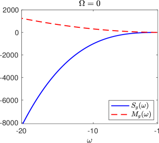
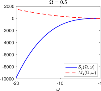
Figure 5.1. Change of the action $S_{g}(\Omega,\omega)$ and the mass $M_{g}(\Omega,\omega)$ with respect to $\omega$. Left: $\Omega=0$; Right: $\Omega=0.5$.

In the non-rotating case ($\Omega=0$), the numerical result shown in Figure 5.1 (left) illustrates the change of the action and the mass with respect to $\omega$. From the figure, one observes that the ground state mass $M_{g}(\omega)$ is strictly monotonically decreasing with respect to $\omega\in(-\infty,-\omega_{0})$ and gives a bijection from $(-\infty,-\omega_{0})$ to $(0,\infty)$. This verifies Lemmas 3.5, 3.6 and 3.7 and consequently, Theorem 3.2. In addition, the ground state action $S_{g}(\omega)$ is strictly monotonically increasing with respect to $\omega\in(-\infty,-\omega_{0})$.

In the rotating case, where we take $\Omega=0.5$, the behaviours are very similar. It is observed from Figure 5.1 (right) that, for a fixed $\Omega$, $M_{g}(\Omega,\omega)$ is still strictly monotonically decreasing with respect to $\omega$ and has the following limits:

$$M_{g}(\Omega,\omega)\to 0\quad\mbox{as }\omega\to-\lambda_{0}(\Omega)^{-},\quad M_{g}(\Omega,\omega)\to\infty\quad\mbox{as }\omega\to-\infty.$$

For a fixed $\Omega$, $S_{g}(\Omega,\omega)$ is strictly monotonically increasing with respect to $\omega$ and

$$S_{g}(\Omega,\omega)\to 0\quad\mbox{as }\omega\to-\lambda_{0}(\Omega)^{-},\quad S_{g}(\Omega,\omega)\to-\infty\quad\mbox{as }\omega\to-\infty.$$

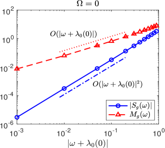
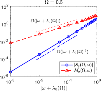
Figure 5.2. Asymptotic rates of $S_{g}(\Omega,\omega)$ and $M_{g}(\Omega,\omega)$ when $\omega\to-\lambda_{0}(\Omega)^{-}$. Left: $\Omega=0$; Right: $\Omega=0.5$.

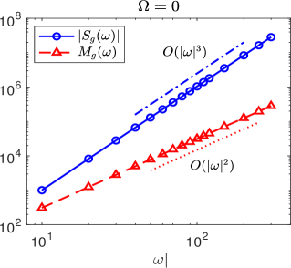
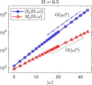
Figure 5.3. Asymptotic rates of $S_{g}(\Omega,\omega)$ and $M_{g}(\Omega,\omega)$ when $\omega\to-\infty$. Left: $\Omega=0$; Right: $\Omega=0.5$.

5.2. Asymptotics for limiting $\omega$.

Next, we investigate the asymptotic convergence rates of the ground state action and mass for limiting $\omega$.

Firstly, we consider the limit $\omega\to-\lambda_{0}(\Omega)^{-}$. As shown in Figure 5.2, the following asymptotic rates for the action and mass at the ground state are observed in both non-rotating and rotating regimes:

$$|S_{g}(\Omega,\omega)|\sim|\omega+\lambda_{0}(\Omega)|^{2},\quad M_{g}(\Omega,\omega)\sim|\omega+\lambda_{0}(\Omega)|,\quad\mbox{as }\omega\to-\lambda_{0}(\Omega)^{-}.$$

Clearly, this verifies Theorem 4.15 and Corollary 4.17 in the case of $p=3$.

Secondly, we consider the limit $\omega\to-\infty$. We can observe from Figure 5.3 (for $\Omega=0$ and $\Omega=0.5$) that,

$$|S_{g}(\Omega,\omega)|\sim|\omega|^{3},\quad M_{g}(\Omega,\omega)\sim|\omega|^{2},\quad\mbox{as }\omega\to-\infty.$$

The analysis of the two observed asymptotic rates is undergoing. As derived in Section 4.4, here we denote the Thomas-Fermi approximation of the action ground state as

$$\phi_{\omega}^{\text{TF}}(\mathbf{x})=|\omega|^{\frac{1}{2}}\tilde{\phi}\left(|\omega|^{-\frac{1}{2}}\mathbf{x}\right),\quad\tilde{\phi}(\mathbf{x})=\left[\left(1-V(\mathbf{x})\right)_{+}\right]^{\frac{1}{2}}.$$

We find that now $\|\phi_{\omega}^{\text{TF}}\|^{2}_{L^{2}}=|\omega|^{2}\|\tilde{\phi}\|^{2}_{L^{2}},$ which gives the same asymptotic rate in mass as the above numerical observation for $\omega\to-\infty$. The action value can not be predicted from $\phi_{\omega}^{\text{TF}}$ due to its non-smoothness in space. Figure 5.4 shows a one-dimensional example to illustrate the validity of the Thomas-Fermi approximation, which confirms (4.35).

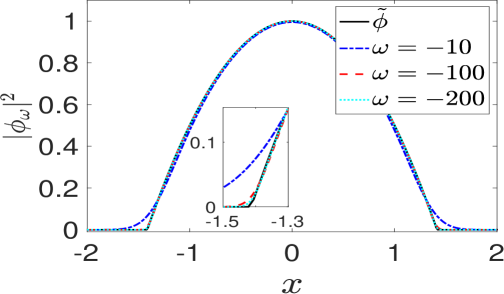
Figure 5.4. The rescaled action ground state $\tilde{\phi}_{\omega}$ (4.34) for different $\omega$ and the limit $\tilde{\phi}$.

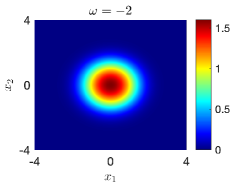
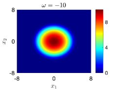
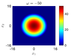
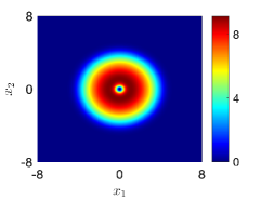
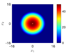
Figure 5.5. Density profiles of $|\phi_{\Omega,\omega}(x_{1},x_{2})|^{2}$ around the critical $\Omega^{c}$: $0.766<\Omega^{c}<0.767$ for $\omega=-2$ (left column), $0.292<\Omega^{c}<0.293$ for $\omega=-10$ (center column), $0.089<\Omega^{c}<0.090$ for $\omega=-50$ (right column), where the lower bounds give non-vortex states (1st row) and the upper bounds give vortex states (2nd row).

5.3. Vortices and critical angular velocity.

The rotational force in (1.1) could lead to quantized vortices in the ground state, which differs the defocusing NLS significantly from the focusing case and is of great interest in applications. The vortex phenomenon has been well studied in the context of energy ground states [4], and now we investigate the counterpart for the action ground states.

Our numerical computations show that for any $\omega<-1$, there exists a critical angular velocity $0<\Omega^{c}<1$ depending on $\omega$ such that when $0\leq\Omega<\Omega^{c}$, the density profile of action ground state is unchanged, i.e., $|\phi_{\Omega,\omega}|^{2}=\phi_{\omega}^{2}$. It remains radially symmetric, and $S_{g}(\Omega,\omega)\equiv S_{g}(\omega)=S_{g}(\Omega=0,\omega)$. This is consistent with Theorem 4.11 and is in fact a stronger result. When $\Omega>\Omega^{c}$, a radially symmetric central vortex starts to appear in the action ground state $\phi_{\Omega,\omega}$ and $S_{g}(\Omega,\omega)<S_{g}(\omega)$. These findings are demonstrated through Figure 5.5 and Figure 5.6. The former plots the density of the action ground states around the critical angular velocity $\Omega^{c}$ for $\omega=-2,-10,-50$, and the latter plots the change of the ground state action $S_{g}(\Omega,\omega)$ and mass $M_{g}(\Omega,\omega)$ with respect to $\Omega$ under $\omega=-5$. When $\Omega$ further increases, Figure 5.7 which plots the action ground states for fixed $\omega=-5$ and different $\Omega$, show that a complex vortex lattice pattern is gradually formed with the number of vortices rapidly increasing, and the density function becomes no longer radially symmetric.

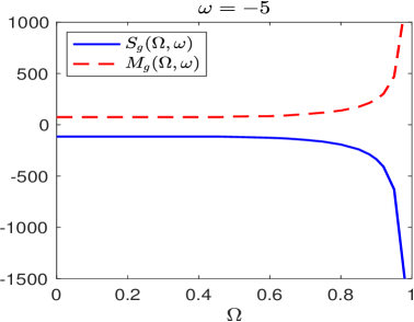
Figure 5.6. Change of $S_{g}(\Omega,\omega)$ and $M_{g}(\Omega,\omega)$ with respect to $\Omega$ under $\omega=-5$.

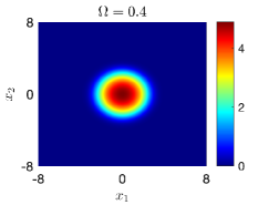
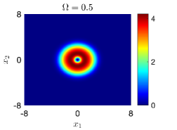
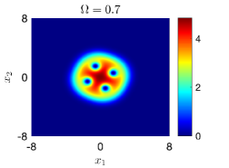
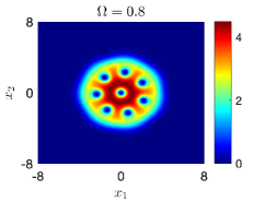
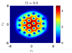
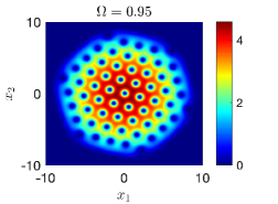
Figure 5.7. Density profiles of $|\phi_{\Omega,\omega}(x_{1},x_{2})|^{2}$ for $\omega=-5$ and different $\Omega$.

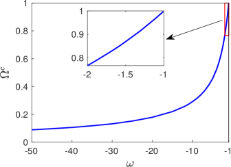
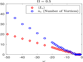
Figure 5.8. Critical angular velocity $\Omega^{c}$ as a function of $\omega$ (left); Number of vortices $n_{v}$ in $\phi_{\Omega,\omega}$ and the angular momentum expectation $\langle L_{z}\rangle$ against $\omega$ (right).

The left plot of Figure 5.8 further addresses the variation of the critical angular velocity $\Omega^{c}$ with respect to $\omega$. It can be observed that $\Omega^{c}$ increases monotonically as $\omega$ increases, and

$$\lim_{\omega\to-\infty}\Omega^{c}=0,\qquad\lim_{\omega\to-1^{-}}\Omega^{c}=1.$$

Thus, for $\omega$ in the limit regime $\omega\to-\infty$, a very small $\Omega>0$ can trigger vortices in the action ground states. To understand the change of vortices in the action ground state with respect to $\omega$, we fix $\Omega=0.5$ and plot in the right part of Figure 5.8 the number of vortices $n_{v}$ and the angular momentum expectation, i.e., $\langle L_{z}\rangle:=\frac{1}{\|\phi_{\Omega,\omega}\|_{L^{2}}^{2}}\int_{\mathbb{R}^{2}}\overline{\phi_{\Omega,\omega}}L_{z}\phi_{\Omega,\omega}\,\mathrm{d}\mathbf{x}$, against several $\omega$. We can see that both $n_{v}$ and $\langle L_{z}\rangle$ show an approximately linear increase as $\omega\to-\infty$.

Table 5.1. Quantitative results obtained from the action ground state for three different $\omega$ and the corresponding energy ground state.

$\omega$	$S_{g}$	$m$	$E_{g}$	$\mu_{g}$	$e^{\text{rel}}_{\omega}$	$e^{\text{rel}}_{S}$
$-30$	$-34342.56$	$3517.33$	$71177.33$	$30.00$	$3.21\times 10^{-10}$	$7.31\times 10^{-14}$
$-40$	$-82943.09$	$6335.55$	$170478.80$	$40.00$	$6.59\times 10^{-10}$	$4.82\times 10^{-14}$
$-50$	$-163950.62$	$9997.17$	$335907.93$	$50.00$	$2.21\times 10^{-10}$	$2.38\times 10^{-14}$

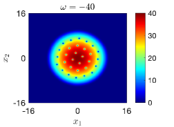
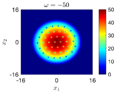
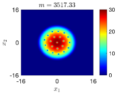
Figure 5.9. Density profiles of the action ground state $|\phi_{\Omega,\omega}(x_{1},x_{2})|^{2}$ (top row) and the corresponding energy ground state $|\phi_{m}^{E}(x_{1},x_{2})|^{2}$ (bottom row).

5.4. Relation with energy ground state and evidence of non-equivalence

Finally, we examine the relation between the action and the energy ground states. Here we fix $\Omega=0.5$.

1) Conditional equivalence. For a given $\omega$, we begin by computing the action ground state $\phi_{\Omega,\omega}$ and obtain its action $S_{g}=S_{g}(\Omega,\omega)$ and mass $m=M_{g}(\Omega,\omega)$. We then compute the energy ground state $\phi_{m}^{E}$ with the mass $m$ and obtain the corresponding ground state energy $E_{g}=E(\phi_{m}^{E})$ and chemical potential $\mu_{g}=\mu(\phi_{m}^{E})$ (1). We now compare the obtained results from the action and the energy ground states. The relative differences $e^{\text{rel}}_{\omega}=|\omega-(-\mu_{g})|/|\omega|$ and $e^{\text{rel}}_{S}=|S_{g}-(E_{g}+m\omega)|/|S_{g}|$ for $\omega=-30,-40,-50$ are listed in Table 5.1. The density profiles of $\phi_{\Omega,\omega}$ and $\phi_{m}^{E}$ are shown in Figure 5.9. From Figure 5.9 and Table 5.1, one can observe that, for these values of $\omega$, the wave function and related physical quantities all form a precise loop from the action ground state to the energy ground state and then to the action ground state, since $\omega\approx-\mu_{g}$ and $S_{g}\approx E_{g}+m(-\mu_{g})$ within numerical precision. This matches Theorem 4.1.

2) Evidence of non-equivalence. We provide an evidence for the non-equivalence described in Theorem 4.9 by investigating the mass of the action ground state on a finer mesh for $\omega$. As shown in Figure 5.10 for fixed $\Omega=0.5$, there are a series of critical values of $\omega$, i.e., $\omega_{\mathrm{cr}}^{1}=-4.3490$, $\omega_{\mathrm{cr}}^{2}=-6.9025$, $\omega_{\mathrm{cr}}^{3}=-7.8835$, etc., such that the mass of the action ground state $\|\phi_{\Omega,\omega}\|_{L^{2}}^{2}$ has jump discontinuities near these critical values, indicating the existence of multiple action ground states with different mass values at them. More precisely, it is observed that the mass behaves near these critical values as follows:

$$\|\phi_{\Omega,\omega}\|_{L^{2}}^{2}<55.4535,\quad\mbox{if }\omega>\omega_{\mathrm{cr}}^{1},\quad\|\phi_{\Omega,\omega}\|_{L^{2}}^{2}>59.6198,\quad\mbox{if }\omega<\omega_{\mathrm{cr}}^{1};$$

$$\|\phi_{\Omega,\omega}\|_{L^{2}}^{2}<156.3416,\;\;\mbox{if }\omega>\omega_{\mathrm{cr}}^{2},\quad\|\phi_{\Omega,\omega}\|_{L^{2}}^{2}>161.2327,\;\;\mbox{if }\omega<\omega_{\mathrm{cr}}^{2};$$

$$\|\phi_{\Omega,\omega}\|_{L^{2}}^{2}<211.8255,\;\;\mbox{if }\omega>\omega_{\mathrm{cr}}^{3},\quad\|\phi_{\Omega,\omega}\|_{L^{2}}^{2}>216.2082,\;\;\mbox{if }\omega<\omega_{\mathrm{cr}}^{3};\quad\cdots,$$

and there is no action ground state with a mass value coming from the range

$$\big{(}55.4535,59.6198\big{)}\bigcup\big{(}156.3416,161.2327\big{)}\bigcup\big{(}211.8255,216.2082\big{)}\bigcup\cdots.$$ (5.1)

It is worthwhile to point out that these critical values $\omega_{\mathrm{cr}}^{j}$ are exactly the transition points where the number of vortices in the action ground state increases. See the density profiles shown in Figure 5.10. The first critical value $\omega_{\mathrm{cr}}^{1}$ corresponds exactly to the critical rotational speed $\Omega^{c}$ discussed in Section 5.3.

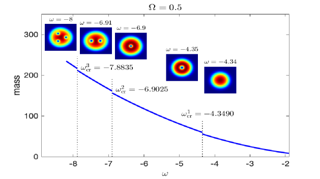
Figure 5.10. Change of the mass $\|\phi_{\Omega,\omega}\|_{L^{2}}^{2}$ with respect to $\omega$ and density profiles $|\phi_{\Omega,\omega}(x_{1},x_{2})|^{2}$ at $\omega=-4.34,-4.35,-6.9,-6.91,-8$ when $\Omega=0.5$.

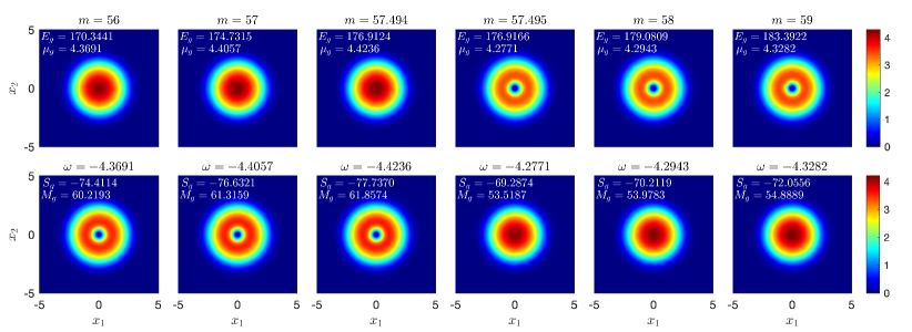
Figure 5.11. Density profiles of the energy ground state $|\phi_{m}^{E}(x_{1},x_{2})|^{2}$ (1st row) and the corresponding action ground state $|\phi_{\Omega,\omega}(x_{1},x_{2})|^{2}$ (2nd row) with $\omega=-\mu_{g}$.

As predicted by Theorem 4.9, any energy ground state $\phi_{m}^{E}$ within the given mass range (5.1) must not be an action ground state. To verify this, Figure 5.11 presents the numerical results for energy ground states $\phi_{m}^{E}$ with several $m\in(55.4535,59.6198)$ and the corresponding action ground states $\phi_{\Omega,\omega}$ with $\omega=-\mu(\phi_{m}^{E})$. The results show that for these values of $m$ (corresponding to $\omega=\omega_{\mathrm{cr}}^{1}$), the wave function and related physical quantities cannot loop from the energy ground state to the action ground state and then back to the original energy ground state. In addition, we observe that there exists a critical value of mass $m_{\mathrm{cr}}^{1}\in(57.494,57.495)$ such that, for given $m\in(55.4535,59.6198)$, the chemical potential $\omega=-\mu(\phi_{m}^{E})$ and the mass of corresponding action ground state satisfy:

1. when $m\in(55.4535,m_{\mathrm{cr}}^{1})$, $\omega=-\mu(\phi_{m}^{E})<\omega_{\mathrm{cr}}^{1}$ and $\|\phi_{\Omega,\omega}\|_{L^{2}}^{2}>59.6198$;

2. when $m\in(m_{\mathrm{cr}}^{1},59.6198)$, $\omega=-\mu(\phi_{m}^{E})>\omega_{\mathrm{cr}}^{1}$ and $\|\phi_{\Omega,\omega}\|_{L^{2}}^{2}<55.4535$.

In Figure 5.11, the energy ground states displayed in the top row, while bearing a resemblance to the action ground states depicted in the bottom row, are in fact not action ground states. Nevertheless, these energy ground states are still nontrivial solutions to the stationary RNLS (1.3) with $\omega=-\mu(\phi_{m}^{E})$, and their action values are higher than the ground states, which indicates that they are action excited states. For example, for $m=57.494$, from Figure 5.11, $S_{\Omega,\omega}(\phi_{m}^{E})=E_{g}-m\mu_{g}=176.9124-57.494\times 4.4236=-77.4181>S_{g}=-77.7370$.

6. Conclusion

We studied the action ground states of the rotating nonlinear Schrödinger equation in defocusing nonlinear interaction case. Theoretical analysis has been done to understand the relation between the action ground states and the energy ground states. In the absence of rotating force, i.e, the non-rotating case, the complete equivalence of the two kinds of ground states has been established. For the rotating case, a conditional equivalence has been proved and a characterization for possible occurrence of non-equivalence has been derived. Along with the analysis, the asymptotic behaviours of the mass and the action at the ground state solution have also been obtained in some limit regimes. Numerical experiments have been conducted to verify the theoretical studies and investigate the vortices phenomena in action ground states. Moreover, we have numerically observed strong evidence of non-equivalence between the action ground state and the energy ground state.

Appendix A A fact of ground-state energy under symmetric harmonic oscillator

Lemma A.1.

If $V(\mathbf{x})=\frac{1}{2}\gamma_{r}^{2}|\mathbf{x}|^{2}$ ($d=2$), and $|\Omega|<\gamma_{r}$, then $\lambda_{0}(\Omega)\equiv\lambda_{0}(0)=\gamma_{r}$ with the corresponding eigenfunction $\varphi_{0}=\sqrt{\gamma_{r}/\pi}\mathrm{e}^{-\gamma_{r}|\mathbf{x}|^{2}/2}$ up to a constant phase factor. If $V(\mathbf{x})=\frac{1}{2}\gamma_{r}^{2}(x_{1}^{2}+x_{2}^{2})+\frac{1}{2}\gamma_{3}x_{3}^{2}$ ($d=3$), $\gamma_{3}>0$, and $|\Omega|<\gamma_{r}$, then $\lambda_{0}(\Omega)\equiv\lambda_{0}(0)=\gamma_{r}+\frac{1}{2}\gamma_{3}$ with the corresponding eigenfunction $\varphi_{0}=\frac{\gamma_{r}^{1/2}\gamma_{3}^{1/4}}{\pi^{3/4}}\mathrm{e}^{-\gamma_{r}(x_{1}^{2}+x_{2}^{2})/2-\gamma_{3}x_{3}^{2}/2}$ up to a constant phase factor.

Proof.

Direct computations show that, in 2D polar coordinate $(r,\theta)$, all the eigenvalues and corresponding eigenfunctions of $R=-\frac{1}{2}\Delta+\frac{1}{2}\gamma_{r}^{2}|\mathbf{x}|^{2}-\Omega L_{z}$ are given as [6]

$$\lambda_{mn}(\Omega)=(2n+|m|+1)\gamma_{r}-m\Omega,\quad\varphi_{mn}(r,\theta)=C_{mn}r^{|m|}\mathcal{L}_{n}^{(|m|)}(\gamma_{r}r^{2})\mathrm{e}^{-\gamma_{r}r^{2}/2}\mathrm{e}^{im\theta},\quad n\in\mathbb{N},\,m\in\mathbb{Z},$$

where $\mathcal{L}_{n}^{(|m|)}$ are generalized Laguerre polynomials and $C_{mn}>0$ are normalization constants such that $\|\varphi_{mn}\|_{L^{2}}=1$. Since $|\Omega|<\gamma_{r}$, the smallest eigenvalue is $\lambda_{0}(\Omega)=\lambda_{00}(\Omega)=\gamma_{r}$, which is single-fold, with the corresponding eigenfunction $\varphi_{00}(r,\theta)=\sqrt{\gamma_{r}/\pi}\mathrm{e}^{-\gamma_{r}r^{2}/2}$. The proof in 3D can be done by using the cylindrical coordinate $(r,\theta,x_{3})$ and noting that $-\frac{1}{2}\partial_{x_{3}}^{2}+\frac{1}{2}\gamma_{3}^{2}x_{3}^{2}$ has eigenvalues $\left(k+\frac{1}{2}\right)\gamma_{3}$ ($k\in\mathbb{N}$) with corresponding eigenfunctions given by scaled Hermite functions [6]. ∎

Note that $\lambda_{0}(\Omega)$ can be viewed as the ground-state energy of a non-interacting rotating BEC [4]. Lemma A.1 says that under a 2D radially symmetric or 3D cylindrical symmetric harmonic oscillator potential, the ground state is independent of the rotational speed $\Omega$.

References

- [1] A.H. Ardila, H. Hajaiej, Global well-posedness, blow-up and stability of standing waves for supercritical NLS with rotation, J. Dynam. Differential Equations 35 (2023) pp. 1643-1665.
- [2] P. Antonelli, D. Marahrens, C. Sparber, On the Cauchy problem for nonlinear Schrödinger equation with rotation, Discrete Contin. Dyn, Syst. 32 (2012) pp. 703–715.
- [3] J. Arbunich, I. Nenciu, C. Sparber, Stability and instability properties of rotating Bose-Einstein condensates, Lett. Math. Phys. 109 (2019) pp. 1415-1432.
- [4] W. Bao, Y. Cai, Mathematical theory and numerical methods for Bose-Einstein condensation, Kinet. Relat. Models 6 (2013) pp. 1-135.
- [5] W. Bao, Q. Du, Y. Zhang, Dynamics of rotating Bose-Einstein condensates and their efficient and accurate numerical computation, SIAM J. Appl. Math. 66 (2006) pp. 758-786.
- [6] W. Bao, H. Li, J. Shen, A generalized Laguerre-Fourier-Hermite pseudospectral method for computing the dynamics of rotating Bose-Einstein condensates, SIAM J. Sci. Comput. 31 (2009) pp. 3685-3711.
- [7] W. Bao, H. Wang, P.A. Markowich, Ground, symmetric and central vortex states in rotating Bose-Einstein condensates, Comm. Math. Sci. 3 (2005) pp. 57-88.
- [8] H. Berestycki, P.L. Lions, Nonlinear scalar field equations I: Existence of a ground state, Arch. Rat. Mech. Anal. 82 (1983) pp. 313-345.
- [9] H. Berestycki, P.L. Lions, Nonlinear scalar field equations II: Existence of infinitely many solutions, Arch. Rat. Mech. Anal. 82 (1983) pp. 347-375.
- [10] H. Chen, G. Dong, W. Liu, Z. Xie, Second-order flows for computing the ground states of rotating Bose-Einstein condensates, J. Comput. Phys. 475 (2023) 111872.
- [11] S. Dovetta, E. Serra, P. Tilli, Action versus energy ground states in nonlinear Schrödinger equations, Math. Ann. 385 (2023) pp. 1545–1576.
- [12] A.L. Fetter, Rotating trapped Bose-Einstein condensates, Rev. Mod. Phys. 81 (2009) pp. 647-691.
- [13] R. Fukuizumi, Stability and instability of standing waves for the nonlinear Schrödinger equation with harmonic potential, Discrete Contin. Dyn. Syst. 7 (2001) pp. 525-544.
- [14] R. Fukuizumi, M. Ohta, Stability of standing waves for nonlinear Schrödinger equations with potentials, Differ. Integral Equ. 16 (2003) pp. 111-128.
- [15] R. Fukuizumi, M. Ohta, Instability of standing waves for nonlinear Schrödinger equations with potentials, Differ. Integral Equ. 16 (2003) pp. 691-706.
- [16] E.H. Lieb, M. Loss, Analysis, 2nd ed., Graduate studies in Mathematics, Amer. Math. Soc. 2001.
- [17] E.H. Lieb, R. Seiringer, J. Yngvason, Bosons in a trap: A rigorous derivation of the Gross-Pitaevskii energy functional, Phys. Rev. A 61 (2000) 043602.
- [18] W. Liu, Y. Cai, Normalized gradient flow with Lagrange multiplier for computing ground states of Bose-Einstein condensates, SIAM J. Sci. Comput. 43 (2021) pp. B219-B242.
- [19] W. Liu, Y. Yuan, X. Zhao, Computing the action ground state for the rotating nonlinear Schrödinger equation, SIAM J. Sci. Comput. 45 (2023) pp. A397-A426.
- [20] L. Jeanjean, S. Lu, On global minimizers for a mass constrained problem, Calc. Var. Partial Differential Equations 64 (2022) 214.
- [21] H. Matsumoto, N. Ueki, Spectral analysis of Schrödinger operators with magnetic fields, J. Funct. Anal. 140 (1996) pp. 218-255.
- [22] A. Mohamed, G. Raikov, On the spectral theory of the Schrödinger operator with electromagnetic potential, in pseudo-differential calculus and mathematical physics, vol. 5 of Math. Top., Akademie Verlag, Berlin (1994) pp. 298–390.
- [23] J. Shatah, W. Strauss, Instability of nonlinear bound states, Comm. Math. Phys. 100 (1985) pp. 173-190.
- [24] W.A. Strauss, Existence of solitary waves in higher dimensions, Comm. Math. Phys. 55 (1977), pp. 149-162.
- [25] R. Seiringer, Gross-Pitaevskii theory of the rotating Bose gas, Comm. Math. Phys. 229 (2002) pp. 491-509.
- [26] C. Wang, Computing the least action ground state of the nonlinear Schrödinger equation by a normalized gradient flow, J. Comput. Phys. 471 (2022) 111675.