Fluctuation in the Fidelity of Information Recovery from Hawking Radiation
Abstract
The interior of a pure-state black hole is known to be reconstructed from the Petz map by collecting a sufficiently large amount of the emitted Hawking radiation. This was established based on the Euclidean replica wormhole, which comes from an ensemble averaging over gravitational theories. On the other hand, this means that the Page curve and the interior reconstruction are both ensemble averages; thus, there is a possibility of large errors. In the previous study Bousso:2023efc , it was shown that the entropy of the Hawking radiation has fluctuation of order , thus is typical in the ensemble. In the present article, we show that the fluctuations of the relative entropy difference in the encoding map and the entanglement fidelity of the Petz map are both suppressed by compared to the signals, establishing the typicality in the ensemble. In addition, we also compute the entanglement loss of the encoding map.
1 Introduction
In AdS/CFT, the entanglement entropy of a boundary subregion is given by the area of the Ryu-Takayanagi surface , called Ryu-Takayanagi formula Ryu:2006bv ; Hubeny:2007xt ; Faulkner:2013ana ; Engelhardt:2014gca . The bulk subregion bounded by and , is called the entanglement wedge of , and it corresponds to the boundary subregion in the following sense: the information on can be embedded in the boundary subregion , and there is an approximate inverse which reconstructs the original bulk information. This whole process is called entanglement wedge reconstruction Czech:2012bh ; Almheiri:2014lwa ; Pastawski:2015qua ; Jafferis:2015del ; Dong:2016eik ; Hayden:2016cfa ; Harlow:2016vwg ; Cotler:2017erl ; Chen:2019gbt .
This existence of an approximate recovery map is crucial in the recovery of the bulk information from the boundary state. It is guaranteed due to the fact that the relative entropy difference between the bulk and the boundary states is sufficiently small Jafferis:2015del , which means the bulk information is faithfully encoded in the boundary. When there is an approximate recovery map, then the Petz map is known to be an approximate inverse map whose error is in the same order Barnum , and thus, we can use the Petz map to reconstruct interior information from the boundary. This means, in general situations, it is sufficient to study the fidelity of the Petz map when we need to check if there is an approximate recovery map or not.
It was noticed later that the entanglement wedge reconstruction can be applied to retrieving the interior information of the black hole Penington:2019npb ; Almheiri:2019psf ; Almheiri:IslandFormula ; Penington:ReplicaWormholeWestCoast ; Almheiri:ReplicaWormholeEastCoast , see also Vardhan:2021mdy ; Balasubramanian:2022fiy ; Akers:2022qdl ; Czech:2023rbh ; Nakayama:2023kgr for recent treatments. It was found that the information inside the black hole horizon sufficiently after the Page time is encoded in the Hawking radiation and, thus, can be recovered using the entanglement wedge reconstruction from the Hawking radiation. The earlier special version of this reconstruction is the Hayden-Preskill protocol Hayden:2007cs , where the size of the interior information remains Hayden:2018khn . In the present case, it was found in Penington:ReplicaWormholeWestCoast that the interior information, whose dimension scales as the dimension of the black hole, can be recovered via the Petz map in accord with Hayden:2018khn .
In the derivations of the Page curve and of the reconstruction of the interior information, the Euclidean replica wormholes played a crucial role. These Euclidean wormholes were found to bring a new important puzzle since the gravitational path-integral over Euclidean wormholes cannot be dual to quantum mechanics, but instead dual to an ensemble of boundary quantum theories Maldacena:2004rf ; Maldacena:2004rf ; Saad:2018bqo ; Saad:2019pqd ; Harlow:2018tqv ; Bousso:2019ykv ; Bousso:2020kmy . This implies that the gravity theory with Euclidean wormholes is also an ensemble of quantum gravity theories. In the ensemble of theories, the physical quantities are all ensemble averages. Thus, the computed Page curve and the fidelity of the Petz map are both averages in the ensemble, and there is no guarantee that they are typical answers in the ensemble. In other words, it is possible that these quantities are significantly different from the averaged answers for typical theories in the ensemble. A famous example of such a large deviation can be seen in the ramp and the plateau of the spectral form factor, where the error and the average answer are in the same order. Therefore, the fundamental question to ask in the black hole information problem is whether the ensemble averages of these quantities are typical or not in the ensemble.
In Bousso:2023efc , this question on the typicality of the Page curve was addressed. It was shown that the average noise in the entropy of the Hawking radiation is always of order , where is the black hole entropy. This means that the fluctuation is proportional to the inverse of the Hilbert space dimension. Therefore, the ensemble average of the Page curve is highly typical in the ensemble.
In this paper, we ask another important question in the typicality, namely that of interior information recovery. We will show that the reconstruction of the interior information after the Page time is possible in the typical member of the ensemble. We show this by studying the fluctuations of the measures of the information recovery, namely the relative entropy difference and the entanglement fidelity of the Petz recovery map. When the relative entropy difference is sufficiently small or the entanglement fidelity is close to one, we can tell that the information recovery from the interior is possible. These measures are known to take those values in average sufficiently after the Page time, but so far the typicality of that behavior has not been discussed. We found that such behavior is indeed typical in the ensemble, namely, if we take a member in the ensemble, then the information recovery is typically possible. We show this by studying the fluctuations of these measures and find that they are suppressed by the factor compared to the signals. This implies that the success of the information recovery is also highly typical in the ensemble.
The organization of this paper is as follows. In section 2, we explain fundamental notions and measures of the interior information recovery, such as the relative entropy difference, the entanglement fidelity, the Petz map, and the coherent quantum information. We will explain why these are so important in the reconstruction by explaining the fundamental inequalities they satisfy. In section 3, we review the PSSY model, which is the model of a black hole entangled with its Hawking radiation. We will also review the fluctuation of the Page curve in the PSSY model studied in Bousso:2023efc . In section 4, we present our main result of this paper, namely, we evaluate the fluctuations of the relative entropy difference and the entanglement fidelity of the Petz map.
2 Measures of the Interior Information Recovery
In this section, we will review some important notions and measures in interior information recovery. We will briefly explain the quantum error correction and the Petz map, which are nothing but the entanglement wedge reconstruction and the bulk recovery map when applied to gravity. We then explain how it can be studied using the relative entropy difference, the entanglement fidelity, and the coherent quantum information. Readers who are familiar with their properties can skip this section.
2.1 Quantum Error Correction and the Petz Map
In quantum error correction, we consider embedding quantum information into a larger system to protect the information against possible errors. In the entanglement wedge reconstruction of the black hole interior, the quantum information of the interior excitations is embedded into the Hawking radiation. The bulk interior quantum information lives in a Hilbert space as a density matrix on . This Hilbert space is called code subspace, and the space of quantum states on is denoted as . Now, the quantum information on is embedded into the larger one . corresponds to the Hilbert space of the Hawking radiation. The embedding map is called the encoding map. The encoding map is a completely positive trace preserving (CPTP) map, meaning that any entangled quantum state should be mapped to an entangled quantum state. We will call a CPTP map as a channel as well.
In order to recover the interior information from the Hawking radiation, we need to find a CPTP map that satisfies
| (2.1) |
so that the embedded information can be reconstructed using . Such map is called an approximate recovery map for . As we will explain shortly, it is known that the Petz map can be used as a good approximate recovery map whenever there is an approximate recovery map. Thus, we can use the Petz map as an explicit realization of the approximate recovery map. To write down the Petz map, we need to fix a , and the Petz map depends on . The Petz map is explicitly given by
| (2.2) |
Here is the adjoint defined by . It is clear that the Petz map recovers the reference state, namely holds.
2.2 Entanglement Fidelity and the Petz Map
The fidelity of the channel is widely used in quantum information theory in order to measure the difference between channels. In particular, we will be interested in the difference between and , in order to measure how well can recover the original information encoded by . For this purpose, we consider the entanglement fidelity of a channel of a state , defined by
| (2.3) |
here we used arbitrary purification of . Note that this definition does not depend on the choice of the purification. The entanglement fidelity depends on the state and does not capture the worst case deviation from the identity channel, in contrast to the minimum fidelity 111The minimum fidelity measures the worst case deviation of the channel from the identity channel , and is defined by (2.4) By definition, it is clear that (2.5) and iff . The entanglement fidelity gives a lower bound on the minimum fidelity when the Hilbert space is appropriately restricted. More explicitly, it can be shown that for each there exist a -dimensional subspace and associated projection , such that for the restricted channel (2.6) the inequality (2.7) holds Kretschmann_2004 ; 5429118 . Here we used the standard p-norm . If we take the maximally mixed state and in this theorem, we obtain (2.8) Thus, once we show the entanglement fidelity is sufficiently close to , then we can automatically see the fidelity on a restricted subspace is also close to . The important point here is that there is no dimension-dependent factor in this inequality, which would prohibit us from considering large code subspace dimension, for instance.. By definition, it is clear that.
| (2.9) |
and iff . Thus, we can see that the entanglement fidelity measures the closeness of to the identity on the support of .
Now, we use the entanglement fidelity to measure how well the Petz map recovers the original information, compared to arbitrary channel . Indeed, if the map is an approximate recovery map, then the Petz map is known to be an equally good approximate recovery map shown in Barnum . Namely, there is an inequality
| (2.10) |
This implies, if , then . Thus, the Petz map is always as good as the best approximate recovery map in terms of entanglement fidelity. In the black hole interior reconstruction, we will use the entanglement fidelity to see if the Petz map can indeed recover the interior information.
2.3 Reversibility and the Relative Entropy Difference
Without using the explicit Petz map, we can tell whether there is an approximate recovery map or not by considering reversibility measures. One such measure is the relative entropy difference. Consider quantum states and the encoding map . The relative entropy is defined by
| (2.11) |
which measures the difference between the two states. The relative entropy difference is
| (2.12) |
which is guaranteed to be non-negative due to the monotonicity of the relative entropy. When the encoding map is erroneous, then the difference between states and will be lost, resulting in an increase of the relative entropy difference.
Conversely, if the relative entropy difference is small enough, then it is known that the averaged rotated Petz map, which only depends on the reference state , is an approximate recovery map for . Indeed, it is known that the averaged rotated Petz map satisfies, for all satisfying Junge:2015lmb
| (2.13) |
Here the fidelity is defined by
| (2.14) |
where are arbitrary purifications of . It is clear that , and iff . The fidelity measures the difference between quantum states. Thus (2.13) implies that when the relative entropy is small, the fidelity is close to one, ensuring the information recovery.
| (2.15) |
In the black hole interior reconstruction, we will use the relative entropy difference to see if a map that reconstructs the interior information exists.
2.4 Reversibility and the Entanglement Loss
Next, we describe another reversibility measure called coherent information loss. When the coherent information loss is small, it is guaranteed that there is an approximate recovery map. The result in this subsection will be used in subsection 4.4.
We first describe the coherent information loss. For quantum state and the encoding map , the coherent information is defined by
| (2.16) |
here we consider an arbitrary purification of . Then coherent information loss is defined by
| (2.17) |
The coherent information loss measures the information loss in the encoding map. Indeed, if the coherent information loss is small, then there is a map which recovers the original information. Indeed, the entanglement fidelity is lower bounded as schumacher2002
| (2.18) |
Thus, if the coherent information loss is sufficiently small, then there exists a map such that . In other words, is an approximate recovery map in terms of the entanglement fidelity when the coherent information loss is sufficiently small 222This existence criterion for the recovery channel is equivalent to the decoupling criterion. To see this, let us use the Stinespring dilatation and express the channel as a unitary map on an extended Hilbert space as (2.19) We then consider the purification . Then we obtain the pure state . Using the quantum state on , the coherent information loss is rewritten as (2.20) Thus vanishing coherent information loss is equivalent to the factorization (2.21) Thus, the factorization (2.21) is equivalent to the existence of the exact recovery map, and this condition (2.21) for the information recovery is called the decoupling criterion..
The coherent information can be replaced by other correlation measures, such as mutual information, or entanglement measures like squashed entanglement. For the mutual information loss , similar to the coherent information loss, we have PhysRevA.77.012309 ; FB
| (2.22) |
Thus, when the mutual information loss is small, there exists an approximate recovery map .
3 The PSSY Model
In the present section, we review the PSSY model Penington:ReplicaWormholeWestCoast , which is a toy model of the black hole entangled with Hawking radiation. The model consists of the JT gravity Teitelboim:1983ux ; Jackiw:1984je ; Maldacena:2016upp ; Stanford:2017thb ; Yang:2018gdb ; Saad:2019lba ; Stanford:2019vob ; Saad:2019pqd with an end-of-the-world (EOW) brane in bulk anchored at the boundary. The EOW brane has flavors and tension . The action is
| (3.1) |
where
| (3.2) |
| (3.3) |
with the standard asymptotic boundary condition
| (3.4) |
with being the boundary Euclidean time. When analytically continued to Lorentzian time, the EOW brane plays the role of a particle with a flavor behind the black hole horizon. In terms of boundary quantum mechanics, is a random sum over energy eigenstates of a Hamiltonian in the matrix integral dual to the JT gravity Penington:ReplicaWormholeWestCoast
| (3.5) |
Here is a complex Gaussian random matrix of entries, and is a continuous function of , which defines the ensemble of states such as a microcanonical ensemble. EOW brane states with different flavors are nearly orthogonal but have a small overlap of order . This small overlap accounts for the finiteness of the gravity Hilbert space dimension . The accumulation of these small overlaps results in the unitary Page curve of the Hawking radiation.
In the PSSY model, one considers a state in which the EOW brane flavor is maximally entangled with an auxiliary non-gravitating system
| (3.6) |
Note that the state (3.6) is always normalized. The reduced density matrix of the radiation is
| (3.7) |
3.1 JT Gravity Partition Functions
For reference, we briefly review the JT gravity partition functions in a microcanonical ensemble with EOW branes. For full details, we refer to Bousso:2023efc . We first introduce a continuous smearing function to define a microcanonical ensemble. The smearing function is defined as
| (3.8) |
This smearing is introduced in order to suppress contributions from higher genus contributions in the fluctuations. We note that this smearing is unnecessary for the evaluations of Renyi entropy, relative entropy, and Petz fidelity.
We first consider the disk partition function. The normalized density of states of the disk is
| (3.9) |
Replacing the geodesic boundaries by EOW branes with action , we obtain the bulk partition function
where we define
| (3.11) |
for . Thus, the microcanonical partition function with boundaries is given by
| (3.12) |
Here we denote
| (3.13) |
which is the number of states in the microcanonical window. Next, we consider geometries with a single double trumpet. Defining
| (3.14) |
the partition function of a single tubular wormhole exchange between two disk topology - and -boundary partition functions is given by
| (3.15) | |||||
By considering microcanonical ensemble with the smearing function, we arrive at
In the following, we will always consider microcanonical ensemble with smearing function and take large and limit.
3.2 Entropy and its Fluctuation
Utilizing the partition function of the JT gravity with EOW branes in the last subsection, the Renyi entropy of the Hawking radiation was evaluated. Then, it is possible to evaluate the entropy of the Hawking radiation Penington:ReplicaWormholeWestCoast and its fluctuation Bousso:2023efc . From the results, we can conclude that the entropy and the rank of the Hawking radiation are typical in the ensemble.
The entropy of the Hawking radiation is
| (3.17) |
and the rank of the Hawking radiation state is given by
| (3.18) |
The fluctuation of the entropy is given by
| (3.19) |
Thus, the entropy fluctuation is always of order . This behavior is distinct from the random pure state, whose entropy fluctuation decays as at large . We can understand this behavior by noticing the fluctuation of the number of states in the given microcanonical window, which is given by the rank fluctuation at large . The fluctuation of the rank is
| (3.20) |
which is non-zero only after the Page time . Thus, the square of the fluctuation of the number of states depends logarithmically on the ratio .
4 Fluctuations in the Measures of the Interior Information Recovery
In this section, we consider the reconstruction of the interior information using the Petz map. It was found that by applying the Petz map to the Hawking radiation after the Page time, the interior information can be reconstructedPenington:ReplicaWormholeWestCoast , see also Hayden:2007cs ; Hayden:2018khn . The recovery of the interior information can be confirmed by the relative entropy difference, the entanglement fidelity of the Petz map, and the coherent information loss.
The primary goal of this paper is to study the fluctuations of these measures of interior information recovery, in particular, the relative entropy difference and the entanglement fidelity of the Petz map. By studying these fluctuations, we reveal that interior reconstruction is indeed possible among the typical members of the ensemble. We also present a computation of the coherent information loss and the mutual information loss, which guarantee that the information recovery is possible on average.
This section consists of four subsections. We first review how the interior information is encoded in the Hawking radiation state. Then, we study the fluctuations of the relative entropy difference and the entanglement fidelity of the Petz map. Finally, we attach a computation of the measures of the entanglement loss.
4.1 Encoding Information in the PSSY Model
We now review how to encode interior quantum information into the Hawking radiation in the PSSY model. For this purpose we generalize the total pure state (3.6) to have indices from the code subspace
| (4.1) |
Here the EOW brane states have indices . The boundary description of this state can be obtained by replacing by in (3.5). These new indices now carry interior information. A quantum state on the code subspace is now encoded in the Hawking radiation via the encoding map defined by
| (4.2) |
In particular, the action of the encoding map on the maximally mixed reference state is
| (4.3) |
Here we defined .
The question of the information recovery is whether there is an approximate inverse of , recovering the original state from . This is indeed the case when corresponds to the late time after the Page time. In the following, we assume that late time, namely .
4.2 Relative Entropy Difference
We first study the relative entropy difference for . Small relative entropy difference guarantees that the averaged rotated Petz map is an approximate recovery map for . We first review that the relative entropy difference is indeed small at .
For simplicity, we consider encoding a pure state in the Hawking radiation. We fix the reference state as , and consider the relative entropy difference
| (4.4) |
where . Since we have , we only need to evaluate . This can be accomplished by employing the replica trick
| (4.5) |
We can explicitly write
| (4.6) | |||||
The evaluation of this quantity can be done in the same way as the computation of the Page curve, replacing by . Thus, by combining terms, the relative entropy difference is Vardhan:2021mdy
| (4.7) |
In particular, at , the error in the encoding map is small, and the Petz map is an approximate recovery map.
The main purpose of this paper is to understand whether this relative entropy difference is typically small in the ensemble. It suffices to study the fluctuation of the relative entropy . The fluctuation is given by
Here, we denote the ensemble average by . We compute this quantity by evaluating wormhole configurations at . The first contribution
| (4.9) |
is identical to the fluctuation of the entropy (3.19). The second contribution
| (4.10) |
is again identical to the fluctuation of the entropy (3.19) with being replaced by . The third contribution
| (4.11) |
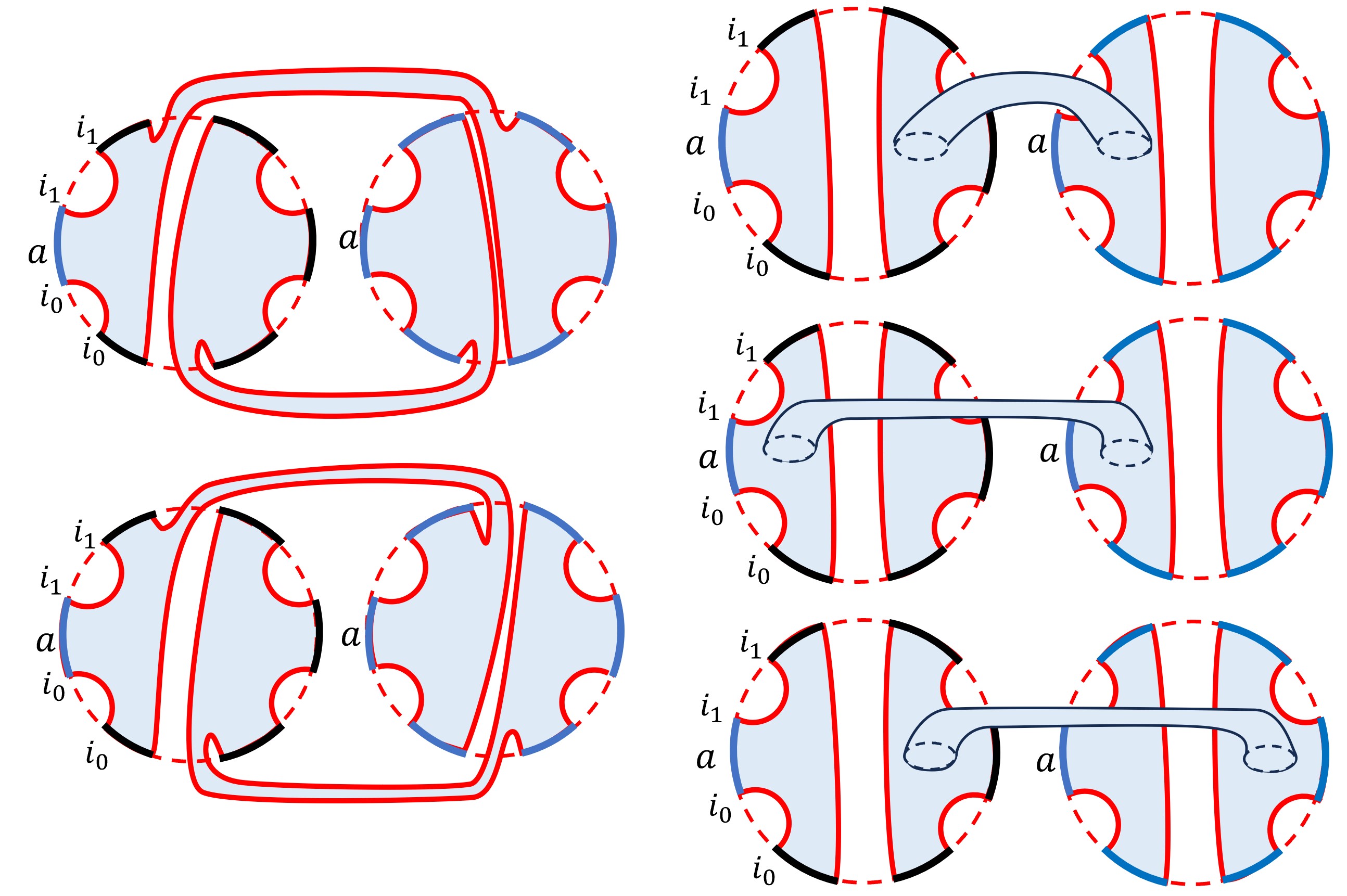
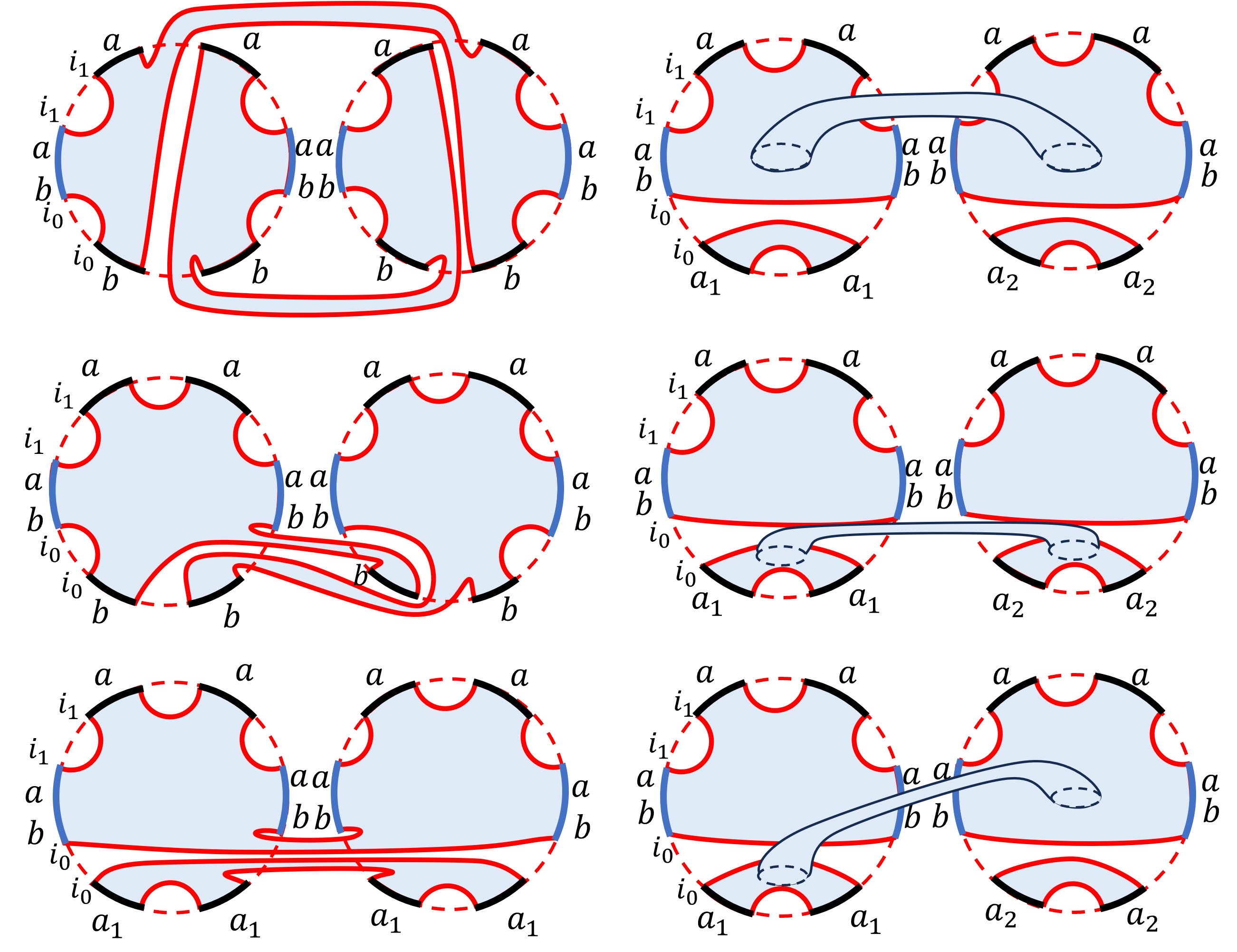
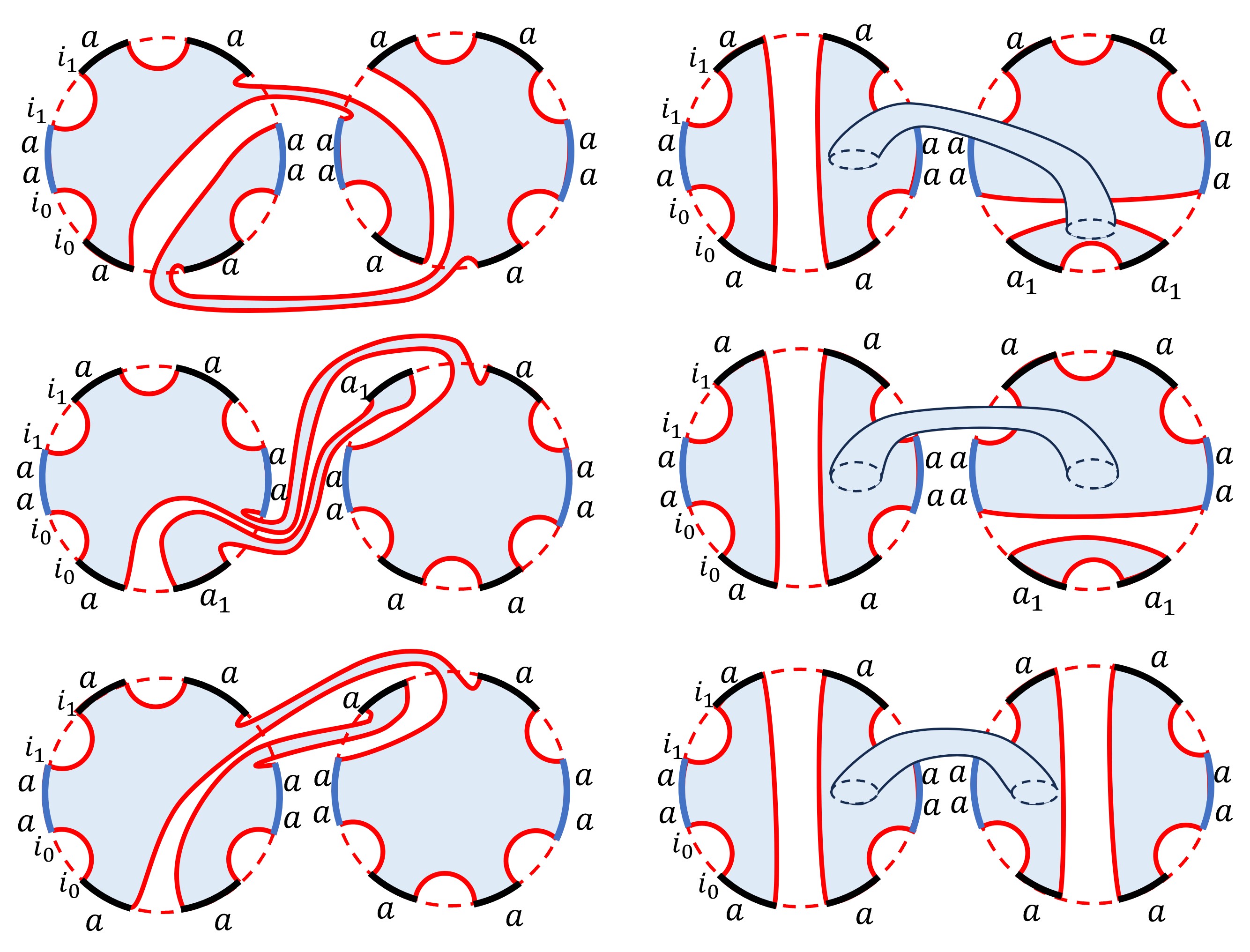
come from wormhole configuration described in Fig 1 for . Summing over these contributions, we obtain
| (4.12) |
We see that when we compare with the relative entropy difference at , the fluctuation is suppressed by . Thus, we conclude that the error in the encoding map has an exponentially suppressed fluctuation, and the approximate recovery map typically exists in the ensemble.
4.3 Entanglement Fidelity of the Petz Recovery Map
Next, we study the entanglement fidelity of the Petz map and examine possible errors in the recovery map. We first consider general quantum state on the code subspace. Before considering the entanglement fidelity, it is convenient to study the following amplitude
It is clear that when this always gives , the Petz map is an exact recovery map. In the case of the PSSY model, the encoding map has symmetry on average; thus we can write
| (4.14) |
Then, the exact recovery is equivalent to . Since the composite map is trace-preserving, we generally have . To evaluate and , we can use the standard replica trick
| (4.15) | |||||
and take the limit . Then, at large and , we have Penington:ReplicaWormholeWestCoast
| (4.16) |
Thus at , we have annd . This means that the Petz map is an approximate recovery map on average.
We now consider the entanglement fidelity. For a diagonal density matrix , the entanglement fidelity of the channel is given by
| (4.17) | |||||
here is the purification of . At , we have
| (4.18) |
In the following, we will consider the fluctuation of this entanglement fidelity.
Fluctuation in the Entanglement Fidelity of the Petz Map
In order to evaluate the fluctuation of the entanglement fidelity, it is useful to evaluate the fluctuation of . We will evaluate
| (4.19) |
Showing both and are small at large implies that the Petz map is indeed an approximate recovery map typically. The wormholes contributing to at are described in Fig 2.
The result is
| (4.21) |
Both and are non-negative for any as they should.
Consider the case when the quantum state is pure . Then, the entanglement fidelity is
| (4.22) |
and its fluctuation is
| (4.23) |
Comparing with the average errors in (4.22), we see that the fluctuation is exponentially suppressed by . Thus, we again conclude that the Petz map is typically an approximate recovery map at .
4.4 Coherent Information Loss
In this subsection, we compute the coherent information loss and compare it with the entanglement fidelity of the Petz map (4.18), using the inequality (2.18). Again, small coherent information loss implies the existence of an approximate recovery map.
Coherent information in the PSSY model was discussed in Balasubramanian:2022fiy . We consider the case when the input density matrix is the maximally mixed state . We deote its purification as . Then the coherent information loss of ad the state is given by
| (4.24) |
We can evaluate this quantity easily by noticing that the second term is the entropy of the Hawking radiation with a replacement , and the third term is also the entropy of the Hawking radiation with a replacement . Then, we can write the coherent information loss explicitly as
| (4.25) |
We see that at , the coherent information loss is small, guaranteeing the existence of an approximate recovery map.
5 Conclusion
In this paper, we examined whether the information recovery from the black hole interior is typically possible in the ensemble of gravitational theories. Both the relative entropy difference and one minus the entanglement fidelity of the Petz map behave as at large on average, which guarantees the existence of an approximate recovery map of the interior information. We have shown that their fluctuations behave as , which is exponentially suppressed by compared to . This implies that information recovery is typically possible in the ensemble of theories.
We note that there are a number of important questions regarding the information recovery from the black hole interior, such as the origin of the ensemble averaging in quantum gravity. We have also not answered all the questions about the fluctuation of the recovery measures. We have essentially limited to the case of pure quantum state as the interior information. To evaluate the fluctuations for a more general input state, one needs to compute in the case of the entanglement fidelity. We have only considered the maximally mixed state in the coherent information. It would be interesting to consider more general input states, as well as the fluctuations of the coherent information loss. We expect the fluctuations of these measures are similarly suppressed by compared to the signal, while detailed studies are required.
It is also interesting that the characterization of the Petz map is under investigation. We note that the Petz map has better properties than the averaged rotated Petz map in terms of retrodiction Parzygnat:2022ldx .
Acknowledgements
We are grateful to F. Buscemi for helpful comments and correspondence. We thank R. Bousso for discussions.
References
- (1) R. Bousso and M. Miyaji, Fluctuations in the Entropy of Hawking Radiation, 2307.13920.
- (2) S. Ryu and T. Takayanagi, Holographic derivation of entanglement entropy from AdS/CFT, Phys. Rev. Lett. 96 (2006) 181602 [hep-th/0603001].
- (3) V.E. Hubeny, M. Rangamani and T. Takayanagi, A Covariant holographic entanglement entropy proposal, JHEP 07 (2007) 062 [0705.0016].
- (4) T. Faulkner, A. Lewkowycz and J. Maldacena, Quantum corrections to holographic entanglement entropy, JHEP 11 (2013) 074 [1307.2892].
- (5) N. Engelhardt and A.C. Wall, Quantum Extremal Surfaces: Holographic Entanglement Entropy beyond the Classical Regime, JHEP 01 (2015) 073 [1408.3203].
- (6) B. Czech, J.L. Karczmarek, F. Nogueira and M. Van Raamsdonk, The Gravity Dual of a Density Matrix, Class. Quant. Grav. 29 (2012) 155009 [1204.1330].
- (7) A. Almheiri, X. Dong and D. Harlow, Bulk Locality and Quantum Error Correction in AdS/CFT, JHEP 04 (2015) 163 [1411.7041].
- (8) F. Pastawski, B. Yoshida, D. Harlow and J. Preskill, Holographic quantum error-correcting codes: Toy models for the bulk/boundary correspondence, JHEP 06 (2015) 149 [1503.06237].
- (9) D.L. Jafferis, A. Lewkowycz, J. Maldacena and S.J. Suh, Relative entropy equals bulk relative entropy, JHEP 06 (2016) 004 [1512.06431].
- (10) X. Dong, D. Harlow and A.C. Wall, Reconstruction of Bulk Operators within the Entanglement Wedge in Gauge-Gravity Duality, Phys. Rev. Lett. 117 (2016) 021601 [1601.05416].
- (11) P. Hayden, S. Nezami, X.-L. Qi, N. Thomas, M. Walter and Z. Yang, Holographic duality from random tensor networks, JHEP 11 (2016) 009 [1601.01694].
- (12) D. Harlow, The Ryu–Takayanagi Formula from Quantum Error Correction, Commun. Math. Phys. 354 (2017) 865 [1607.03901].
- (13) J. Cotler, P. Hayden, G. Penington, G. Salton, B. Swingle and M. Walter, Entanglement Wedge Reconstruction via Universal Recovery Channels, Phys. Rev. X 9 (2019) 031011 [1704.05839].
- (14) C.-F. Chen, G. Penington and G. Salton, Entanglement Wedge Reconstruction using the Petz Map, JHEP 01 (2020) 168 [1902.02844].
- (15) H. Barnum and E. Knill, Reversing quantum dynamics with near-optimal quantum and classical fidelity, Journal of Mathematical Physics 43 (2002) 2097.
- (16) G. Penington, Entanglement Wedge Reconstruction and the Information Paradox, JHEP 09 (2020) 002 [1905.08255].
- (17) A. Almheiri, N. Engelhardt, D. Marolf and H. Maxfield, The entropy of bulk quantum fields and the entanglement wedge of an evaporating black hole, JHEP 12 (2019) 063 [1905.08762].
- (18) A. Almheiri, R. Mahajan, J. Maldacena and Y. Zhao, The Page curve of Hawking radiation from semiclassical geometry, JHEP 03 (2020) 149 [1908.10996].
- (19) G. Penington, S.H. Shenker, D. Stanford and Z. Yang, Replica wormholes and the black hole interior, JHEP 03 (2022) 205 [1911.11977].
- (20) A. Almheiri, T. Hartman, J. Maldacena, E. Shaghoulian and A. Tajdini, Replica Wormholes and the Entropy of Hawking Radiation, JHEP 05 (2020) 013 [1911.12333].
- (21) S. Vardhan, J. Kudler-Flam, H. Shapourian and H. Liu, Mixed-state entanglement and information recovery in thermalized states and evaporating black holes, JHEP 01 (2023) 064 [2112.00020].
- (22) V. Balasubramanian, A. Kar, C. Li and O. Parrikar, Quantum error correction in the black hole interior, JHEP 07 (2023) 189 [2203.01961].
- (23) C. Akers, N. Engelhardt, D. Harlow, G. Penington and S. Vardhan, The black hole interior from non-isometric codes and complexity, 2207.06536.
- (24) B. Czech, S. Shuai and H. Tang, Information recovery in the Hayden-Preskill protocol, 2310.16988.
- (25) Y. Nakayama, A. Miyata and T. Ugajin, The Petz (lite) recovery map for scrambling channel, 2310.18991.
- (26) P. Hayden and J. Preskill, Black holes as mirrors: Quantum information in random subsystems, JHEP 09 (2007) 120 [0708.4025].
- (27) P. Hayden and G. Penington, Learning the Alpha-bits of Black Holes, JHEP 12 (2019) 007 [1807.06041].
- (28) J.M. Maldacena and L. Maoz, Wormholes in AdS, JHEP 02 (2004) 053 [hep-th/0401024].
- (29) P. Saad, S.H. Shenker and D. Stanford, A semiclassical ramp in SYK and in gravity, 1806.06840.
- (30) P. Saad, Late Time Correlation Functions, Baby Universes, and ETH in JT Gravity, 1910.10311.
- (31) D. Harlow and D. Jafferis, The Factorization Problem in Jackiw-Teitelboim Gravity, JHEP 02 (2020) 177 [1804.01081].
- (32) R. Bousso and M. Tomašević, Unitarity From a Smooth Horizon?, Phys. Rev. D 102 (2020) 106019 [1911.06305].
- (33) R. Bousso and E. Wildenhain, Gravity/ensemble duality, Phys. Rev. D 102 (2020) 066005 [2006.16289].
- (34) D. Kretschmann and R.F. Werner, Tema con variazioni: quantum channel capacity, New Journal of Physics 6 (2004) 26.
- (35) F. Buscemi and N. Datta, The quantum capacity of channels with arbitrarily correlated noise, IEEE Transactions on Information Theory 56 (2010) 1447.
- (36) M. Junge, R. Renner, D. Sutter, M.M. Wilde and A. Winter, Universal Recovery Maps and Approximate Sufficiency of Quantum Relative Entropy, Annales Henri Poincare 19 (2018) 2955 [1509.07127].
- (37) B. Schumacher and M.D. Westmoreland, Approximate quantum error correction, Quantum Information Processing 1 (2002) 5.
- (38) F. Buscemi, Entanglement measures and approximate quantum error correction, Phys. Rev. A 77 (2008) 012309.
- (39) F. Buscemi, Irreversibility of entanglement loss, in Theory of Quantum Computation, Communication, and Cryptography, Y. Kawano and M. Mosca, eds., (Berlin, Heidelberg), pp. 16–28, Springer Berlin Heidelberg, 2008.
- (40) C. Teitelboim, Gravitation and Hamiltonian Structure in Two Space-Time Dimensions, Phys. Lett. B 126 (1983) 41.
- (41) R. Jackiw, Lower Dimensional Gravity, Nucl. Phys. B 252 (1985) 343.
- (42) J. Maldacena, D. Stanford and Z. Yang, Conformal symmetry and its breaking in two dimensional Nearly Anti-de-Sitter space, PTEP 2016 (2016) 12C104 [1606.01857].
- (43) D. Stanford and E. Witten, Fermionic Localization of the Schwarzian Theory, JHEP 10 (2017) 008 [1703.04612].
- (44) Z. Yang, The Quantum Gravity Dynamics of Near Extremal Black Holes, JHEP 05 (2019) 205 [1809.08647].
- (45) P. Saad, S.H. Shenker and D. Stanford, JT gravity as a matrix integral, 1903.11115.
- (46) D. Stanford and E. Witten, JT gravity and the ensembles of random matrix theory, Adv. Theor. Math. Phys. 24 (2020) 1475 [1907.03363].
- (47) A.J. Parzygnat and F. Buscemi, Axioms for retrodiction: achieving time-reversal symmetry with a prior, Quantum 7 (2023) 1013 [2210.13531].