Application of some $L_{2}$ optimization to a discrete distribution

Abstract

This paper proposes the novel method to estimate the success probability of the binomial distribution. To that end, we use the Cramer-von Mises type optimization which has been commonly used in estimating parameters of continuous distributions. Upon obtaining the estimator through the proposed method, its desirable properties such as asymptotic distribution and robustness are rigorously investigated. Simulation studies serve to demonstrate that the proposed method compares favorably with other well-celebrated methods including the maximum likelihood estimation.

1 Introduction

The most popular and exoteric random variable (r.v.) among all others would be the binomial r.v. It is used to model the number of occurrence of a binomial outcome – success or failure, 0 or 1, head or tail, etc. – among the fixed number of trials: one textbook example is counting the number of heads when a coin is flipped several times. The binomial probability distribution is governed by a single parameter: the probability of its binary outcome at each trial which is called the success probability. For example, it will be 0.5 in the binomial experiment of flipping a coin and result in a symmetric probability distribution. Unlike the flipping-coin example, the success probability is unknown in many cases: e.g., a free-throw rate of a basketball player. Among many other methods to estimate the success probability, the most famous one is the maximum likelihood (ML) method which yields the ratio of the sample mean to the number of trials as an estimate for the parameter. Since the ML estimator attains the Cramer-Rao lower bound, it is definitely the most efficient among unbiased estimators. However, an issue arises when the binomial distribution is contaminated with a gross error that is introduced in Section 2.3: the ML estimation will lose its efficiency in the presence of the gross error which, in turn, gives a rise to a biased estimator.

The parameter estimation problem of the binomial model – even the contaminated model – has been out of the limelight as mentioned in Ruckstuhl and Welsh (2001). The binomial estimation got the attention from statisticians only when it is extended to the logistic regression model. In all intents and purposes, the colossal amount of attention has been given to the estimation for the logistic regression: see Ruckstuhl and Welsh (2001) and Pregibon (1982). Focusing on the binomial model in its own right, they addressed the issue of the contaminated binomial model and proposed a robust estimation method.

In continuous probability distributions, some methodologies using $L_{2}$ distance functions – which measure a difference between an empirical distribution function obtained from a sample and an assumed distribution function – have been extremely popular for making statistical inferences and estimating parameters. One textbook example of those $L_{2}$ distance functions is the Cramer-von Mises (CvM) type distance. It can be said that the impact of the CvM type distance on the static literature is truly significant: in view of its importance and usage, it is said to be twinned with the Kolmogorov-Smirnov (KS) type distance. In the literature of hypothesis testing, the Anderson-Darling (AD) test based on the CvM type distance has been popular since it was proposed by Anderson and Darling (1952), and its theoretical and computational perspectives have been investigated by many researchers: see, e.g., Marsaglia (2004) and Scholz and Stephens (1987). Razali and Wah (2011) demonstrated the AD test is more powerful than many other tests. The popularity of the CvM type distance was even more prominent in the statistical literature of the parameter estimation. Parr and Schucany (1979) demonstrated practitioner can obtain robust estimators through using CvM type $L_{2}$ distance. Millar (1981, 1982, 1984) proved asymptotic properties of estimators resulting from the CvM type $L_{2}$ distance. Kim (2020) investigated the asymptotic properties of MD estimators of regression parameters when the errors in the regression model are symmetrically distributed but dependent. For more details of desirable properties using the CvM type $L_{2}$ distance, see Koul (2002, p.139) and references therein.

Given that the CvM type distance entails the integration of the density or distribution function, it is no wonder that it doesn’t have any direct or indirect application in the domain of discrete probability distributions. Considering many desirable properties driven by the CvM type distance as mentioned in the previous paragraph, application of its analogue – the continuous measure being replaced with a discrete measure in the distance function – to discrete probability distributions has a good prospect. In this article, application of the analogue of the CvM type distance will be confined to the binomial distribution only. The rest of the article is organized as follows. Section 2.1 will define the estimation problem using the CvM type distance function. Section 2.2 will investigate the asymptotic properties of estimators obtained from the proposed method while Section 2.3 will discuss other properties of the proposed method. Section 3 will compare the proposed method with other well celebrated methods and demonstrate that its superiority.

2 Minimum distance estimation

2.1 Uniformly locally asymptotically quadratic

Consider $X_{1},...,X_{n}$ where $X_{i}$’s are independent and identically distributed (i.i.d.) binomial r.v.  with $m$ and $p_{0}$ being the number of trials and the true success probability for each trial. Let $f$ and $F$ denote probability mass and distribution functions, respectively, that is,

$$f(k;p_{0})=\left(\begin{array}[]{c}m\\ k\end{array}\right)p_{0}^{k}(1-p_{0})^{m-k},\quad F(k;p_{0})=\sum_{j=0}^{k}f(j;p_{0}).$$

Define the distance function for $p\in(0,1)$

$${\cal L}(p)=\sum_{k=0}^{m}\left[\sum_{i=1}^{n}d_{ni}\Big{\{}\mathbf{I}(X_{i}\leq k)-F(k;p)\Big{\}}\right]^{2},$$ (2.1)

where $\mathbf{I}(\cdot)$ is an indicator function and $d_{ni}\in\mathbb{R},\,1\leq i\leq n$ with

$$\sum_{i=1}^{n}d_{ni}^{2}=1,\quad\max_{1\leq i\leq n}d_{ni}^{2}=o(1).$$ (2.2)

Note that any deviation from the true parameter $p_{0}$ is expected to result in larger ${\cal L}$, which are stated in (a.2)–(a.3). In addition, define a sequence of positive real number $\delta_{n}$, tending to infinity as $n$ goes to infinity, and assume that

$$\lim_{n\rightarrow\infty}n\bar{d}_{n}/\delta_{n}=1,$$ (2.3)

where $\bar{d}_{n}:=n^{-1}\sum d_{ni}$: e.g., $d_{ni}=1/\sqrt{n}$ for all $1\leq i\leq n$ with $\delta_{n}=\sqrt{n}$. Subsequently, define the estimator

$${\cal L}(\widehat{p})=\inf_{p\in(0,1)}{\cal L}(p).$$ (2.4)

In the case of continuous r.v.’s, the resulting estimator from minimizing CvM type $L_{2}$ distance is referred to as minimum distance (MD) estimator. Koul (2002) introduced general conditions under which the $L_{2}$ distance function can be approximated by a quadratic function so that the asymptotic distribution of the MD estimator can be derived. He refers to those conditions as uniformly locally asymptotically quadratic (ULAQ) conditions: for more details, see Koul (op.cit, Ch. 5.4). Rigorously exploiting the ULAQ conditions, Kim (2018) proposed the numerical algorithm which solves the MD estimation problem in regression models. As illustrated in the literature including aforementioned works, it transpires that employing the ULAQ conditions is indeed a felicitous idea since they are extremely suitable when the direct estimation is not a viable option for some reasons, especially when the objective function is so complex. Motivated by this fact, we are ready to extend the application of the ULAQ conditions from the parameter estimation of continuous r.v.’s to that of the binomial r.v. Here we introduce the ULAQ conditions specially adapted for the current study.

• There exist a sequence of random variable $S_{n}(p_{0})$ and a sequence of real number $W_{n}(p_{0})$ such that for all $0<b<\infty$

  $$\sup_{|\delta_{n}(p-p_{0})|\leq b}\left|{\cal L}(p)-{\cal L}(p_{0})-(p-p_{0})S_{n}(p_{0})-\frac{1}{2}(p-p_{0})^{2}W_{n}(p_{0})\right|=o_{p}(1).$$

• For all $\varepsilon>0$, there is a $0<z_{\varepsilon}<\infty$ such that

  $$\mathbb{P}\big{(}|{\cal L}(p_{0})|\leq z_{\varepsilon}\big{)}\geq 1-\varepsilon.$$

• For all $\varepsilon>0$ and $0<c<\infty$, there is a $0<b<\infty$ and $N$ – both depending on $\varepsilon$ and $c$ – such that

  $$\mathbb{P}\Big{(}\inf_{\delta_{n}|p-p_{0}|>b}|{\cal L}(p)|>c\Big{)}\geq 1-\varepsilon,\qquad\textrm{ for all }n\geq N.$$

Next, we reproduce Theorem 5.4.1 from Koul (op.cit).

Lemma 2.1.

Suppose (a.1)-(a.3) hold. Then,

$$\delta_{n}(\widehat{p}-p_{0})=\left[\delta_{n}^{-2}W_{n}(p_{0})\right]\left[\delta_{n}^{-1}S_{n}(p_{0})\right]+o_{p}(1).$$

As shown in Lemma 2.1, the successful acquisition of the asymptotic distribution of the binomial MD estimator $\widehat{p}$ hinges on (a.1)-(a.3). Next section will show that these assumptions are indeed met.

2.2 Asymptotic properties of $\widehat{p}$

After ascertaining the ULAQ assumptions (a.1)-(a.3) are met, we proceed to apply Lemma 2.1 and obtain the asymptotic distribution of the binomial MD estimator $\widehat{p}$, which is the main goal of this study; we also compare its asymptotic variance with that of other estimators. Recall that $X_{1},X_{2},...,X_{n}$ are i.i.d.  binomial r.v.  and let $F(\cdot;p)$ be the modelled distribution function. Note that

$$F(k;p) = (m-k)\left(\begin{array}[]{c}m\\ k\end{array}\right)\int_{0}^{1-p}y^{m-k+1}(1-y)^{k}dy,$$

$$= m_{k}\int_{0}^{1-p}g_{k}(y)\,dy,$$

where $m_{k}=(m-k)\left(\begin{array}[]{c}m\\ k\end{array}\right)$ and $g_{k}(y)=y^{m-k+1}(1-y)^{k}$. Using that $x\in\mathbb{R}$

$$(1+x)^{m}=\sum_{k=0}^{m}\left(\begin{array}[]{c}m\\ k\end{array}\right)x^{k},$$

it is easy to see

$$\sum_{k=0}^{m}\{m_{k}\}^{r}<\infty,\quad\textrm{ for }r=1,2.$$ (2.8)

Also, it is by no means clear that

$$\max_{1\leq k\leq n}\sup_{x\in[0,1]}g_{k}(x)=O(1),\quad\lim_{\varepsilon\rightarrow 0}\max_{0\leq k\leq m}\sup_{|x-y|<\varepsilon}|g_{k}(x)-g_{k}(y)|=0.$$ (2.9)

Let $G_{k}(y):=\int_{0}^{y}g_{k}(x)dx$. Observe that

$$F(k;p)-F(k;p_{0})=m_{k}\left[G_{k}(1-p)-G_{k}(1-p_{0})\right].$$ (2.10)

Next, rewrite the distance function

$${\cal L}(p)=\sum_{k=0}^{m}\left[{\cal W}_{d}(k,p)\right]^{2}$$ (2.11)

where

$${\cal W}_{d}(k,p):=\sum_{i=1}^{n}d_{ni}\Big{\{}\mathbf{I}(X_{i}\leq k)-F(k;m,p)\Big{\}}.$$

To obtain the main result of this study, we need to introduce the following equations:

$$S_{n}(p_{0}) = 2n\bar{d}_{n}\sum_{k=0}^{m}{\cal W}_{d}(k,p_{0})m_{k}g_{k}(1-p_{0}),$$

$$W_{n}(p_{0}) = 2n^{2}\bar{d}_{n}^{2}\sum_{k=0}^{m}m_{k}^{2}g_{k}^{2}(1-p_{0}).$$

We shall show that ${\cal L}$ in (2.11) with above $S_{n}$ and $W_{n}$ satisfies the ULAQ conditions (a.1)-(a.3) later. Lemma 2.2 below states that the remaining prerequisites for the asymptotic distribution of the MD estimator – as illustrated in Lemma 2.1 – are satisfied.

Lemma 2.2.

Assume (2.2) and (2.3). Then the following hold true:

• $\delta_{n}^{-1}S_{n}(p_{0})$ is asymptotically normally distributed:

  $$\delta_{n}^{-1}S_{n}(p_{0})\Rightarrow_{{\cal D}}N(0,{\cal C}(p_{0})),$$

  where

  $${\cal C}(p_{0})=\sum_{i=0}^{m}\sum_{j=0}^{m}c_{i}(p_{0})c_{j}(p_{0})\Big{\{}F(i;p_{0})\wedge F(j;p_{0})-F(i;p_{0})F(j;p_{0})\Big{\}}.$$

• There exists $\Gamma(p_{0}):=2\sum_{k=0}^{m}m_{k}^{2}g_{k}^{2}(1-p_{0})$ such that

  $$\lim_{n\rightarrow\infty}\delta_{n}^{-2}W_{n}(p_{0})=\Gamma(p_{0}).$$

Proof.

Convergence of $\delta_{n}^{-2}W_{n}(p_{0})$ directly follows from (2.3). Let $T_{n}:=\{n\bar{d}_{n}\}^{-1}S_{n}(p_{0})$ and $c_{k}(y):=m_{k}g_{k}(1-y)$ for $y\in{\mathbb{R}}$. Rewrite

$$T_{n}=\sum_{k=0}^{m}c_{k}(p_{0}){\cal W}_{d}(k,p_{0})=\sum_{i=1}^{n}d_{ni}\eta_{ni},$$

where

$$\eta_{ni}=\sum_{k=0}^{m}c_{k}(p_{0})\Big{\{}\mathbf{I}(X_{i}\leq k)-F(k;m,p_{0})\Big{\}}.$$

For $a,b\in\mathbb{R}$, let $a\wedge b=\min(a,b)$. Let $\sigma_{k}^{2}:=Var(d_{nk}\xi_{nk})$. A direct calculation shows that

$$\sigma_{k}^{2} = d_{nk}^{2}\sum_{i=0}^{m}\sum_{j=0}^{m}c_{i}(p_{0})c_{j}(p_{0})\Big{\{}F(i;p_{0})\wedge F(j;p_{0})-F(i;p_{0})F(j;p_{0})\Big{\}}$$

$$= d_{nk}^{2}{\cal C}(p_{0}),\quad\quad say.$$

Let $s_{n}^{2}:=\sum_{k=1}^{n}\sigma_{k}^{2}$. The first assumption in (2.2) implies $s_{n}^{2}={\cal C}(p_{0})$. Note that

$$|\eta_{ni}|\leq\sum_{k=0}^{m}|c_{k}(p_{0})|<\infty.$$

Thus, for any $\varepsilon>0$

$$s_{n}^{-2}\sum_{k=1}^{n}d_{nk}^{2}\mathbb{E}\left[\eta_{nk}^{2}:d_{nk}|\eta_{nk}|\geq\varepsilon s_{n}\right] \leq C_{1}s_{n}^{-2}\max_{1\leq i\leq n}d_{ni}^{2}\sum_{k=1}^{n}\mathbb{P}(d_{nk}|\eta_{nk}|\geq\varepsilon s_{n})$$

$$\leq C_{2}s_{n}^{-4}\varepsilon^{-2}\max_{1\leq i\leq n}d_{ni}^{2}\longrightarrow 0,$$

where $C_{1},\,\,C_{2}$ are real values, and the second inequality follows from (2.2) after application of the Chevyshev inequality while the convergence to 0 is the immediate result of the $o(1)$ assumption in (2.2). Finally, application of the Lindeberg-Feller central limit theorem yields

$$T_{n}\Rightarrow_{{\cal D}}N(0,{\cal C}(p_{0})),$$

which, from (2.3), implies $\delta_{n}^{-1}S_{n}(p_{0})$ asymptotically follows a normal distribution with the same asymptotic variance ${\cal C}(p_{0})$. ∎

The remaining task is to demonstrate that the ULAQ conditions are satisfied. Theorem 2.1 verifies (a.1) and is consecutively followed by Lemma 2.3 showing that (a.2) and (a.3) hold.

Theorem 2.1.

Assume (2.2) and (2.3). Then, the distance function ${\cal L}$ in (2.1) satisfies (a.1), that is, for any $0<b<\infty$,

$$\mathbb{E}\sup_{|\delta_{n}(p-p_{0})|\leq b}|{\cal L}(p)-{\cal Q}(p)|=o(1),$$

where

$${\cal Q}(p)={\cal L}(p_{0})+(p-p_{0})S_{n}(p_{0})+\frac{1}{2}(p-p_{0})^{2}W_{n}(p_{0}).$$

Proof.

Recall ${\cal L}(p_{0})=\sum_{k=0}^{m}\left[{\cal W}_{d}(k,p_{0})\right]^{2}$. Rewrite

$${\cal L}(p)=\sum_{k=0}^{m}\left[{\cal W}(k,p_{0})-n\bar{d}_{n}\{F(k;p)-F(k;p_{0})\}\right]^{2},$$

and

$${\cal Q}(p)=\sum_{k=0}^{m}\left[{\cal W}(k,p_{0})+(p-p_{0})n\bar{d}_{n}m_{k}g_{k}(1-p_{0})\right]^{2}.$$

Let $F(\cdot)$ and $F_{0}(\cdot)$ denote $F(\cdot;p)$ and $F(\cdot;p_{0})$, respectively, to conserve the space. Expansion of the summands of ${\cal L}$ and ${\cal Q}$ and subsequent application of the C-S and Minkowski inequalities to the cross product term yields

$$|{\cal L}(p)-{\cal Q}(p)| \leq \sum_{k=0}^{m}\left[n\bar{d}_{n}\{F(k)-F_{0}(k)+(p-p_{0})m_{k}g_{k}(1-p_{0})\}\right]^{2}$$

$$\,\,+2\left[\sum_{k=0}^{m}(n\bar{d}_{n})^{2}\{F(k)-F_{0}(k)+(p-p_{0})m_{k}g_{k}(1-p_{0})\}^{2}\right]^{1/2}$$

$$\,\,\times\left(\left[\sum_{k=0}^{m}\{{\cal W}(k,p_{0})\}^{2}\right]^{1/2}+\left[\sum_{k=0}^{m}\{(p-p_{0})n\bar{d}_{n}m_{k}g_{k}(1-p_{0})\}^{2}\right]^{1/2}\right).$$

Let $u:=\delta_{n}(p-p_{0})$. To prove the theorem, it suffices to show that $E\sum_{k=0}^{m}[{\cal W}_{d}(k,p_{0})]^{2}=O(1)$,

$$\sup_{|u|\leq b}\sum_{k=0}^{m}\Big{[}u\delta_{n}^{-1}n\bar{d}_{n}m_{k}g_{k}(1-p_{0})\Big{]}^{2}=O(1),$$

and

$$\sup_{|u|\leq b}\sum_{k=0}^{m}\Big{[}n\bar{d}_{n}\big{\{}F(k)-F_{0}(k)+u\delta_{n}^{-1}m_{k}g_{k}(1-p_{0})\big{\}}\Big{]}^{2}=o(1).$$

Observe that the first claim follows from the assumption $\sum_{i=1}^{n}d_{ni}^{2}=O(1)$. The supremand of the second claim is bounded by

$$b^{2}(n\bar{d}_{n}/\delta_{n})^{2}\left[\max_{1\leq k\leq n}\sup_{x\in[0,1]}g_{k}(x)\right]^{2}\sum_{k=0}^{m}m_{k}^{2}=O(1),$$

where $O(1)$ follows from $(\ref{eq:del})$ and $(\ref{eq:mk})$, thereby completing the proof of the second claim. Define

$$\xi_{u}:=\sum_{k=0}^{m}\left[n\bar{d}_{n}\{F(k)-F_{0}(k)+u\delta_{n}m_{k}g_{k}(1-p_{0})\}\right]^{2}.$$

Observe that for $|u|\leq b$

$$\Big{|}n\bar{d}_{n}\{F(k)-F_{0}(k)+u\delta_{n}m_{k}g_{k}(1-p_{0})\}\Big{|}\leq b(n\bar{d}_{n}/\delta_{n})\left[\sum_{k=0}^{m}m_{k}\right]\left[\max_{0\leq k\leq m}\sup_{|x-y|<b\delta_{n}^{-1}}|g_{k}(x)-g_{k}(y)|\right].$$

Thus, the third claim follows from (2.3), (2.8), and (2.9), thereby completing the proof of the theorem. ∎

For any function $h:\mathbb{R}\rightarrow\mathbb{R}$, define $\|h\|_{m}^{2}:=\sum_{k=0}^{m}\{h(k)\}^{2}$. Let ${\cal F}:=\sum_{k=0}^{m}{\cal F}_{k}$ with ${\cal F}_{k}:=F_{0}(k)(1-F_{0}(k))$.

Lemma 2.3.

Suppose the assumptions of Theorem 2.1 hold. Then, (a.2)-(a.3) holds.

Proof.

Note that $E|{\cal L}(p_{0})|={\cal F}$. Thus a choice of $z_{\varepsilon}>{\cal F}/\varepsilon$ for the given $\varepsilon>0$ will satisfy (a.2) by the Chebyshev inequality. Define $\ell(p_{0}):=\sum_{k=0}^{m}{\cal W}_{d}(k,p_{0})f_{0}(k)$ and $V_{n}(u):=\sum_{k=0}^{m}{\cal W}_{d}(k,p_{n})f_{0}(k)$ where $f_{0}$ is the first derivative of $F_{0}$. Application of the C-S inequality to $\ell(p_{0})$ yields

$$E|\ell(p_{0})|\leq\|f_{0}\|_{m}{\cal F}^{1/2}.$$

Thus, subsequent application of the Chevyshev inequality to $\ell(p_{0})$ implies that there is $a_{\varepsilon}$ such that

$$\mathbb{P}(|\ell(p_{0})|\leq a_{\varepsilon})\geq 1-\varepsilon.$$ (2.12)

Next, another application of the C-S inequality to $V_{n}(u)$ yields that

$$\inf_{|u|\geq b}|{\cal L}(p)|\geq\inf_{|u|\geq b}|V_{n}(u)|^{2}/\|f_{0}\|_{m}^{2}.$$

To complete the proof of the lemma, it, thus, suffices to show that for every $\epsilon>0$ and $0<c<\infty$, there exists $N_{\epsilon}$ such that

$$\mathbb{P}\Big{(}\inf_{|u|\geq b}|V_{n}(u)|^{2}/\|f_{0}\|_{m}^{2}\geq c\Big{)}\geq 1-\epsilon,\textrm{ for all }n\geq N_{\epsilon}.$$

Define

$$\widetilde{V}_{n}(u):=l(p_{0})+u(\delta_{n}^{-1}n\bar{d}_{n})\sum_{k=0}^{m}m_{k}g_{k}(1-p_{0})f_{0}(k).$$

Note that $|\widetilde{V}_{n}(u)|^{2}$ is quadratic in $u$, rendering the problem to find the infimum over $|u|\geq b$ easier. Therefore, we shall show that there doesn’t exist too much difference between $V_{n}(u)$ and $\widetilde{V}_{n}(u)$, i.e.,

$$\sup_{|u|\leq b}|V_{n}(u)-\widetilde{V}_{n}(u)|=o_{p}(1).$$ (2.13)

By the C-S inequality, we have

$$\mathbb{E}\sup_{|u|\leq b}|V_{n}(u)-\widetilde{V}_{n}(u)|^{2}\leq\|f_{0}\|_{m}^{2}\mathbb{E}\left(\sup_{|u|\leq b}\sum_{k=0}^{m}\left[n\bar{d}_{n}\{F(k)-F_{0}(k)+u\delta_{n}m_{k}g_{k}(1-p_{0})\}\right]^{2}\right),$$

and hence, (2.13) again follows from (2.3), (2.8), and (2.9). Let $\kappa_{n}:=(\delta_{n}^{-1}n\bar{d}_{n})\sum_{k=0}^{m}m_{k}g_{k}(1-p_{0})f_{0}(k)\geq 0$ and $\kappa:=\frac{1}{2}\liminf\kappa_{n}$. Thus, there exists $N_{\kappa}$ such that for all $n\geq N_{\kappa}$, $\kappa_{n}\geq\kappa$. Recall $a_{\varepsilon}$ in (2.12). Next, for any $0<c<\infty$, choose $b$ such that

$$b\geq(a_{\varepsilon/2}+c^{1/2}\|f_{0}\|_{m})/\kappa.$$ (2.14)

Then, we have

$$\mathbb{P}\Big{(}\inf_{|u|\geq b}|\widetilde{V}_{n}(u)|^{2}/\|f_{0}\|_{m}^{2}\geq c\Big{)} = \mathbb{P}\Big{(}|\widetilde{V}_{n}(b)|^{2}/\|f_{0}\|_{m}^{2}\geq c\Big{)}$$

$$\geq \mathbb{P}\Big{(}|\widetilde{V}_{n}(b)|\geq c^{1/2}\|f_{0}\|_{m}\Big{)}$$

$$\geq \mathbb{P}\Big{(}\big{|}|\ell(p_{0})|-b|\kappa_{n}|\big{|}\geq c^{1/2}\|f_{0}\|_{m}\Big{)}$$

$$\geq \mathbb{P}\Big{(}|\ell(p_{0})|\leq b|\kappa_{n}|-c^{1/2}\|f_{0}\|_{m}\Big{)}$$

$$\geq \mathbb{P}\Big{(}|\ell(p_{0})|\leq b\kappa-c^{1/2}\|f_{0}\|_{m}\Big{)}\qquad\textrm{ for all }n\geq N_{\kappa},$$

$$\geq \mathbb{P}\Big{(}|\ell(p_{0})|\leq a_{\varepsilon/2}\Big{)}\,\,\,\qquad\qquad\qquad\textrm{ for all }n\geq N_{\kappa},$$

$$\geq 1-\varepsilon/2\quad\qquad\qquad\qquad\qquad\qquad\textrm{ for all }n\geq N_{\kappa},$$

where the the first equality follows from the quadraticity of $|\widetilde{V}_{n}(u)|^{2}$ in $u$, the second inequality follows from $\big{|}d_{1}+d_{2}\big{|}\geq\big{|}|d_{1}|-|d_{2}|\big{|}$ for $d_{1},d_{2}\in{\mathbb{R}}$, and the fourth inequality follows from the definition of $\kappa$.

Next, recall

$$V_{n}(u)=\sum_{k=0}^{m}\left[\sum_{i=1}^{n}d_{ni}\left\{\mathbf{I}(X_{i}\leq k)-F(k;p_{0}+\delta_{n}^{-1}u)\right\}\right]f(k),$$

where

$$F(k;p_{0}+\delta_{n}^{-1}u)=m_{k}\int_{0}^{1-p_{0}-\delta_{n}^{-1}u}g_{k}(y)\,dy.$$

Note that $g_{k}>0$ will induce $F(k;p_{0}+\delta_{n}^{-1}u)$ to be non-increasing in $u$, which inversely results in $V_{n}(u)$ being non-decreasing in $u$. Consequently,

$$\mathbb{P}\Big{(}\inf_{|u|\geq b}|V_{n}(u)|^{2}/\|f_{0}\|_{m}^{2}\geq c\Big{)} = \mathbb{P}\Big{(}|V_{n}(b)|^{2}/\|f_{0}\|_{m}^{2}\geq c\Big{)}$$

$$\geq \mathbb{P}\Big{(}|\widetilde{V}_{n}(b)|\geq c^{1/2}\|f_{0}\|_{m}\Big{)}-\varepsilon/2$$

$$\geq 1-\varepsilon,$$

for all $n\geq N_{\kappa}$ where the first inequality follows from $(\ref{eq:Vn})$, thereby completing the proof of the lemma. ∎

We conclude this section by stating the main result of this article.

Theorem 2.2.

Suppose the assumptions of Theorem 2.1 hold. Let $\Gamma(p_{0})$ and ${\cal C}(p_{0})$ be as in Lemma 2.2. Then the MD estimator $\widehat{p}$ in (2.4) will be asymptotically normally distributed, that is,

$$\delta_{n}(\widehat{p}-p_{0})\Rightarrow_{{\cal D}}N(0,\tau(p_{0})),$$

where $\tau(p_{0}):={\cal C}(p_{0})/[\Gamma(p_{0})]^{2}$.

Proof.

Theorem 2.1 and Lemma 2.3 imply the distance function ${\cal L}$ satisfies the ULAQ conditions. Consequently, application of Slutsky’s Theorem to Lemma 2.1 together with Lemma 2.2 completes the proof of the theorem. ∎

Remark 2.1.

Note that the consistency of $\hat{p}$ implies that of $h(\hat{p})$ for any continuous function $h:{\mathbb{R}}\rightarrow{\mathbb{R}}$. For the statistical inference such as a confidence interval, $\tau(p_{0})$ can, therefore, be replaced by $\tau(\hat{p})$ when the necessity to estimate it arises.

2.3 Other properties: efficiency and robustness

Observe that Theorem 2.2 implies that if $\delta_{n}=\sqrt{n}$

$$\lim_{n\rightarrow\infty}nVar(\widehat{p})=\frac{\sum_{i=0}^{m}\sum_{j=0}^{m}c_{i}(p_{0})c_{j}(p_{0})\Big{\{}F_{0}(i\wedge j)-F_{0}(i)F_{0}(j)\Big{\}}}{4\left[\sum_{k=0}^{m}c_{k}(p_{0})\right]^{2}}.$$

Recall the i.i.d.  binomial random sample $X_{1},...,X_{n}$ distributed with $F_{0}$ and let $\bar{X}$ and $\hat{p}_{L}$ denote the sample mean and the ML estimator for $p_{0}$. Note that $\hat{p}_{L}=\bar{X}/m$, and hence, $nVar(\hat{p}_{L})=p_{0}(1-p_{0})/m$. Figure 1 shows the variances of both estimators when the true parameter $p_{0}$ varies from 0.001 to 0.999 with the fixed $m$ (10 or 20).

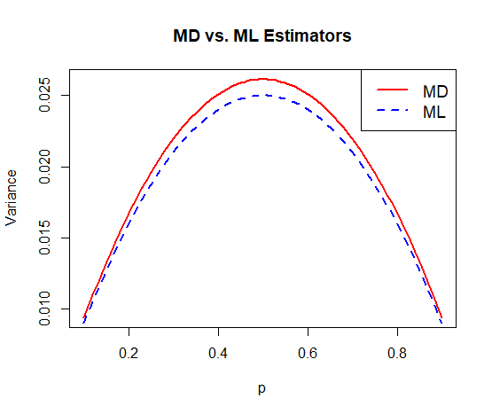
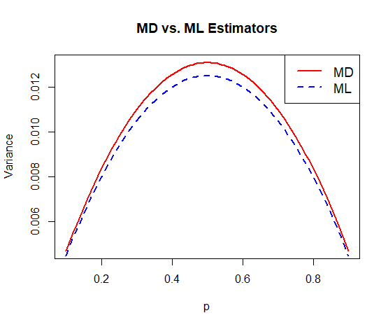
Figure 1: Variances of the MD and ML estimators with $m=10$ (left) or 20 (right).

As illustrated in the figure, the ML estimator always shows smaller variance regardless of $p_{0}$. Both estimators attain the largest variances at $p_{0}=0.5$ while the variances decrease as $p_{0}$ gets away from 0.5. As $m$ increases, the exactly same results hold while both estimators display smaller variances.

Next, consider the following contaminated binomial distribution function

$$F_{\nu}(k)=(1-\nu)F(k)+\nu\zeta_{z},\quad k=0,1,...,m,$$ (2.15)

where $\nu>0$ and $\zeta_{z}$ is a point mass at $z$ with $z\in\{0,1,...,m\}$. To investigate the robustness of estimators, Hampel (1968, 1974) proposed the influence function (IF) which measures how much the gross error $\zeta_{z}$ can influence the estimation itself. Let $\widetilde{p}(F)$ denote the estimator under the assumption of the distribution $F$. Then, IF can be defined as the Gateaux derivative of $\widetilde{p}$ at $F$, that is,

$$IF(z,\widetilde{p},F)=\lim_{\nu\rightarrow 0}\frac{\widetilde{p}(F_{\nu})-\widetilde{p}(F)}{\nu}.$$

It is not difficult to see that

$$IF(z,\hat{p}_{L},F)=\frac{x}{m}-p,$$

which is not bounded, and hence, the ML estimator is not robust since it it not bounded either below or above. To find the IF of the MD estiatmor, let $\widehat{p}_{1}$ denote the MD estimator resulting from using $d_{ni}:=n^{-1/2}$ in (2.1).

Lemma 2.4.

Recall $c_{k}(\cdot)$ and $\Gamma(\cdot)$ in Lemma 2.2. The IF of the MD estimator $\widehat{p}_{1}$ is given by

$$IF(z,\hat{p}_{1},F)=2\Gamma(p)^{-1}\sum_{k=0}^{m}c_{k}(p)\{I(z\leq k)-F(k)\}.$$

Proof.

From $(\ref{eq:rewritten_loss})$ and the asymptotic quadraticity of ${\cal L}$, the MD estimation is equivalent to solving

$$\sum_{k=0}^{m}{\cal W}_{d}(k,p)\,\,\frac{\partial{\cal W}_{d}(k,p)}{\partial p}=0.$$

Therefore, $\partial{\cal W}_{d}(k,p)/\partial p=-\sqrt{n}c_{k}(p)$ implies that the MD estimator satisfies

$$\sum_{i=1}^{n}\phi(X_{i},p)=0,$$

where

$$\phi(y,p)=\sum_{k=0}^{m}c_{k}(p)\Big{\{}I(y\leq k)-F(k;p)\Big{\}}.$$

Then, the similar argument or the direct application of the formula (2.3.5) given in Hampel (1986, p.101) will complete the proof of the lemma.

∎

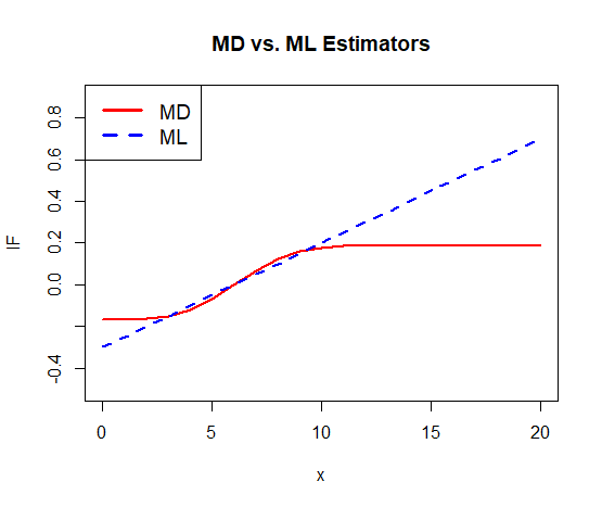
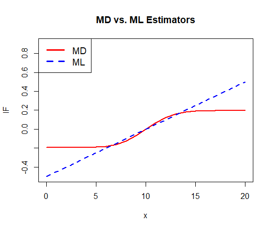
Figure 2: Influence functions of the MD and ML estimators with $m=20$ and $p=0.3$ (left) or 0.5 (right).

As shown in Figure 2, the impact of extreme values on the MD estimator is limited while the same conclusion doesn’t hold for the ML estimator, which is consistent with the previous results.

3 Simulation studies

This section will compare the MD estimator with other well celebrated estimators including the ML estimator through simulated experiments. Ruckstuhl and Welsh (2001) proposed E-estimators which minimizes the likelihood disparity function $H(p,f_{n})$

$$H(p,f_{n})=\sum_{k=0}^{m}\rho_{c_{1},c_{2}}\left(\frac{f_{n}(k)}{f(k;m,p)}\right)f(k;m,p),$$

where $f_{n}$ is an empirical density function and

$$\rho_{c_{1},c_{2}}(x)=\left\{\begin{array}[]{ll}(\log c_{1}+1)x-c_{1},&\hbox{if $x<c_{1}$;}\\ x\log x,&\hbox{if $c_{1}\leq x\leq c_{2}$;}\\ (\log c_{2}+1)x-c_{2},&\hbox{if $x>c_{2}$.}\end{array}\right.$$

Using various combinations of $c_{1}$ and $c_{2}$, they showed E- estimators are more robust than any other estimators including the ML estimator.

Together with the true binomial distribution $F$, we will consider the contaminated binomial distribution $F_{\nu}$ in (2.15) for the following studies. According to $F$ or $F_{\nu}$, we will generate a random sample of $X_{1},...,X_{n}$ with $n$ varying from 20 to 100. Upon the generation, the MD, ML and E-estimators will be computed. Next, we iterate this process 10,000 times. Finally, the bias, standard error (SE), and root mean squared error (RMSE) of three methods will be computed from the 10,000 estimates.

3.1 Estimation under the true distribution

Tables below report results of the simulation experiment when the random sample is generated by the true distribution $F$ with $m=10$ or 20 and $p=0.3$. For other pairs of $m$ and $p$, the almost same result is shown, and hence, we do not report here; the same applies to the contaminated model in the following section.

	MD			ML			E
$n$	Bias	SE	RMSE	Bias	SE	RMSE	Bias	SE	RMSE
20	-8e-04	0.001	0.0323	-2e-04	0.001	0.0313	7e-04	0.0014	0.0373
40	0.001	5e-04	0.023	0.002	5e-04	0.0226	0.0025	7e-04	0.0269
60	-8e-04	4e-04	0.0194	1e-04	4e-04	0.0189	0.001	5e-04	0.0218
80	-5e-04	3e-04	0.0161	4e-04	2e-04	0.0157	0.0012	3e-04	0.0185
100	-0.001	2e-04	0.015	$<$1e-04	2e-04	0.0148	9e-04	3e-04	0.017

Table 1: Bias, SE, and RMSE of the three estimators for $F$ with $m=10$

Table 1 reports the bias, SE and RMSE of the MD, ML, and E-estimators when $m=10$. As shown in the table, the ML estimator outperforms the other two for all three measures.

	MD			ML			E
$n$	Bias	SE	RMSE	Bias	SE	RMSE	Bias	SE	RMSE
20	-0.0012	5e-04	0.0219	-2e-04	5e-04	0.0215	-6e-04	7e-04	0.0271
40	-9e-04	3e-04	0.0166	-1e-04	3e-04	0.0164	1e-04	4e-04	0.0194
60	-9e-04	2e-04	0.0135	2e-04	2e-04	0.0132	-2e-04	2e-04	0.0158
80	-0.0012	1e-04	0.0118	-2e-04	1e-04	0.0115	-2e-04	2e-04	0.0139
100	-0.0017	1e-04	0.0104	-6e-04	1e-04	0.0101	-0.001	1e-04	0.012

Table 2: Bias, SE, and RMSE of estimators for $F$ with $m=20$.

The result of $m=20$ is reported in Table 2, which again shows the same conclusion holds. Thus, it is not rash to conclude that the ML method is superior to the other two methods under no existence of the gross error.

3.2 Estimation under the contaminated distribution

When generating a random sample from the contaminated distribution $F_{\nu}$, we set $\nu$ and $z$ at 0.01 and $m$, respectively. Like the previous section, Tables 3 and 4 report results corresponding to $m=10$ and 20, respectively, with $p$ being fixed at 0.3 but $n$ varying. Consider the case of $m=10$ first.

	MD			ML			E
$n$	Bias	SE	RMSE	Bias	SE	RMSE	Bias	SE	RMSE
20	7e-04	0.0012	0.035	0.0058	0.0013	0.0371	-0.0011	0.0017	0.0407
40	7e-04	6e-04	0.0239	0.0061	6e-04	0.0258	-8e-04	7e-04	0.027
60	0.002	4e-04	0.0191	0.0072	4e-04	0.0212	0.0012	5e-04	0.0214
80	0.0022	3e-04	0.0168	0.0075	3e-04	0.0192	0.0019	3e-04	0.0184
100	0.0014	2e-04	0.0151	0.0066	3e-04	0.0173	8e-04	3e-04	0.0166

Table 3: Bias, SE, and RMSE of the three estimators for $F_{\nu}$ with $m=10$.

A quick glance reveals that the results reported in the tables show a stark difference when compared those reported in the previous section: unlike the true distribution case, the ML estimator doesn’t show a superiority any more. Instead, the MD estimator shows the smallest RMSE consequential upon the smallest SE while the E-estimator shows the smallest bias regardless of $n$; the smallest bias accomplished by the E-estimator also accords with the result reported in Ruckstuhl and Welshi (2001). When the comparison is confined to the MD and ML methods only, the MD method dominates the ML method in terms of all measure; the MD method shows much smaller bias – being also consistent with Figure 2 – and slightly smaller or the same SE, both of which result in smaller RMSE. More precisely, the ML estimator displays from five ($n=100$) to eight ($n=20$) times larger bias than the MD estimator.

	MD			ML			E
$n$	Bias	SE	RMSE	Bias	SE	RMSE	Bias	SE	RMSE
20	2e-04	6e-04	0.0238	0.0056	7e-04	0.0278	-0.0016	8e-04	0.0277
40	9e-04	3e-04	0.0165	0.0074	4e-04	0.0205	-6e-04	4e-04	0.0194
60	0.001	2e-04	0.0139	0.0071	3e-04	0.0178	-3e-04	2e-04	0.0157
80	6e-04	1e-04	0.0115	0.0067	2e-04	0.015	-6e-04	2e-04	0.0131
100	7e-04	1e-04	0.0106	0.0067	1e-04	0.0138	-2e-04	1e-04	0.012

Table 4: Bias, SE, and RMSE of the three estimators for $F_{\nu}$ with $m=20$.

Table 4 reports the result corresponding to $m=20$. Even though there is a difference in the degree of extent, the result in Table 4 shows more or less the same modality as the previous result in Table 3: the MD estimator shows the smallest SE and RMSE while the E-estimator shows the smallest bias. Wrapping up all the results from Tables 3 and 4, we conclude the MD estimator outperforms the ML estimator by all measure and the E-estimator by the SE and RMSE.

4 Conclusion

In this study, we extended the application of the CvM type distance – which is popular in the continuous probability distributions – to a binomial distribution and proposed the MD estimator of the binomial success probability $p$ through using its analogue, that is, with the integral of the original CvM type distance being replaced by the summation. Based on the promising results shown in this article, further extension to broad range of discrete probability distributions and and to other statistical model such as the logistic regression is expected to yield some desirable results, and hence, will form future research.

References

- [1] Anderson, T. W. and Darling, D. A. (1952). Asymptotic theory of certain ”goodness-of-fit” criteria based on stochastic processes. Ann. Math. Stat., 23 (2) 193-212.
- [2] Kim, J. (2018). A fast algorithm for the coordinate-wise minimum distance estimation. Comput. Stat., 88 (3) 482-497.
- [3] Kim, J. (2020). Minimum distance estimation in linear regression with strong mixing errors. Commun. Stat.-Theory Methods., 49 (6) 1475-1494.
- [4] Koul, H. L. (2002). Weighted empirical process in nonlinear dynamic models. Springer, Berlin, Vol. 166.
- [5] Marsaglia, G. (2004). Evaluating the Anderson-Darling Distribution. J. Stat. Softw., 9(2) 730-737.
- [6] Millar, P. W. (1981). Robust estimation via minimum distance methods. Zeit fur Wahrscheinlichkeitstheorie., 55 73-89.
- [7] Millar, P. W. (1982). Optimal estimation of a general regr ession function. Ann. Statist., 10, 717-740 .
- [8] Millar, P. W. (1984). A general approach to the optimality of minimum distance estimators. Trans. Amer. Math. Soc., 286 377-418
- [9] Parr, W. C. and Schucany, W. R. (1979). Minimum distance and robust estimation. J. Amer. Statist. Assoc., 75 616-624.
- [10] Ruckstuhl, A. F. and Welshi, A. H. (2001). Robust fitting of the binomial model. Ann. Statist., 29(4) 1117-1136.
- [11] Razali, N. and Wah, Y. B. (2011). Power comparisons of Shapiro–Wilk, Kolmogorov–Smirnov, Lilliefors and Anderson–Darling tests. J. Stat. Model. Anal., 2 (1): 21–33.
- [12] Scholz, F. W. and Stephens, M. A. (1987). K-sample Anderson–Darling Tests. J. Am. Stat. Assoc., 82 (399): 918–924.