Solvable limit of ETH matrix model for double-scaled SYK

Abstract

We study the two-matrix model for double-scaled SYK model, called ETH matrix model introduced by Jafferis et al [arXiv:2209.02131]. If we set the parameters $q_{A},q_{B}$ of this model to zero, the potential of this two-matrix model is given by the Gaussian terms and the $q$-commutator squared interaction. We find that this model is solvable in the large $N$ limit and we explicitly construct the planar one- and two-point function of resolvents in terms of elliptic functions.

1 Introduction

Sachdev-Ye-Kitaev (SYK) model is a very useful toy model for the study of quantum gravity Sachdev1993 ; Kitaev1 ; Kitaev2 ; Polchinski:2016xgd ; Maldacena:2016hyu . At low energy, SYK model is described by the Schwarzian mode which is holographically dual to the Jackiw-Teitelboim (JT) gravity Jackiw:1984je ; Teitelboim:1983ux . In the seminal paper Saad:2019lba , it was found that JT gravity is equivalent to a random matrix model in the double scaling limit.

One can go beyond the low energy Schwarzian approximation by taking a certain double scaling limit of the SYK model Cotler:2016fpe ; Berkooz:2018jqr , which we will call double-scaled SYK (DSSYK) in this paper. As shown in Berkooz:2018jqr , DSSYK is exactly solvable in the large $N$ limit using the technique of the chord diagram and the transfer matrix. One can also compute the correlators of matter operator $\mathcal{O}$ in DSSYK using the chord diagram, assuming that the coefficient $K$ in $\mathcal{O}$ and the coefficient $J$ in the Hamiltonian $H$ are independent Gaussian-random variables Berkooz:2018jqr . Thus DSSYK is capable of describing the holographic dual of (a certain $q$-deformation of) JT gravity coupled to a propagating matter field.

As shown in Jafferis:2022wez , the correlators of matter operator $\mathcal{O}$ in DSSYK is written as a two-matrix model with a single trace potential

$$\mathcal{Z}=\int dAdBe^{-N\operatorname{Tr}V(A,B)},$$ (1)

which is called ETH matrix model in Jafferis:2022wez . Here two matrices $A$ and $B$ correspond to $H$ and $\mathcal{O}$, respectively. One can compute the potential $V(A,B)$ as a series expansion in the parameters $q_{A},q_{B}$ of DSSYK by matching the correlators of matter operator $\mathcal{O}$ at the disk level (see (4) and (11) for the definition of the parameters $q_{A},q_{B}$).

If we ignore the effect of matter matrix $B$, the potential for the matrix $A$ can be computed in a closed form Jafferis:2022wez . This one-matrix model for DSSYK reduces to the matrix model of JT gravity Saad:2019lba by zooming in on the edge of the eigenvalue distribution and taking the double scaling limit. Interestingly, the one-matrix model for DSSYK makes sense in the ordinary ’t Hooft expansion without taking the double scaling limit. As shown in Okuyama:2023kdo , the correlators of one-matrix model for DSSYK in this ’t Hooft expansion can be decomposed into the trumpet and the volume of moduli space, in a completely parallel way as the JT gravity matrix model. One important difference from JT gravity is that the bulk geodesic length becomes discrete in DSSYK Jafferis:2022wez ; Lin:2022rbf ; Okuyama:2023kdo ; Okuyama:2023byh .

We are interested in the effect of matter field in the bulk gravity theory. In particular, we would like to understand the loop correction to the wormhole amplitude coming from the matter loop running around the neck of the wormhole. In JT gravity, this loop correction is UV divergent due to the contribution from long, thin wormhole Saad:2019lba ; Penington:2019kki . We expect that DSSYK gives a UV completion of JT gravity coupled to a matter field and the wormhole amplitude computed from the two-matrix model (1) is free of divergence. However, the potential $V(A,B)$ for DSSYK is very complicated and it seems hopeless to solve the two-matrix model (1) even in the planar limit.

It turns out that when $q_{A}=q_{B}=0$, the two-matrix model (1) for DSSYK drastically simplifies and becomes solvable in the large $N$ limit. In this paper, we compute the one- and two-point functions of resolvent $\operatorname{Tr}\frac{1}{\lambda-A}$ in this solvable limit of two-matrix model. In this case, the potential $V(A,B)$ is given by the Gaussian terms together with the $q$-commutator squared interaction (see (20)). It turns out that the matrix $B$ can be integrated out in this case, and the partition function (1) is written as the eigenvalue integral of the matrix $A$. We find that the saddle-point equation for this eigenvalue integral is very similar to the one appeared in the Dijkgraaf-Vafa matrix model of $\beta$-deformed $\mathcal{N}=4$ super Yang-Mills Dijkgraaf:2002dh ; Dorey:2002tj ; Dorey:2002pq and the six vertex model on a random lattice Kostov:1999qx . As a consequence, the planar resolvent of our two-matrix model can be written in terms of an elliptic function, in a similar manner as Dijkgraaf:2002dh ; Dorey:2002tj ; Dorey:2002pq ; Kostov:1999qx . We also find that the two-point function of resolvents is given by the Bergman kernel on a torus. In this computation, it is useful to introduce the ’t Hooft parameter $S$ as in (24). The original matrix model potential (20) corresponds to the $S=1$ case. We find that the planar solution of resolvent behaves differently for $S=1$ and $S<1$.

This paper is organized as follows. In section 2, we review the ETH matrix model of DSSYK defined in Jafferis:2022wez and rewrite it as the eigenvalue integral when $q_{A}=q_{B}=0$. In section 3, we write down the large $N$ saddle-point equation for the resolvent and find a solution which respects the $\mathbb{Z}_{2}$ symmetry $A\to-A$ of the model. In section 4, we compute the two-point function of resolvents in the large $N$ limit. We find that the two-point function is given by the Bergman kernel on a torus. Finally, we conclude in section 5 with some discussion on future problems. In appendix A we compute the even part of the moments of two-point function for $S<1$.

2 Review of ETH matrix model

In this section, we review the ETH matrix model of DSSYK introduced in Jafferis:2022wez .

2.1 Review of DSSYK

SYK model is defined by the Hamiltonian for $M$ Majorana fermions $\psi_{i}~{}(i=1,\cdots,M)$ obeying $\{\psi_{i},\psi_{j}\}=2\delta_{i,j}$ with all-to-all $p$-body interaction

$$H=\mathrm{i}^{p/2}\sum_{1\leq i_{1}<\cdots<i_{p}\leq M}J_{i_{1}\cdots i_{p}}\psi_{i_{1}}\cdots\psi_{i_{p}},$$ (2)

where $J_{i_{1}\cdots i_{p}}$ is a random coupling drawn from the Gaussian distribution with the mean and the variance given by

$$\langle J_{i_{1}\cdots i_{p}}\rangle_{J}=0,\quad\langle J_{i_{1}\cdots i_{p}}^{2}\rangle_{J}=\binom{M}{p}^{-1}.$$ (3)

DSSYK is defined by the scaling limit

$$M,p\to\infty\quad\text{with}\quad q_{A}=e^{-\frac{2p^{2}}{M}}:\text{fixed}.$$ (4)

As shown in Berkooz:2018jqr , the ensemble average of the moment $\operatorname{tr}H^{k}$ reduces to a counting problem of the intersection number of chord diagrams

$$\langle\operatorname{tr}H^{k}\rangle_{J}=\sum_{\text{chord diagrams}}q_{A}^{\#(\text{intersections})}.$$ (5)

Here, $\operatorname{tr}$ in $\operatorname{tr}H^{k}$ refers to the trace over the Fock space of Majorana fermions. Using the technique of the transfer matrix, the disk amplitude $\langle\operatorname{tr}e^{-\beta H}\rangle_{J}$ of DSSYK is explicitly evaluated as Berkooz:2018jqr

$$\langle\operatorname{tr}e^{-\beta H}\rangle_{J}=\int_{0}^{\pi}\frac{d\theta}{2\pi}\mu(\theta)e^{-\beta E(\theta)},$$ (6)

where $\mu(\theta)$ and $E(\theta)$ are given by

$$\mu(\theta)=(q_{A},e^{\pm 2\mathrm{i}\theta};q_{A})_{\infty},\qquad E(\theta)=\frac{2\cos\theta}{\sqrt{1-q_{A}}}.$$ (7)

The $q$-Pochhammer symbol is defined by

$$(a;q)_{\infty}=\prod_{k=0}^{\infty}(1-aq^{k}),$$ (8)

and the measure factor in (7) is a shorthand of

$$(q_{A},e^{\pm 2\mathrm{i}\theta};q_{A})_{\infty} =(q_{A};q_{A})_{\infty}(e^{2\mathrm{i}\theta};q_{A})_{\infty}(e^{-2\mathrm{i}\theta};q_{A})_{\infty}.$$ (9)

One can also introduce a matter field in the bulk which is dual to an operator in DSSYK. One simple example is the length $s$ strings of Majorana fermions

$$\mathcal{O}=\mathrm{i}^{s/2}\sum_{1\leq i_{1}<\cdots<i_{s}\leq M}K_{i_{1}\cdots i_{s}}\psi_{i_{1}}\cdots\psi_{i_{s}}$$ (10)

with Gaussian random coefficients $K_{i_{1}\cdots i_{s}}$ which is drawn independently from the random coupling $J_{i_{1}\cdots i_{p}}$ in the SYK Hamiltonian. The effect of this operator can be made finite by taking the limit $M,s,p\to\infty$ with the following combinations held fixed:

$$\tilde{q}=e^{-\frac{2sp}{M}},\quad q_{B}=e^{-\frac{2s^{2}}{M}}.$$ (11)

In this limit, the random average of the correlator $\operatorname{tr}(e^{-\beta_{2}H}\mathcal{O}e^{-\beta_{1}H}\mathcal{O})$ becomes

$$\langle\operatorname{tr}(e^{-\beta_{2}H}\mathcal{O}e^{-\beta_{1}H}\mathcal{O})\rangle_{J,K}=\int\prod_{i=1,2}\frac{d\theta_{i}}{2\pi}\mu(\theta_{i})e^{-\beta_{i}E(\theta_{i})}\frac{1}{F(\theta_{1},\theta_{2})}$$ (12)

with

$$F(\theta_{1},\theta_{2})=\frac{(\tilde{q}e^{\mathrm{i}(\pm\theta_{1}\pm\theta_{2})};q_{A})_{\infty}}{(\tilde{q}^{2};q_{A})_{\infty}}.$$ (13)

2.2 ETH matrix model of DSSYK

As discussed in Jafferis:2022wez , one can construct a two-matrix model for $N\times N$ matrices $A$ and $B$ which reproduces the disk amplitude (6) and the matter two-point function (12) in the large $N$ limit. The two matrices $A$ and $B$ correspond to $H$ and $\mathcal{O}$ in DSSYK, respectively

$$A\leftrightarrow H,\quad B\leftrightarrow\mathcal{O},$$ (14)

and the size $N$ of the matrices $A,B$ is given by the dimension of the Hilbert space of $M$ Majorana fermions

$$N=2^{M/2}.$$ (15)

As demonstrated in Jafferis:2022wez , one can construct the potential $V(A,B)$ of two-matrix model (1) order by order in the small $(q_{A},q_{B})$ expansion. At the leading order in the small $q_{B}$ expansion, the potential is written as

$$\operatorname{Tr}V(A,B)=\sum_{a=1}^{N}\Bigl{[}V_{0}(\lambda_{a})+V_{\text{ct}}(\lambda_{a})\Bigr{]}+\frac{1}{2}\sum_{a,b=1}^{N}B_{ab}B_{ba}F(\lambda_{a},\lambda_{b})$$ (16)

where we diagonalized the matrix $A$ and denoted the eigenvalue of $A$ as $\{\lambda_{a}\}_{a=1,\cdots,N}$. In the last term of (16), $F(\lambda_{a},\lambda_{b})$ is given by $F(\theta_{a},\theta_{b})$ in (13) with the identification $\lambda_{a}=E(\theta_{a})$. The last term of (16) is constructed in such a way that the propagator of $B$ reproduces the matter two-point function (12) of DSSYK. The first term $V_{0}(\lambda)$ in (16) is determined by requiring that the eigenvalue density $\rho_{0}(\lambda)$ for the matrix $A$ agrees with $\mu(\theta)$ in (7) if we ignore $B$. The second term $V_{\text{ct}}(\lambda)$ in (16) is the counter term introduced so that the one-loop correction coming from integrating out $B$ is canceled and the eigenvalue density $\rho_{0}(\lambda)$ is not modified at the leading order in the large $N$ limit

$$V_{\text{ct}}(\lambda)=-\int d\lambda^{\prime}\rho_{0}(\lambda^{\prime})\log F(\lambda^{\prime},\lambda).$$ (17)

The explicit form of $V_{0}(\lambda)$ and $V_{\text{ct}}(\lambda)$ is given by Jafferis:2022wez

$$V_{0}(\lambda) =\sum_{n=1}^{\infty}(-1)^{n-1}\frac{q_{A}^{\frac{1}{2}n^{2}}}{n}(q_{A}^{\frac{1}{2}n}+q_{A}^{-\frac{1}{2}n})T_{2n}\left(\frac{\sqrt{1-q_{A}}}{2}\lambda\right),$$ (18)

$$V_{\text{ct}}(\lambda) =\sum_{n=1}^{\infty}(-1)^{n}\frac{\tilde{q}^{2n}}{1-q_{A}^{2n}}\frac{q_{A}^{\frac{1}{2}n^{2}}}{n}(q_{A}^{\frac{1}{2}n}+q_{A}^{-\frac{1}{2}n})T_{2n}\left(\frac{\sqrt{1-q_{A}}}{2}\lambda\right),$$

where $T_{n}(\cos\theta)=\cos(n\theta)$ denotes the Chebyshev polynomial of the first kind.

For a general value of $\tilde{q},q_{A}$ and $q_{B}$, it seems hopeless to solve the two-matrix model (1) even in the planar limit. However, it turns out that the two-matrix model becomes solvable in the limit

$$q_{A},q_{B}\to 0,\quad\tilde{q}=\text{finite}.$$ (19)

In this limit (19), the matrix model potential becomes (see eq.(8.52) in Jafferis:2022wez )

$$\operatorname{Tr}V(A,B) =\operatorname{Tr}\left[\frac{1}{2}(1-\tilde{q}^{2})(A^{2}+B^{2})+\frac{\tilde{q}^{2}}{1-\tilde{q}^{2}}A^{2}B^{2}-\frac{\tilde{q}(1+\tilde{q}^{2})}{2(1-\tilde{q}^{2})}ABAB\right]$$ (20)

$$=\frac{1}{2}\operatorname{Tr}\left[(1-\tilde{q}^{2})(A^{2}+B^{2})-\frac{\tilde{q}^{2}}{1-\tilde{q}^{2}}\Bigl{(}[A,B]_{\tilde{q}}\Bigr{)}^{2}\right],$$

where we introduced the $q$-deformed commutator $[A,B]_{\tilde{q}}$ as

$${}_{\tilde{q}}=\tilde{q}^{\frac{1}{2}}AB-\tilde{q}^{-\frac{1}{2}}BA.$$ (21)

This potential (20) is obtained from the $q_{A}\to 0$ limit of (16) since we have already set $q_{B}=0$ in (16). Note that our two-matrix model with the potential (20) is reminiscent of the models appeared in the context of the Dijkgraaf-Vafa model for the $\mathcal{N}=4$ super Yang-Mills with $\beta$-deformation Dijkgraaf:2002dh ; Dorey:2002tj ; Dorey:2002pq ; Rossi:2009mn ; Mansson:2003dm and the six vertex model on a random lattice Kostov:1999qx .

We are interested in the disk and the cylinder amplitude of our model (20) in the large $N$ limit

$$\Bigl{\langle}\operatorname{Tr}e^{-\beta A}\Bigr{\rangle} =N\int d\lambda\rho(\lambda)e^{-\beta\lambda},$$ (22)

$$\Bigl{\langle}\operatorname{Tr}e^{-\beta_{1}A}\operatorname{Tr}e^{-\beta_{2}A}\Bigr{\rangle}_{\text{conn}} =\int d\lambda_{1}d\lambda_{2}\rho(\lambda_{1},\lambda_{2})e^{-\beta_{1}\lambda_{1}-\beta_{2}\lambda_{2}},$$

which are obtained once we know the one- and the two-point function of the resolvent

$$R(\lambda)=\operatorname{Tr}\frac{1}{\lambda-A}.$$ (23)

In order to study this two-matrix model, it is convenient to introduce the ’t Hooft parameter $S$ in the potential (20)

$$\operatorname{Tr}V(A,B)=\frac{1}{2}\operatorname{Tr}\left[(1-\tilde{q}^{2})\Bigl{(}\frac{A^{2}}{S}+B^{2}\Bigr{)}-\frac{\tilde{q}^{2}}{1-\tilde{q}^{2}}\Bigl{(}[A,B]_{\tilde{q}}\Bigr{)}^{2}\right].$$ (24)

As shown in Jafferis:2022wez , this modification of the potential naturally arises when we turn on $q_{A}\neq 0$

$$S=1+\mathcal{O}(q_{A}).$$ (25)

In the rest of this paper, we will study the large $N$ limit of the two-matrix model with the potential in (24). As we will see below, $S=1$ is a somewhat singular limit and setting $S\neq 1$ gives a natural regularization of the model.

3 One-point function of resolvent

In this section, we study the one-point function of resolvent (23) in the large $N$ planar limit.

3.1 Saddle-point equation

One can easily see that $B$ can be integrated out in our two-matrix model since $B$ appears quadratically in the potential $V(A,B)$ in (24). After integrating out $B$, the partition function $\mathcal{Z}$ of two-matrix model (1) is written as the integral over the eigenvalues $\{\lambda_{a}\}_{a=1,\cdots,N}$ of $A$

$$\mathcal{Z} =\int\prod_{a=1}^{N}d\lambda_{a}e^{-\frac{N(1-\tilde{q}^{2})\lambda_{a}^{2}}{2S}}\frac{\prod_{a<b}(\lambda_{a}-\lambda_{b})^{2}}{\prod_{a,b}\sqrt{(1-\tilde{q}^{2})^{2}+\tilde{q}^{2}(\tilde{q}^{\frac{1}{2}}\lambda_{a}-\tilde{q}^{-\frac{1}{2}}\lambda_{b})(\tilde{q}^{-\frac{1}{2}}\lambda_{a}-\tilde{q}^{\frac{1}{2}}\lambda_{b})}}$$ (26)

$$=\int\prod_{a=1}^{N}\frac{d\lambda_{a}e^{-\frac{N(1-\tilde{q}^{2})\lambda_{a}^{2}}{2S}}}{\sqrt{(1+\tilde{q})^{2}-\tilde{q}\lambda_{a}^{2}}}\prod_{a<b}\frac{(\lambda_{a}-\lambda_{b})^{2}}{(1-\tilde{q}^{2})^{2}+\tilde{q}^{2}(\lambda_{a}-\tilde{q}^{-1}\lambda_{b})(\lambda_{a}-\tilde{q}\lambda_{b})}.$$

Here we ignored the overall normalization constant.

We would like to analyze the saddle-point equation for the integral (26) in the large $N$ limit. To this end, it is convenient to make a change of variables

$$\lambda_{a}=2\cosh z_{a}.$$ (27)

Then $\mathcal{Z}$ in (26) is written as

$$\mathcal{Z}=\int\prod_{a=1}^{N}\frac{dz_{a}\sinh z_{a}e^{-\frac{2N}{S}(1-e^{-2\Delta})\cosh^{2}z_{a}}}{\sqrt{\cosh^{2}\Delta-\cosh^{2}z_{a}}}\prod_{a<b}\frac{(\cosh z_{a}-\cosh z_{b})^{2}}{\bigl{(}\cosh(z_{a}+\Delta)-\cosh z_{b}\bigr{)}\bigl{(}\cosh(z_{a}-\Delta)-\cosh z_{b}\bigr{)}},$$ (28)

where $\Delta$ is related to $\tilde{q}$ by

$$\tilde{q}=e^{-\Delta}.$$ (29)

The large $N$ saddle-point equation for the integral (28) is given by

$$4(1-e^{-2\Delta})\cosh z_{a}\sinh z_{a}$$ (30)

$$= \frac{S}{N}\sum_{b\neq a}\left[\frac{2\sinh z_{a}}{\cosh z_{a}-\cosh z_{b}}-\frac{\sinh(z_{a}+\Delta)}{\cosh(z_{a}+\Delta)-\cosh z_{b}}-\frac{\sinh(z_{a}-\Delta)}{\cosh(z_{a}-\Delta)-\cosh z_{b}}\right].$$

Note that the factor $\frac{\sinh z_{a}}{\sqrt{\cosh^{2}\Delta-\cosh^{2}z_{a}}}$ in the integration measure of (28) can be ignored in the saddle-point equation (30) since its effect is sub-leading in the large $N$ limit.

Introducing the one-point function $\omega(z)$ by

$$\omega(z)=\frac{1}{N}\sum_{b=1}^{N}\frac{\sinh z}{\cosh z-\cosh z_{b}},$$ (31)

the saddle-point equation (30) is written as

$$2(1-e^{-2\Delta})\sinh(2z)=S\bigl{[}2\omega(z)-\omega(z+\Delta)-\omega(z-\Delta)\bigr{]}.$$ (32)

If we further define $G(z)$ by

$$G(z)=2e^{-\Delta}\cosh(2z)+S\bigl{[}\omega(z+\Delta/2)-\omega(z-\Delta/2)\bigr{]},$$ (33)

the saddle-point equation (32) implies that $G(z)$ satisfies

$$G(z+\Delta/2)=G(z-\Delta/2).$$ (34)

This is similar to the relation appeared in Dorey:2002pq ; Kostov:1999qx and hence $G(z)$ is solved by an elliptic function, as we will see below.

3.2 Symmetry of $\omega(X)$

We would like to find a solution $G(z)$ to the equation (34) which respects the symmetry of our two-matrix model (24). For this purpose, it is convenient to introduce the variable $X$ as

$$X=e^{z}$$ (35)

and denote $\omega(z)$ and $G(z)$ as $\omega(X)$ and $G(X)$, respectively. From (27), the eigenvalue $\lambda$ and $X$ are related by

$$\lambda=X+X^{-1}.$$ (36)

This is known as the Joukowsky map. Then $G(X)$ in (33) becomes

$$G(X)=\tilde{q}(X^{2}+X^{-2})-S\bigl{[}\omega(\tilde{q}^{\frac{1}{2}}X)-\omega(\tilde{q}^{-\frac{1}{2}}X)\bigr{]},$$ (37)

and $\omega(X)$ in (31) is written as

$$\omega(X)=\frac{1}{N}\left\langle\operatorname{Tr}\frac{X-X^{-1}}{X+X^{-1}-A}\right\rangle.$$ (38)

From this definition, $\omega(X)$ satisfies

$$\omega(X^{-1})=-\omega(X).$$ (39)

Also, from the $\mathbb{Z}_{2}$ symmetry of our two-matrix model (24)

$$A\to-A,$$ (40)

$\omega(X)$ should satisfy

$$\omega(-X)=\omega(X).$$ (41)

From (39), (41), and (34), we find the conditions for $G(X)$

$$G(X)=G(-X)=G(X^{-1})=G(\tilde{q}X).$$ (42)

For later convenience, we introduce the $q$-difference operator $T_{X}$

$$T_{X}f(X)=f(\tilde{q}^{\frac{1}{2}}X)-f(\tilde{q}^{-\frac{1}{2}}X).$$ (43)

Then $G(X)$ in (37) is written as

$$G(X)=\tilde{q}(X^{2}+X^{-2})-ST_{X}\omega(X),$$ (44)

and the saddle-point condition (34) is written as

$$T_{X}G(X)=0.$$ (45)

3.3 Solving the saddle-point equation

As discussed in Kostov:1999qx ; Zakany:2018dio , $G(X)$ obeying the condition (42) can be solved by an elliptic function by introducing the uniformization coordinate $u$ with the standard double periodicity

$$u\sim u+1\sim u+\tau.$$ (46)

One difference from Kostov:1999qx ; Zakany:2018dio is that since $G(X)$ is an even function of $X$ (see the first equality of (42)), the natural variable which is uniformized by $u$ is $X^{2}$, not $X$. Thus we require

$$X^{2}(u+1)=X^{2}(u)=X^{-2}(-u),\quad X^{2}(u+\tau)=X^{2}(u)\tilde{q}^{2},$$ (47)

which is satisfied by

$$X^{2}(u)=\frac{\vartheta_{1}(u_{0}-u)}{\vartheta_{1}(u_{0}+u)},$$ (48)

where $\vartheta_{1}(u)$ is the Jacobi theta function

$$\vartheta_{1}(u)=-\mathrm{i}\sum_{n\in\mathbb{Z}}(-1)^{n}q^{\frac{1}{2}(n+\frac{1}{2})^{2}}e^{2\pi\mathrm{i}u(n+\frac{1}{2})}$$ (49)

with $q=e^{2\pi\mathrm{i}\tau}$. Note that $\vartheta_{1}(u)$ has the properties

$$\vartheta_{1}(u+1)=\vartheta_{1}(-u)=-\vartheta_{1}(u),\quad\vartheta_{1}(u+\tau)=-e^{-\pi\mathrm{i}\tau-2\pi\mathrm{i}u}\vartheta_{1}(u).$$ (50)

Note also that $X^{2}(u)$ in (48) has a zero at $u=u_{0}$ and a pole at $u=-u_{0}$. Using (50), one can show that the last condition in (47) is satisfied by setting $u_{0}$ as

$$e^{2\pi\mathrm{i}u_{0}}=\tilde{q}.$$ (51)

One can easily evaluate the value of $X^{2}(u)$ at several special points

$$X^{2}(0)=1,\quad X^{2}(\pm 1/2)=-1,\quad X^{2}(\pm\tau/2)=-\tilde{q}^{\pm 1},\quad X^{2}(\pm\tau/2\pm 1/2)=-\tilde{q}^{\pm 1}.$$ (52)

From the definition of $G(X)$ in (37), $G(X)$ obeys the boundary condition

$$G(X)\sim\left\{\begin{aligned} &\tilde{q}X^{2}+\mathcal{O}(X^{-2}),&\quad&(X\to\infty),\\ &\tilde{q}X^{-2}+\mathcal{O}(X^{2}),&\quad&(X\to 0).\end{aligned}\right.$$ (53)

Also, from (42) $G(u)=G(X(u))$ should satisfy

$$G(u+1)=G(-u)=G(u+\tau).$$ (54)

One can show that these conditions (53) and (54) are satisfied by the following elliptic function

$$G(X) =-\frac{\tilde{q}\vartheta_{1}(2u_{0})}{\vartheta^{\prime}_{1}(0)}\Biggl{[}\partial_{u}\log X^{2}(u)+\frac{2\vartheta_{1}^{\prime}(2u_{0})}{\vartheta_{1}(2u_{0})}\Biggr{]}.$$ (55)

This is our final result of the one-point function, which implicitly determines $\omega(X)$ via the relation (37). Note that our result guarantees that $G(X)$ is an even function of $X$ since both $G(X)$ in (48) and $X^{2}(u)$ in (48) are expanded around $u=\pm u_{0}$ in the integer powers of $u\mp u_{0}$.

3.4 Period integral

The relation between the ’t Hooft parameter $S$ and the moduli $\tau$ of the torus is fixed by the period integral of $G(X)$. It turns out that the structure of cuts of $G(X)$ is different for $0<S<1$ and $S>1$. Here we focus on the $0<S<1$ case.

In this case, there are two segments in the $u$-plane depicted by the red and blue lines in the figure below:

(56)

which correspond to branch cuts of $G(X)$. The branch points are located at

$$u=\pm u_{b},\pm(\tau-u_{b}),$$ (57)

and $u_{b}$ is determined by the condition Kostov:1999qx

$$\partial_{u}\log X^{2}(u)\Big{|}_{u=u_{b}}=\frac{\vartheta_{1}^{\prime}(u_{b}-u_{0})}{\vartheta_{1}(u_{b}-u_{0})}-\frac{\vartheta_{1}^{\prime}(u_{b}+u_{0})}{\vartheta_{1}(u_{b}+u_{0})}=0.$$ (58)

Let us consider the normalization condition of $G(X)$. Note that $\omega(z)$ in (31) should satisfy

$$\frac{1}{2\pi\mathrm{i}}\oint_{C}dz\omega(z)=\frac{1}{2\pi\mathrm{i}}\oint_{C}\frac{dX}{X}\omega(X)=1,$$ (59)

where $C$ surrounds the cut of $\omega(X)$. This implies that $G(X)$ in (37) satisfies

$$\Pi_{A}=\frac{1}{2\pi\mathrm{i}}\oint_{A}\frac{dX}{X}G(X)=S,$$ (60)

where the $A$-cycle surrounds the lower cut of $G(X)$ (i.e. the blue line of (56)).

We can compute the $A$-period $\Pi_{A}$ by using the technique in Zakany:2018dio and Dorey:2002pq . As shown in Zakany:2018dio , $\Pi_{A}$ is written as

$$\Pi_{A}=\frac{1}{2\pi\mathrm{i}}\frac{\partial}{\partial\tau}\int_{-\frac{1}{2}-\frac{\tau}{2}}^{\frac{1}{2}-\frac{\tau}{2}}duV(\tilde{q}^{\frac{1}{2}}X(u))$$ (61)

where $V(X)$ is the potential for $A$

$$V(X)=\frac{1}{2}(1-\tilde{q}^{2})(X+X^{-1})^{2}.$$ (62)

The integral (61) can be evaluated by using the method in Dorey:2002pq . To this end, it is convenient to introduce

$$f^{2}(u)=-\frac{\vartheta_{4}(u-u_{0})}{\vartheta_{4}(u+u_{0})}$$ (63)

which is related to $X^{2}(u)$ in (48) by

$$f^{2}(u+\tau/2)=\tilde{q}X^{2}(u).$$ (64)

Then $\Pi_{A}$ in (61) is written as

$$\Pi_{A} =\frac{1}{2\pi\mathrm{i}}\frac{\partial}{\partial\tau}\int_{-\frac{1}{2}-\frac{\tau}{2}}^{\frac{1}{2}-\frac{\tau}{2}}duV(f(u+\tau/2))$$ (65)

$$=\frac{1}{2\pi\mathrm{i}}\frac{\partial}{\partial\tau}\int_{-\frac{1}{2}}^{\frac{1}{2}}du^{\prime}V(f(u^{\prime})).$$

From (64), one can show that

$$X^{2}(u-\tau/2)-X^{2}(u+\tau/2) =(\tilde{q}^{-1}-\tilde{q})f^{2}(u),$$ (66)

$$X^{-2}(u-\tau/2)-X^{-2}(u+\tau/2) =(\tilde{q}-\tilde{q}^{-1})f^{-2}(u),$$

and the integral in (65) becomes

$$\Pi_{A} =\frac{1}{2\pi\mathrm{i}}\frac{\partial}{\partial\tau}\int_{-\frac{1}{2}}^{\frac{1}{2}}du\frac{1}{2}(1-\tilde{q}^{2})\Bigl{[}f^{2}(u)+f^{-2}(u)\Bigr{]}$$ (67)

$$=\frac{1}{2\pi\mathrm{i}}\frac{\partial}{\partial\tau}\frac{1}{2}\tilde{q}\int_{-\frac{1}{2}}^{\frac{1}{2}}du\Bigl{[}X^{2}(u-\tau/2)-X^{2}(u+\tau/2)-X^{-2}(u-\tau/2)+X^{-2}(u+\tau/2)\Bigr{]}.$$

As discussed in Dorey:2002pq , this integral is evaluated by taking the residue at $u=\pm u_{0}$

$$\Pi_{A} =\frac{1}{2}\tilde{q}\frac{\partial}{\partial\tau}\Biggl{[}\underset{u=-u_{0}}{\text{Res}}X^{2}(u)-\underset{u=u_{0}}{\text{Res}}X^{-2}(u)\Biggr{]}$$ (68)

$$=\tilde{q}\frac{\partial}{\partial\tau}\frac{\vartheta_{1}(2u_{0})}{\vartheta_{1}^{\prime}(0)}.$$

This is our final result of the $A$-period $\Pi_{A}$. The condition $\Pi_{A}=S$ (60) determines $q=e^{2\pi\mathrm{i}\tau}$ as a function of $\tilde{q}$ and $S$. One can easily show that $\Pi_{A}$ in (68) has the following small $q$ expansion

$$\Pi_{A}=q(-3+\tilde{q}^{-2}+3\tilde{q}^{2}-\tilde{q}^{4})+q^{2}(-18+6\tilde{q}^{-2}+18\tilde{q}^{2}-6\tilde{q}^{4})+\mathcal{O}(q^{3}).$$ (69)

From (69) one can see that the small $q$ regime corresponds to small $\tilde{q}$. Thus we can compute $q$ as a small $\tilde{q}$ expansion with fixed $S$

$$q =S\tilde{q}^{2}+3S(S-1)^{2}\tilde{q}^{4}+3S(S-1)^{2}(9S^{2}-8S+2)\tilde{q}^{6}+\mathcal{O}(\tilde{q}^{8}).$$ (70)

From (70) and (51), $\tau$ and $u_{0}$ are related as

$$\tau\approx 2u_{0}\qquad(\tilde{q}\to 0).$$ (71)

Note also that $\tau$ and $u_{0}$ are pure imaginary when $0<\tilde{q}<1,0<S<1$.

We can also compute $u_{b}$ in the small $\tilde{q}$ expansion by solving the equation for the branch-point (58)

$$e^{2\pi\mathrm{i}u_{b}} =\sqrt{S}(\sqrt{S}-\sqrt{S-1})\tilde{q}\left[1+\frac{1}{2}(S-1)^{3/2}(3\sqrt{S-1}-5\sqrt{S})\tilde{q}^{2}+\mathcal{O}(\tilde{q}^{4})\right].$$ (72)

If we set $S=\cos^{2}\phi$, $u_{b}$ in (72) is expanded as

$$u_{b} =\frac{\tau}{2}+\text{Re}(u_{b}),$$ (73)

$$\text{Re}(u_{b}) =\frac{1}{4\pi}\bigl{[}2\phi-5\tilde{q}^{2}\cos\phi\sin^{3}\phi+\mathcal{O}(\tilde{q}^{4})\bigr{]}.$$

It is also convenient to define

$$X_{b}=X(u_{b})\tilde{q}^{-\frac{1}{2}},\quad\tilde{S}=\left(\frac{X_{b}+X_{b}^{-1}}{2}\right)^{2}.$$ (74)

Then we find that $\tilde{S}$ is expanded as

$$\tilde{S}=S+S(S-1)^{2}\tilde{q}^{2}+S(S-1)^{2}(1-6S+8S^{2})\tilde{q}^{4}+\mathcal{O}(\tilde{q}^{6}).$$ (75)

3.5 Moment of $\omega(X)$

Let us consider the small $X$ expansion of $\omega(X)$ in (38)

$$\omega(X)=-\sum_{n=0}^{\infty}\mu_{n}X^{n}.$$ (76)

From the generating function of the Chebyshev polynomials $T_{n}(t)$

$$\frac{1-X^{2}}{1-2tX+X^{2}}=1+\sum_{n=1}^{\infty}2T_{n}(t)X^{n},$$ (77)

one can see that the coefficient $\mu_{n}$ of this expansion (76) is the expectation value of the moment

$$\mu_{n}=\frac{1}{N}\Bigl{\langle}\operatorname{Tr}\bigl{(}2T_{n}(A/2)\bigr{)}\Bigr{\rangle},\quad(n\geq 1).$$ (78)

Plugging (76) into the definition of $G(X)$ in (37), $G(X)$ is expanded as

$$G(X)=\tilde{q}(X^{2}+X^{-2})+S\sum_{n=1}^{\infty}\mu_{n}(\tilde{q}^{\frac{n}{2}}-\tilde{q}^{-\frac{n}{2}})X^{n}.$$ (79)

We can easily extract the moment $\mu_{n}$ from the expansion of our solution of $G(X)$ (55) around $u=u_{0}$. Our solution (55) guarantees that the odd moments vanish

$$\mu_{2k+1}=0,\quad(k\in\mathbb{Z}_{\geq 0}),$$ (80)

since $G(X)$ in (55) is an even function of $X$ by construction. Thus $G(X)$ is expanded as

$$G(X)=\tilde{q}(X^{2}+X^{-2})+S\sum_{n=1}^{\infty}\mu_{2n}(\tilde{q}^{n}-\tilde{q}^{-n})X^{2n}.$$ (81)

For instance, $\mu_{2}$ and $\mu_{4}$ are obtained from (55) as

$$\mu_{2} =\frac{\tilde{q}}{S(\tilde{q}-\tilde{q}^{-1})}\left[\frac{\vartheta_{1}^{\prime\prime\prime}(0)\vartheta_{1}(2u_{0})^{2}}{2\vartheta_{1}^{\prime}(0)^{3}}+\frac{\vartheta_{1}^{\prime}(2u_{0})^{2}}{\vartheta_{1}^{\prime}(0)^{2}}-\frac{3\vartheta_{1}(2u_{0})\vartheta_{1}^{\prime\prime}(2u_{0})}{2\vartheta_{1}^{\prime}(0)^{2}}-1\right],$$ (82)

$$\mu_{4} =\frac{2\tilde{q}\vartheta_{1}(2u_{0})^{2}}{3S(\tilde{q}^{2}-\tilde{q}^{-2})}\left[\frac{\vartheta_{1}^{\prime\prime\prime}(2u_{0})}{\vartheta_{1}^{\prime}(0)^{3}}-\frac{\vartheta_{1}^{\prime\prime\prime}(0)\vartheta_{1}^{\prime}(2u_{0})}{\vartheta_{1}^{\prime}(0)^{4}}\right].$$

Using the small $\tilde{q}$ expansion of $q$ in (70), we can compute the small $\tilde{q}$ expansion of the moments $\mu_{2n}$

$$\mu_{2} =S-2+S(S-1)^{2}\tilde{q}^{2}+S(S-1)^{2}(6S^{2}-6S+1)\tilde{q}^{4}+\mathcal{O}(\tilde{q}^{6}),$$ (83)

$$\mu_{4} =2(S-1)^{2}+4(S-1)^{3}S\tilde{q}^{2}+2S(S-1)^{2}(14S^{3}-26S^{2}+15S-2)\tilde{q}^{4}+\mathcal{O}(\tilde{q}^{6}),$$

$$\mu_{6} =(-1+S)^{2}(-2+5S)+3(-1+S)^{3}S(-3+5S)\tilde{q}^{2}$$

$$\quad+9(-1+S)^{3}S\left(-1+9S-19S^{2}+13S^{3}\right)\tilde{q}^{4}+\mathcal{O}(\tilde{q}^{6}).$$

One can check that the $\mathcal{O}(\tilde{q}^{0})$ term of $\mu_{2n}$ is equal to

$$\lim_{\tilde{q}\to 0}\mu_{2n}=\int_{-2\sqrt{S}}^{2\sqrt{S}}d\lambda\rho(\lambda)2T_{2n}(\lambda/2),$$ (84)

where $\rho(\lambda)$ is the eigenvalue density of Gaussian one-matrix model with the potential $V(A)=\frac{A^{2}}{2S}$

$$\rho(\lambda)=\frac{\sqrt{4S-\lambda^{2}}}{2\pi S}.$$ (85)

This is expected since in the limit $\tilde{q}\to 0$ the two-matrix model in (24) reduces to two decoupled Gaussian one-matrix models for $A$ and $B$

$$\lim_{\tilde{q}\to 0}\operatorname{Tr}V(A,B)=\operatorname{Tr}\left(\frac{A^{2}}{2S}+\frac{B^{2}}{2}\right).$$ (86)

It turns out that the higher order correction in (83) can be expressed as a deformation of the eigenvalue density

$$\rho(\lambda)=\frac{\sqrt{4\tilde{S}-\lambda^{2}}}{2\pi\tilde{S}}\frac{1+c\lambda^{2}+\mathcal{O}(\lambda^{4})}{1+c\tilde{S}+\cdots},$$ (87)

where $\tilde{S}$ is defined in (75) and $c$ is given by

$$c=-2S(S-1)^{2}\tilde{q}^{4}+\mathcal{O}(\tilde{q}^{6}).$$ (88)

3.6 One-point function at $S=1$

We observe from (83) that the $S\to 1$ limit of the moments is given by

$$\lim_{S\to 1}\mu_{n}=-\delta_{n,2},$$ (89)

which is independent of $\tilde{q}$. This is consistent with the result of Jafferis:2022wez that the planar one-point function of the two-matrix model at $S=1$ remains the same as that of the one-matrix model with the potential $V_{0}(A)$ in (18), which reduces to the Gaussian one-matrix model when $q_{A}=0$

$$\lim_{q_{A}\to 0}V_{0}(A)=T_{2}(A/2)=\frac{A^{2}}{2}-1.$$ (90)

We can explicitly show that the saddle-point condition (42) for $S=1$ is solved by the resolvent of Gaussian one-matrix model with the eigenvalue density

$$\rho(\lambda)=\frac{\sqrt{4-\lambda^{2}}}{2\pi}.$$ (91)

The resolvent (23) for this eigenvalue density is given by

$$R(\lambda)=\int_{-2}^{2}d\lambda^{\prime}\rho(\lambda^{\prime})\frac{1}{\lambda-\lambda^{\prime}}=\frac{1}{2}\bigl{(}\lambda\pm\sqrt{\lambda^{2}-4}\bigr{)}=X^{\pm 1},$$ (92)

where we used the relation between $\lambda$ and $X$ in (36). $X$ and $X^{-1}$ in (92) correspond to different branches of the resolvent. From (92) and the definition of $\omega(X)$ in (38), we find the expansion of $\omega(X)$ around $X=0$ and $X=\infty$

$$\omega(X)=\left\{\begin{aligned} \omega_{0}(X)&=X(X-X^{-1})=X^{2}-1,&\quad&(X\to 0),\\ \omega_{\infty}(X)&=X^{-1}(X-X^{-1})=1-X^{-2},&\quad&(X\to\infty).\end{aligned}\right.$$ (93)

Then we find

$$T_{X}\omega(X) =\omega_{0}(\tilde{q}^{\frac{1}{2}}X)-\omega_{\infty}(\tilde{q}^{-\frac{1}{2}}X)$$ (94)

$$=\tilde{q}(X^{2}+X^{-2})-2,$$

where we assumed

$$\tilde{q}^{\frac{1}{2}}\ll\min\bigl{\{}|X|,|X^{-1}|\bigr{\}}.$$ (95)

Finally, we find that $G(X)$ in (44) for $S=1$ is constant

$$G(X)=\tilde{q}(X^{2}+X^{-2})-T_{X}\omega(X)=2,$$ (96)

which trivially satisfies the saddle-point condition (42).

We should stress that the two-matrix model with the potential (20) itself is not equal to the Gaussian matrix model when $\tilde{q}\neq 0$. We are only claiming that the planar resolvent $\omega(X)$ in (93) for $S=1$ is equal to that of the Gaussian one-matrix model (90), which is expected from the construction of the counter term (17).

3.7 Structure of $u$-plane

From the result of $\Pi_{A}$ in (68), one can show that the condition $\Pi_{A}=S$ for $S=1$ is exactly solved by

$$q=\tilde{q}^{2}.$$ (97)

Namely, $\tau=2u_{0}$ for $S=1$. This is a singular limit since $X(u)$ in (48) becomes an elementary function $X(u)=e^{\pi\mathrm{i}u}$ when $q=\tilde{q}^{2}$. There are no zero and pole for $X(u)=e^{\pi\mathrm{i}u}$. When we take a limit $S\to 1$ from the $S<1$ side, what is happening is that the zero at $u=u_{0}$ and the pole at $u=\tau-u_{0}$ collide as $u_{0}\to\tau/2$ and they pair-annihilate and disappear. Then, the structure of $u$-plane for the $S=1$ case is depicted as

(98)

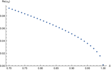
Figure 1: Plot of $\text{Re}(u_{b})$ as a function of $S$ for $\tilde{q}=0.3$.

In Figure 1, we show the plot of $\text{Re}(u_{b})$ computed numerically for $\tilde{q}=0.3$. We can see that $\text{Re}(u_{b})$ vanishes at $S=1$, which implies that the gap around $u=\tau/2$ in (56) closes as $S\to 1$. This is reminiscent of the Gross-Witten transition of unitary matrix model Gross:1980he .

The $u$-plane diagram in (56) is valid for $0<S<1$. We do not have a complete understanding of the solution of $G(X)$ for $S>1$. We can speculate the structure of $u$-plane for $S>1$ by assuming that $X(u)\approx e^{\pi\mathrm{i}u}$ near $S=1$. Then it is natural to define $v$ as

$$v=\frac{1}{\pi\mathrm{i}}\log X=\frac{1}{\pi\mathrm{i}}\log\frac{\lambda+\sqrt{\lambda^{2}-4}}{2},$$ (99)

which is an analogue of the variable $u$. When $S>1$, we expect that the end-point of the cut on the $\lambda$-plane is larger than $2$. In Figure 2, we show the plot of $v$ in (99) for $\lambda\in[-3,3]$. From this behavior, we conjecture that the structure of $u$-plane for $S>1$ looks like this:

(100)

It would be interesting to find the analytic solution of $G(X)$ for $S>1$. We leave this as an interesting future problem.

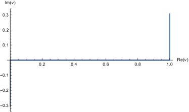
Figure 2: Plot of $v$ in (99) for $\lambda\in[-3,3]$.

4 Two-point function of resolvents

In this section, we study the two-point function of resolvents in our two-matrix model (24). In a similar manner as the one-point function $\omega(X)$ in (38), we define the connected two-point function $\omega(X,Y)$ by

$$\omega(X,Y) =\left\langle\operatorname{Tr}\frac{X-X^{-1}}{X+X^{-1}-A}\operatorname{Tr}\frac{Y-Y^{-1}}{Y+Y^{-1}-A}\right\rangle_{\rm conn}$$ (101)

$$=\left\langle\sum_{a=1}^{N}\frac{X-X^{-1}}{X+X^{-1}-\lambda_{a}}\sum_{b=1}^{N}\frac{Y-Y^{-1}}{Y+Y^{-1}-\lambda_{b}}\right\rangle_{\rm conn}.$$

Our definition of $\omega(X,Y)$ in (101) implies the following symmetry properties:

$$\omega(X,Y)=\omega(Y,X)=-\omega(X^{-1},Y)=\omega(-X,-Y).$$ (102)

Note that $\omega(-X,Y)$ is not equal to $\omega(X,Y)$ in general. Naively, we expect that the structure of cuts of $\omega(X,Y)$ is inherited from that of the one-point function $\omega(X)$. However, this is not the case due to the fact that $\omega(-X,Y)\neq\omega(X,Y)$. We find that only the even part of $\omega(X,Y)$ can be expressed in a simple way for general $S<1$. Interestingly, we find that $S=1$ is special for the two-point function as well. It turns out that when $S=1$ the entire $\omega(X,Y)$ can be constructed in terms of the Bergman kernel on a torus.

4.1 Equation for $\omega(X,Y)$

In this subsection, we derive an equation satisfied by $\omega(X,Y)$. A similar equation is discussed, for example, in Zakany:2018dio .

For this purpose, we need to extend the saddle-point equation (30) to the matrix model with a generic potential for $A$

$$V(X;t)=\sum_{n\in\mathbb{Z}}t_{n}X^{n}.$$ (103)

Here the ’t Hooft parameter $S$ is absorbed into the definition of the parameters $t_{n}$ in the potential $V(X;t)$. The one-point function of this model is given by

$$\omega_{t}(X)=\frac{1}{N}\left\langle\sum_{a=1}^{N}\frac{X-X^{-1}}{X+X^{-1}-X_{a}-X_{a}^{-1}}\right\rangle_{t},$$ (104)

where $X_{a}$ is related to the eigenvalue $\lambda_{a}$ of $A$ by

$$\lambda_{a}\ =\ X_{a}+X_{a}^{-1},$$ (105)

and the average $\langle\cdots\rangle_{t}$ is taken with respect to $V(X;t)$

$$\langle\cdots\rangle_{t}=\frac{1}{\mathcal{Z}_{t}}\int\prod_{a=1}^{N}dz_{a}e^{-NV(e^{z_{a}};t)}(\cdots)\prod_{a<b}\frac{(\cosh z_{a}-\cosh z_{b})^{2}}{\bigl{(}\cosh(z_{a}+\Delta)-\cosh z_{b}\bigr{)}\bigl{(}\cosh(z_{a}-\Delta)-\cosh z_{b}\bigr{)}},$$ (106)

where $\mathcal{Z}_{t}$ is determined by the condition $\langle 1\rangle_{t}=1$. The saddle-point equation for $\omega_{t}(X)$ turns out to be

$$\sum_{n\in\mathbb{Z}}nt_{n}X^{n}=2\omega_{t}(X)-\omega_{t}(\tilde{q}X)-\omega_{t}(\tilde{q}^{-1}X).$$ (107)

From (77), one can show the following identity

$$\frac{Y-Y^{-1}}{Y+Y^{-1}-X-X^{-1}}=-\sum_{n\in\mathbb{Z}}X^{n}Y^{|n|}.$$ (108)

Introducing the so-called loop-insertion operator $D(Y)$ by

$$D(Y)=\sum_{n\in\mathbb{Z}}Y^{|n|}\frac{\partial}{\partial t_{n}},$$ (109)

(108) is written as

$$\frac{Y-Y^{-1}}{Y+Y^{-1}-X-X^{-1}}=-D(Y)V(X;t).$$ (110)

Then, acting $D(Y)$ on $\omega_{t}(X)$ in (104) we find

$$D(Y)\omega_{t}(X)=\omega_{t}(X,Y),$$ (111)

where $\omega_{t}(X,Y)$ is the two-point function defined with respect to $V(X;t)$. Our model of interest corresponds to $t_{n}=t_{n}^{*}$ such that

$$V(X;t^{*})\ =\ \frac{1}{2S}(1-\tilde{q}^{2})(X+X^{-1})^{2},$$ (112)

and we denote $\omega(X)=\omega_{t^{*}}(X)$ and $\omega(X,Y)=\omega_{t^{*}}(X,Y)$. Using the relation (111), one can obtain an equation for $\omega(X,Y)$ by acting the loop-insertion operator $D(Y)$ on both sides of (107) and setting $t_{n}=t_{n}^{*}$. Acting $D(Y)$ on the left-hand side of (107), we find

$$D(Y)\sum_{n\in\mathbb{Z}}nt_{n}X^{n}=-K(X,Y)+K(X,Y^{-1}),$$ (113)

where

$$K(X,Y)=\frac{XY}{(X-Y)^{2}},$$ (114)

and the right-hand side of (107) becomes

$$D(Y)\bigl{[}2\omega_{t}(X)-\omega_{t}(\tilde{q}X)-\omega_{t}(\tilde{q}^{-1}X)\bigr{]}=2\omega_{t}(X,Y)-\omega_{t}(\tilde{q}X,Y)-\omega_{t}(\tilde{q}^{-1}X,Y).$$ (115)

Finally we find the equation for $\omega(X,Y)$

$$-K(X,Y)+K(X,Y^{-1}) =2\omega(X,Y)-\omega(\tilde{q}X,Y)-\omega(\tilde{q}^{-1}X,Y)$$ (116)

$$=-T_{X}^{2}\omega(X,Y),$$

where we define $T_{X}$ and $T_{Y}$ as $q$-difference operators generalizing (43) to the two-variable case

$$T_{X}f(X,Y) =f(\tilde{q}^{\frac{1}{2}}X,Y)-f(\tilde{q}^{-\frac{1}{2}}X,Y),$$ (117)

$$T_{Y}f(X,Y) =f(X,\tilde{q}^{\frac{1}{2}}Y)-f(X,\tilde{q}^{-\frac{1}{2}}Y).$$

Note that the left-hand side of (116) is compatible with the symmetry (102) of $\omega(X,Y)$.

As in the case of one-point function $\omega(X)$, this equation (116) can be simplified by introducing another function $G(X,Y)$ defined by

$$G(X,Y)=T_{X}T_{Y}\omega(X,Y)+K(X,Y)+K(X,Y^{-1}).$$ (118)

From the symmetries of $\omega(X,Y)$ in (102), it follows that $G(X,Y)$ has the symmetries

$$G(X,Y)=G(Y,X)=G(X^{-1},Y)=G(-X,-Y).$$ (119)

Acting $T_{Y}$ on both sides of (116) and using the relation

$$T_{Y}K(X,Y)=-T_{X}K(X,Y),\hskip 14.22636ptT_{Y}K(X,Y^{-1})=T_{X}K(X,Y^{-1}),$$ (120)

we find the equation for $G(X,Y)$

$$T_{X}G(X,Y)=0.$$ (121)

For a fixed $Y$, this equation is the same as (45) for $G(X)$. Therefore, this equation can also be converted to the periodicity condition by employing the conformal transformation $X=X(u)$ and $Y=X(v)$ defined in (48). The function $G(u,v)=G(X(u),X(v))$ then satisfies

$$G(u,v)=G(u+1,v)=G(u+\tau,v).$$ (122)

The same periodicity condition is satisfied for $v$.

However, it turns out that $G(u,v)$ is not an elliptic function of $u$ nor $v$ by the following reason: Note that $G(X,Y)$ is not invariant under $X\to-X$ while $Y$ is kept fixed. From the definition of $X(u)$ in (48), we have

$$X(u)=\sqrt{\frac{\vartheta_{1}(u_{0}-u)}{\vartheta_{1}(u_{0}+u)}}.$$ (123)

One can see that $X(u)$ has square-root branch points at $u=\pm u_{0}$. Thus, the transformation $X\to-X$ is realized by moving $u$ along a closed path encircling $u=u_{0}$ and coming back to the original point on the $u$-plane. The non-invariance of $G(u,v)$ under this transformation then suggests that $G(u,v)$ has an extra branch cut on the $u$-plane, in addition to the ones indicated by the red and blue lines in (56). Therefore, $G(u,v)$ would be rather a function on a Riemann surface of genus-two in general.

It is more convenient to consider the even and the odd parts of $G(X,Y)$ defined by

$$G_{\pm}(X,Y)=\frac{1}{2}\Bigl{[}G(X,Y)\pm G(-X,Y)\Bigr{]}.$$ (124)

Then, the even part $G_{+}(X,Y)$ satisfies $G_{+}(-X,Y)=G_{+}(X,Y)$ and hence it is an elliptic function. All the complications are contained in the odd part $G_{-}(X,Y)$ which we will not discuss in this paper.

When $S=1$, the above problem is curcumvented by the fact that $X(u)=e^{\pi\mathrm{i}u}$ is an entire function on the $u$-plane. As a consequence, the whole $G(X,Y)$ becomes an elliptic function when $S=1$.

4.2 Even part of $G(X,Y)$ for $S<1$

In this subsection, we determine the explicit form of the even part $G_{+}(X,Y)$ for $S<1$. From the definition (118) of $G(X,Y)$ we find

$$G_{+}(X,Y)=\frac{2X^{2}Y^{2}}{(X^{2}-Y^{2})^{2}}+\frac{2X^{2}Y^{-2}}{(X^{2}-Y^{-2})^{2}}+T_{X}T_{Y}\omega_{+}(X,Y),$$ (125)

where $\omega_{+}(X,Y)$ is the even part of $\omega(X,Y)$. This shows that $G_{+}(X,Y)$ has double poles at $X=Y,Y^{-1}$ whose structures are given by

$$\lim_{X\to Y^{\pm 1}}G_{+}(X,Y)\sim\frac{2X^{2}Y^{\pm 2}}{(X^{2}-Y^{\pm 2})^{2}}.$$ (126)

These conditions can be solved by an elliptic function, known as the Bergman kernel on a torus Eynard:2008we ; Zakany:2018dio , given by

$$B(X,Y)=X\partial_{X}Y\partial_{Y}\log\vartheta_{1}(u_{X}-u_{Y}),$$ (127)

where $u_{X}=u(X)$ is the inverse function of $X=X(u)$ in (48). If $u_{X}$ approaches $u_{Y}$, $B(X,Y)$ behaves as

$$B(X,Y)\sim X\partial_{X}Y\partial_{Y}\log(X^{2}-Y^{2})=4K(X^{2},Y^{2}).$$ (128)

From (126) and (128), we find that $G_{+}(X,Y)$ is given by

$$G_{+}(X,Y) =\frac{1}{2}B(X,Y)+\frac{1}{2}B(X,Y^{-1})$$ (129)

$$=\frac{1}{2}X\partial_{X}Y\partial_{Y}\log\frac{\vartheta_{1}(u_{X}-u_{Y})}{\vartheta_{1}(u_{X}+u_{Y})},$$

where we used $X^{2}(-u)=X^{-2}(u)$. This is also written as

$$G_{+}(X,Y) = 2\frac{\partial_{u_{X}}\partial_{u_{Y}}[\log\vartheta_{1}(u_{X}-u_{Y})-\log\vartheta_{1}(u_{X}+u_{Y})]}{\partial_{u_{X}}\log X^{2}\partial_{u_{Y}}\log Y^{2}},$$ (130)

which makes manifest that $G_{+}(X,Y)$ is an elliptic function for both variables $u_{X}$ and $u_{Y}$.

Based on the relation (111), we expect that $G_{+}(u,v)$ has a simple pole at the branch point $u=u_{b}$. This can be seen as follows. The one-point function $\omega_{t}(X)$ behaves as

$$\omega_{t}(X)\sim\omega_{t}(X_{b}(t))+c\sqrt{X-X_{b}(t)}$$ (131)

near a branch point $X=X_{b}(t)$ with some constant $c$ and $X_{b}(t^{*})=X(u_{b})$. Since $\omega(X,Y)$ is obtained from the $t_{n}$-derivatives of $\omega_{t}(X)$ as shown in (111), it should behave near the branch point as

$$\omega(X,Y)\sim\frac{c^{\prime}}{\sqrt{X-X(u_{b})}}.$$ (132)

This corresponds to a simple pole for $u_{X}$ at $u_{X}=u_{b}$, since $X^{\prime}(u_{b})=0$ by definition of $u_{b}$ in (58) and hence $X-X_{b}$ is of order $(u_{X}-u_{b})^{2}$. Since the residue of the simple pole is unknown, the analytic structure of $G_{+}(X,Y)$ alone cannot determine its functional form completely. This ambiguity is fixed by requiring that the periods of $G_{+}(X,Y)$ around the branch cuts vanish, which is expected from the definition (118). One can check that the $A$-period of our solution of $G_{+}(X,Y)$ in (130) indeed vanishes.

4.3 $G(X,Y)$ at $S=1$

Let us return to $G(X,Y)$ itself. When $S=1$, $G(X,Y)$ becomes an elliptic function as we discussed at the end of subsection 4.1.

We find that $G(X,Y)$ at $S=1$ is given by the following infinite sum:

$$G(X,Y)=\sum_{m\in\mathbb{Z}}\Bigl{[}K(\tilde{q}^{m}X,Y)+K(\tilde{q}^{m}X,Y^{-1})\Bigr{]}.$$ (133)

This obviously satisfies the equation (121) and this has the correct pole structures at $X=Y,Y^{-1}$. We can also check that the even part of (133) agrees with the $S\to 1$ limit of $G_{+}(X,Y)$ in (129), as we will see below.

From (133) and (118), $T_{X}T_{Y}\omega(X,Y)$ is given by

$$T_{X}T_{Y}\omega(X,Y) =\sum_{m\in\mathbb{Z},m\neq 0}\Bigl{[}K(\tilde{q}^{m}X,Y)+K(\tilde{q}^{m}X,Y^{-1})\Bigr{]}$$ (134)

$$=\sum_{n=1}^{\infty}\frac{n\tilde{q}^{n}}{1-\tilde{q}^{n}}(X^{n}+X^{-n})(Y^{n}+Y^{-n}),$$

where we assumed $\tilde{q}$ is small and we used the expansion of $K(X,Y)$

$$K(X,Y)=\left\{\begin{aligned} &\sum_{n=1}^{\infty}nX^{n}Y^{-n},\quad&(|X|<|Y|),\\ &\sum_{n=1}^{\infty}nX^{-n}Y^{n},\quad&(|X|>|Y|).\end{aligned}\right.$$ (135)

From (134) we can compute the moments of two-point function as follows. Using (77), $\omega(X,Y)$ can be expanded for small $X$ and $Y$ as

$$\omega(X,Y)=\sum_{n,m=1}^{\infty}c_{n,m}X^{n}Y^{m},$$ (136)

where

$$c_{n,m}=\left\langle{\rm Tr}\left(2T_{n}\left(\frac{A}{2}\right)\right){\rm Tr}\left(2T_{m}\left(\frac{A}{2}\right)\right)\right\rangle_{\rm conn}.$$ (137)

The expression (134) implies that $c_{n,m}$ vanishes for $n\neq m$

$$c_{n,m}=c_{n}\delta_{n,m},$$ (138)

and (136) becomes

$$\omega(X,Y)=\sum_{n=1}^{\infty}c_{n}X^{n}Y^{n}.$$ (139)

Plugging (139) into the explicit form of $T_{X}T_{Y}\omega(X,Y)$

$$T_{X}T_{Y}\omega(X,Y)=\omega(\tilde{q}^{\frac{1}{2}}X,\tilde{q}^{\frac{1}{2}}Y)+\omega(\tilde{q}^{-\frac{1}{2}}X,\tilde{q}^{-\frac{1}{2}}Y)-\omega(\tilde{q}^{\frac{1}{2}}X,\tilde{q}^{-\frac{1}{2}}Y)-\omega(\tilde{q}^{-\frac{1}{2}}X,\tilde{q}^{\frac{1}{2}}Y),$$ (140)

and using the symmetry (102), we obtain

$$T_{X}T_{Y}\omega(X,Y)=\sum_{n=1}^{\infty}c_{n}\tilde{q}^{n}(X^{n}+X^{-n})(Y^{n}+Y^{-n}),$$ (141)

where we assumed that $X,Y$ satisfy

$$\tilde{q}^{\frac{1}{2}}\ll\min\{|X|,|X^{-1}|,|Y|,|Y^{-1}|\}.$$ (142)

Comparing (140) with (134), we find

$$c_{n}=\frac{n}{1-\tilde{q}^{n}}.$$ (143)

Remarkably, this reproduces the result of Jafferis:2022wez for the moments of two-point function at $S=1$ (see eq.(9.29) in Jafferis:2022wez ). We should stress that our derivation of $c_{n}$ in (143) is different from Jafferis:2022wez . In Jafferis:2022wez , $c_{n}$ was obtained by summing over the effect of matter loops as a geometric series

$$c_{n}=n\sum_{m=0}^{\infty}\left(\frac{\tilde{q}^{n}}{1-q_{A}^{n}}\right)^{m}=n\frac{1-q_{A}^{n}}{1-q_{A}^{n}-\tilde{q}^{n}},$$ (144)

which reduces to (143) when $q_{A}=0$. The argument in Jafferis:2022wez for the appearance of the geometric series is based on a diagramatic expansion of the two-matrix model (1). In our case, we have derived $c_{n}$ in (143) by directly solving the saddle-point equation (121) for $G(X,Y)$.

Note that the result (143) is consistent with the fact that our matrix model at $S=1$ reduces to the Gaussian matrix model $V(A)=\frac{1}{2}A^{2}$ in the limit $\tilde{q}\to 0$ (see (86)). The two-point function of the Gaussian one-matrix model is Ambjorn:1990ji ; Brezin:1993qg ; Saad:2019lba

$$\left\langle{\rm Tr}\frac{1}{E_{1}-A}{\rm Tr}\frac{1}{E_{2}-A}\right\rangle_{\text{conn}}=\frac{1}{2(E_{1}-E_{2})^{2}}\left(\frac{E_{1}E_{2}-4}{\sqrt{(E_{1}^{2}-4)(E_{2}^{2}-4)}}-1\right).$$ (145)

In order to compare this with our results, we set

$$E_{1}=X+X^{-1},\hskip 14.22636ptE_{2}=Y+Y^{-1}.$$ (146)

Suppose that $X,Y$ are small. If we choose the branch such that

$$\sqrt{E_{1}^{2}-4}=X-X^{-1},\hskip 14.22636pt\sqrt{E_{2}^{2}-4}=Y-Y^{-1},$$ (147)

then we find

$$\left\langle{\rm Tr}\frac{X-X^{-1}}{E_{1}-A}{\rm Tr}\frac{Y-Y^{-1}}{E_{2}-A}\right\rangle_{\text{conn}}=\frac{XY}{(1-XY)^{2}}=\sum_{n=1}^{\infty}nX^{n}Y^{n}.$$ (148)

This coincides with our result (143) with $\tilde{q}=0$. On the other hand, if $X$ is small but $Y$ is large, then we should choose the other branch for $Y$ such that

$$\sqrt{E_{2}^{2}-4}=-(Y-Y^{-1}).$$ (149)

Indeed, this choice reproduces the correct expansion

$$\left\langle{\rm Tr}\frac{X-X^{-1}}{E_{1}-A}{\rm Tr}\frac{Y-Y^{-1}}{E_{2}-A}\right\rangle_{\text{conn}}=-\frac{XY}{(X-Y)^{2}}=-\sum_{n=1}^{\infty}nX^{n}Y^{-n}$$ (150)

for small $X$ and large $Y$.

As another consistency check, let us consider the even part of $G(X,Y)$. One can show that the infinite sum in (133) can be recast into the form of the Bergman kernel

$$G(X,Y) =X\partial_{X}Y\partial_{Y}\log\frac{\vartheta_{1}\left(\frac{\log XY^{-1}}{2\pi\mathrm{i}},\tilde{q}\right)}{\vartheta_{1}\left(\frac{\log XY}{2\pi\mathrm{i}},\tilde{q}\right)}$$ (151)

$$=X\partial_{X}Y\partial_{Y}\log\left[\frac{X-Y}{XY-1}\prod_{n=1}^{\infty}\frac{(1-XY^{-1}\tilde{q}^{n})(1-X^{-1}Y\tilde{q}^{n})}{(1-XY\tilde{q}^{n})(1-X^{-1}Y^{-1}\tilde{q}^{n})}\right].$$

The even part of (151) then becomes

$$G_{+}(X,Y) = \frac{1}{2}X\partial_{X}Y\partial_{Y}\log\left[\frac{X^{2}-Y^{2}}{X^{2}Y^{2}-1}\prod_{n=1}^{\infty}\frac{(1-X^{2}Y^{-2}\tilde{q}^{2n})(1-X^{-2}Y^{2}\tilde{q}^{2n})}{(1-X^{2}Y^{2}\tilde{q}^{2n})(1-X^{-2}Y^{-2}\tilde{q}^{2n})}\right]$$ (152)

$$= \frac{1}{2}X\partial_{X}Y\partial_{Y}\log\frac{\vartheta_{1}\left(\frac{\log XY^{-1}}{\pi\mathrm{i}},\tilde{q}^{2}\right)}{\vartheta_{1}\left(\frac{\log XY}{\pi\mathrm{i}},\tilde{q}^{2}\right)}.$$

Using the relations for $S=1$ which we found in subsection 3.7

$$q=\tilde{q}^{2},\hskip 14.22636ptX(u)=e^{\pi\mathrm{i}u},$$ (153)

we can see that the even part (152) of our solution of $G(X,Y)$ agrees with $G_{+}(X,Y)$ in (129) when $S=1$.

5 Conclusion and outlook

In this paper we have studied the one- and two-point function of resolvents $\operatorname{Tr}\frac{1}{\lambda-A}$ in the two-matrix model for DSSYK in the limit $q_{A},q_{B}\to 0$. In this limit, the matrix model potential is given by the Gaussian terms plus the $q$-commutator squared interaction (20). After integrating out the matter matrix $B$, the partition function of two-matrix model is written as the eigenvalue integral for the matrix $A$ and the large $N$ saddle-point equation can be solved in terms of an elliptic function. To study this model, it is convenient to introduce the ’t Hooft parameter $S$ in the potential (24). It turned out that the solution of planar resolvent behaves differently for $S<1$ and $S=1$. When $S=1$, we confirmed that the moments of two-point function in Jafferis:2022wez are correctly reproduced from our planar solution of $G(X,Y)$ in (133).

There are many interesting open questions. We would like to understand the bulk Hilbert space of quantum gravity coupled to matter fields. One can show that the moments $c_{n,m}$ (137) of the two-point function at $S=1$ is written as (see e.g. appendix B of Zhou:2023eus )

$$c_{n,m}=\frac{\operatorname{Tr}(\tilde{q}^{L_{0}}\alpha_{n}\alpha_{-m})}{\operatorname{Tr}\tilde{q}^{L_{0}}}=\frac{n}{1-\tilde{q}^{n}}\delta_{n,m},$$ (154)

where $\alpha_{n}$ is the free boson with the commutator $[\alpha_{n},\alpha_{m}]=n\delta_{n+m,0}$ and $L_{0}$ is the Virasoro generator

$$L_{0}=\frac{1}{2}\alpha_{0}^{2}+\sum_{n=1}^{\infty}\alpha_{-n}\alpha_{n}.$$ (155)

This expression (154) suggests that the bulk Hilbert space of the wormhole geometry is isomorphic to the Fock space of free boson. This is not so surprising since it is known that the matrix model correlators admit a CFT representation Kostov:2009nj ; Kostov:2010nw . In this computation (154), the zero mode $\alpha_{0}$ is decoupled and it does not contribute to the two-point function. It is tempting to identify the zero mode $\alpha_{0}$ as the $\mathcal{L}^{2}(\mathbb{R})$ factor of the Hilbert space for the wormhole geometry discussed in Chen:2023hra . Note that the eigenvalue of $L_{0}$ corresponds to the discrete length of the bulk geodesic loop running around the neck of the wormhole Jafferis:2022wez ; Okuyama:2023byh ; Okuyama:2023kdo . The $L_{0}=0$ state corresponds to a thin wormhole, but such a state is decoupled in the computation of two-point function (i.e. there is no $n=0$ term in (139)). Thus the two-point function in our two-matrix model is UV finite. It would be interesting to understand the bulk Hilbert space of our model better.

It would also be interesting to study the ETH matrix model of DSSYK when $q_{A},q_{B}\neq 0$ and compute the two-point function of resolvents. Perhaps, the Virasoro generator $L_{0}$ in (154) might be replaced by the $q$-Virasoro generator Shiraishi:1995rp when $q_{A},q_{B}\neq 0$. We leave this generalization as an interesting future problem.

Appendix A Even moments of two-point function for $S<1$

From the result of $G_{+}(X,Y)$ in (130), we can obtain the even part of the moments $d_{n,m}$ defined by

$$\lim_{u_{X},u_{Y}\to u_{0}}2\frac{\partial}{\partial\log X^{2}}\frac{\partial}{\partial\log Y^{2}}\log\frac{1-X^{2}Y^{2}}{\vartheta_{1}(u_{X}+u_{Y})}=2\sum_{n,m=1}^{\infty}d_{n,m}X^{2n}Y^{2m}.$$ (156)

For instance, $d_{1,1}$ is given by

$$d_{1,1} = \frac{1}{\vartheta_{1}^{\prime}(0)^{2}}\left[\vartheta_{1}^{\prime}(2u_{0})^{2}-\vartheta_{1}^{\prime\prime}(2u_{0})\vartheta_{1}(2u_{0})\right]-1$$ (157)

$$= \frac{1-\tilde{q}^{2}}{\tilde{q}^{2}}+(S-1)\left[\tilde{q}^{-2}+S^{3}-1+3(S-1)S^{3}(4S-1)\tilde{q}^{2}+{\cal O}(\tilde{q}^{4})\right].$$

In general, the off-diagonal term $d_{n,m}\,(n\neq m)$ is non-zero when $S<1$. However, it turns out that $d_{n,m}$ becomes diagonal in the $S\to 1$ limit

$$\lim_{S\to 1}d_{n,m}=n\frac{1-\tilde{q}^{2n}}{\tilde{q}^{2n}}\delta_{n,m}.$$ (158)

We have checked this relation for $(n,m)=(1,1),(2,1),(2,2)$. Note that the right-hand side of (158) is obtained from $c_{2n}$ in (143) as

$$T_{X}T_{Y}\sum_{n=1}^{\infty}c_{2n}X^{2n}Y^{2n} = 2\sum_{n=1}^{\infty}\frac{n}{1-\tilde{q}^{2n}}\frac{(1-\tilde{q}^{2n})^{2}}{\tilde{q}^{2n}}X^{2n}Y^{2n}$$ (159)

$$= 2\sum_{n=1}^{\infty}n\frac{1-\tilde{q}^{2n}}{\tilde{q}^{2n}}X^{2n}Y^{2n}.$$

This computation is different from the one we performed in deriving $c_{n}$ in (140). This difference comes from the fact that $X(u)$ in (48) vanishes at $u=u_{0}$ for $S<1$ while $X(u)=e^{\pi\mathrm{i}u}$ for $S=1$ does not vanish at $u=u_{0}$.

References

- (1) S. Sachdev and J. Ye, “Gapless spin-fluid ground state in a random quantum heisenberg magnet,” Phys. Rev. Lett. 70 no. 21, (1993) 3339–3342, arXiv:cond-mat/9212030.
- (2) A. Kitaev, “A simple model of quantum holography (part 1),”. https://online.kitp.ucsb.edu/online/entangled15/kitaev/.
- (3) A. Kitaev, “A simple model of quantum holography (part 2),”. https://online.kitp.ucsb.edu/online/entangled15/kitaev2/.
- (4) J. Polchinski and V. Rosenhaus, “The Spectrum in the Sachdev-Ye-Kitaev Model,” JHEP 04 (2016) 001, arXiv:1601.06768 [hep-th].
- (5) J. Maldacena and D. Stanford, “Remarks on the Sachdev-Ye-Kitaev model,” Phys. Rev. D 94 no. 10, (2016) 106002, arXiv:1604.07818 [hep-th].
- (6) R. Jackiw, “Lower Dimensional Gravity,” Nucl. Phys. B252 (1985) 343–356.
- (7) C. Teitelboim, “Gravitation and Hamiltonian Structure in Two Space-Time Dimensions,” Phys. Lett. 126B (1983) 41–45.
- (8) P. Saad, S. H. Shenker, and D. Stanford, “JT gravity as a matrix integral,” arXiv:1903.11115 [hep-th].
- (9) J. S. Cotler, G. Gur-Ari, M. Hanada, J. Polchinski, P. Saad, S. H. Shenker, D. Stanford, A. Streicher, and M. Tezuka, “Black Holes and Random Matrices,” JHEP 05 (2017) 118, arXiv:1611.04650 [hep-th]. [Erratum: JHEP 09, 002 (2018)].
- (10) M. Berkooz, M. Isachenkov, V. Narovlansky, and G. Torrents, “Towards a full solution of the large N double-scaled SYK model,” JHEP 03 (2019) 079, arXiv:1811.02584 [hep-th].
- (11) D. L. Jafferis, D. K. Kolchmeyer, B. Mukhametzhanov, and J. Sonner, “Jackiw-Teitelboim gravity with matter, generalized eigenstate thermalization hypothesis, and random matrices,” Phys. Rev. D 108 no. 6, (2023) 066015, arXiv:2209.02131 [hep-th].
- (12) J. M. Deutsch, “Quantum statistical mechanics in a closed system,” Phys. Rev. A 43 no. 4, (1991) 2046.
- (13) M. Srednicki, “Chaos and quantum thermalization,” Phys. Rev. E 50 no. 2, (1994) 888.
- (14) R. Gopakumar, “What is the Simplest Gauge-String Duality?,” arXiv:1104.2386 [hep-th].
- (15) R. Gopakumar and R. Pius, “Correlators in the Simplest Gauge-String Duality,” JHEP 03 (2013) 175, arXiv:1212.1236 [hep-th].
- (16) R. Gopakumar and E. A. Mazenc, “Deriving the Simplest Gauge-String Duality – I: Open-Closed-Open Triality,” arXiv:2212.05999 [hep-th].
- (17) K. Okuyama, “Discrete analogue of the Weil-Petersson volume in double scaled SYK,” JHEP 09 (2023) 133, arXiv:2306.15981 [hep-th].
- (18) H. W. Lin, “The bulk Hilbert space of double scaled SYK,” JHEP 11 (2022) 060, arXiv:2208.07032 [hep-th].
- (19) K. Okuyama, “End of the world brane in double scaled SYK,” JHEP 08 (2023) 053, arXiv:2305.12674 [hep-th].
- (20) G. Penington, S. H. Shenker, D. Stanford, and Z. Yang, “Replica wormholes and the black hole interior,” JHEP 03 (2022) 205, arXiv:1911.11977 [hep-th].
- (21) R. Dijkgraaf and C. Vafa, “A Perturbative window into nonperturbative physics,” arXiv:hep-th/0208048.
- (22) N. Dorey, T. J. Hollowood, S. P. Kumar, and A. Sinkovics, “Exact superpotentials from matrix models,” JHEP 11 (2002) 039, arXiv:hep-th/0209089.
- (23) N. Dorey, T. J. Hollowood, and S. P. Kumar, “S duality of the Leigh-Strassler deformation via matrix models,” JHEP 12 (2002) 003, arXiv:hep-th/0210239.
- (24) I. K. Kostov, “Exact solution of the six vertex model on a random lattice,” Nucl. Phys. B 575 (2000) 513–534, arXiv:hep-th/9911023.
- (25) G. C. Rossi, M. Siccardi, Y. S. Stanev, and K. Yoshida, “Matrix Model and beta-deformed N=4 SYM,” JHEP 12 (2009) 043, arXiv:0909.3415 [hep-th].
- (26) T. Mansson, “Another Leigh-Strassler deformation through the matrix model,” JHEP 03 (2003) 055, arXiv:hep-th/0302077.
- (27) J. Hoppe, V. Kazakov, and I. K. Kostov, “Dimensionally reduced SYM(4) as solvable matrix quantum mechanics,” Nucl. Phys. B 571 (2000) 479–509, arXiv:hep-th/9907058.
- (28) S. Zakany, “Matrix models for topological strings: exact results in the planar limit,” arXiv:1810.08608 [hep-th].
- (29) B. Eynard and C. Kristjansen, “More on the exact solution of the model on a random lattice and an investigation of the case ,” Nucl. Phys. B 466 (1996) 463–487, arXiv:hep-th/9512052.
- (30) J. Hoppe, “Quantum theory of a massless relativistic surface and a two-dimensional bound state problem,” Soryushiron Kenkyu Electronics 80 no. 3, (1989) 145–202.
- (31) D. J. Gross and E. Witten, “Possible Third Order Phase Transition in the Large N Lattice Gauge Theory,” Phys. Rev. D 21 (1980) 446–453.
- (32) B. Eynard and N. Orantin, “Algebraic methods in random matrices and enumerative geometry,” arXiv:0811.3531 [math-ph].
- (33) J. Ambjorn, J. Jurkiewicz, and Y. M. Makeenko, “Multiloop correlators for two-dimensional quantum gravity,” Phys. Lett. B 251 (1990) 517–524.
- (34) E. Brezin and A. Zee, “Universality of the correlations between eigenvalues of large random matrices,” Nucl. Phys. B 402 (1993) 613–627.
- (35) J. Zhou, “Gromov-Witten Generating Series of Elliptic Curves as Configuration Space Integrals,” arXiv:2304.03912 [math.AG].
- (36) I. Kostov, “Matrix models as CFT: Genus expansion,” Nucl. Phys. B 837 (2010) 221–238, arXiv:0912.2137 [hep-th].
- (37) I. Kostov and N. Orantin, “CFT and topological recursion,” JHEP 11 (2010) 056, arXiv:1006.2028 [hep-th].
- (38) Y. Chen, V. Ivo, and J. Maldacena, “Comments on the double cone wormhole,” arXiv:2310.11617 [hep-th].
- (39) J. Shiraishi, H. Kubo, H. Awata, and S. Odake, “A Quantum deformation of the Virasoro algebra and the Macdonald symmetric functions,” Lett. Math. Phys. 38 (1996) 33–51, arXiv:q-alg/9507034.