Barron Space for Graph Convolution Neural Networks

Abstract.

Graph convolutional neural network (GCNN) operates on graph domain and it has achieved a superior performance to accomplish a wide range of tasks. In this paper, we introduce a Barron space of functions on a compact domain of graph signals. We prove that the proposed Barron space is a reproducing kernel Banach space, it can be decomposed into the union of a family of reproducing kernel Hilbert spaces with neuron kernels, and it could be dense in the space of continuous functions on the domain. Approximation property is one of the main principles to design neural networks. In this paper, we show that outputs of GCNNs are contained in the Barron space and functions in the Barron space can be well approximated by outputs of some GCNNs in the integrated square and uniform measurements. We also estimate the Rademacher complexity of functions with bounded Barron norm and conclude that functions in the Barron space could be learnt from their random samples efficiently.

1. Introduction

Graph signal processing provides an innovative framework to extract knowledge from massive data sets residing on irregular domains and networks [12, 16, 19, 25, 39, 40, 45, 46, 47, 52, 55]. Graphs are widely used to model the topological structure of irregular domains and networks. For instance, a sensor network can be described by a graph with vertices representing sensors of the network and edges between vertices showing peer-to-peer communication link between sensors or being within certain range of a spatial domain (usually indicating correlation among data collected), and the skeleton structure of human body is naturally structured as a graph with joints as vertices and their natural connections in the human body as edges [1, 13, 51, 58, 64]. In this paper, we consider weighted undirected connected graphs $\mathcal{G}=({V},E)$ of finite order $N\geq 1$.

Convolutional neural network (CNN) is one of the most representative neural networks for machine learning. It has gained a lot of attention from industrial and academic communities, and it has made numerous exciting achievements. For instance, computer vision based on CNNs makes it possible to accomplish tasks, such as face recognition, autonomous vehicle and intelligent medical treatment. The reader may refer to [23, 30, 31, 33, 38] and references therein for historical remarks and recent advances.

Graph convolutional neural network (GCNN) is the generalization of classical CNNs that operates on graph domain and it has achieved a superior performance to accomplish a wide range of tasks [6, 8, 15, 16, 25, 29, 32, 35, 51, 52, 59, 61, 67, 70, 71]. However, a feasible extension of CNNs from regular grid (such as pixel grids to represent images) to irregular graph (such as the skeleton structure of human body) is not straightforward.

GCNN takes advantage of topological structure of the underlying graph and aggregates node information from the neighborhoods in a convolutional fashion. A basic question is how to define graph convolution appropriately. Two conventional approaches have been proposed to define graph convolution, one from the spectral perspective while the other from the spatial perspective. In the first trial to define a GCNN, the spatial convolution is used to sum up the neighboring features [8]. In this paper, we adopt the spectral approach and use graph Fourier transform to define graph convolution ${\bf b}*{\bf x}$ between two graph signals ${\bf b}$ and ${\bf x}$, see (2.9).

Let ${\mathcal{W}}$ be the linear space of graph signals ${\bf b}$ used for the convolution in GCNNs with its dimension denoted by $\dim{\mathcal{W}}\leq N$, and $\sigma(t)=\max(0,t)$ be the ReLU activation function with $\sigma({\bf y}),{\bf y}\in{\mathbb{R}}^{N}$, being defined componentwisely. In this paper, we consider shallow (two-layer) GCNNs with graph signal input ${\bf x}$ in a compact domain $\Omega$ and scalar-valued output given by

(1.1) $$f_{M}({\bf x},{\boldsymbol{\Theta}})=\frac{1}{M}\sum_{m=1}^{M}{\bf a}_{m}^{T}\sigma({\bf b}_{m}*{\bf x}+{\bf c}_{m}),\ {\bf x}\in\Omega,$$

where ${\boldsymbol{\Theta}}=({\boldsymbol{\theta}}_{1},\ldots,{\boldsymbol{\theta}}_{M})$ and ${\boldsymbol{\theta}}_{m}=({\bf a}_{m},{\bf b}_{m},{\bf c}_{m})\in{\mathbb{R}}^{N}\times{\mathcal{W}}\times{\mathbb{R}}^{N},1\leq m\leq M$. The above shallow GCNN has neurons $\phi({\bf x},{\boldsymbol{\theta}}_{m})={\bf a}_{m}^{T}\sigma({\bf b}_{m}*{\bf x}+{\bf c}_{m}),1\leq m\leq M$, and $(2N+\dim{\mathcal{W}})M$ parameters to learn. Let ${\bf S}_{1},\ldots,{\bf S}_{K}$ be commutative graph shifts, see Section 2.1. For the case that the convolution space ${\mathcal{W}}$ contains graph signals with the corresponding convolution operation can be implemented by some polynomial filtering procedure with polynomials up to a given degree $L$, i.e., ${\bf b}_{m}*{\bf x}=h_{m}({\bf S}_{1},\ldots,{\bf S}_{K}){\bf x}$ for some multivariate polynomials $h_{m},1\leq m\leq M$, of degrees at most $L$, the above shallow GCNN is essentially the ChebNet in the literature [15, 25, 29, 59].

In this paper, we consider the problem whether and how a function $f$ on the domain $\Omega$ of (sparse) graph signals can be approximated by outputs of shallow GCNNs, i.e.,

$$f({\bf x})\approx f_{M}({\bf x},{\boldsymbol{\Theta}}),\ {\bf x}\in\Omega$$

for some ${\boldsymbol{\Theta}}\in({\mathbb{R}}^{N}\times{\mathcal{W}}\times{\mathbb{R}}^{N})^{M}$.

We say that $A=O(B)$ for two quantities $A$ and $B$ if $|A/B|$ is bounded by some absolute constant. The main contributions of this paper are as follows.

• Barron space of functions on the unit cube $[0,1]^{N}$ was introduced in [3] with the help of Fourier transform. In this paper, we follow the spatial framework in [2, 17] and introduce a graph Barron space ${\mathcal{B}}$ on a compact domain $\Omega$. We show that the Barron space ${\mathcal{B}}$ is a reproducing kernel Banach space and has Lipschitz property, see Theorem 3.1 and Corollary 3.2.

• Reproducing kernel Hilbert spaces (RKHSs) are ideal for function estimation, and their kernels are selected to measure certain similarity between input data [22, 44, 48, 56]. In this paper, we decompose the graph Barron space ${\mathcal{B}}$ into the union of a family of RKHSs with neuron kernels and establish their norm equivalence, see Theorems 3.3 and 3.6.

• The approximation of functions in Barron/Besov/Hölder spaces by outputs of some neural networks is well studied, see [17, 50, 53, 62, 63] and references therein. In this paper, we show that functions in the Barron space can be well approximated by some shallow GCNNs with bounded path norm, and conversely the limit of outputs of shallow GCNNs with bounded path norm belongs to the Barron space, see Theorems 4.1, 4.3 and 4.4. To reach integrated square (resp. uniform) approximation error of a function $f$ in the Barron space ${\mathcal{B}}$ by outputs of some shallow GCNNs at accuracy $\epsilon\|f\|_{\mathcal{B}}$, we obtain from Theorems 4.1 and 4.3 that the number of parameters in the shallow GCCN is about $O(N\epsilon^{-2})$ (resp. $O(N^{2}\epsilon^{-2}\log(1/\epsilon))$), where $N$ is the order of the underlying graph ${\mathcal{G}}$ of the shallow GCNN and $\|f\|_{\mathcal{B}}$ is the Barron norm of the function $f\in{\mathcal{B}}$. As expected, the approximation of functions in the Barron space does not suffer from the curse of dimensionality (i.e., the order $N$ of the underlying graph ${\mathcal{G}}$ in the current setting).

• Universal approximation theorem is one of the main principles to design neural networks [7, 27, 28, 42]. In Theorem 4.5 and Corollary 4.6, we establish the universal approximation theorem for shallow GCNNs and density of the graph Barron space ${\mathcal{B}}$, under some technical conditions on the graph Fourier transform and the convolution space ${\mathcal{W}}$.

• Rademacher complexity of a function class is a conventional measure of generalization error in learning theory [2, 4, 17, 49, 65]. In this paper, we provide an estimate to the Rademacher complexity of functions with bounded Barron norm, which depends on the negative square root of the sample size and the square root of the logarithmic of the graph order, see Theorem 5.1. As a consequence, we see that functions in the Barron space could be learnt from their random samples in an efficient way, see Theorem 5.2.

The rest of this paper is organized as follows. In Section 2, we recall some preliminaries on commutative graph shifts, graph Fourier transform, graph convolutions and shallow GCNNs on a compact domain $\Omega$ of (sparse) graph signals. In Section 3, we introduce the graph Barron space ${\mathcal{B}}$ and a family of graph reproducing kernel Hilbert spaces of functions on the domain $\Omega$, and show that the Barron space is a reproducing kernel Banach space with Lipschitz property, and every function in the graph Barron space belongs to some graph RKHSs. In Section 4, we consider approximation problem of functions in the Barron space by outputs of shallow GCNNs, and provide an estimate to number of parameters required for shallow GCNNs to reach a given approximation accuracy. In Section 5, we consider Rademacher complexity of functions in the Barron space and show that functions in the Barron space could be well learnt from their random samples. In Section 6, We use stochastic gradient descent with Nesterov momentum to train shallow GCNNs from both synthetic and real data, and we demonstrate its approximation performance in Sections 4 and 5. All proofs are collected in Section 7. In the Conclusion and Discussions section, we consider a Barron space with convolution defined via the spatial approach and discuss its approximation property by the outputs of shallow GCNNs.

2. Preliminaries

In this paper, we consider weighted undirected connected graphs $\mathcal{G}=({V},E)$ of finite order $N\geq 1$ with their adjacency/degree/Laplacian matrices denoted by ${\bf W},{\bf D}$ and ${\bf L}:={\bf D}-{\bf W}$ respectively, and we define the geodesic distance $\rho(i,j)$ between vertices $i,j\in V$ by the number of edges in the shortest path connecting them. For the convenience, we may write the vertex set $V$ of the graph ${\mathcal{G}}$ as $\{1,\ldots,N\}$, and use ${\bf x}=(x(i))_{i\in V}$ and also a vector ${\bf x}=[x(1),\ldots,x(N)]^{T}\in{\mathbb{R}}^{N}$ to denote a graph signal on the graph ${\mathcal{G}}$, where $x(i)$ is the signal value at the vertex $i$.

The concept of graph shifts is similar to the one-order delay in classical signal processing and polynomial filters have been widely used in graph signal processing. In Section 2.1, we recall some preliminaries on commutative graph shifts and polynomial filters [19, 21, 25, 26, 39, 40, 46, 47, 52, 55]. The graph Fourier transform is one of fundamental tools in graph signal processing that decomposes graph signals into different frequency components and represents them by different modes of variation [9, 11, 14, 25, 39, 40, 45, 52, 55]. Based on commutative graph shifts, in Section 2.2 we introduce graph Fourier transform of a graph signal and define graph convolution between two graph signals, see (2.6) and (2.9). We also show that the proposed graph convolution operation can be implemented in the spectral domain by taking the inverse Fourier transform of the multiplication between two Fourier transformed graph signals, and also in the spatial domain by applying some polynomial filtering procedure, see (2.9) and (2.10). GCNNs are generalizations of classical CNNs to handle graph data, and they have been a powerful graph analysis method [6, 8, 15, 16, 25, 29, 32, 35, 51, 52, 59, 67, 70, 71]. In Section 2.3, we discuss the setting of a shallow GCNN on a compact domain of (sparse) graph signals.

2.1. Commutative graph shifts

A graph shift ${\bf S}$, to be represented by a matrix ${\bf S}=(S(i,j))_{i,j\in V}$, is an elementary graph filter satisfying

(2.1) $$S(i,j)=0\ \ {\rm if}\ \rho(i,j)\geq 2.$$

The illustrative examples of graph shifts are the degree matrix ${\bf D}$, the adjacency matrix ${\bf W}$, the Laplacian matrix ${\bf L}$, the symmetric normalized Laplacian matrix ${\bf L}^{\rm sym}={\bf D}^{-1/2}{\bf L}{\bf D}^{-1/2}$ and their variants [19, 21, 25, 39, 40, 46, 52, 55]. A significant advantage of a graph shift ${\bf S}=(S(i,j))_{i,j\in V}$ is that the filtering procedure ${\mathbf{S}}:(x(i))_{i\in V}=:{\bf x}\longmapsto{\bf S}{\bf x}:=(\tilde{x}(i))_{i\in V}$ can be implemented by some local operation that updates signal value $\tilde{x}(i)$ at each vertex $i\in V$ by a “weighted” sum of signal values $x(j)$ at adjacent vertices $j\in{\mathcal{N}}_{i}$,

$$\tilde{x}(i)=\sum_{j\in\mathcal{N}_{i}}S(i,j)x(j).$$

where ${\mathcal{N}}_{i}$ is the set of adjacent vertices of $i\in V$.

Similar to the one-order delay $z_{1}^{-1},\,\ldots\,,z_{K}^{-1}$ in classical multidimensional signal processing, the concept of multiple commutative graph shifts ${\bf S}_{1},\ldots,{\bf S}_{K}$ is introduced in [19], where two illustrative families of commutative graph shifts on circulant/Cayley graphs and product graphs are presented. Here we say that ${\bf S}_{1},\ldots,{\bf S}_{K}$ are commutative if

(2.2) $${\bf S}_{k}{\bf S}_{k^{\prime}}={\bf S}_{k^{\prime}}{\bf S}_{k},\ 1\leq k,k^{\prime}\leq K.$$

For commutative graph shifts, it is well known that they can be upper-triangularized simultaneously by some unitary matrix [24, Theorem 2.3.3]. Under additional real-valued and symmetric assumptions, commutative graph shifts can be diagonalized simultaneously by some orthogonal matrix ${\bf U}$, i.e.,

(2.3) $${\bf S}_{k}={\bf U}{\boldsymbol{\Lambda}}_{k}{\bf U}^{T}$$

for some diagonal matrices ${\boldsymbol{\Lambda}}_{k}:={\rm diag}(\lambda_{k}(n))_{1\leq n\leq N},1\leq k\leq K$.

Define

(2.4) $${\boldsymbol{\Lambda}}=\big{\{}{\boldsymbol{\lambda}}(n)=[\lambda_{1}(n),...,\lambda_{K}(n)]^{T},1\leq n\leq N\big{\}}\subset{\mathbb{R}}^{K}.$$

As $\lambda_{k}(n),1\leq n\leq N$, are eigenvalues of ${\bf S}_{k},\ 1\leq k\leq K$, we call $\boldsymbol{\Lambda}$ as the joint spectrum of commutative graph shifts ${\bf S}_{1},\,\ldots\,,{\bf S}_{K}$ [19]. Under the additional assumption that ${\boldsymbol{\lambda}}(n),1\leq n\leq N$, in the joint spectrum ${\boldsymbol{\Lambda}}$ are distinct, it is shown in [19] that a filter ${\bf H}$ is a polynomial filter if and only if it commutates with ${\mathbf{S}}_{1},\ldots,{\bf S}_{K}$, i.e., ${\bf H}{\bf S}_{k}={\bf S}_{k}{\bf H},\ 1\leq k\leq K$. Here we say that ${\bf H}$ is a polynomial filter of ${\mathbf{S}}_{1},\ldots,{\bf S}_{K}$ if

(2.5) $${\bf H}=h({\bf S}_{1},\,\ldots\,,{\bf S}_{K})=\sum h_{l_{1},\ldots,l_{K}}{\bf S}_{1}^{l_{1}}\cdots{\bf S}_{K}^{l_{K}}$$

for some multivariate polynomial $h(t_{1},\,\ldots\,,t_{K})=\sum h_{l_{1},\ldots,l_{K}}\prod_{k=1}^{K}t_{k}^{l_{k}}$, where the sum is taken on the finite subset of ${\mathbb{Z}}_{+}^{K}$ [19, 25, 26, 39, 40, 46, 47, 52, 55].

In this paper, we always make the following assumption on the graph shifts ${\mathbf{S}}_{1},\,\ldots\,,{\mathbf{S}}_{K}$ and their joint spectrum ${\boldsymbol{\Lambda}}$.

Assumption 2.1.

Graph shifts ${\mathbf{S}}_{1},\,\ldots\,,{\mathbf{S}}_{K}$ are real-valued, symmetric and commutative, and ${\boldsymbol{\lambda}}(n),1\leq n\leq N$, in the joint spectrum ${\boldsymbol{\Lambda}}$ in (2.4) are distinct.

2.2. Graph Fourier transform and graph convolution

In this paper, we define the graph Fourier transform ${\mathcal{F}}{\bf x}$ of a graph signal ${\bf x}$ and the inverse graph Fourier transform ${\mathcal{F}}^{-1}{\boldsymbol{\omega}}$ of a vector ${\boldsymbol{\omega}}=[\omega(1),\,\ldots\,,\omega(N)]^{T}\in{\mathbb{R}}^{N}$ by

(2.6) $${\mathcal{F}}{\bf x}={\bf U}^{T}{\bf x}=[{\bf u}_{1}^{T}{\bf x},\,\ldots\,,{\bf u}_{N}^{T}{\bf x}]^{T}\ \ {\rm and}\ \ {\mathcal{F}}^{-1}{\boldsymbol{\omega}}={\bf U}{\boldsymbol{\omega}}=\sum_{n=1}^{N}\omega(n){\bf u}_{n},$$

where ${\bf U}=[{\bf u}_{1},\,\ldots\,,{\bf u}_{N}]$ is the orthogonal matrix in (2.3) to diagonalize commutative graph shifts ${\bf S}_{1},\,\ldots\,,{\bf S}_{K}$ simultaneously. The conventional definition of the graph Fourier transform on (un)directed graphs is based on one graph shift and a common selection of the graph shift is either the Laplacian matrix ${\bf L}$ or the symmetric normalized Laplacian matrix ${\bf L}^{\rm sym}$ on the graph [9, 14, 19, 39, 55]. By (2.3), the Parseval identity holds for the graph Fourier transform ${\mathcal{F}}$ in (2.6),

(2.7) $$\|{\mathcal{F}}{\bf x}\|_{2}=\|{\bf x}\|_{2}\ \ {\rm for\ all}\ {\bf x}\in{\mathbb{R}}^{N},$$

and the operation of a polynomial filter ${\bf H}$ of graph shifts ${\mathbf{S}}_{k},1\leq k\leq K$, becomes a multiplier $m({\bf H})$ in the Fourier domain,

(2.8) $${\mathcal{F}}{\bf H}{\bf x}=m({\bf H})\odot({\mathcal{F}}{\bf x}),\ {\bf x}\in{\mathbb{R}}^{N},$$

where ${\bf a}\odot{\bf b}$ is the Hadamard product of two vectors ${\bf a}$ and ${\bf b}\in{\mathbb{R}}^{N}$. In particular, the multipliers associated with the graph shifts ${\bf S}_{k}$ are the diagonal vectors of the diagonal matrix ${\boldsymbol{\Lambda}}_{k},1\leq k\leq K$.

Without loss of generality, we assume that ${\boldsymbol{\lambda}}(n),1\leq n\leq N$, have their norms $|{\boldsymbol{\lambda}}(n)|:=\sum_{k=1}^{K}|\lambda_{k}(n)|$ in the nondecreasing order, i.e., $|{\boldsymbol{\lambda}}(1)|\leq|{\boldsymbol{\lambda}}(2)|\leq\,\ldots\,\leq|{\boldsymbol{\lambda}}(N)|$, otherwise we can perform certain permutation for the orthogonal basis ${\bf u}_{1},\ldots,{\bf u}_{N}$ of ${\mathbb{R}}^{N}$ to achieve the nondecreasing order. For every $1\leq n\leq N$, we call the vector ${\boldsymbol{\lambda}}(n)\in{\mathbb{R}}^{K}$, the graph signal ${\bf u}_{n}$ and the quantity ${\bf u}_{n}^{T}{\bf x}$ as the $n$-th frequencies, the $n$-th fundamental frequency component and the component of the signal ${\bf x}$ at the $n$-th frequency respectively. With the above ordering for the joint spectrum of commutative graph shifts, energy of smooth graph signals may concentrate mainly at low frequencies [9, 14, 19, 39, 55].

Given two graph signals ${\bf b}$ and ${\bf x}$, define their convolution ${\bf b}*{\bf x}$ by

(2.9) $${\bf b}*{\bf x}:={\mathcal{F}}^{-1}({\mathcal{F}}{\bf b}\odot{\mathcal{F}}{\bf x})=\sum_{n=1}^{N}({\bf u}_{n}^{T}{\bf b}){\bf u}_{n}{\bf u}_{n}^{T}{\bf x}.$$

By (2.8) and (2.9), we see that the convolution associated with a graph signal ${\bf b}$ commutates with graph shifts ${\bf S}_{k},1\leq k\leq K$, i.e.,

$${\bf S}_{k}({\bf b}*{\bf x})=({\bf S}_{k}{\bf b})*{\bf x},\ {\bf x}\in{\mathbb{R}}^{N}.$$

Therefore the convolution operation associated with a graph signal ${\bf b}$ could be written as a polynomial filtering procedure,

(2.10) $${\bf b}*{\bf x}=h({\bf S}_{1},\,\ldots\,,{\bf S}_{K}){\bf x},\ {\bf x}\in{\mathbb{R}}^{N},$$

where $h$ is a multivariate polynomial. In particular, we can show that (2.10) holds if and only if the polynomial $h$ satisfies the following interpolation property

(2.11) $$h({\boldsymbol{\lambda}}(n))={\bf u}_{n}^{T}{\bf b},\ 1\leq n\leq N,$$

or equivalently

(2.12) $${\bf b}=h({\bf S}_{1},\,\ldots\,,{\bf S}_{K})\sum_{n=1}^{N}{\bf u}_{n}=h({\bf S}_{1},\,\ldots\,,{\bf S}_{K}){\bf U}{\bf 1},$$

where ${\bf 1}$ is the column vector with all components taking value one.

Let $0\leq L\leq N-1$. Denote the space of all multivariate polynomials of degree at most $L$ by $\Pi_{L}$, and set

(2.13) $${\mathcal{W}}_{L}=\{{\bf b}=h({\bf S}_{1},\,\ldots\,,{\bf S}_{K}){\bf U}{\bf 1}:\ h\in\Pi_{L}\}.$$

The spatial representation (2.10) of the convolution operation provides another approach to implement the convolution between graph signals ${\bf b}$ and ${\bf x}$ in the spatial domain. In particular, for graph signal ${\bf b}\in{\mathcal{W}}_{L}$, we first evaluate the Fourier coefficients ${\bf u}_{n}^{T}{\bf b},1\leq n\leq N$, then find the multivariate polynomial $h$ that take values ${\bf u}_{n}^{T}{\bf b}$ at the spectrum ${\boldsymbol{\lambda}}(n),1\leq n\leq N$; and finally used the distributed algorithm to implement the polynomial filtering procedure in (2.10), see [19]. The total computational complexity to implement the distributed algorithm is about $O(L^{K}\times N)$.

Let ${\mathcal{P}}_{\boldsymbol{\Lambda}}$ be the set of multivariate polynomials $p$ such that $p({\boldsymbol{\lambda}}(n))=0,1\leq n\leq N$. One may verify that ${\mathcal{P}}_{\boldsymbol{\Lambda}}$ is an ideal of the multivariate polynomial ring. Hence there exists a Grobner basis $p_{1},\ldots,p_{I}$ such that for any polynomial $p\in{\mathcal{P}}_{\boldsymbol{\Lambda}}$ there exist polynomial $q_{1},\ldots,q_{I}$ such that $p=q_{1}p_{1}+\cdots q_{I}p_{I}$. By (2.3), we can show that polynomials $p_{1},\ldots,p_{I}$ in the Grobner basis belong to $\Pi_{N-1}$. On the other hand, it is shown in [10, Theorem 1 in Chapter 9] that there exists a polynomial $h_{0}\in\Pi_{N-1}$ satisfying the interpolation property (2.10). Therefore any polynomials $h_{0}+p,p\in{\mathcal{P}}_{\boldsymbol{\Lambda}}$, satisfy the interpolation property (2.10) and the corresponding polynomial filter can be used to represent the convolution associated with a graph signal ${\bf b}$. In general, due to fast distributed implementation in the spatial domain, polynomials are selected to be of low degree, i.e., $h\in\Pi_{L}$ for some small $L\leq N-1$.

2.3. Graph convolution neural networks

Let $\Omega\subset{\mathbb{R}}^{N}$ be a compact set of graph signal inputs of GCNNs. Due to the compactness of the set $\Omega$, there exists a positive constant $D_{0}$ such that

(2.14) $$\Omega\subset\{{\bf x}\in{\mathbb{R}}^{N}:\ \ \|{\bf x}\|_{\infty}\leq D_{0}\},$$

where we denote the standard $\ell^{p}$-norm on the linear space of $p$-summable graph signals by $\|\cdot\|_{p},1\leq p\leq\infty$. An illustrative example of the domain $\Omega$ is

(2.15) $$\Omega_{\rm sp}=\{{\bf x}\in{\mathbb{R}}^{N}:\ \ \|{\bf x}\|\leq 1,\ \|{\bf x}\|_{0}\leq s\},$$

the set of all $s$-sparse graph signals bounded by one, where $\|\cdot\|$ is a norm on ${\mathbb{R}}^{N}$ (such as the standard $\ell^{p}$-norm $\|\cdot\|_{p},1\leq p\leq\infty$), and $\|{\bf x}\|_{0}$ is the number of nonzero entries of the vector ${\bf x}$. Taking $s=N$ leads to the unit ball widely-used in GCNNs,

(2.16) $$\Omega_{\rm ba}=\{{\bf x}\in{\mathbb{R}}^{N}:\ \ \|{\bf x}\|\leq 1\}$$

with one as its radius and the origin as its center. In the classical neural network setting, a popular selection of the domain $\Omega$ is the unit cube $[0,1]^{N}$ [3, 8, 17].

Let $\|\cdot\|$ be a norm on ${\mathbb{R}}^{N}$ so that the ReLU activation function $\sigma$ in GCNNs satisfy

(2.17) $$\|\sigma({\bf x})\|\leq\|{\bf x}\|\ \ {\rm for\ all}\ {\bf x}\in{\mathbb{R}}^{N}.$$

Denote its dual norm by $\|\cdot\|_{*}$. Our illustrative examples of the norm $\|\cdot\|$ and its dual norm $\|\cdot\|_{*}$ are the $\ell^{p}$-norm $\|\cdot\|_{p}$ and its dual norm $\|\cdot\|_{q}$, where $1/p+1/q=1$. Due to the norm equivalence on a finite-dimensional linear space, one may verify that the ReLU activation function $\sigma$ has Lipschitz property on $\Omega$ with Lipschitz constant denoted by $\|\sigma\|_{\rm Lip}$,

(2.18) $$\|\sigma({\bf x})-\sigma({\bf x}^{\prime})\|\leq\|\sigma\|_{\rm Lip}\|{\bf x}-{\bf x}^{\prime}\|\ \ {\rm for\ all}\ {\bf x},{\bf x}^{\prime}\in{\mathbb{R}}^{N}.$$

Let ${\mathcal{W}}$ be a linear space of graph signals used for the convolution in GCNNs. Our representative example is the space ${\mathcal{W}}_{L},1\leq L\leq N-1$, in (2.13), and hence the graph convolution associated with a graph signal in ${\mathcal{W}}_{L}$ can be implemented by the polynomial filtering procedure in a distributed manner. In the standard CNN setting, a popular selection of graph convolutions is the family of $N\times N$ symmetric Toeplitz matrices with bandwidth $L$, where the shifting structure of Toeplitz matrices can be described by the circular graph.

For a graph signal ${\bf b}\in{\mathcal{W}}$, define a convolution norm $\|{\bf b}\|_{\rm co}$ such that

(2.19) $$\|{\bf b}*{\bf x}\|\leq\|{\bf b}\|_{\rm co}\ {\rm for\ all}\ {\bf x}\in\Omega.$$

To consider the Lipschitz property of functions in the graph Barron space in Corollary 3.2 and uniform approximation property in Theorem 4.4, we also require that the convolution norm satisfies the Lipschtiz property with Lipschitz bounded by a multiple of the convolution norm,

(2.20) $$\|{\bf b}*({\bf x}-{\bf x}^{\prime})\|\leq D_{1}\|{\bf b}\|_{\rm co}\|{\bf x}-{\bf x}^{\prime}\|\ {\rm for\ all}\ {\bf x},{\bf x}^{\prime}\in\Omega$$

where $D_{1}$ is a positive constant. To consider the Rademacher complexity in Theorem 5.1, we need a stronger requirement than the Lipschitz property (2.20): there exists a positive constant $D_{2}$ such that

(2.21) $$\Big{\|}{\bf b}*\Big{(}\sum_{i=1}^{S}\epsilon_{i}{\bf x}_{i}\Big{)}\Big{\|}\leq D_{2}\|{\bf b}\|_{\rm co}\Big{\|}\sum_{i=1}^{S}\epsilon_{i}{\bf x}_{i}\Big{\|}$$

hold for all $\epsilon_{i}\in\{-1,1\}$ and ${\bf x}_{i}\in\Omega,1\leq i\leq S$ and all $S\geq 1$. An illustrative example of the convolution norm $\|{\bf b}\|_{\rm co}$ of a graph signal ${\bf b}\in{\mathcal{W}}$ is

$$\|{\bf b}\|_{\rm co}=D_{3}\|{\bf b}\|_{\rm coop}$$

where the constant $D_{3}$ is chosen so that $\|{\bf x}\|\leq D_{3}$ for all ${\bf x}\in\Omega$, and

$$\|{\bf b}\|_{\rm coop}=\sup_{{\bf 0}\neq{\bf x}\in{\mathbb{R}}^{N}}{\|{\bf b}*{\bf x}\|}/{\|{\bf x}\|}$$

is the operator norm of the convolution ${\bf b}*$. For the above setting, the constants $D_{1}$ in (2.20) and $D_{2}$ in (2.21) are given by $D_{1}=D_{2}=D_{3}$.

If the convolution associated with the graph signal ${\bf b}$ in ${\mathcal{W}}_{L}$ can be represented by a polynomial filter $h({\mathbf{S}}_{1},\ldots,{\mathbf{S}}_{K})$ in (2.12), we may define the convolution norm by an appropriate scaling of

$$\|{\bf b}\|_{\rm cofi}=\sum|h_{l_{1},\ldots,l_{K}}|\prod_{k=1}^{K}\|{\bf S}_{k}\|^{l_{k}},$$

where $h(t_{1},\,\ldots\,,t_{K})=\sum h_{l_{1},\ldots,l_{K}}\prod_{k=1}^{K}t_{k}^{l_{k}}$ and $\|{\bf S}_{k}\|$ is the operator norm of graph shifts ${\bf S}_{k},1\leq k\leq K$.

In this paper, we consider shallow GCNNs with parameters ${\boldsymbol{\Theta}}=({\boldsymbol{\theta}}_{1},\ldots,{\boldsymbol{\theta}}_{M})\in({\mathbb{R}}^{N}\times{\mathcal{W}}\times{\mathbb{R}}^{N})^{M}$, which have graph signals ${\bf x}\in\Omega$ as inputs and $f_{M}({\bf x},{\boldsymbol{\Theta}})$ in (1.1) as outputs.

Barron space of functions on the unit cube $[0,1]^{N}$ was introduced in [3], where it is shown that functions in Barron space are well approximated by the classical shallow neuron networks. In this paper, we introduce Barron space ${\mathcal{B}}$ of functions $f$ of graph signals ${\bf x}\in\Omega$, and discuss its approximation property by some shallow GCNNs, i.e.,

$$f({\bf x})\approx f_{M}({\bf x},{\boldsymbol{\Theta}}),\ {\bf x}\in\Omega$$

for some ${\boldsymbol{\Theta}}\in({\mathbb{R}}^{N}\times{\mathcal{W}}\times{\mathbb{R}}^{N})^{M}$, see Sections 3, 4 and 5 for theoretical results and Section 6 for numerical demonstrations.

3. Barron space on graphs

Let ${\mathcal{G}}=(V,E)$ be a weighted undirected graph of order $N\geq 1$, graph shifts ${\bf S}_{1},\ldots,{\bf S}_{K}$ on the graph ${\mathcal{G}}$ satisfy Assumption 2.1, $\Omega$ be the domain for graph signal inputs of GCNNs, ${\mathcal{W}}$ be the linear space of graph signals used for the convolution in GCNNs, and $\sigma$ be the ReLU activation function in GCNNs.

Barron space of functions on the unit cube $[0,1]^{N}$ was introduced in [3] with the help of Fourier transform. In [2], Bach considered the space ${\mathcal{F}}_{1}$ of functions $f$ with the following spatial representation

(3.1) $$f({\bf x})=\int_{\mathcal{V}}\phi_{z}({\bf x})\rho(dz),\ {\bf x}\in\Omega,$$

where $\phi_{z},z\in{\mathcal{V}}$, is a family of basis functions (a.k.a neurons) and $\rho$ is a signed Radon measure on ${\mathcal{V}}$ with finite total variation $|\rho|({\mathcal{V}})$. In [17, 18], E, Ma and Wu introduced a Barron space of functions in (3.1) with $\rho$ being a probability measure and $\phi_{z}({\bf x})=u\sigma({\bf v}^{T}{\bf x}+w)$ being neurons where $z={(u,{\bf v},w)}\in{\mathbb{R}}\times{\mathbb{R}}^{N}\times{\mathbb{R}}$. In this paper, we consider functions $f:\Omega\to{\mathbb{R}}$ on the domain $\Omega$ that can be written as

(3.2) $$f({\bf x})=\int_{\mathbb{R}^{N}\times{\mathcal{W}}\times\mathbb{R}^{N}}{\bf a}^{T}\sigma\left({\bf b}*{\bf x}+{\bf c}\right)\rho\left(d{\bf a},d{\bf b},d{\bf c}\right),\ {\bf x}\in\Omega$$

where $\rho$ is a probability measure on $\mathbb{R}^{N}\times{\mathcal{W}}\times\mathbb{R}^{N}$. We remark that functions in (3.2) have the spatial representation of the form (3.1) with neurons $\phi_{\boldsymbol{\theta}}({\bf x})={\bf a}^{T}\sigma({\bf b}*{\bf x}+{\bf c})$ of GCNNs, where ${\boldsymbol{\theta}}=({\bf a},{\bf b},{\bf c})\in\mathbb{R}^{N}\times{\mathcal{W}}\times\mathbb{R}^{N}$. In this section, we introduce a graph Barron space ${\mathcal{B}}$ of functions with the spatial representation (3.2), see (3.3) and (3.6).

Reproducing kernel Banach spaces have been frequently used in neural networks, machine learning, sampling theory, sparse approximation and functional analysis [5, 20, 34, 37, 54, 60, 66, 68]. In Section 3.1, we show that the graph Barron space ${\mathcal{B}}$ is a reproducing kernel Banach space and has Lipschitz property, see Theorem 3.1 and Corollary 3.2.

Reproducing kernel Hilbert spaces (RKHSs) have been widely accepted in kernel-based learning for function estimation with dimension independent error, and their kernels are usually selected to measure certain similarity between input data that could significantly save computation costs [22, 44, 48, 56]. In Section 3.2, we introduce a family of RKHSs with neuron kernels, see (3.10). Also we provide a representation theorem for functions in the RKHS, and show that every function in the graph Barron space belongs to some RKHSs, see Theorem 3.3 and 3.6.

3.1. Barron spaces and reproducing kernel Banach spaces

Let the norm $\|\cdot\|$, its dual norm $\|\cdot\|_{*}$ and the convolution norm $\|\cdot\|_{\rm co}$ be as in Section 2.3. For $1\leq r\leq\infty$, let ${\mathcal{B}}_{r}$ contain all functions $f$ on the domain $\Omega$ with the spatial representation (3.2) such that ${\mathbb{E}}_{\rho}\big{[}\|{\bf a}\|_{*}^{r}(\|{\bf b}\|_{\rm co}+\|{\bf c}\|)^{r}\big{]}<\infty$ if $1\leq r<\infty$, and the support of the probability measure $\rho$ being bounded if $r=\infty$. Define the norm $\|f\|_{{\mathcal{B}}_{r}}$ of a function $f\in{\mathcal{B}}_{r}$ by

(3.3) $$\left\lVert f\right\rVert_{\mathcal{B}_{r}}=\begin{cases}\displaystyle\inf_{\rho\in\mathcal{P}_{f}}\big{[}\mathbb{E}_{\rho}\left\lVert\bf a\right\rVert_{*}^{r}(\left\lVert\bf b\right\rVert_{\rm co}+\left\lVert\bf c\right\rVert)^{r}\big{]}^{1/r}&{\rm if}\ 1\leq r<\infty\\ \displaystyle\inf_{\rho\in\mathcal{P}_{f}}\max_{\left({\bf a},{\bf b},{\bf c}\right)\in\text{supp}\left(\rho\right)}\left\lVert\bf a\right\rVert_{*}({\left\lVert\bf b\right\rVert_{\rm co}+\left\lVert\bf c\right\rVert})&{\rm if}\ r=\infty,\end{cases}$$

where ${\mathcal{P}}_{f}$ is the collection of probability measure $\rho$ in the representation (3.2).

In the following theorem, we show that the normed vector space ${\mathcal{B}}_{r}$ for GCNNs are reproducing kernel Banach spaces independent on $1\leq r\leq\infty$, see Section 7.1 for the proof.

Theorem 3.1.

Let ${\mathcal{B}}_{r},1\leq r\leq\infty$, be as in (3.3). Then they are the same reproducing kernel Banach space. Moreover,

(3.4) $$|f({\bf x})|\leq\|f\|_{{\mathcal{B}}_{r}},\ {\bf x}\in\Omega$$

and

(3.5) $$\|f\|_{{\mathcal{B}}_{\infty}}=\|f\|_{{\mathcal{B}}_{1}}=\|f\|_{{\mathcal{B}}_{r}}$$

hold for all $f\in{\mathcal{B}}_{r},1\leq r\leq\infty$.

By Theorem 3.1, we denote the reproducing kernel Banach spaces ${\mathcal{B}}_{r},1\leq r\leq\infty$, by ${\mathcal{B}}$ and define its norm by $\|\cdot\|_{\mathcal{B}}$, i.e.,

(3.6) $${\mathcal{B}}={\mathcal{B}}_{r}\ \ {\rm and}\ \ \|\cdot\|_{\mathcal{B}}=\|\cdot\|_{{\mathcal{B}}_{r}},\ 1\leq r\leq\infty.$$

Following the terminology in [17], we call the reproducing kernel Banach space ${\mathcal{B}}$ as the graph Barron space.

Let

(3.7) $${\mathbb{S}}=\{{\bf a}\in{\mathbb{R}}^{N}:\,\|{\bf a}\|_{*}=1\}\ \ {\rm and}\ \ {\mathbb{T}}=\{({\bf b},{\bf c})\in{\mathcal{W}}\times{\mathbb{R}}^{N}:\,\|{\bf b}\|_{\rm co}+\|{\bf c}\|=1\}$$

be the unit spheres in ${\mathbb{R}}^{N}$ and ${\mathcal{W}}\times{\mathbb{R}}^{N}$ respectively. A crucial step in the proof of Theorem 3.1 is the following spatial representation of functions $f$ in the graph Barron space ${\mathcal{B}}$ for some probability measure $\hat{\rho}$ on ${\mathbb{S}}\times{\mathbb{T}}$,

(3.8) $$f({\bf x})=\|f\|_{{\mathcal{B}}}\int_{{\mathbb{S}}\times{\mathbb{T}}}{\bf a}^{T}\sigma({\bf b}*{\bf x}+{\bf c})\hat{\rho}(d{\bf a},d{\bf b},d{\bf c}),$$

see Lemma 7.2.

Under the additional assumption that the ReLU function $\sigma$ and the convolution norm satisfy (2.18) and (2.20) respectively, for any $f\in{\mathcal{B}}$ and ${\bf x},{\bf x}^{\prime}\in\Omega$, we obtain from (3.8) that

$$|f({\bf x})-f({\bf x}^{\prime})| \hskip-5.78172pt\leq \hskip-5.78172pt\|f\|_{{\mathcal{B}}}\int_{{\mathbb{S}}\times{\mathbb{T}}}\|{\bf a}\|_{*}\|\sigma({\bf b}*{\bf x}+{\bf c})-\sigma({\bf b}*{\bf x}^{\prime}+{\bf c})\|\hat{\rho}(d{\bf a},d{\bf b},d{\bf c})$$

$$\hskip-5.78172pt\leq \hskip-5.78172pt\|f\|_{{\mathcal{B}}}\int_{{\mathbb{S}}\times{\mathbb{T}}}\|\sigma\|_{{\rm Lip}}\|{\bf b}*({\bf x}-{\bf x}^{\prime})\|\hat{\rho}(d{\bf a},d{\bf b},d{\bf c})$$

(3.9) $$\hskip-5.78172pt\leq \hskip-5.78172ptD_{1}\|\sigma\|_{{\rm Lip}}\|f\|_{{\mathcal{B}}}\|{\bf x}-{\bf x^{\prime}}\|,\ \ {\bf x},{\bf x}^{\prime}\in\Omega.$$

Therefore functions in the graph Barron space ${\mathcal{B}}$ have Lipschitz property, cf. [3] and [18, Theorem 3.3].

Corollary 3.2.

Let ${\mathcal{B}}$ be the graph Barron space of functions on the domain $\Omega$ given in (3.6). If the ReLU activation function $\sigma$ satisfies (2.17) and (2.18), and if the convolution norm $\|\cdot\|_{\rm co}$ satisfies (2.19) and (2.20), then any function $f$ in the graph Barron space ${\mathcal{B}}$ has the Lipschitz property with Lispchitz constant bounded by $D_{1}\|\sigma\|_{{\rm Lip}}\|f\|_{\mathcal{B}}$, where $\|\sigma\|_{{\rm Lip}}$ and $D_{1}$ are the constants in (2.18) and (2.20) respectively.

3.2. Reproducing kernel Hilbert spaces with neuron kernels

Let $\widehat{P}$ be the set of all probability measures on ${\mathbb{S}}\times{\mathbb{T}}$. Given $\hat{\rho}\in\widehat{P}$, we define a reproducing kernel Hilbert spaces (RKHS for abbreviation) ${\mathcal{H}}_{\hat{\rho}}$ of functions on the domain $\Omega$, whose kernel function $K_{\hat{\rho}}$ is defined by

(3.10) $$K_{\hat{\rho}}({\bf x},{\bf x}^{\prime})=\int_{{\mathbb{S}}\times{\mathbb{T}}}{\bf a}^{T}\sigma({\bf b}*{\bf x}+{\bf c}){\bf a}^{T}\sigma({\bf b}*{\bf x}^{\prime}+{\bf c})\hat{\rho}(d{\bf a},d{\bf b},d{\bf c}),\ {\bf x},{\bf x}^{\prime}\in\Omega.$$

One may verify that the RKHS ${\mathcal{H}}_{\hat{\rho}}$ is the completion of the inner product space ${\mathcal{H}}_{\hat{\rho}}^{o}$, where ${\mathcal{H}}_{\hat{\rho}}^{o}$ is the linear span of $K_{\hat{\rho}}(\cdot,{\bf x}^{\prime}),{\bf x^{\prime}}\in\Omega$, and the inner product on ${\mathcal{H}}_{\hat{\rho}}^{o}$ between $g_{1}=\sum_{j=1}^{J}b_{j}K_{\hat{\rho}}(\cdot,{\bf x}_{j})$ and $g_{2}=\sum_{i=1}^{I}a_{i}K_{\hat{\rho}}(\cdot,{\bf x}_{i}^{\prime})\in{\mathcal{H}}_{\hat{\rho}}^{o}$ is defined by

$$\langle g_{1},g_{2}\rangle_{{\mathcal{H}}_{\hat{\rho}}}=\sum_{i=1}^{I}\sum_{j=1}^{J}{a_{i}}b_{j}K_{\hat{\rho}}({\bf x}_{j},{\bf x}_{i}^{\prime}).$$

Let $L^{p}_{\hat{\rho}}({\mathbb{S}}\times{\mathbb{T}}),1\leq p<\infty$, be the Banach space of all $p$-integrable functions on ${\mathbb{S}}\times{\mathbb{T}}$ with respect to the probability measure $\hat{\rho}$ and define its norm by

$$\|\eta\|_{L^{p}_{\hat{\rho}}}=\Big{(}\int_{{\mathbb{S}}\times{\mathbb{T}}}|\eta({\bf a},{\bf b},{\bf c})|^{p}\hat{\rho}(d{\bf a},d{\bf b},d{\bf c})\Big{)}^{1/p}.$$

Denote the completion of the linear space spanned by ${\bf a}^{T}\sigma({\bf b}*{\bf x}+{\bf c}),{\bf x}\in\Omega$, in $L^{2}_{\hat{\rho}}({\mathbb{S}}\times{\mathbb{T}})$ by ${\mathcal{L}}_{\hat{\rho}}^{2}$, and the orthogonal projection from $L^{2}_{\hat{\rho}}({\mathbb{S}}\times{\mathbb{T}})$ onto its Hilbert subspace ${\mathcal{L}}_{\hat{\rho}}^{2}$ by $P_{\hat{\rho}}$. In the following theorem, we show that a function $f$ in the RKHS ${\mathcal{H}}_{\hat{\rho}}$ can be represented by some function $\eta\in L^{2}_{\hat{\rho}}({\mathbb{S}}\times{\mathbb{T}})$, see Section 7.2 for the proof.

Theorem 3.3.

Let $\hat{\rho}$ be a probability measure on ${\mathbb{S}}\times{\mathbb{T}}$ and ${\mathcal{H}}_{\hat{\rho}}$ be the RKHS with kernel $K_{\hat{\rho}}$ given in (3.10) and norm denoted by $\|\cdot\|_{{\mathcal{H}}_{\hat{\rho}}}$. Then $g\in{\mathcal{H}}_{\hat{\rho}}$ if and only if

(3.11) $$g({\bf x})=\int_{{\mathbb{S}}\times{\mathbb{T}}}{\bf a}^{T}\sigma({\bf b}*{\bf x}+{\bf c})\eta({\bf a},{\bf b},{\bf c})\hat{\rho}(d{\bf a},d{\bf b},d{\bf c})$$

for some function $\eta\in L^{2}_{\hat{\rho}}({\mathbb{S}}\times{\mathbb{T}})$. Moreover,

(3.12) $$\|g\|_{{\mathcal{H}}_{\hat{\rho}}}=\|P_{\hat{\rho}}\eta\|_{L^{2}_{\hat{\rho}}}$$

and

(3.13) $$|g({\bf x})|\leq\|g\|_{{\mathcal{H}}_{\hat{\rho}}},\ {\bf x}\in\Omega.$$

In the neuron network setting, spaces ${\mathcal{F}}_{1}$ and ${\mathcal{F}}_{2}$ are introduced in [2], where functions in ${\mathcal{F}}_{1}$ and ${\mathcal{F}}_{2}$ have similar representations to the one in (3.11) with $\eta$ being integrable and square-integrable on some compact set respectively, cf. [17].

Remark 3.4.

Let $\psi\big{(}{\bf x},({\bf a},{\bf b},{\bf c})\big{)}={\bf a}^{T}\sigma({\bf b}*{\bf x}+{\bf c})\in{\mathcal{L}}^{2}_{\hat{\rho}}$ and $\langle\cdot,\cdot\rangle_{\hat{\rho}}$ be the inner product on $L^{2}_{\hat{\rho}}({\mathbb{S}}\times{\mathbb{T}})$. We remark that for a function $g$ in the RKHS ${\mathcal{H}}_{\hat{\rho}}$, the representing function $\eta$ in (3.11) is not unique. In particular, it can be replaced by another representation function $\tilde{\eta}$, such as $\tilde{\eta}=P_{\hat{\rho}}\eta\in{\mathcal{L}}^{2}_{\hat{\rho}}$, so that $\eta-\tilde{\eta}$ is orthogonal to ${\mathcal{L}}^{2}_{\hat{\rho}}$, because for any ${\bf x}_{0}\in\Omega$,

$$g({\bf x}_{0})-\int_{{\mathbb{S}}\times{\mathbb{T}}}{\bf a}^{T}\sigma({\bf b}*{\bf x}_{0}+{\bf c})\tilde{\eta}({\bf a},{\bf b},{\bf c})\hat{\rho}(d{\bf a},d{\bf b},d{\bf c})=\langle\eta-\tilde{\eta},\psi({\bf x}_{0},\cdot)\rangle_{\hat{\rho}}=0,$$

where the last equality holds as $\psi({\bf x}_{0},\cdot)\in{\mathcal{L}}^{2}_{\hat{\rho}}$ for all ${\bf x}_{0}\in\Omega$. Denote the set of such representing functions in $L^{2}_{\hat{\rho}}({\mathbb{S}}\times{\mathbb{T}})$ by $\widehat{\mathcal{P}}_{g}$ and the orthogonal complement of ${\mathcal{L}}^{2}_{\hat{\rho}}$ in $L^{2}_{\hat{\rho}}({\mathbb{S}}\times{\mathbb{T}})$ by $({\mathcal{L}}_{\hat{\rho}}^{2})^{\perp}$. Then

(3.14) $$\widehat{\mathcal{P}}_{g}=\eta+({\mathcal{L}}_{\hat{\rho}}^{2})^{\perp}$$

for every $\eta\in\widehat{\mathcal{P}}_{g}$, and

(3.15) $$\|g\|_{{\mathcal{H}}_{\hat{\rho}}}=\inf_{\eta\in\widehat{P}_{g}}\|\eta\|_{L^{2}_{\hat{\rho}}}.$$

Remark 3.5.

We remark that representing functions $\eta({\bf a},{\bf b},{\bf c})\in{\mathcal{L}}_{\hat{\rho}}^{2}$ for the RKHS ${\mathcal{H}}_{\hat{\rho}}$ is linear with respect to ${\bf a}=[a_{1},\ldots,a_{N}]^{T}$, i.e.,

(3.16) $$\eta({\bf a},{\bf b},{\bf c})=\sum_{n=1}^{N}a_{n}\tau_{n}({\bf b},{\bf c})$$

for some functions $\tau_{n},1\leq n\leq N$, on ${\mathbb{T}}$. Let ${\bf e}_{n}\in{\mathbb{R}}^{N},1\leq n\leq N$, be the unit vector with zero components except its $n$-th component taking value one. Observe that

$$|{\bf e}_{n}^{T}({\bf b}*{\bf x})|\leq\|{\bf e}_{n}\|_{*}\|{\bf b}*{\bf x}\|\leq\|{\bf e}_{n}\|_{*}\|{\bf b}\|_{\rm co},1\leq n\leq N\ {\rm and}\ {\bf x}\in\Omega.$$

Therefore in addition to the linearity about ${\bf a}$ for representing functions in the RKHS ${\mathcal{H}}_{\hat{\rho}}$, the functions $\tau_{n},1\leq n\leq N$, in (3.16) are linear with respect to ${\bf b}$ and ${\bf c}$ in the domain $\{({\bf b},{\bf c})\in{\mathbb{T}}:\ \|{\bf e}_{n^{\prime}}\|_{*}\|{\bf b}\|_{\rm co}\leq|{\bf e}_{n^{\prime}}^{T}{\bf c}|,1\leq n^{\prime}\leq N\}.$

In the following theorem, we show that RKHSs ${\mathcal{H}}_{\hat{\rho}},\hat{\rho}\in\hat{P}$, for GCNNs are closely related to the graph Barron space ${\mathcal{B}}$ in (3.6), see Section 7.3 for the proof.

Theorem 3.6.

Let ${\mathcal{B}}$ be the graph Barron space in (3.6), and ${\mathcal{H}}_{\hat{\rho}},\hat{\rho}\in\widehat{\mathcal{P}}$, be RKHSs with kernels given in (3.10). Then

(3.17) $${\mathcal{B}}=\cup_{{\hat{\rho}}\in\widehat{P}}{\mathcal{H}}_{\hat{\rho}}$$

and

(3.18) $$\|f\|_{\mathcal{B}}=\inf_{f\in H_{\hat{\rho}},\ \hat{\rho}\in\hat{P}}\|f\|_{{\mathcal{H}}_{\hat{\rho}}},\ f\in{\mathcal{B}}.$$

In the standard neuron network setting, a similar conclusion to the one in (3.17) about RKHSs and the Barron space is given in [17, Proposition 3], however the corresponding norm equivalence in (3.18) is not mentioned.

4. Approximation theorems on graph Barron spaces

Given a shallow GCNN with parameter ${\boldsymbol{\Theta}}=({\boldsymbol{\theta}}_{1},\ldots,{\boldsymbol{\theta}}_{M})\in({\mathbb{R}}^{N}\times{\mathcal{W}}\times{\mathbb{R}}^{N})^{M}$, we define its $p$-path norm by

(4.1) $$\|{\boldsymbol{\Theta}}\|_{P,p}=\left\{\begin{array}[]{ll}\big{(}M^{-1}\sum_{m=1}^{M}\|{\boldsymbol{\theta}}_{m}\|^{p}\big{)}^{1/p}&{\rm if}\ 1\leq p<\infty\\ \sup_{1\leq m\leq M}\|{\boldsymbol{\theta}}_{m}\|&{\rm if}\ p=\infty,\end{array}\right.$$

where $\|{\boldsymbol{\theta}}\|=\|{\bf a}\|_{*}(\|{\bf b}\|_{\rm co}+\|{\bf c}\|)$ for $\boldsymbol{\theta}=({\bf a},{\bf b},{\bf c})\in{\mathbb{R}}^{N}\times{\mathcal{W}}\times{\mathbb{R}}^{N}$, cf. [17] for $p=1$. One may verify that the output of the shallow GCNN with parameter ${\boldsymbol{\Theta}}$ belongs to the Barron space ${\mathcal{B}}$,

(4.2) $$\Big{\|}\frac{1}{M}\sum_{m=1}^{M}\phi({\bf x},{\boldsymbol{\theta}}_{m})\Big{\|}_{\mathcal{B}}\leq\frac{1}{M}\sum_{m=1}^{M}\|{\boldsymbol{\theta}}_{m}\|\leq\|{\boldsymbol{\Theta}}\|_{P,p},1\leq p\leq\infty,$$

where $\phi({\bf x},{\boldsymbol{\theta}}_{m})={\bf a}_{m}^{T}\sigma({\bf b}_{m}*{\bf x}+{\bf c}_{m})$ for ${\boldsymbol{\theta}}_{m}=({\bf a}_{m},{\bf b}_{m},{\bf c}_{m}),1\leq m\leq M$. In the classical neuron network setting, functions in Barron/Besov/Hölder spaces can be well approximated by outputs of some neural networks, see [17, 50, 53, 62, 63] and references therein. In Section 4.1, we show that functions in the graph Barron space can be approximated in integrated square norm and uniform norm by outputs of some shallow GCNNs with bounded path norm, see Theorems 4.1 and 4.3. As a consequence, we conclude that integrated square error to approximate functions in the Barron space can be achieved by some shallow GCNNs with the number of parameters being linear about the graph size and inverse square of the approximation error.

Let $Q\geq 0$ and $1\leq p\leq\infty$. Consider the set of outputs of all shallow GCNNs with $p$-path norms of their parameters bounded by $Q$,

(4.3) $${\mathcal{C}}_{Q,p}=\cup_{M=1}^{\infty}{\mathcal{C}}_{Q,p,M},$$

where

(4.4) $$\mathcal{C}_{Q,p,M}=\Big{\{}\frac{1}{M}\sum_{m=1}^{M}\phi({\bf x},{\boldsymbol{\theta}}_{m}):\,\big{\|}({\boldsymbol{\theta}}_{1},\ldots,{\boldsymbol{\theta}}_{M})\big{\|}_{P,p}\leq Q\Big{\}},\ M\geq 1.$$

By (4.2), we see that any function $g\in{\mathcal{C}}_{Q,p}$ belongs to the Barron space ${\mathcal{B}}$ and has its Barron norm bounded by $Q$, i.e.,

(4.5) $$\|g\|_{\mathcal{B}}\leq Q\ \ {\rm for\ all}\ g\in{\mathcal{C}}_{Q,p}.$$

In Theorems 4.4 and 4.5 of Section 4.2, we show that the limit of functions in ${\mathcal{C}}_{Q,p}$ belongs to the graph Barron space ${\mathcal{B}}$, and the set $\cup_{Q\geq 0}{\mathcal{C}}_{Q,p}$ could be dense in the space of continuous functions on the domain. Universal approximation theorem is one of fundamental problems in theoretical learning research [7, 27, 28]. We remark that the conclusion in Theorem 4.5 can be considered as a universal approximation theorem for a shallow GCNN, c.f. Corollary 4.6.

4.1. Approximation theorems

First we show that shallow GCNNs may approximate any function in the graph Barron space ${\mathcal{B}}$ in integrated square norm, see Section 7.4 for the proof.

Theorem 4.1.

Let $M\geq 1$, $f\in{\mathcal{B}}$ and $\mu$ be a probability measure on the domain $\Omega$. Then for any $\epsilon>0$ there is a shallow GCNN with parameter ${\boldsymbol{\Theta}}=({\boldsymbol{\theta}}_{1},\ldots,{\boldsymbol{\theta}}_{M})$ such that

(4.6) $$\|{\boldsymbol{\Theta}}\|_{P,\infty}\leq\|f\|_{{\mathcal{B}}}$$

and

(4.7) $$\int_{\Omega}\Big{|}\frac{1}{M}\sum_{m=1}^{M}\phi({\bf x},{\boldsymbol{\theta}}_{m})-f({\bf x})\Big{|}^{2}\mu(d{\bf x})\leq\frac{1+\epsilon}{M}{\left\lVert f\right\rVert_{\mathcal{B}}^{2}}.$$

Taking Dirac measure at some ${\bf x}_{0}\in\Omega$ as the probability measure in Theorem 4.1, we have the following pointwise estimate.

Corollary 4.2.

Let $M\geq 1$ and $f\in{\mathcal{B}}$. Then for any $\epsilon>0$ and ${\bf x}_{0}\in\Omega$, there is a shallow GCNN with parameter ${\boldsymbol{\Theta}}=({\boldsymbol{\theta}}_{1},\ldots,{\boldsymbol{\theta}}_{M})$ such that $\|{\boldsymbol{\Theta}}\|_{P,\infty}\leq\|f\|_{{\mathcal{B}}}$ and

(4.8) $$\Big{|}\frac{1}{M}\sum_{m=1}^{M}\phi({\bf x}_{0},{\boldsymbol{\theta}}_{m})-f({\bf x}_{0})\Big{|}\leq\frac{1+\epsilon}{\sqrt{M}}{\left\lVert f\right\rVert_{\mathcal{B}}}.$$

We remark that the shallow GCNN chosen in Corollary 4.2 may depend on ${\bf x}_{0}\in\Omega$.

For any $\epsilon>0$, we say that the family of balls $B({\bf x}_{i},\epsilon)$ with radius $\epsilon$ and center ${\bf x}_{i}\in\Omega,1\leq i\leq I$, is a $\epsilon$-covering of the domain $\Omega$ if

(4.9) $$\Omega\subset\cup_{i=1}^{I}B({\bf x}_{i},\epsilon),$$

and define the $\epsilon$-covering number $N^{\rm ext}_{\epsilon}$ by the minimal number of balls in a $\epsilon$-covering of the domain $\Omega$. Using the covering of the domain $\Omega$ with balls of small radius and the Lipschitz property for functions in the Barron space, we next consider the uniform approximation of shallow GCNNs to a function in the Barron space on the whole domain $\Omega$.

Theorem 4.3.

Let $\epsilon\in(0,1/2)$. Assume that the ReLU function $\sigma$ satisfies (2.17) and (2.18), the convolution norm satisfies (2.19) and (2.20), and the integer $M\geq 1$ is chosen to satisfy

(4.10) $$2N_{\epsilon}^{\rm ext}e^{-M\epsilon^{2}/2}<1,$$

where $N_{\epsilon}^{\rm ext}$ is the $\epsilon$-covering number of the domain $\Omega$. Then for any function $f$ in the Barron space ${\mathcal{B}}$ there exists a shallow GCNN with parameter ${\boldsymbol{\Theta}}=({\boldsymbol{\theta}}_{1},\ldots,{\boldsymbol{\theta}}_{M})$ such that

(4.11) $$\|{\boldsymbol{\Theta}}\|_{P,\infty}\leq\|f\|_{{\mathcal{B}}}$$

and

(4.12) $$\sup_{{\bf x}\in\Omega}\Big{|}\frac{1}{M}\sum_{m=1}^{M}\phi({\bf x},{\boldsymbol{\theta}}_{m})-f({\bf x})\Big{|}\leq(2D_{1}\|\sigma\|_{\rm Lip}+1)\epsilon\|f\|_{\mathcal{B}},$$

where $\|\sigma\|_{{\rm Lip}}$ and $D_{1}$ are the constants in (2.18) and (2.20) respectively.

The detailed proof of Theorem 4.3 is given in Section 7.5.

For the case that the unit ball $\Omega_{\rm sp}$ in (2.15) is used as the domain $\Omega$ and the standard $p$-norm $\|\cdot\|_{p}$ selected as the norm $\|\cdot\|$, the $\epsilon$-covering number $N_{\epsilon}^{\rm ext}$ is bounded above by ${{N}\choose{s}}(3/\epsilon)^{s}$ [57]. This implies that the requirement (4.10) is met if

(4.13) $$M\geq\frac{2\ln 2}{\epsilon^{2}}+\frac{2s}{\epsilon^{2}}\ln\Big{(}\frac{eN}{s\epsilon}\Big{)}.$$

Hence shallow GCNNs with parameter size $O(sN\epsilon^{-2}\ln(Ns^{-1}\epsilon^{-1}))$ could be chosen to approximate a function $f$ of sparse signals in the graph Barron space uniformly on the domain $\Omega_{\rm sp}$ with accuracy $\epsilon\|f\|_{\mathcal{B}}$.

For the case that the unit ball $\Omega_{\rm ba}$ in (2.16) is used as the domain $\Omega$, we have a better estimate on the $\epsilon$-covering number $(1/\epsilon)^{N}\leq N_{\epsilon}^{\rm ext}\leq(3/\epsilon)^{N}$ and hence the requirement (4.10) in Theorem 4.3 is met if

(4.14) $$M\geq\frac{2\ln 2}{\epsilon^{2}}+\frac{2N}{\epsilon^{2}}\ln\Big{(}\frac{3}{\epsilon}\Big{)}.$$

Therefore in the above setting on the domain and the norm, we conclude from Theorem 4.3 that for any $\epsilon\in(0,1/2)$, shallow GCNNs with parameter size $O(N^{2}\epsilon^{-2}\ln(1/\epsilon))$ could be selected to approximate a function $f$ in the Barron space uniformly on the whole domain $\Omega_{\rm ba}$ with accuracy $\epsilon\|f\|_{\mathcal{B}}$, see [2, Proposition 1] for the parameter size of neural networks required for uniform approximation in the standard neuron network setting.

4.2. Inverse and universal approximation theorems

For $Q>0$, denote the set of functions in the Barron space with their Barron norms bounded by $Q$ by

(4.15) $${\mathcal{F}}_{Q}=\left\{f\in\mathcal{B}\,:\,\|f\|_{\mathcal{B}}\leq Q\right\}.$$

By (4.5), we have

(4.16) $${\mathcal{C}}_{Q,p}\subset{\mathcal{F}}_{Q}.$$

Moreover, as a conclusion of Theorem 4.3, the set ${\mathcal{C}}_{Q,p}$ has the following density property:

(4.17) $$\inf_{g\in{\mathcal{C}}_{Q,p}}\sup_{{\bf x}\in\Omega}|g({\bf x})-f({\bf x})|=0$$

hold for all $f\in{\mathcal{F}}_{Q}$ and $1\leq p\leq\infty$. In the following theorem, we show that the converse holds too.

Theorem 4.4.

Let $Q>0$ and $1\leq p\leq\infty$. If $f_{n}\in{\mathcal{C}}_{Q,p},n\geq 1$, converges pointwise, i.e.,

(4.18) $$\lim_{n\to\infty}f_{n}({\bf x})=f({\bf x}),\ {\bf x}\in\Omega,$$

for some function $f$ on the domain $\Omega$. Then $f\in{\mathcal{B}}$ and $\|f\|_{\mathcal{B}}\leq Q$.

The detailed proof of the above inverse approximation theorem is given Section 7.6. A similar result is established in [17, Theorem 2] for the classical neuron network setting.

Let $C(\Omega)$ be the Banach space of continuous functions on the domain $\Omega$ with the norm defined by $\|f\|_{\infty}=\sup_{{\bf x}\in\Omega}|f({\bf x})|,\ f\in C(\Omega)$. In the following theorem, we establish the universal approximation theorem for the shallow GCNN when all graph signals are used for the convolution operation of GCNNs.

Theorem 4.5.

Let ${\bf U}$ be the orthogonal matrix in (2.3) to diagonalize the graph shifts ${\bf S}_{1},\ldots,{\bf S}_{K}$ simultaneously. If ${\mathcal{W}}={\mathbb{R}}^{N}$ and there exists $1\leq n_{0}\leq N$ such that all entries in the $n_{0}$-th row of the orthogonal matrix ${\bf U}$ are nonzero, then for any $1\leq p\leq\infty$, $\cup_{Q\geq 0}{\mathcal{C}}_{Q,p}$ is dense in $C({\Omega})$.

By (4.2), Corollary 3.2 and Theorem 4.5, we have the following density result.

Corollary 4.6.

Let ${\bf U}$ and ${\mathcal{W}}$ be as in Theorem 4.5. Then the Barron space ${\mathcal{B}}$ is dense in $C({\Omega})$.

The proof of Theorem 4.5 is based on the following classical universal approximation theorem [42], see Section 7.7 for the detailed argument.

Lemma 4.7.

Let $f$ be a continuous function on the domain $\Omega$. Then for any $\epsilon>0$, there exist $u_{m}\in{\mathbb{R}},{\bf v}_{m}\in{\mathbb{R}}^{N}$ and $w_{m}\in{\mathbb{R}},1\leq m\leq M$ such that

(4.19) $$\Big{\|}f({\bf x})-\sum_{m=1}^{M}u_{m}\sigma({\bf v}_{m}^{T}{\bf x}+w_{m})\Big{\|}_{\infty}\leq\epsilon.$$

We remark that in Theorem 4.5, the assumption on the nonzero entries for the orthogonal matrix ${\bf U}$ can not be removed. For instance, for an edgeless graph, all graph shifts are diagonal matrices and hence we may select the unit matrix ${\bf I}$ as the orthogonal matrix ${\bf U}$ to diagonal graph shifts. Thus the output $g$ of any shallow GCNN is separable, i.e., there exist functions $f_{n},1\leq n\leq N$, on the real line such that

$$g({\bf x})=\sum_{n=1}^{N}f_{n}(x_{n}),\ {\bf x}=[x_{1},\ldots,x_{N}]\in\Omega.$$

Therefore for the edgeless graph setting, $\cup_{Q\geq 0}{\mathcal{N}}_{Q,p},1\leq p\leq\infty$, are not dense in $C({\Omega})$.

5. Rademacher complexity

Rademacher complexity measures richness of a function class and it has been used to derive data-dependent upper-bounds on learnability [4, 65]. In this section, we consider the Rademacher complexity of the family ${\mathcal{F}}_{Q}$ of functions on the domain $\Omega$,

(5.1) $${\rm Rad}_{S}({\mathcal{F}}_{Q})={\mathbb{E}}\Big{(}\sup_{f\in{\mathcal{F}}_{Q}}\frac{1}{S}\sum_{i=1}^{S}\xi_{i}f({\bf x}_{i})\Big{)},$$

where ${\bf x}_{i}\in\Omega,1\leq i\leq S$, are samples of ${\bf x}_{i}\in\Omega,1\leq i\leq S$ in the domain $\Omega$, $\xi_{i}\in\{-1,1\},1\leq i\leq S$ are i.i.d. Rademacher random variables with $P(\xi_{i}=1)=P(\xi_{i}=-1)=1/2$, and ${\mathcal{F}}_{Q},Q\geq 0$, contains all functions on the domain $\Omega$ with their Barron norms bounded by $Q$, see (4.15). In the following theorem, we show that the Rademacher complexity ${\rm Rad}_{S}({\mathcal{F}}_{Q})$ may depend on the negative square root of the sample size $S$ and the square root of the logarithmic of the graph order $N$.

Theorem 5.1.

Let ${\mathcal{B}}$ be the Barron space in (3.6) with the norm $\|\cdot\|$ in (2.17) replaced by the standard $\ell^{\infty}$-norm $\|\cdot\|_{\infty}$, and the convolution norm $\|\cdot\|_{\rm co}$ satisfying the additional assumption (2.21). For any ${\bf x}_{i}\in\Omega,1\leq i\leq S$, define the Rademacher complexity ${\rm Rad}_{S}({\mathcal{F}}_{Q})$ of the family ${\mathcal{F}}_{Q},Q\geq 0$, as in (5.1). Then

(5.2) $${\rm Rad}_{S}({\mathcal{F}}_{Q})\leq 2Q\big{(}D_{0}D_{2}\sqrt{2\ln(2N)}+\sqrt{2\ln 2}\big{)}S^{-1/2},$$

where $D_{0}$ and $D_{2}$ are the constants in (2.14) and (2.21) respectively.

Similar result in the standard neuron network setting can be found in [2, 17]. We follow the argument used in [17, Theorem 3] in the proof of Theorem 5.1 with details presented in Section 7.8.

Following the standard procedure in [4, Theorem 8], we see that functions in the Barron space can be learnt efficiently.

Theorem 5.2.

Let $Q\geq 0$, $\mu$ be a probability measure on $\Omega$, and ${\bf x}_{i}\in\Omega,1\leq i\leq S$, be i.i.d. random variables with probability measure $\mu$. Set ${\bf X}=({\bf x}_{1},\ldots,{\bf x}_{S})$ and define

(5.3) $$\Phi({\bf X})=\sup_{f\in{\mathcal{F}}_{Q}}\Big{|}\int_{\Omega}f({\bf x})d\mu({\bf x})-\frac{1}{S}\sum_{i=1}^{S}f({\bf x}_{i})\Big{|}.$$

Then for any $\delta\in(0,1/2)$, the error estimate

(5.4) $$\Phi({\bf X})\leq\big{(}4D_{0}D_{2}\sqrt{\ln(2N)}+4\sqrt{\ln 2}+\sqrt{\ln(1/\delta)}\big{)}\sqrt{2}QS^{-1/2}$$

hold with probability at least $1-\delta$.

For the completeness of this paper, we include a brief proof in Section 7.9.

6. Numerical Simulations

In this section, we consider both synthetic and real data on the underlying undirected graph ${\mathcal{G}}=(V,E)$ of the data set of hourly temperature collected at $32$ weather stations in the region of Brest (France) [41, 36, 69]. The temperature data set is of size $32\times 24\times 31$, and the weather station graph is constructed by the 5 nearest neighboring stations in physical distances. In this section, we use stochastic gradient descent with Nesterov momentum to train shallow GCNNs on the weather station graph ${\mathcal{G}}$ and demonstrate the approximation performance of shallow GCNNs presented in Theorems 4.1 and 4.3. All experiments and computations are performed using the PyTorch deep learning framework.

Denote the symmetric normalized Laplacian on the weather station graph ${\mathcal{G}}$ by ${\mathbf{L}}^{\rm sym}={\bf I}-{\bf D}^{-1/2}{\bf A}{\bf D}^{-1/2}$, where ${\bf A}$ and ${\mathbf{D}}$ are the adjacency and degree matrix of the graph ${\mathcal{G}}$ respectively. In our simulations, we set $N=32$, let the fundamental domain $\Omega$ of the GCNN contain all graph signals ${\bf x}=(x(i))_{i\in V}$ with entries contained in $[-1,1]$, i.e., $-1\leq x(i)\leq 1$ for all $i\in V$, and we use

$${\mathcal{W}}_{L}=\Big{\{}\sum_{l=0}^{L}b(l)({\mathbf{L}}^{\rm sym})^{l},\ b(0),\ldots,b(L)\in{\mathbb{R}}\Big{\}}$$

in (2.13) as the convolution space.

Given input graph signals ${\bf x}_{i}\in{\mathbb{R}}^{N},1\leq i\leq S$, and output values $y_{i}=f({\bf x}_{i}),1\leq i\leq S$ of a function $f$ on the domain $\Omega$, we use stochastic gradient descent with Nesterov momentum $\mu=0.9$, SGDM for abbreviation, as the optimization strategy to learn the parameters ${\boldsymbol{\Theta}}$ of the desired GCNN to approximate the function $f$, see Algorithm 1. The loss function in the SGDM is the conventional relative mean square error (RMSE for abbreviation),

(6.1) $$F({\boldsymbol{\Theta}})=\frac{\sum_{i=1}^{S}(y_{i}-f_{M}({\bf x}_{i},{\boldsymbol{\Theta}}))^{2}}{\|{\bf y}\|_{2}^{2}},$$

where ${\boldsymbol{\Theta}}=({\boldsymbol{\theta}}_{1},\ldots,{\boldsymbol{\theta}}_{M})$ with ${\boldsymbol{\theta}}_{m}=({\bf a}_{m},{\bf b}_{m},{\bf c}_{m})\in{\mathbb{R}}^{N}\times{\mathbb{R}}^{L+1}\times{\mathbb{R}}^{N}$ and ${\bf b}_{m}=[b_{m}(0),\ldots,b_{m}(L)]^{T}\in{\mathbb{R}}^{L+1},1\leq m\leq M$, $\|{\bf y}\|_{2}=(\sum_{i=1}^{S}y_{i}^{2})^{1/2}$, and

(6.2) $$f_{M}({\bf x}_{i},{\boldsymbol{\Theta}})=\frac{1}{M}\sum_{m=1}^{M}{\bf a}_{m}^{T}\sigma\Big{(}\sum_{l=0}^{L}b_{m}(l)({\mathbf{L}}^{\rm sym})^{l}{\bf x}_{i}+{\bf c}_{m}\Big{)},1\leq i\leq S.$$

For the case that ${\bf x}_{i},1\leq i\leq S$, are randomly and independently selected with uniform distribution on $\Omega:=[-1,1]^{N}$, for large sampling size $S$ we may show that the RMSE $F({\boldsymbol{\Theta}})$ is about the relative approximation error of the GCNN in square norm,

$$F({\boldsymbol{\Theta}})\approx\frac{\int_{\Omega}|f({\bf x})-f_{M}({\bf x})|^{2}d{\bf x}}{\int_{\Omega}|f({\bf x})|^{2}d{\bf x}}.$$

As the ReLU function $\sigma$ is not differentiable, we define its approximate derivative $\sigma_{\rm app}^{\prime}$ by

$$\sigma_{\rm app}^{\prime}(t)=\frac{\sigma(t+\epsilon)-\sigma(t-\epsilon)}{2\epsilon}=\left\{\begin{array}[]{ll}1&{\rm if}\ t\in[\epsilon,+\infty)\\ \frac{t+\epsilon}{2\epsilon}&{\rm if}\ t\in(-\epsilon,\epsilon)\\ 0&{\rm if}\ t\in(-\infty,-\epsilon],\end{array}\right.$$

which is also the derivative of the regularization

$$\sigma_{\epsilon}(t)=\left\{\begin{array}[]{ll}t&{\rm if}\ t\in[\epsilon,+\infty)\\ {(t+\epsilon)^{2}}/{(4\epsilon)}&{\rm if}\ t\in(-\epsilon,\epsilon)\\ 0&{\rm if}\ t\in(-\infty,-\epsilon]\end{array}\right.$$

of the ReLU function $\sigma$, where $\epsilon=10^{-5}$ in our simulations. Set

$${\bf b}_{m}({\mathbf{L}}^{\rm sym})=\sum_{l=0}^{L}b_{m}(l)({\mathbf{L}}^{\rm sym})^{l},\ 1\leq m\leq M$$

and

$${\bf z}_{i}({\boldsymbol{\Theta}})=y_{i}-f_{M}({\bf x}_{i},{\boldsymbol{\Theta}}),\ 1\leq i\leq S.$$

In the SGDM, we use the approximate gradient $\nabla F_{\rm app}$ of the loss function $F$:

(6.3) $$\frac{\partial F_{\rm app}({\boldsymbol{\Theta}})}{\partial{\bf a}_{m}}=-\frac{2}{M\|{\bf y}\|_{2}^{2}}\sum_{i=1}^{S}{z}_{i}({\boldsymbol{\Theta}})\sigma\big{(}{\bf b}_{m}({\mathbf{L}}^{\rm sym}){\bf x}_{i}+{\bf c}_{m}\big{)},$$

(6.4) $$\frac{\partial F_{\rm app}({\boldsymbol{\Theta}})}{\partial{\bf c}_{m}}=-\frac{2}{M\|{\bf y}\|_{2}^{2}}\sum_{i=1}^{S}{z}_{i}({\boldsymbol{\Theta}}){\rm diag}\big{(}\sigma_{\rm app}^{\prime}\big{(}{\bf b}_{m}({\mathbf{L}}^{\rm sym}){\bf x}_{i}+{\bf c}_{m}\big{)}\big{)}{\bf a}_{m},$$

and

(6.5) $$\frac{\partial F_{\rm app}({\boldsymbol{\Theta}})}{\partial{{\bf b}_{m}(l)}}=-\frac{2}{M\|{\bf y}\|_{2}^{2}}\sum_{i=1}^{S}{z}_{i}({\boldsymbol{\Theta}}){\bf a}_{m}^{T}{\rm diag}\big{(}\sigma_{\rm app}^{\prime}\big{(}{\bf b}_{m}({\mathbf{L}}^{\rm sym}){\bf x}_{i}+{\bf c}_{m}\big{)}\big{)}({\mathbf{L}}^{\rm sym})^{l}{\bf x}_{i},$$

where $1\leq m\leq M$ and $0\leq l\leq L$.

Algorithm 1 Stochastic Gradient Descent Algorithm with Nesterov Momentum to learn GCNNs

  Inputs: Order $L$ of polynomial filter, number $M$ of neurons, order $N$ of the underlying graph ${\mathcal{G}}$, number $S$ of samples, Nesterov momentum $\mu=0.9$, learning rate $\gamma=0.003$, number of iteration ${\rm Iter}$, the symmetrically normalized Laplacian ${\bf L}^{\rm sym}$, input signals ${\bf x}_{i}\in{\mathbb{R}}^{N},1\leq i\leq S$, and outputs $y_{i}=f({\bf x}_{i}),1\leq i\leq S$ of the function $f$ to be learnt.

  Initial: ${\boldsymbol{\Theta}}\leftarrow{\bf 0}$ and ${\bf Temp}\leftarrow\nabla F_{\rm app}({\boldsymbol{\Theta}})$.

  Iteration:

$$\textbf{for}\>n=1$$

$$\hskip 28.45274pt{\bf Grad}\leftarrow\nabla F_{\rm app}({\boldsymbol{\Theta}})$$

$$\hskip 28.45274pt{\bf Temp}\leftarrow\mu*{\bf Temp}+{\bf Grad}$$

$$\hskip 28.45274pt{\boldsymbol{\Theta}}\leftarrow{\boldsymbol{\Theta}}-\gamma*{\bf Temp}$$

$$\hskip 28.45274ptn\leftarrow n+1$$

$$\textbf{stop}\>{\rm if}\ n>{\rm Iter}$$

  Output: ${\boldsymbol{\Theta}}_{\rm Iter}$.

In our first simulation, we consider the quadratic function

(6.6) $$f(x)=\|{\bf B}{\bf x}\|_{2}^{2},\ {\bf x}\in\Omega,$$

where ${\bf B}=(b(i,j))_{i,j\in V}$ has zero entries except that $b(i,i),i\in V$ and $b(i,j),(i,j)\in E$ are taken randomly and independently with uniform distribution on $[-1,1]$. To learn the above function $f$ from the SGDM, we assume that the given input graph signals ${\bf x}_{i},1\leq i\leq S$, are randomly and independently selected with uniform distribution on $[-1,1]^{N}$, and the output values $y_{i}=f(x_{i})=\|{\bf B}{\bf x}_{i}\|_{2}^{2},1\leq i\leq S$. Shown in Figure 1 is the performance of the SGDM to learn the function $f$ from its sampling data $({\bf x}_{i},f({\bf x}_{i})),1\leq i\leq S$. We observe from Figure 1 that the SGDM converges and has better performance when the sampling size $S$ increases. This demonstrates the theoretical result in Theorem 5.2 on higher learnability of functions from their random samples of larger size.

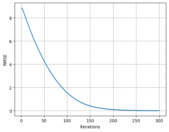
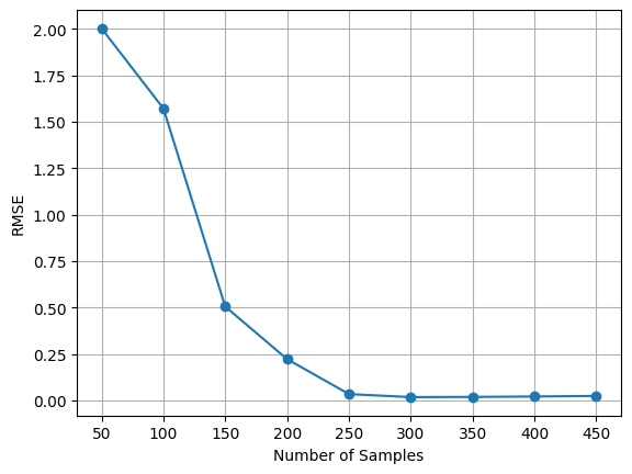
Figure 1. Plotted on the left is the average RMSE $F({\boldsymbol{\Theta}}_{n}),1\leq n\leq 300$, over 100 trials, where $M=4,L=5$ and $S=100$ and ${\boldsymbol{\Theta}_{n}},1\leq n\leq 300$, are the parameters in the $n$-th iteration of the SGDM. The average energy $S^{-1}\|{\bf y}\|_{2}^{2}$ of the output data over 100 trial is $21.8736$, while the uniform bound $\|{\bf y}\|_{\infty}=\sup_{1\leq i\leq S}|y_{i}|$ over 100 trial is $6.4467$. Presented on the right is the the average RMSE $F({\boldsymbol{\Theta}}_{\rm Iter})$ over 100 trials with respect to different sampling size $S$, where $M=4$, $L=5$ and ${\rm Iter}=100$.

Define the relative uniform approximation error (RUAE) of the GCNN with parameter ${\boldsymbol{\Theta}}$ by

$$U({\boldsymbol{\Theta}}):=\frac{\sup_{1\leq i\leq S}|f({\bf x}_{i})-f_{M}({\bf x}_{i},{\boldsymbol{\Theta}})|}{\sup_{1\leq i\leq S}|f({\bf x}_{i})|+10^{-6}},$$

where $f$ is the original function and $f_{M}({\bf x},{\boldsymbol{\Theta}})$ is the out of the GCNN given in (6.2). Presented in Figure 2 is how the RMSE and RUAE vary with the number of neurons per vertex. This demonstrates the theoretical result in Theorems 4.1 and 4.3 on the approximation property of GCNNs. We observe from Figure 2 that increasing the number of neurons at each vertex generally improves the accuracy of the GCNN, as measured by both RMSE and RUAE, as long as the number of iterations in SGDM is not too high. However, when the number of iterations is high (then RMSE and RUAE are low), adding more neurons does not help and may even hurt the performance of the GCNN. We hypothesize that this is because the GCNN becomes overfitted to the training data and loses its ability to generalize to new data.

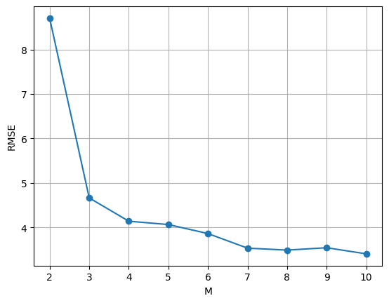
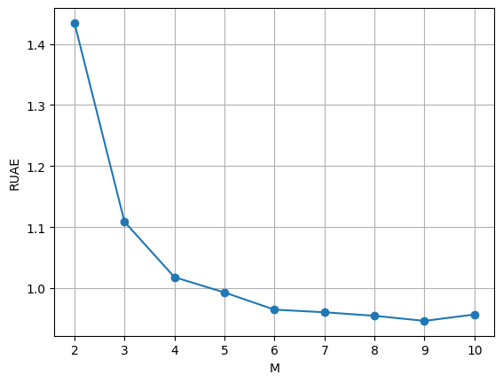
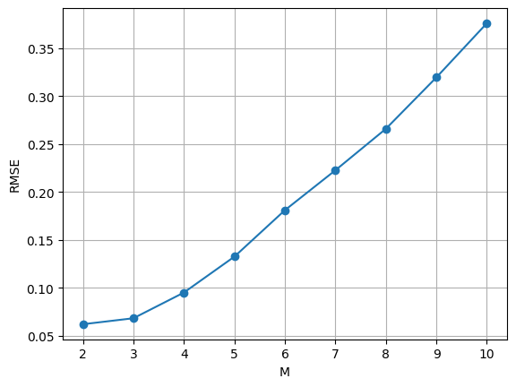
Figure 2. Plotted are the average RMSE $F({\boldsymbol{\Theta}}_{\rm Iter})$ (left) and RUAE $U({\boldsymbol{\Theta}}_{\rm Iter})$ (right) over 100 trials with respect to different number $M$ of neurons per vertex, where $S=100,L=5$, and ${\rm Iter}=50$ (top left and right) and $200$ (bottom left and right) respectively.

In the second simulation, we consider the real data set of hourly temperature measured in Celsius collected at $32$ weather stations in the region of Brest (France) in January 2014. Denote the regional temperature at $t_{i}$-th hour of $d$-th day by ${\bf x}^{\rm org}_{d}(t_{i}),0\leq i\leq 23,1\leq d\leq 31$. Before we apply GCNNs to learn functions, we pre-process the temperature data set by eliminating the average temperature and rescaling the range to $[-1,1]$,

$${\bf x}_{d}(t_{i})=B^{-1}\big{(}{\bf x}^{\rm org}_{d}(t_{i})-{\bf x}^{\rm org}_{\rm ave}\big{)},$$

where ${\bf x}^{\rm org}_{\rm ave}=(23\times 31)^{-1}\sum_{i=0}^{23}\sum_{d=1}^{31}{\bf x}_{d}^{\rm org}(t_{i})$ the average temperature in the region of Brest (France) for January 2014, and $B$ is chosen so that ${\bf x}_{d}(t_{i})\in[-1,1]$ for all $1\leq d\leq 31$ and $0\leq i\leq 23$. In particular, we take $B=10.35$ in our simulation. In the second simulation, we want to learn GCNNs to approximate the squared variance function $f_{\rm sv}$ of next day,

(6.7) $$f_{\rm sv}({\bf x}_{d}(t_{i}))=\|{\bf x}_{d+1}(t_{i})\|_{2}^{2}-({\bar{\bf x}}_{d+1}(t_{i}))^{2},\ 1\leq d\leq 30,0\leq i\leq 23,$$

where ${\bar{\bf x}}_{d+1}(t_{i})$ is the average pre-processed temperature data of the whole Brest region at $t_{i}$-th hour of $(d+1)$-th day.

Learning GCNNs from real-world data is a challenging task. In the second simulation, we try to learn GCNN from about 20% of the weather data set, particularly, ${\bf x}_{d}(t_{i})$ and $f_{\rm sv},0\leq i\leq 23,d\in\{1,6,11,16,21,26\}$, to learn the squared variance function $f_{\rm sv}$ of next day. Shown in Figure 3 is the approximation property of the output of the GCNN obtained from the SGDM, where the relative mean square error (RMSE) and relative uniform approximation error (RUAE) on the whole weather data set are defined by

$${\rm WMSE}=\frac{\sum_{i=0}^{23}\sum_{d=1}^{30}|f_{\rm sv}({\bf x}_{d}(t_{i}))-f_{M}({\bf x}_{d}(t_{i}),{\boldsymbol{\Theta}}_{\rm Iter})|^{2}}{\sum_{i=0}^{23}\sum_{d=1}^{30}|f_{\rm sv}({\bf x}_{d}(t_{i}))|^{2}}$$

and on the right is the uniform error

$${\rm WUAE}=\frac{\sup_{1\leq d\leq 30,0\leq i\leq 23}|f_{\rm sv}({\bf x}_{d}(t_{i}))-f_{M}({\bf x}_{d}(t_{i}),{\boldsymbol{\Theta}}_{\rm Iter})|}{\sup_{1\leq d\leq 30,0\leq i\leq 23}|f_{\rm sv}({\bf x}_{d}(t_{i})|},$$

where ${\boldsymbol{\Theta}}_{\rm Iter}$ is the output parameter of the SGDM. Comparing with the approximation of the quadratic function $f$ in (6.6) with the squared variance function $f_{\rm sv}$ in (6.7) by GCNNs, the number of neurons at each vertex has a positive impact on the accuracy of the GCNN, when the number of iterations in SGDM is not too high. However, when the number of iterations is high, adding more neurons does not improve and may even degrade the performance of the GCNN.

From the approximation property presented by Figures 2 and 3, we observe that there is a trade-off between the number $M$ of neurons and the number ${\rm Iter}$ of iterations in the SGDM that needs to be carefully balanced to achieve the optimal performance of the GCNNs.

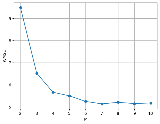
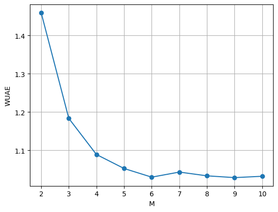
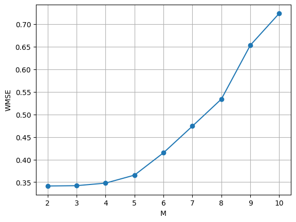
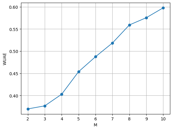
Figure 3. Plotted are the average WMSE (left) and WUAE (right) over 100 trials with respect to different number $M$ of neurons per vertex, where $S=218=24\times 12,L=5$, and ${\rm Iter}=30$ (top left and right) and $100$ (bottom left and right) respectively.

7. Proofs

In this section, we collect the proofs of Theorems 3.1, 3.3, 3.6, 4.1, 4.3, 4.4, 4.5, 5.1 and 5.2.

7.1. Proof of Theorem 3.1

To prove Theorem 3.1, we first show that $\|\cdot\|_{{\mathcal{B}}_{1}}$ in (3.3) defines a norm on the Barron space ${\mathcal{B}}_{1}$.

Lemma 7.1.

Let $\|\cdot\|_{{\mathcal{B}}_{1}}$ be as in (3.3). Then

• $f=0$ if and only if $\|f\|_{{\mathcal{B}}_{1}}=0$.

• $\|\alpha f\|_{{\mathcal{B}}_{1}}=|\alpha|\|f\|_{{\mathcal{B}}_{1}}$ for all $f\in{\mathcal{B}}_{1}$ and $\alpha\in{\mathbb{R}}$.

• $\|f+g\|_{{\mathcal{B}}_{1}}\leq\|f\|_{{\mathcal{B}}_{1}}+\|g\|_{{\mathcal{B}}_{1}}$ for all $f,g\in{\mathcal{B}}_{1}$.

Proof.

(i)  Taking the Dirac measure $\delta_{0}$ at the origin as the probability measure in (3.2) gives a representation for the zero function. This shows that $\|f\|_{{\mathcal{B}}_{1}}=0$ for the zero function $f=0$. Conversely, given $f\in{\mathcal{B}}_{1}$ with $\|f\|_{{\mathcal{B}}_{1}}=0$, there exists a probability measure $\rho$ for any $\epsilon>0$ such that (3.2) holds and ${\mathbb{E}}_{\rho}(\|{\bf a}\|_{*}(\|{\bf b}\|_{\rm co}+\|{\bf c}\|))\leq\epsilon$. Therefore for any ${\bf x}\in\Omega$, we have

$$|f({\bf x})| \hskip-5.78172pt\leq \hskip-5.78172pt\int_{{\mathbb{R}}^{N}\times{\mathcal{W}}\times{\mathbb{R}}^{N}}\|{\bf a}\|_{*}(\|{\bf b}\|_{\rm co}+\|{\bf c}\|)\rho(d{\bf a},d{\bf b},d{\bf c})$$

$$\hskip-5.78172pt= \hskip-5.78172pt{\mathbb{E}}_{\rho}(\|{\bf a}\|_{*}(\|{\bf b}\|_{\rm co}+\|{\bf c}\|))\leq\epsilon.$$

As $\epsilon>0$ is arbitrary chosen, we conclude that $f$ must be the zero function. This proves the conclusion (i).

(ii)  Clearly it suffices to show that

(7.1) $$\|\alpha f\|_{{\mathcal{B}}_{1}}\leq|\alpha|\|f\|_{{\mathcal{B}}_{1}}$$

for all $0\neq\alpha\in{\mathbb{R}}$ and $f\in{\mathcal{B}}_{1}$. Take arbitrary $\epsilon>0$ and let $\rho$ be a probability measure in ${\mathcal{P}}_{f}$ such that

(7.2) $${\mathbb{E}}_{\rho}(\|{\bf a}\|_{*}(\|{\bf b}\|_{\rm co}+\|{\bf c}\|))\leq\|f\|_{{\mathcal{B}}_{1}}+\epsilon.$$

Define a new probability measure $\tilde{\rho}(A)=\rho(\tilde{A})$ for any Borel set $A$, where $\tilde{A}=\{({\bf a},{\bf b},{\bf c})|({\bf a}/\alpha,{\bf b},{\bf c})\in A\}$. Then one may verify that

$$\alpha f({\bf x}) \hskip-5.78172pt= \hskip-5.78172pt\int_{({\bf a},{\bf b},{\bf c})\in{\mathbb{R}}^{N}\times{\mathcal{W}}\times{\mathbb{R}}^{N}}(\alpha{\bf a})^{T}\sigma({\bf b}*{\bf x}+{\bf c})\rho(d{\bf a},d{\bf b},d{\bf c})$$

$$\hskip-5.78172pt= \hskip-5.78172pt\int_{(\tilde{\bf a},{\bf b},{\bf c})\in{\mathbb{R}}^{N}\times{\mathcal{W}}\times{\mathbb{R}}^{N}}\tilde{\bf a}^{T}\sigma({\bf b}*{\bf x}+{\bf c})\tilde{\rho}(d\tilde{\bf a},d{\bf b},d{\bf c})$$

and

$${\mathbb{E}}_{\tilde{\rho}}\big{(}\|{\bf a}\|_{*}(\|{\bf b}\|_{\rm co}+\|{\bf c}\|)\big{)} \hskip-5.78172pt= \hskip-5.78172pt\int_{({\bf a},{\bf b},{\bf c})\in{\mathbb{R}}^{N}\times{\mathcal{W}}\times{\mathbb{R}}^{N}}\|{\bf a}\|_{*}(\|{\bf b}\|_{\rm co}+\|{\bf c}\|)\tilde{\rho}(d{\bf a},d{\bf b},d{\bf c})$$

$$\hskip-5.78172pt= \hskip-5.78172pt\int\|\alpha\tilde{\bf a}\|_{*}(\|{\bf b}\|_{\rm co}+\|{\bf c}\|)\rho(d\tilde{\bf a},d{\bf b},d{\bf c})$$

$$\hskip-5.78172pt= \hskip-5.78172pt|\alpha|{\mathbb{E}}_{\tilde{\rho}}(\|\tilde{\bf a}\|_{*}(\|{\bf b}\|_{\rm co}+\|{\bf c}\|))\leq|\alpha|\|f\|_{{\mathcal{B}}_{1}}+|\alpha|\epsilon.$$

Then the desired estimate (7.1) follows from the above estimate and the arbitrary selection of $\epsilon>0$.

(iii)    By the second conclusion, it suffices to prove that

(7.3) $$\|\alpha f_{1}+(1-\alpha)f_{2}\|_{{\mathcal{B}}_{1}}\leq\alpha\|f_{1}\|_{{\mathcal{B}}_{1}}+(1-\alpha)\|f_{2}\|_{{\mathcal{B}}_{1}},\ f_{1},f_{2}\in{\mathcal{B}}_{1}$$

where $0\leq\alpha\leq 1$. Take arbitrary $\epsilon>0$ and let $\rho_{1}\in{\mathcal{P}}_{f_{1}}$ and $\rho_{2}\in{\mathcal{P}}_{f_{2}}$ be two probability measures so that

(7.4) $${\mathbb{E}}_{\rho_{l}}(\|{\bf a}\|_{*}(\|{\bf b}\|_{\rm co}+\|{\bf c}\|))\leq\|f_{l}\|_{{\mathcal{B}}_{1}}+\epsilon,\ l=1,2.$$

Define $\rho=\alpha\rho_{1}+(1-\alpha)\rho_{2}$ and set $f=\alpha f_{1}+(1-\alpha)f_{2}$. Then one may verify that $\rho$ is a probability measure in ${\mathcal{P}}_{f}$ and

$${\mathbb{E}}_{\rho}(\|{\bf a}\|_{*}(\|{\bf b}\|_{\rm co}+\|{\bf c}\|))\leq\alpha\|f_{1}\|_{{\mathcal{B}}_{1}}+(1-\alpha)\|f_{2}\|_{{\mathcal{B}}_{1}}+\epsilon.$$

This together with the arbitrary selection of $\epsilon>0$ proves (7.3). ∎

To prove Theorem 3.1, we next show that the probability measure $\rho$ in the representation (3.2) of any function $f$ in ${\mathcal{B}}_{1}$ could be selected to be supported on the dilated unit sphere.

Lemma 7.2.

Let ${\mathbb{S}}$ and ${\mathbb{T}}$ be as in (3.7). Then for any $f\in{\mathcal{B}}_{1}$, there exists a probability measure $\hat{\rho}$ supported on ${\mathbb{S}}\times{\mathbb{T}}$ such that

(7.5) $$f({\bf x})=\|f\|_{{\mathcal{B}}_{1}}\int_{{\mathbb{S}}\times{\mathbb{T}}}{\bf a}^{T}\sigma({\bf b}*{\bf x}+{\bf c})\hat{\rho}(d{\bf a},d{\bf b},d{\bf c}),\ {\bf x}\in\Omega.$$

Proof.

The conclusion is obvious for the zero function. Now we assume that $f\neq 0$. By (3.3), there exist probability measures $\rho_{n}\in{\mathcal{P}}_{f},n\geq 1$, on ${\mathbb{R}}^{N}\times{\mathcal{W}}\times{\mathbb{R}}^{N}$ such that

(7.6) $$\|f\|_{{\mathcal{B}}_{1}}\leq A_{n}:={\mathbb{E}}_{\rho_{n}}\big{(}\|{\bf a}\|_{*}(\|{\bf b}\|_{\rm co}+\|{\bf c}\|)\big{)}\leq\|f\|_{{\mathcal{B}}_{1}}+2^{-n},\ n\geq 1.$$

For $n\geq 1$, define the measure $\hat{\rho}_{n}(E)$ of a Borel measurable subset $E\subset{\mathbb{S}}\times{\mathbb{T}}$ by

$$\hat{\rho}_{n}(E)=A_{n}^{-1}{\mathbb{E}}_{\rho_{n}}\big{(}\|{\bf a}\|_{*}(\|{\bf b}\|_{{\rm co}}+\|{\bf c}\|)\chi_{\hat{E}}({\bf a},{\bf b},{\bf c})\big{)}$$

where

$${\hat{E}}=\Big{\{}({\bf a},{\bf b},{\bf c})\in{\mathbb{R}}^{N}\times{\mathcal{W}}\times{\mathbb{R}}^{N}:\ \Big{(}\frac{{\bf a}}{\|{\bf a}\|_{*}},\frac{{\bf b}}{\|{\bf b}\|_{\rm co}+\|{\bf c}\|},\frac{{\bf c}}{\|{\bf b}\|_{\rm co}+\|{\bf c}\|}\Big{)}\in E\Big{\}},$$

and $\chi_{\hat{E}}$ is the characteristic function on the set $\hat{E}$. One may verify that $\hat{\rho}_{n},n\geq 1$, are probability measures on ${\mathbb{S}}\times{\mathbb{T}}$, and

(7.7) $$f({\bf x}) = \int_{{\mathbb{R}}^{N}\times{\mathcal{W}}\times{\mathbb{R}}^{N}}{\bf a}^{T}\sigma({\bf b}*{\bf x}+{\bf c})\rho_{n}(d{\bf a},d{\bf b},d{\bf c})$$

$$= \int_{{\mathbb{R}}^{N}\times{\mathcal{W}}\times{\mathbb{R}}^{N}}\|{\bf a}\|_{*}(\|{\bf b}\|_{\rm co}+\|{\bf c}\|)$$

$$\times\Big{(}\frac{{\bf a}}{\|{\bf a}\|_{*}}\Big{)}^{T}\sigma\Big{(}\frac{\bf b}{\|{\bf b}\|_{\rm co}+\|{\bf c}\|}*{\bf x}+\frac{{\bf c}}{\|{\bf b}\|_{\rm co}+\|{\bf c}\|}\Big{)}\rho_{n}(d{\bf a},d{\bf b},d{\bf c})$$

$$= A_{n}\int_{{\mathbb{S}}\times{\mathbb{T}}}{\hat{\bf a}}^{T}\sigma\big{(}\hat{\bf b}*{\bf x}+\hat{\bf c})\hat{\rho}_{n}(d\hat{\bf a},d\hat{\bf b},d\hat{\bf c}).$$

Recall that $\hat{\rho}_{n},n\geq 1$, is a sequence of probability measures on the compact set ${\mathbb{S}}\times{\mathbb{T}}$. Then by Prokhorov theorem [43], without loss of generality, we assume that $\hat{\rho}_{n},n\geq 1$, converges weakly to a probability measure $\hat{\rho}$ on ${\mathbb{S}}\times{\mathbb{T}}$

(7.8) $$\lim_{n\to\infty}\hat{\rho}_{n}=\hat{\rho}\ \ {\rm weakly},$$

otherwise replacing the sequence by a weakly convergent subsequence. For any ${\bf x}\in\Omega$, the function ${\bf a}^{T}({\bf b}*{\bf x}+{\bf c})$ is continuous with respect to $({\bf a},{\bf b},{\bf c})\in{\mathbb{S}}\times{\mathbb{T}}$ and is bounded by one. Therefore the desired conclusion (7.5) follows from (7.6), (7.7) and (7.8). ∎

Now we are ready to prove Theorem 3.1.

Proof of Theorem 3.1.

First we prove that ${\mathcal{B}}_{1}$ is a Banach space. By Lemma 7.1, it suffices to prove every Cauchy sequence $f_{n},n\geq 1$, in ${\mathcal{B}}_{1}$ converges to some function in ${\mathcal{B}}_{1}$. In particular, without loss of generality, we may assume that

(7.9) $$\|f_{n+1}-f_{n}\|_{{\mathcal{B}}_{1}}\leq 2^{-n},\ n\geq 1,$$

other replacing it by one of its subsequences satisfying (7.9).

By Lemma 7.2, there exist probability measures $\hat{\rho}_{n},n\geq 1$, on ${\mathbb{S}}\times{\mathbb{T}}$ such that

(7.10) $$f_{1}({\bf x})=\|f_{1}\|_{{\mathcal{B}}_{1}}\int_{{\mathbb{S}}\times{\mathbb{T}}}{\bf a}^{T}\sigma({\bf b}*{\bf x}+{\bf c})\hat{\rho}_{1}(d{\bf a},d{\bf b},d{\bf c})$$

and

(7.11) $$f_{n}({\bf x})-f_{n-1}({\bf x})=\|f_{n}-f_{n-1}\|_{{\mathcal{B}}_{1}}\int_{{\mathbb{S}}\times{\mathbb{T}}}{\bf a}^{T}\sigma({\bf b}*{\bf x}+{\bf c})\hat{\rho}_{n}(d{\bf a},d{\bf b},d{\bf c}),\ {\bf x}\in\Omega$$

for all $n\geq 2$. Define

(7.12) $$f({\bf x})=A\int_{{\mathbb{S}}\times{\mathbb{T}}}{\bf a}^{T}\sigma({\bf b}*{\bf x}+{\bf c})\hat{\rho}(d{\bf a},d{\bf b},d{\bf c}),\ {\bf x}\in\Omega,$$

where $A=\|f_{1}\|_{{\mathcal{B}}_{1}}+\sum_{n=2}^{\infty}\|f_{n}-f_{n-1}\|_{{\mathcal{B}}_{1}}<\infty$ and the probability measure $\hat{\rho}$ on ${\mathbb{S}}\times{\mathbb{T}}$ is given by

(7.13) $$\hat{\rho}=A^{-1}\Big{(}\|f_{1}\|_{{\mathcal{B}}_{1}}\hat{\rho}_{1}+\sum_{n=2}^{\infty}\|f_{n}-f_{n-1}\|_{{\mathcal{B}}_{1}}\hat{\rho}_{n}\Big{)}.$$

Dilate the measure $\hat{\rho}$ on ${\mathbb{S}}\times{\mathbb{T}}$ to a probability measure on $(A{\mathbb{S}})\times{\mathbb{T}}$ and then extend to a probability measure on ${\mathbb{R}}^{N}\times{\mathcal{W}}\times{\mathbb{R}}^{N}$ with support on $(A{\mathbb{S}})\times{\mathbb{T}}$. Denote the dilated extension measure by $\tilde{\rho}$. By (7.12) and (7.13), the dilated extension measure $\tilde{\rho}$ is a probability measure on ${\mathbb{R}}^{N}\times{\mathcal{W}}\times{\mathbb{R}}^{N}$ satisfying (3.2), i.e., $\tilde{\rho}\in{\mathcal{P}}_{f}$. Again from (7.12) and (7.13) we obtain

$$\|f\|_{{\mathcal{B}}_{1}}\leq{\mathbb{E}}_{\tilde{\rho}}(\|{\bf a}\|_{*}(\|{\bf b}\|_{\rm co}+\|{\bf c}\|))=A,$$

which proves that $f\in{\mathcal{B}}_{1}$.

Dilate and extend the probability measure $\hat{\rho}_{m},m\geq 1$ on ${\mathbb{S}}\times{\mathbb{T}}$ to probability measures $\tilde{\rho}_{m}$ on ${\mathbb{R}}^{N}\times{\mathcal{W}}\times{\mathbb{R}}^{N}$ with support on ${\mathbb{S}}\times{\mathbb{T}}$. We observe that

$$\|f_{n}-f\|_{{\mathcal{B}}_{1}} \hskip-5.78172pt= \hskip-5.78172pt\Big{\|}\sum_{m=n+1}^{\infty}\|f_{m}-f_{m-1}\|_{{\mathcal{B}}_{1}}\int_{{\mathbb{S}}\times{\mathbb{T}}}{\bf a}^{T}\sigma({\bf b}*{\bf x}+{\bf c})\hat{\rho}_{m}(d{\bf a},d{\bf b},d{\bf c})\Big{\|}_{{\mathcal{B}}_{1}}$$

$$\hskip-5.78172pt\leq \hskip-5.78172pt\sum_{m=n+1}^{\infty}\|f_{m}-f_{m-1}\|_{{\mathcal{B}}_{1}}\Big{\|}\int_{{\mathbb{S}}\times{\mathbb{T}}}{\bf a}^{T}\sigma({\bf b}*{\bf x}+{\bf c})\hat{\rho}_{m}(d{\bf a},d{\bf b},d{\bf c})\Big{\|}_{{\mathcal{B}}_{1}}$$

$$\hskip-5.78172pt\leq \hskip-5.78172pt\sum_{m=n+1}^{\infty}\|f_{m}-f_{m-1}\|_{{\mathcal{B}}_{1}}{\mathbb{E}}_{\tilde{\rho}_{m}}(\|{\bf a}\|_{*}(\|{\bf b}\|_{\rm co}+\|{\bf c}\|))\leq 2^{-n+1},$$

where the equality holds by (7.10), (7.11) and (7.12), and the first, second and third inequality follows from Lemma 7.1, the definition of Barron norm and (7.9) respectively. Therefore $f_{n},n\geq 1$, converges to $f\in{\mathcal{B}}_{1}$ and hence ${\mathcal{B}}_{1}$ is a Banach space.

By (2.17), (2.19) and (7.5), we have

$$|f({\bf x})| \hskip-5.78172pt\leq \hskip-5.78172pt\|f\|_{{\mathcal{B}}_{1}}\int_{{\mathbb{S}}\times{\mathbb{T}}}|{\bf a}^{T}\sigma({\bf b}*{\bf x}+{\bf c})|\hat{\rho}(d{\bf a},d{\bf b},d{\bf c})$$

$$\hskip-5.78172pt\leq \hskip-5.78172pt\|f\|_{{\mathcal{B}}_{1}}\int_{{\mathbb{S}}\times{\mathbb{T}}}\|{\bf a}\|_{*}\|{\bf b}*{\bf x}+{\bf c}\|\hat{\rho}(d{\bf a},d{\bf b},d{\bf c})$$

$$\hskip-5.78172pt\leq \hskip-5.78172pt\|f\|_{{\mathcal{B}}_{1}}\int_{{\mathbb{S}}\times{\mathbb{T}}}\|{\bf a}\|_{*}(\|{\bf b}\|_{\rm co}+\|{\bf c}\|)\hat{\rho}(d{\bf a},d{\bf b},d{\bf c})=\|f\|_{{\mathcal{B}}_{1}}.$$

This proves the reproducing kernel property (3.4) for the Banach space ${\mathcal{B}}_{1}$.

Applying Hölder inequality, we have

(7.14) $$\|f\|_{{\mathcal{B}}_{1}}\leq\|f\|_{{\mathcal{B}}_{r}}\leq\|f\|_{{\mathcal{B}}_{\infty}}\ {\rm for\ all}\ f\in{\mathcal{B}}_{\infty}\ {\rm and}\ 1\leq r\leq\infty.$$

Therefore the proof of the norm equivalence in (3.5) reduces to establishing

(7.15) $$\|f\|_{{\mathcal{B}}_{\infty}}\leq\|f\|_{{\mathcal{B}}_{1}}\ {\rm for\ all}\ f\in{\mathcal{B}}_{1}.$$

By Lemma 7.2, there exist a probability measure $\hat{\rho}$ on ${\mathbb{S}}\times{\mathbb{T}}$ such that

(7.16) $$f({\bf x})=\|f\|_{{\mathcal{B}}_{1}}\int_{{\mathbb{S}}\times{\mathbb{T}}}{\bf a}^{T}\sigma({\bf b}*{\bf x}+{\bf c})\hat{\rho}(d{\bf a},d{\bf b},d{\bf c}).$$

Dilate the measure $\hat{\rho}$ on ${\mathbb{S}}\times{\mathbb{T}}$ to a probability measure on $(\|f\|_{{\mathcal{B}}_{1}}{\mathbb{S}})\times{\mathbb{T}}$ and then extend to a probability measure $\tilde{\rho}$ on ${\mathbb{R}}^{N}\times{\mathcal{W}}\times{\mathbb{R}}^{N}$ with support on $(\|f\|_{{\mathcal{B}}_{1}}{\mathbb{S}})\times{\mathbb{T}}$. Then one may verify that $\tilde{\rho}\in{\mathcal{P}}_{f}$ and

$$\|f\|_{{\mathcal{B}}_{\infty}}\leq\sup_{({\bf a},{\bf b},{\bf c})\in{\rm supp}\tilde{\rho}}\|{\bf a}\|_{*}(\|{\bf b}\|_{\rm co}+\|{\bf c}\|)=\|f\|_{{\mathcal{B}}_{1}}.$$

This proves (7.15). Hence the desired conclusion that ${\mathcal{B}}_{r},1\leq r\leq\infty$, are Banach spaces independent on $1\leq r\leq\infty$. ∎

7.2. Proof of Theorem 3.3

Let ${\mathcal{L}}_{\hat{\rho}}^{o}$ be the linear space spanned by ${\bf a}^{T}\sigma({\bf b}*{\bf x}+{\bf c}),{\bf x}\in\Omega$. One may verify that $g\in{\mathcal{H}}^{o}_{\hat{\rho}}$ if and only if $g=\sum_{i=1}^{I}c_{i}K_{\hat{\rho}}(\cdot,{\bf x}_{i})$ for some $c_{i}\in{\mathbb{R}}$ and ${\bf x}_{i}\in\Omega,1\leq i\leq I$, if and only if

(7.17) $$g({\bf x})=\int_{{\mathbb{S}}\times{\mathbb{T}}}{\bf a}^{T}\sigma({\bf b}*{\bf x}+{\bf c})\eta({\bf a},{\bf b},{\bf c})\hat{\rho}(d{\bf a},d{\bf b},d{\bf c})$$

for some function $\eta\in{\mathcal{L}}_{\hat{\rho}}^{o}$. Moreover,

(7.18) $$\|g\|_{{\mathcal{H}}_{\hat{\rho}}}=\Big{(}\int_{{\mathbb{S}}\times{\mathbb{T}}}|\eta({\bf a},{\bf b},{\bf c})|^{2}\hat{\rho}(d{\bf a},d{\bf b},d{\bf c})\Big{)}^{1/2}$$

and

(7.19) $$|g({\bf x})| \hskip-5.78172pt\leq \hskip-5.78172pt\int_{{\mathbb{S}}\times{\mathbb{T}}}|{\bf a}^{T}\sigma({\bf b}*{\bf x}+{\bf c})||\eta({\bf a},{\bf b},{\bf c})|\hat{\rho}(d{\bf a},d{\bf b},d{\bf c})$$

$$\hskip-5.78172pt\leq \hskip-5.78172pt\int_{{\mathbb{S}}\times{\mathbb{T}}}|\eta({\bf a},{\bf b},{\bf c})|\hat{\rho}(d{\bf a},d{\bf b},d{\bf c})$$

$$\hskip-5.78172pt\leq \hskip-5.78172pt\Big{(}\int_{{\mathbb{S}}\times{\mathbb{T}}}|\eta({\bf a},{\bf b},{\bf c})|^{2}\hat{\rho}(d{\bf a},d{\bf b},d{\bf c})\Big{)}^{1/2}=\|g\|_{{\mathcal{H}}_{\hat{\rho}}},\ {\bf x}\in\Omega.$$

This proves (3.11), (3.12) and (3.13) for functions $g\in{\mathcal{H}}_{\hat{\rho}}^{o}$. Recall that ${\mathcal{H}}_{\hat{\rho}}$ and ${\mathcal{L}}_{\hat{\rho}}^{2}$ are the completion of ${\mathcal{H}}_{\hat{\rho}}^{o}$ and ${\mathcal{L}}_{\hat{\rho}}^{o}$ respectively. Hence taking limits in (7.17), (7.18) and (7.19), and using the reproducing kernel property of ${\mathcal{H}}_{\hat{\rho}}$ and the conclusion in Remark 3.4 completes the proof.

7.3. Proof of Theorem 3.6

Take $f\in{\mathcal{B}}$ and let $\hat{\rho}\in\hat{P}$ be the probability measure on ${\mathbb{S}}\times{\mathbb{T}}$ such that (3.8) holds. Then by Theorem 3.3, we conclude that $f\in{\mathcal{H}}_{\hat{\rho}}$ and

$$\|f\|_{{\mathcal{H}}_{\hat{\rho}}}\leq\|f\|_{\mathcal{B}}\Big{(}\int_{{\mathbb{S}}\times{\mathbb{T}}}|(P_{\hat{\rho}}1)({\bf a},{\bf b},{\bf c})|^{2}\hat{\rho}(d{\bf a},d{\bf b},d{\bf c})\Big{)}^{1/2}\leq\|f\|_{\mathcal{B}}.$$

This shows that

(7.20) $${\mathcal{B}}\subset\cup_{{\hat{\rho}}\in\widehat{P}}{\mathcal{H}}_{\hat{\rho}}\ \ {\rm and}\ \ \inf_{f\in H_{\hat{\rho}},\hat{\rho}\in\hat{P}}\|f\|_{{\mathcal{H}}_{\hat{\rho}}}\leq\|f\|_{\mathcal{B}}.$$

Let $f\in{\mathcal{H}}_{\hat{\rho}}$ for some $\hat{\rho}\in\hat{P}$ and $\eta\in{\mathcal{L}}_{\hat{\rho}}^{2}$ so that (3.11) holds. The existence of such a function $\eta$ follows from (3.14) and Theorem 3.3. Moreover, we have

(7.21) $$\|f\|_{{\mathcal{H}}_{\hat{\rho}}}=\|\eta\|_{L^{2}_{\hat{\rho}}}.$$

Define a probability measure $\hat{\tilde{\rho}}$ on ${\mathbb{S}}\times{\mathbb{T}}$ by

(7.22) $$\hat{\tilde{\rho}}(A)=\frac{\int_{E_{1}\cap A}\eta({\bf a},{\bf b},{\bf c})\hat{\rho}(d{\bf a},d{\bf b},d{\bf c})-\int_{E_{2}\cap\tilde{A}}\eta({\bf a},{\bf b},{\bf c})\hat{\rho}(d{\bf a},d{\bf b},d{\bf c})}{\|\eta\|_{L^{1}_{\hat{\rho}}}},$$

where $E_{1}=\{({\bf a},{\bf b},{\bf c})\in{\mathbb{S}}\times{\mathbb{T}}:\ \eta({\bf a},{\bf b},{\bf c})\geq 0\}$, $E_{2}=\{({\bf a},{\bf b},{\bf c})\in{\mathbb{S}}\times{\mathbb{T}}:\ \eta({\bf a},{\bf b},{\bf c})<0\}$, and $\tilde{A}=\{({\bf a},{\bf b},{\bf c})\in{\mathbb{S}}\times{\mathbb{T}}:\ (-{\bf a},{\bf b},{\bf c})\in A\}$. By (3.11) and the definition (7.22) of the probability measure $\hat{\tilde{\rho}}\in\hat{P}$, we have

$$f({\bf x}) \hskip-5.78172pt= \hskip-5.78172pt\int_{E_{1}}{\bf a}^{T}\sigma({\bf b}*{\bf x}+{\bf c})\eta({\bf a},{\bf b},{\bf c})\hat{\rho}(d{\bf a},d{\bf b},d{\bf c})$$

$$\hskip-5.78172pt+\int_{E_{2}}(-{\bf a})^{T}\sigma({\bf b}*{\bf x}+{\bf c})(-\eta)({\bf a},{\bf b},{\bf c})\hat{\rho}(d{\bf a},d{\bf b},d{\bf c})$$

$$\hskip-5.78172pt= \hskip-5.78172pt\|\eta\|_{L^{1}_{\hat{\rho}}}\int_{{\mathbb{S}}\times{\mathbb{T}}}{\bf a}^{T}\sigma({\bf b}*{\bf x}+{\bf c})\eta({\bf a},{\bf b},{\bf c})\hat{\tilde{\rho}}(d{\bf a},d{\bf b},d{\bf c}).$$

This implies that $f\in{\mathcal{B}}$ and $\|f\|_{\mathcal{B}}\leq\|\eta\|_{L^{1}_{\hat{\rho}}}$. This together with (7.21) and the observation $\|\eta\|_{L^{1}_{\hat{\rho}}}\leq\|\eta\|_{L^{2}_{\hat{\rho}}}$ implies that

(7.23) $${\mathcal{H}}_{\hat{\rho}}\subset{\mathcal{B}}\ \ {\rm and}\ \ \|f\|_{\mathcal{B}}\leq\|f\|_{{\mathcal{H}}_{\hat{\rho}}}\ {\rm for\ all}\ f\in{\mathcal{H}}_{\hat{\rho}}.$$

Combining (7.21) and (7.23) completes the proof.

7.4. Proof of Theorem 4.1

Without loss of generality, we assume that $f\in{\mathcal{B}}$ is a nonzero function with $\|f\|_{\mathcal{B}}=1$, otherwise replacing $f$ by $f/\|f\|_{\mathcal{B}}$. Then by Lemma 7.2, there exists a probability measure $\hat{\rho}$ on ${\mathbb{S}}\times{\mathbb{T}}$ such that

(7.24) $$f({\bf x})=\int_{{\mathbb{S}}\times{\mathbb{T}}}{\bf a}^{T}\sigma({\bf b}*{\bf x}+{\bf c})\hat{\rho}(d{\bf a},d{\bf b},d{\bf c}),\ {\bf x}\in\Omega.$$

Let ${\boldsymbol{\theta}}_{m}=({\bf a}_{m},{\bf b}_{m},{\bf c}_{m})\in{\mathbb{S}}\times{\mathbb{T}},1\leq m\leq M$, be i.i.d. random variables following the probability measure $\hat{\rho}$. Set ${\boldsymbol{\Theta}}=({\boldsymbol{\theta}}_{1},\ldots,{\boldsymbol{\theta}}_{M})$ and define

$$f_{M}({\bf x},{\boldsymbol{\Theta}})=\frac{1}{M}\sum_{m=1}^{M}\phi({\bf x},\theta_{m}),\ \ {\bf x}\in\Omega.$$

Clearly, we have

$$\|{\boldsymbol{\Theta}}\|_{P,\infty}=1=\|f\|_{\mathcal{B}}.$$

Observe that $\phi({\bf x},\boldsymbol{\theta}_{m})={\bf a}_{m}^{T}\sigma({\bf b}_{m}*{\bf x}+{\bf c}_{m})$ are i.i.d random variables with $\phi({\bf x},\boldsymbol{\theta}_{m})\in[-1,1]$ almost surely and ${\mathbb{E}}\phi({\bf x},\boldsymbol{\theta}_{m})=f({\bf x})$ hold for all $1\leq m\leq M$ and ${\bf x}\in\Omega$. Combining the above observation with (1.1) and (7.24), we obtain

$${\mathbb{E}}\int_{\Omega}(f_{M}({\bf x},{\boldsymbol{\Theta}})-f({\bf x}))^{2}d\mu({\bf x}) \hskip-5.78172pt= \hskip-5.78172pt\frac{1}{M}\int_{\Omega}{\mathbb{E}}(\phi({\bf x},\boldsymbol{\theta})-{\mathbb{E}}\phi({\bf x},\boldsymbol{\theta}))^{2}d\mu({\bf x})$$

$$\hskip-5.78172pt\leq \hskip-5.78172pt\frac{1}{M}\int_{\Omega}{\mathbb{E}}(\phi({\bf x},\boldsymbol{\theta}))^{2}d\mu({\bf x})\leq\frac{1}{M}.$$

Applying the Markov’s inequality yields

$${\mathbb{P}}\Big{\{}\int_{\Omega}(f_{M}({\bf x},{\boldsymbol{\Theta}})-f({\bf x}))^{2}d\mu({\bf x})>\frac{1+\epsilon}{M}\Big{\}}\leq\frac{1}{1+\epsilon}<1.$$

This completes the proof.

7.5. Proof of Theorem 4.3

We follow the argument of Theorem 4.1. Without loss of generality, we assume that $\|f\|_{\mathcal{B}}=1$. Let $\hat{\rho}$ be the probability measure on ${\mathbb{S}}\times{\mathbb{T}}$ in (7.24), ${\boldsymbol{\Theta}}=({\boldsymbol{\theta}}_{1},\ldots,{\boldsymbol{\theta}}_{M})$ be the i.i.d random variables following the probability measure $\hat{\rho}$, and define $f_{M}({\bf x},{\boldsymbol{\Theta}})$ be as in (1.1).

Set $I=N_{\epsilon}^{\rm ext}$ and take a family of balls $B({\bf x}_{i},\epsilon),1\leq i\leq I$, with center ${\bf x}_{i}\in\Omega$ and radius $\epsilon$ that covers the domain $\Omega$,

(7.25) $$\cup_{i=1}^{I}B({\bf x}_{i},\epsilon)=\Omega.$$

For any random variable ${\boldsymbol{\theta}}=({\bf a},{\bf b},{\bf c})\in{\mathbb{S}}\times{\mathbb{T}}$, we obtain from (1.1) and the definition of ${\mathbb{S}}\times{\mathbb{T}}$ that $\phi({\bf x}_{i},{\boldsymbol{\theta}})={\bf a}^{T}\sigma({\bf b}*{\bf x}_{i}+{\bf c})\in[-1,1]$ almost surely and ${\mathbb{E}}\phi({\bf x}_{i},{\boldsymbol{\theta}})=f({\bf x}_{i})$. Therefore $\phi({\bf x}_{i},\theta)-f({\bf x}_{i})$ is subGaussian with variance proxy 1 by Hoeffding’s inequality, i.e.,

$${\mathbb{E}}\exp\big{(}s(\phi({\bf x}_{i},{\boldsymbol{\theta}})-f({\bf x}_{i}))\big{)}\leq\exp(s^{2}/2),\ s\in{\mathbb{R}}.$$

Therefore for all $t>0$, we have

(7.26) $${\mathbb{P}}\{|f_{M}({\bf x}_{i},{\boldsymbol{\Theta}})-f({\bf x}_{i})|>t\}\leq 2\exp(-Mt^{2}/2).$$

This together with (4.10) implies the existence of ${\boldsymbol{\Theta}}^{*}\in({\mathbb{S}}\times{\mathbb{T}})^{M}$ such that

(7.27) $$\|{\boldsymbol{\Theta}}^{*}\|_{P,\infty}\leq 1=\|f\|_{\mathcal{B}}$$

and

(7.28) $$|f_{M}({\bf x}_{i},{\boldsymbol{\Theta}}^{*})-f({\bf x}_{i})|\leq\epsilon,\ 1\leq i\leq I.$$

For the above shallow GCNN with parameter ${\boldsymbol{\Theta}}^{*}$, we obtain from (4.2), (7.25), (7.28), and Corollary 3.2 that

$$|f_{M}({\bf x},{\boldsymbol{\Theta}}^{*})-f({\bf x})|$$

$$\hskip-5.78172pt\leq \hskip-5.78172pt|f_{M}({\bf x},{\boldsymbol{\Theta}}^{*})-f_{M}({\bf x}_{i},{\boldsymbol{\Theta}}^{*})|+|f_{M}({\bf x}_{i},{\boldsymbol{\Theta}}^{*})-f({\bf x}_{i})|+|f({\bf x})-f({\bf x}_{i})|$$

$$\hskip-5.78172pt\leq \hskip-5.78172ptD_{1}\|\sigma\|_{\rm Lip}\epsilon\|{\boldsymbol{\Theta}}^{*}\|_{P,\infty}+\epsilon+D_{1}\|\sigma\|_{\rm Lip}\epsilon\|f\|_{\mathcal{B}}\leq(2D_{1}\|\sigma\|_{\rm Lip}+1)\epsilon,\ {\bf x}\in\Omega,$$

where ${\bf x}_{i}$ is chosen so that ${\bf x}\in B({\bf x}_{i},\epsilon)$. This together with (7.27) completes the proof.

7.6. Proof of Theorem 4.4

By the assumption $f_{n}\in{\mathcal{C}}_{Q,p},n\geq 1$, we can write

(7.29) $$f_{n}(x)=\frac{1}{M_{n}}\sum_{m=1}^{M_{n}}\alpha_{n,m}{\bf a}_{n,m}^{T}\sigma({\bf b}_{n,m}*{\bf x}+{\bf c}_{n,m}),\ {\bf x}\in\Omega,$$

where $({\bf a}_{n,m},{\bf b}_{n,m},{\bf c}_{n,m})\in{\mathbb{S}}\times{\mathbb{T}},1\leq m\leq M_{n}$, and $0<M_{n}^{-1}\sum_{m=1}^{M_{n}}\alpha_{n,m}\leq Q$. Define the probability measure $\hat{\rho}_{n}$ on ${\mathbb{S}}\times{\mathbb{T}}$ by

$$\rho_{n}(d{\bf a},d{\bf b},d{\bf c})=\Big{(}\sum_{m=1}^{M_{n}}\alpha_{n,m}\Big{)}^{-1}\sum_{m=1}^{M_{n}}\alpha_{n,m}\delta\big{(}{\bf a}-{\bf a}_{m,n},{\bf b}-{\bf b}_{m,n},{\bf c}-{\bf c}_{m,n}\big{)},$$

where $\delta$ is the Dirac measure centered at the origin. Then we rewrite the representation in (7.29) as follows:

(7.30) $$f_{n}({\bf x})=\frac{\sum_{m=1}^{M_{n}}\alpha_{n,m}}{M_{n}}\int_{{\mathbb{S}}\times{\mathbb{T}}}{\bf a}^{T}\sigma({\bf b}*{\bf x}+{\bf c})\hat{\rho}_{n}(d{\bf a},d{\bf b},d{\bf c}),\ {\bf x}\in\Omega.$$

As $\sum_{m=1}^{M_{n}}\alpha_{n,m}/M_{n},n\geq 1$, is a bounded sequence contained in $[0,Q]$, without loss of generality, we assume that it is convergent,

(7.31) $$\lim_{n\to\infty}\frac{1}{M_{n}}\sum_{m=1}^{M_{n}}\alpha_{n,m}=\alpha\in[0,Q],$$

otherwise replacing $f_{n},n\geq 1$, by its appropriate subsequence.

Observe that the sequence $\hat{\rho}_{n},n\geq 1$, of probability measures on ${\mathbb{S}}\times{\mathbb{T}}$. By applying Prokhorov’s theorem [43], there exists a subsequence of probability measures $\hat{\rho}_{n}$ on ${\mathbb{S}}\times{\mathbb{T}}$ that converges weakly to some measure ${\hat{\rho}}$ on ${\mathbb{S}}\times{\mathbb{T}}$. Without loss of generality, we assume that the original sequence $\hat{\rho}_{n},n\geq 1$, of probability measures converges weakly to some measure $\hat{\rho}$ on ${\mathbb{S}}\times{\mathbb{T}}$, i.e.,

(7.32) $$\lim_{n\to\infty}\int_{{\mathbb{S}}\times{\mathbb{T}}}g({\bf a},{\bf b},{\bf c})\hat{\rho}_{n}(d{\bf a},d{\bf b},d{\bf c})=\int_{{\mathbb{S}}\times{\mathbb{T}}}g({\bf a},{\bf b},{\bf c})\hat{\rho}(d{\bf a},d{\bf b},d{\bf c})$$

hold for all continuous functions $g$ on ${\mathbb{S}}\times{\mathbb{T}}$.

As $\hat{\rho}_{n},n\geq 1$, are probability measures on ${\mathbb{S}}\times{\mathbb{T}}$ and the constant function is a continuous function on ${\mathbb{S}}\times{\mathbb{T}}$, we obtain from (7.32) that $\hat{\rho}$ is also a probability measure on ${\mathbb{S}}\times{\mathbb{T}}$. Define

(7.33) $$\tilde{f}({\bf x})=\alpha\int_{{\mathbb{S}}\times{\mathbb{T}}}{\bf a}^{T}\sigma({\bf b}*{\bf x}+{\bf c})\hat{\rho}(d{\bf a},d{\bf b},d{\bf c}),\ {\bf x}\in\Omega.$$

Then the function $\tilde{f}$ defined by (7.33) belongs to the Barron space ${\mathcal{B}}$ and has its norm bounded by $\alpha\leq Q$.

Recall that ${\bf a}^{T}\sigma({\bf b}*{\bf x}+{\bf c})$ are continuous functions about $({\bf a},{\bf b},{\bf c})\in{\mathbb{S}}\times{\mathbb{T}}$ for all ${\bf x}\in\Omega$. This together with (7.30), (7.31), (7.32) and (7.33) implies that

(7.34) $$\tilde{f}({\bf x})=\lim_{n\to\infty}f_{n}({\bf x}),\ {\bf x}\in\Omega.$$

This proves that $\tilde{f}=f$ and hence completes the proof.

7.7. Proof of Theorem 4.5

By the universal approximation theorem in Lemma 4.7, it suffices to prove that for any ${\bf v}\in{\mathbb{R}}^{N}$ and $w\in{\mathbb{R}}$ there exist ${\bf a},{\bf b},{\bf c}\in{\mathbb{R}}^{N}$ such that

(7.35) $$\sigma({\bf v}^{T}{\bf x}+w)={\bf a}^{T}\sigma({\bf b}*{\bf x}+{\bf c}),\ {\bf x}\in\Omega.$$

Take ${\bf a}={\bf e}_{n_{0}}$ and ${\bf c}=w{\bf e}_{n_{0}}$, where ${\bf e}_{n_{0}}$ is the unit vector in ${\mathbb{R}}^{N}$ with zero components except one for its $n_{0}$-th component. Then the existence of the vector ${\bf b}$ in (7.35) reducing to showing

(7.36) $${\bf e}_{n_{0}}^{T}({\bf b}*{\bf x})={\bf v}^{T}{\bf x}\ \ {\rm for\ all}\ {\bf x}\in{\mathbb{R}}^{N}.$$

By (2.10), we need to find a multivariate polynomial $h$ such that

$$h({\bf S}_{1},\ldots,{\bf S}_{K}){\bf e}_{n_{0}}={\bf v},$$

or equivalently,

(7.37) $${\rm diag}\big{(}h({\boldsymbol{\lambda}}(1)),\ldots,h({\boldsymbol{\lambda}}(N))\big{)}{\bf U}^{T}{\bf e}_{n_{0}}={\bf U}^{T}{\bf v}.$$

The above equation about the polynomial $h$ is solvable as all entries of ${\bf U}^{T}{\bf e}_{n_{0}}$ are nonzero and ${\boldsymbol{\lambda}}(n),1\leq n\leq N$ in the joint spectrum of graph shifts are distinct by Assumption 2.1. In particular, $h$ is an interpolation polynomial satisfying

$$h({\boldsymbol{\lambda}}(n))=\frac{\big{(}{\bf U}^{T}{\bf v}\big{)}(n)}{\big{(}{\bf U}^{T}{\bf e}_{n_{0}}\big{)}(n)},\ 1\leq n\leq N$$

where ${\bf y}(n)$ is the $n$-th component of a vector ${\bf y}\in{\mathbb{R}}^{N}$. This completes the proof.

7.8. Proof of Theorem 5.1

To prove Theorem 5.1, we recall the contraction lemma and Massart lemma, where $\xi_{i},1\leq i\leq S$, are i.i.d. Rademacher random variables [49].

Lemma 7.3.

Let ${\mathcal{K}}$ be a family of functions on $\Omega$ and ${\bf x}_{i}\in\Omega,1\leq i\leq S$. Then

(7.38) $${\mathbb{E}}\sup_{g\in{\mathcal{K}}}\sum_{i=1}^{S}\xi_{i}\sigma\big{(}g({\bf x}_{i})\big{)}\leq{\mathbb{E}}\sup_{g\in{\mathcal{K}}}\sum_{i=1}^{S}\xi_{i}g({\bf x}_{i}).$$

Lemma 7.4.

Let ${\mathcal{T}}\subset{\mathbb{R}}^{S}$ be a finite set with its cardinality denoted by $\#{\mathcal{T}}$. Then

$${\mathbb{E}}\Big{(}\max_{{\bf t}\in{\mathcal{T}}}\sum_{i=1}^{S}\xi_{i}t_{i}\Big{)}\leq\sqrt{2\ln\#{\mathcal{T}}}\max_{{\bf t}\in{\mathcal{T}}}\|{\bf t}\|_{2},$$

where ${\bf t}=[t_{1},\ldots,t_{S}]\in{\mathcal{T}}$.

Now we are ready to prove Theorem 5.1.

Proof of Theorem 5.1.

First we show that

(7.39) $$\sup_{f\in{\mathcal{F}}_{Q}}\sum_{i=1}^{S}\xi_{i}f({\bf x}_{i})\leq Q\sup_{({\bf b},{\bf c})\in{\mathbb{T}}}\Big{\|}\sum_{i=1}^{S}\xi_{i}\sigma({\bf b}*{\bf x}_{i}+{\bf c})\Big{\|}_{\infty}$$

hold for all $\xi_{i}\in\{-1,1\}$ and ${\bf x}_{i}\in\Omega,1\leq i\leq S$.

By Lemma 7.2, there exists a probability measure $\hat{\rho}$ on ${\mathbb{S}}\times{\mathbb{T}}$ for any $f\in{\mathcal{B}}$ such that

$$f({\bf x})=\|f\|_{\mathcal{B}}\int_{{\mathbb{S}}\times{\mathbb{T}}}{\bf a}^{T}\sigma({\bf b}*{\bf x}+{\bf c})\hat{\rho}(d{\bf a},d{\bf b},d{\bf c}).$$

Then

$$\sum_{i=1}^{S}\epsilon_{i}f({\bf x}_{i}) \hskip-5.78172pt= \hskip-5.78172pt\|f\|_{\mathcal{B}}\int_{{\mathbb{S}}\times{\mathbb{T}}}{\bf a}^{T}\Big{(}\sum_{i=1}^{S}\xi_{i}\sigma({\bf b}*{\bf x}_{i}+{\bf c})\Big{)}\hat{\rho}(d{\bf a},d{\bf b},d{\bf c})$$

$$\hskip-5.78172pt\leq \hskip-5.78172pt\|f\|_{\mathcal{B}}\sup_{{\bf a}\in{\mathbb{S}},({\bf b},{\bf c})\in{\mathbb{T}}}{\bf a}^{T}\Big{(}\sum_{i=1}^{S}\xi_{i}\sigma({\bf b}*{\bf x}_{i}+{\bf c})\Big{)}$$

$$\hskip-5.78172pt\leq \hskip-5.78172pt\|f\|_{\mathcal{B}}\sup_{({\bf b},{\bf c})\in{\mathbb{T}}}\Big{\|}\sum_{i=1}^{S}\xi_{i}\sigma({\bf b}*{\bf x}_{i}+{\bf c})\Big{\|}_{\infty}.$$

Taking supremum over all $f\in{\mathcal{F}}_{Q}$ in the above estimate proves (7.39).

Next we use (7.39) and apply the contraction lemma to show that

(7.40) $${\mathbb{E}}\sup_{({\bf b},{\bf c})\in{\mathbb{T}}}\Big{\|}\sum_{i=1}^{S}\xi_{i}\sigma({\bf b}*{\bf x}_{i}+{\bf c})\Big{\|}_{\infty}\leq 2D_{2}{\mathbb{E}}\Big{\|}\sum_{i=1}^{S}\xi_{i}{\bf x}_{i}\Big{\|}_{\infty}+2{\mathbb{E}}\Big{|}\sum_{i=1}^{S}\xi_{i}\Big{|}.$$

For a vector ${\bf y}\in{\mathbb{R}}^{N}$, we denote its $n$-th component by ${\bf y}(n),1\leq n\leq N$. Observe that

$$\sup_{({\bf b},{\bf c})\in{\mathbb{T}}}\Big{\|}\sum_{i=1}^{S}\xi_{i}\sigma({\bf b}*{\bf x}_{i}+{\bf c})\Big{\|}_{\infty} \hskip-5.78172pt= \hskip-5.78172pt\sup_{({\bf b},{\bf c})\in{\mathbb{T}}}\max_{1\leq n\leq N}\max_{\xi\in\{-1,1\}}\Big{(}\xi\sum_{i=1}^{S}\xi_{i}\sigma({\bf b}*{\bf x}_{i}+{\bf c})\Big{)}(n)$$

$$\hskip-5.78172pt\leq \hskip-5.78172pt\sum_{\xi\in\{-1,1\}}\max_{1\leq n\leq N}\sup_{({\bf b},{\bf c})\in{\mathbb{T}}}\Big{(}\xi\sum_{i=1}^{S}\xi_{i}\sigma({\bf b}*{\bf x}_{i}+{\bf c})\Big{)}(n)$$

where the inequality holds as

$$\sup_{({\bf b},{\bf c})\in{\mathbb{T}}}\Big{(}\pm\sum_{i=1}^{S}\xi_{i}\sigma({\bf b}*{\bf x}_{i}+{\bf c})\Big{)}(n)\geq\sup_{\|{\bf c}\|_{\infty}=1}\pm\sum_{i=1}^{S}\xi_{i}\sigma({\bf c}(n))\geq 0,\ 1\leq n\leq N.$$

This together with Lemma 7.3 with ${\mathcal{K}}=\{({\bf b}*{\bf x}+{\bf c})(n),1\leq n\leq N,({\bf b},{\bf c})\in{\mathbb{T}}\}$ implies that

$${\mathbb{E}}\sup_{({\bf b},{\bf c})\in{\mathbb{T}}}\Big{\|}\sum_{i=1}^{S}\xi_{i}\sigma({\bf b}*{\bf x}_{i}+{\bf c})\Big{\|}_{\infty} \hskip-5.78172pt\leq \hskip-5.78172pt2{\mathbb{E}}\max_{1\leq n\leq N}\sup_{({\bf b},{\bf c})\in{\mathbb{T}}}\sum_{i=1}^{S}\xi_{i}\sigma\big{(}({\bf b}*{\bf x}_{i}+{\bf c})(n)\big{)}$$

$$\hskip-5.78172pt\leq \hskip-5.78172pt2\mathbb{E}\max_{1\leq n\leq N}\sup_{({\bf b},{\bf c})\in{\mathbb{T}}}\sum_{i=1}^{S}\xi_{i}({\bf b}*{\bf x}_{i}+{\bf c})(n)$$

$$\hskip-5.78172pt\leq \hskip-5.78172pt2\mathbb{E}\sup_{({\bf b},{\bf c})\in{\mathbb{T}}}\Big{\|}{\bf b}*\Big{(}\sum_{i=1}^{S}\xi_{i}{\bf x}_{i}\Big{)}+\Big{(}\sum_{i=1}^{S}\xi_{i}\Big{)}{\bf c}\Big{\|}_{\infty}.$$

Combining the above estimate with (2.21) and the definition of the set ${\mathbb{T}}$, we complete the proof of (7.40).

Finally we apply (7.40) and use the Massart Lemma to prove (5.2).

Observe that

$$\Big{\|}\sum_{i=1}^{S}\xi_{i}{\bf x}_{i}\Big{\|}_{\infty}=\max_{1\leq n\leq N}\max\Big{\{}\sum_{i=1}^{S}\xi_{i}{\bf x}_{i}(n),\sum_{i=1}^{S}\xi_{i}(-{\bf x}_{i})(n)\Big{\}},$$

where ${\bf x}_{i}(n),1\leq n\leq N$, are the $n$-th entries of ${\bf x}_{i}\in{\mathbb{R}}^{N}$. Applying Lemma 7.4 with ${\mathcal{T}}=\{[{\bf x}_{1}(n),\ldots,{\bf x}_{S}(n)],1\leq n\leq N\}\cup\{-[{\bf x}_{1}(n),\ldots,{\bf x}_{S}(n)],1\leq n\leq N\}$, we conclude that

$${\mathbb{E}}\Big{\|}\sum_{i=1}^{S}\xi_{i}{\bf x}_{i}\Big{\|}_{\infty}\leq\sqrt{2\ln(2N)}\sup_{1\leq n\leq N}\Big{(}\sum_{i=1}^{S}({\bf x}_{i}(n))^{2}\Big{)}^{1/2}.$$

This together with (2.14) implies that

(7.41) $${\mathbb{E}}\Big{\|}\sum_{i=1}^{S}\xi_{i}{\bf x}_{i}\Big{\|}_{\infty}\leq D_{0}\sqrt{2\ln(2N)}S^{1/2}.$$

Let ${\bf 1}_{S}$ be the $S$-dimensional vector with all components taking value one. Applying Lemma 7.4 with ${\mathcal{T}}=\{-{\bf 1}_{S},{\bf 1}_{S}\}$ gives

(7.42) $${\mathbb{E}}\Big{|}\sum_{i=1}^{S}\xi_{i}\Big{|}\leq\sqrt{2\ln 2}S^{1/2}.$$

Combining (7.40), (7.41) and (7.42) proves the desired estimate (5.2) on the Rademacher complexity. ∎

7.9. Proof of Theorem 5.2

Set ${\bf X}=({\bf x}_{1},\ldots,{\bf x}_{S})$ and let $\Phi({\bf X})$ be as in (5.3). By the symmetry of the set ${\mathcal{F}}_{Q}$, we have

$$\Phi({\bf X})=\sup_{f\in{\mathcal{F}}_{Q}}\int_{\Omega}f({\bf x})d\mu({\bf x})-\frac{1}{S}\sum_{i=1}^{S}f({\bf x}_{i}).$$

By the reproducing kernel property (3.4) for the Barron space, we have

$$|\Phi({\bf X}))-\Phi({\bf X}_{i}^{\prime})|\leq S^{-1}|f({\bf x}_{i})-f({\bf x}_{i}^{\prime})|\leq 2QS^{-1},\ 1\leq i\leq S,$$

where for $1\leq i\leq S$, ${\bf X}$ and ${\bf X}_{i}^{\prime}$ share the same components except that their $i$-th components are ${\bf x}_{i}$ and ${\bf x}_{i}^{\prime}$ respectively. Then applying McDiarmid’s inequality, we have that

$$\Phi({\bf X})\leq{\mathbb{E}}_{\bf X}\Phi({\bf X})+\sqrt{2\ln(1/\delta)}QS^{-1/2}$$

with probability at least $1-\delta$. Then by Theorem 5.1, it suffices to prove

(7.43) $${\mathbb{E}}_{\bf X}\Phi({\bf X})\leq 2{\rm Rad}_{S}({\mathcal{F}}_{Q}).$$

Let us draw a second sample ${\bf x}_{1}^{\prime},\ldots,{\bf x}_{S}^{\prime}$ according to probability measure $\mu$, $\xi_{i}\in\{-1,1\},1\leq i\leq S$ be i.i.d. Rademacher random variables with $P(\xi_{i}=1)=P(\xi_{i}=-1)=1/2$, and set $\Xi=(\xi_{1},\ldots,\xi_{S})$. Then

$${\mathbb{E}}_{\bf X}\Phi({\bf X}) \hskip-5.78172pt= \hskip-5.78172pt{\mathbb{E}}_{\bf X}\sup_{f\in{\mathcal{F}}_{Q}}{\mathbb{E}}_{{\bf X}^{\prime}}\frac{1}{S}\sum_{i=1}^{S}\big{(}f({\bf x}_{i}^{\prime})-f({\bf x}_{i})\big{)}$$

$$\hskip-5.78172pt\leq \hskip-5.78172pt{\mathbb{E}}_{\bf X}{\mathbb{E}}_{{\bf X}^{\prime}}\sup_{f\in{\mathcal{F}}_{Q}}\frac{1}{S}\sum_{i=1}^{S}\big{(}f({\bf x}_{i}^{\prime})-f({\bf x}_{i})\big{)}$$

$$\hskip-5.78172pt= \hskip-5.78172ptE_{\Xi}{\mathbb{E}}_{\bf X}{\mathbb{E}}_{{\bf X}^{\prime}}\sup_{f\in{\mathcal{F}}_{Q}}\frac{1}{S}\sum_{i=1}^{S}\xi_{i}\big{(}f({\bf x}_{i}^{\prime})-f({\bf x}_{i})\big{)}$$

$$\hskip-5.78172pt\leq \hskip-5.78172ptE_{\Xi}{\mathbb{E}}_{\bf X}\sup_{f\in{\mathcal{F}}_{Q}}\frac{1}{S}\sum_{i=1}^{S}\xi_{i}f({\bf x}_{i})+E_{\Xi}{\mathbb{E}}_{{\bf X}^{\prime}}\sup_{f\in{\mathcal{F}}_{Q}}\frac{1}{S}\sum_{i=1}^{S}(-\xi_{i})f({\bf x}_{i}^{\prime})=2{\rm Rad}_{S}({\mathcal{F}}_{Q}).$$

This proves (7.43) and then completes the proof of Theorem 5.2.

8. Conclusion and discussions

In this paper, we introduce a Barron space ${\mathcal{B}}$ associated with two-layer GCNNs in the spectral convolution setting and show that functions in the Barron space can be well approximated by outputs of GCNNs without suffering from the curse of dimensionality (the order of the underlying graph).

For a graph filter ${\bf G}=(G(i,j))_{i,j\in V}$, define its geodesic-width $\omega({\bf G})$ by the smallest nonnegative integer such that $G(i,j)=0$ for all $i,j\in V$ with $\rho(i,j)>\omega({\bf G})$. Denote the set of all matrices with their geodesic-width no larger than $L$ by ${\mathcal{M}}_{L}$. In the spatial approach to define graph convolution, a localized matrix operation ${\bf x}\longmapsto{\bf H}{\bf x}$ associated with some matrix ${\bf H}\in{\mathcal{M}}_{L}$ is applied instead of the spectral convolution ${\bf x}\longmapsto{\bf b}*{\bf x}$ associated with a graph signal ${\bf b}$. In particular, given a graph signal ${\bf b}$ in the convolution space ${\mathcal{W}}$, we can find a polynomial filter ${\bf H}=h({\mathbf{S}}_{1},\ldots,{\mathbf{S}}_{K})$ in some ${\mathcal{M}}_{L}$ such that the corresponding spectral convolution can be implemented by polynomial filtering procedure, i.e., ${\bf b}*{\bf x}={\bf H}{\bf x}$ holds for any graph signal ${\bf x}$, where $L$ is the degree of the multivariate polynomial $h$. Comparing with the spectral convolution setting, the convolution in the spatial setting has much more parameters to learn, as the convolution space ${\mathcal{W}}$ has $\dim{\mathcal{W}}\leq N$, while the convolution space ${\mathcal{M}}_{L}$ in the spatial setting has dimension bounded below by $N$ and above by $N^{2}$, i.e., $N\leq\dim{\mathcal{M}}_{L}\leq\dim{\mathcal{M}}_{D}=N^{2}$, where $D=\max_{i,j\in V}\rho(i,j)$ is the diameter of the graph ${\mathcal{G}}$.

In the spatial convolution setting, the output of a two-layer GCNN is given by

$$f_{M}(x,{\boldsymbol{\Theta}})=\frac{1}{M}\sum_{m=1}^{M}{\bf a}_{m}^{T}\sigma({\bf H}_{m}{\bf x}+{\bf c})$$

where ${\boldsymbol{\Theta}}=({\boldsymbol{\theta}}_{1},\ldots,{\boldsymbol{\theta}}_{M})$ and ${\boldsymbol{\theta}}_{m}=({\bf a}_{m},{\bf H}_{m},{\bf c}_{m})\in{\mathbb{R}}^{N}\times{\mathcal{M}}_{L}\times{\mathbb{R}}^{N},1\leq m\leq M$, see [8, 29] for $L=1$. With appropriate convolution norm for matrices in ${\mathcal{M}}_{L}$, we can define a Barron space associated with two-layer GCNNs in the spatial convolution setting for functions with the following representation

$$f({\bf x})=\int_{{\mathbb{R}}^{N}\times{\mathcal{M}}_{L}\times{\mathbb{R}}^{N}}{\bf a}^{T}\sigma({\bf H}{\bf x}+{\bf c})\rho(d{\bf a},d{\bf H},d{\bf c}),\ {\bf x}\in\Omega,$$

and show that functions in the Barron space can be approximated by two-layer GCNNs, where $\rho$ is a probability measure on ${\mathbb{R}}^{N}\times{\mathcal{M}}_{L}\times{\mathbb{R}}^{N}$, cf. (3.2), (3.3) and (3.6).

References

- [1] L. Akoglu, H. Tong and D. Koutra, Graph based anomaly detection and description: a survey, Data Min. Knowl. Disc., vol. 29, pp. 626–688, 2015.
- [2] F. Bach, Breaking the curse of dimensionality with convex neural networks, J. Mach. Learn. Res., vol. 18, pp. 629–681, 2017.
- [3] A. R. Barron, Universal approximation bounds for superpositions of a sigmoidal function, IEEE Trans. Inf. Theory, vol. 39, pp. 930–945, 1993.
- [4] P. L. Bartlett and S. Mendelson, Rademacher and Gaussian complexities: Risk bounds and structural results, J. Mach. Learn. Res., vol. 3, pp. 463–482, 2002.
- [5] F. Bartolucci, E. De Vito, L. Rosasco and S. Vigogna, Understanding neural networks with reproducing kernel Banach spaces, Appl. Comput. Harmon. Anal., Vol. vol. 62, pp. 194–236, 2023.
- [6] M. M. Bronstein, J. Bruna, Y. LeCun, A. Szlam and P. Vandergheynst, Geometric deep learning: going beyond Euclidean data, IEEE Signal Process Mag., vol. 34, pp. 18–42, 2017.
- [7] R. Brüel Gabrielsson, Universal function approximation on graphs, In Proceeding of the 34th Conference on Neural Information Processing Systems (NeurIPS 2020), 11 pages, 2020.
- [8] J. Bruna, W. Zaremba, A. Szlam and T. LeCun, Spectral networks and locally connected networks on graphs, In Proceeding of the International Conference on Learning Representations (ICLR2014), 14 pages, 2014.
- [9] Y. Chen, C. Cheng and Q. Sun, Graph Fourier transform based on singular value decomposition of directed Laplacian, Sampl. Theory Signal Process. Data Anal., vol. 21, Article No. 24, 2023.
- [10] E. W. Cheney and W. A. Light, A Course in Approximation Theory, Graduate Studies in Mathematics 101, Amer. Math. Soc., 2000.
- [11] C. Cheng, Y. Chen, Y. J. Lee and Q. Sun, SVD-based graph Fourier transforms on directed product graphs, IEEE Trans. Signal Inf. Process. Netw., vol. 9, pp. 531–541, 2023.
- [12] M. Cheung, J. Shi, O. Wright, L. Y. Jiang, X. Liu and J. M. F. Moura, Graph signal processing and deep learning: convolution, pooling, and topology, IEEE Signal Process. Mag., vol. 37, pp. 139–149, 2020.
- [13] C. Y. Chong and S. P. Kumar, Sensor networks: evolution, opportunities, and challenges, Proc. IEEE, vol. 91, pp. 1247–1256, 2003.
- [14] F. R. K. Chung, Spectral Graph Theory, CBMS Regional Conference Series in Mathematics, No. 92. Providence, RI, Amer. Math. Soc., 1997.
- [15] M. Defferrard, X. Bresson and P. Vandergheynst, Convolutional neural networks on graphs with fast localized spectral filtering, In Proceeding of the 30th Conference on Neural Information Processing Systems (NeuIPS 2016), 9 pages, 2016.
- [16] X. Dong, D. Thanou, L. Toni, M. Bronstein and P. Frossard, Graph signal processing for machine learning: A review and new perspectives, IEEE Signal Process. Mag., vol. 37, pp. 117–127, 2020.
- [17] W. E, C. Ma and L. Wu, The Barron space and the flow-induced function spaces for neural network models, Constr. Approx., vol. 55, pp.369–406, 2022.
- [18] W. E and S. Wojtowytsch, Representation formulas and pointwise properties for Barron functions, Calc. Var. Partial Differ. Equ., vol. 61, Article No. 46, 2022.
- [19] N. Emirov, C. Cheng, J. Jiang and Q. Sun, Polynomial graph filters of multiple shifts and distributed implementation of inverse filtering, Sampl. Theory Signal Process. Data Anal., vol. 20, Article No. 2, 2022.
- [20] G. E. Fasshauer, F. J. Hickernell and Q. Ye, Solving support vector machines in reproducing kernel Banach spaces with positive definite functions, Appl. Comput. Harmon. Anal., vol. 38, pp. 115–139, 2015.
- [21] A. Gavili and X. Zhang, On the shift operator, graph frequency, and optimal filtering in graph signal processing, IEEE Trans. Signal Process., vol. 65, pp. 6303–6318, 2017.
- [22] B. Ghojogh, A. Ghodsi, F. Karray and M. Crowley, Reproducing kernel Hilbert space, Mercer’s theorem, eigenfunctions, Nystrom Method, and use of kernels in machine learning: Tutorial and survey, arXiv:2106.08443, 2021.
- [23] J. Gu, Z. Wang, J. Kuen, L. Ma, A. Shahroudy, B. Shuai, T. Liu, X. Wang, G. Wang, J. Cai and T. Chen, Recent advances in convolutional neural networks, Pattern Recognit., vol. 77, pp. 354–377, 2018.
- [24] R. A. Horn and C. R. Johnson. Matrix Analysis, Cambridge University Press, 2012.
- [25] E. Isufi, F. Gama, D. I. Shuman and S. Segarra, Graph filters for signal processing and machine learning on graphs, arXiv:2211.08854, 2022.
- [26] J. Jiang, C. Cheng and Q. Sun, Nonsubsampled graph filter banks: theory and distributed algorithms, IEEE Trans. Signal Process., vol. 67, pp. 3938–3953, 2019.
- [27] N. Keriven, A. Bietti and S. Vaiter, On the universality of graph neural networks on large random graphs, In Proceeding of the 35th Conference on Neural Information Processing Systems (NeurIPS 2021), 12 pages, 2021.
- [28] N. Keriven and G. Peyré, Universal invariant and equivariant graph neural networks, In the Proceeding of the 33rd Conference on Neural Information Processing Systems (NeurIPS 2019), 10 pages, 2019.
- [29] T. N. Kipf and M. Welling, Semi-supervised classification with graph convolutional networks, In Proceeding of ICLR 2017 (Poster), 14 pages, 2017.
- [30] A. Krizhevsky, I. Sutskever and G. E. Hinton, ImageNet classification with deep convolutional neural networks, Commun. ACM, vol. 60, pp. 84–90, 2017. (The original version in NeuIPS 2012).
- [31] Y. LeCun, B. Boser, J. S. Denker , D. Henderson , R. E. Howard, W. Hubbard and L. D. Jackel, Handwritten digit recognition with a back-propagation network, in Proceeding of the Advances in Neural Information Processing Systems (NeuIPS 1989), pp. 396–404, 1989.
- [32] R. Li, S. Wang, F. Zhu and J. Huang, Adaptive graph convolutional neural networks, In Proceeding of Thirty-Second AAAI Conference on Artificial Intelligence, vol. 32, pp. 3546–3553, 2018.
- [33] Z. Li, F. Liu, W. Yang, S. Peng and J. Zhou, A survey of convolutional neural networks: analysis, applications, and prospects, IEEE Trans. Neural Netw. Learn. Syst., vol. 33, pp. 6999–7019, 2022.
- [34] R. R. Lin, H. Z. Zhang and J. Zhang, On reproducing kernel Banach spaces: generic definitions and unified framework of constructions, Acta. Math. Sin.-English Ser., vol. 38, pp. 1459–1483, 2022.
- [35] Z. Liu and J. Zhou, Introduction to Graph Neural Networks, Springer Cham, 2020.
- [36] A. G. Marques, S. Segarra, G. Leus, and A. Ribeiro, Stationary graph processes: parametric power spectral estimation, in 2017 IEEE International Conference on Acoustics, Speech and Signal Processing (ICASSP), New Orleans, LA, USA, pp. 4099-4103, 2017.
- [37] M. Z. Nashed and Q. Sun, Sampling and reconstruction of signals in a reproducing kernel subspace of , J. Funct. Anal., vol. 258, 2422–2452, 2010.
- [38] M. Niepert, M. Ahmed and K. Kutzkov, Learning convolutional neural networks for graphs. In Proceeding of the 33rd International Conference on Machine Learning (ICML), pp. 2014–2023, 2016.
- [39] A. Ortega, Introduction to Graph Signal Processing, Cambridge University Press, 2022.
- [40] A. Ortega, P. Frossard, Kovačević, J. M. F. Moura and P. Vandergheynst, Graph signal processing: Overview, challenges, and applications, Proc. IEEE, vol. 106, no. 5, pp. 808–828, 2018.
- [41] N. Perraudin and P. Vandergheynst, Stationary signal processing on graphs, IEEE. Trans. Signal Process., vol. 65, no. 13, pp. 3462–3477, 2017.
- [42] A. Pinkus, Approximation theory of the MLP model in neural networks, Acta Numerica, vol. 8, pp. 143–195, 1999.
- [43] Y. V. Prokhorov, Convergence of random processes and limit theorems in probability theory, Theory Probab. Appl., vol. 1, pp. 157–214, 1956.
- [44] A. Rahimi and B. Recht, Random features for large-scale kernel machines, In Proceeding of Advances in Neural Information Processing Systems 20 (NeuIPS 2007), 8 pages, 2007.
- [45] B. Ricaud, P. Borgnat, N. Tremblay, P. Gonçalves, and P. Vandergheynst, Fourier could be a data scientist: from graph Fourier transform to signal processing on graphs, C. R. Phys., vol. 20, pp. 474–488, 2019.
- [46] A. Sandryhaila and J. M. F. Moura, Discrete signal processing on graphs, IEEE Trans. Signal Process., vol. 61, pp. 1644–1656, 2013.
- [47] A. Sandryhaila and J. M. F. Moura, Discrete signal processing on graphs: Frequency analysis, IEEE Trans. Signal Process., vol. 62, pp. 3042–3054, 2014.
- [48] B. Schölkopf and A. J. Smola, Learning with Kernels: Support Vector Machines, Regularization, Optimization, and Beyond, MIT Press, Cambridge, Massachusetts, 2002.
- [49] S. Shalev-Shwartz and S. Ben-David, Understanding Machine Learning: From Theory to Algorithms, Cambridge University Press, 2014.
- [50] Z. Shen, H. Yang and S. Zhang, Optimal approximation rate of ReLU networks in terms of width and depth, J. Math. Pures Appl., vol. 157, pp. 101–135, 2022.
- [51] L. Shi, Y. Zhang, J. Cheng and H. Lu, Two-stream adaptive graph convolutional networks for skeleton-based action recognition, In Proceeding of the IEEE/CVF Conference on Computer Vision and Pattern Recognition (CVPR), pp. 12026–12035, 2019.
- [52] D. I. Shuman, S. K. Narang, P. Frossard, A. Ortega and P. Vandergheynst, The emerging field of signal processing on graphs: Extending high-dimensional data analysis to networks and other irregular domains, IEEE Signal Process. Mag., vol. 30, pp. 83–98, 2013.
- [53] J. W. Siegel and J. Xu, Characterization of the variation spaces corresponding to shallow neural networks, Constr Approx., vol. 57, pp. 1109–1132, 2023.
- [54] G. Song, H. Zhang and F. J. Hickernell, Reproducing kernel Banach spaces with the norm, Appl. Comput. Harmon. Anal., vol. 34, pp. 96–116, 2013.
- [55] L. Stanković, M. Daković, and E. Sejdić, Introduction to Graph Signal Processing. In Vertex-Frequency Analysis of Graph Signals, Springer Cham, pp. 3–108, 2019.
- [56] I. Steinwart and A. Christmann, Support Vector Machines, Springer-Verlag, New York, 2008.
- [57] R. Vershynin, On the role of sparsity in compressed sensing and random matrix theory, In Proceeding of the 3rd IEEE International Workshop on Computational Advances in Multi-Sensor Adaptive Processing (CAMSAP), pp. 189–192, 2009.
- [58] S. Wasserman and K. Faust, Social Network Analysis: Methods and Applications, Cambridge University Press, 1994.
- [59] Z. Wu, S. Pan, F. Chen, G. Long, C. Zhang and P. S. Yu, A comprehensive survey on graph neural networks, IEEE Trans. Neural Netw. Learn., vol. 32, pp. 4–24, 2021.
- [60] Y. Xu and Q. Ye, Generalized Mercer kernels and reproducing kernel Banach spaces, Mem. Am. Math. Soc., vol. 258, 122 pages, 2019.
- [61] W. Yang, J. Zhang, J. Cai and Z. Xu, Shallow graph convolutional network for skeleton-based action recognition, Sensors, vol. 21, Article No. 452, 2021.
- [62] Y. Yang and D.-X. Zhou, Optimal rates of approximation by shallow ReLUk neural networks and applications to nonparametric regression, arXiv:2304.01561
- [63] Y. Yang and D.-X. Zhou, Nonparametric regression using over-parameterized shallow ReLU neural networks, arXiv:2306.08321
- [64] J. Yick, B. Mukherjee and D. Ghosal, Wireless sensor network survey, Comput. Netw., vol. 52, pp. 2292–2330, 2008.
- [65] D. Yin, R. Kannan and P. Bartlett, Rademacher complexity for adversarially robust generalization, In Proceeding of the 36th International Conference on Machine Learning (ICML), PMLR vol. 97, pp. 7085–7094, 2019.
- [66] H. Zhang and J. Zhang, Vector-valued reproducing kernel Banach spaces with applications to multi-task learning, J. Complexity, vol. 29, pp. 195–215, 2013.
- [67] S. Zhang, H. Tong, J. Xu and R. Maciejewski, Graph convolutional networks: a comprehensive review, Comput. Soc. Netw., vol. 6, Article No. 11, 2019.
- [68] H. Zhang, Y. Xu and J. Zhang, Reproducing kernel Banach spaces for machine learning, J. Mach. Learn. Res., vol. 10, pp. 2741–2775, 2009.
- [69] C. Zheng, C. Cheng and Q. Sun, Graph Wiener filters, inverse filters and distributed polynomial approximation algorithms, arXiv:2205.04019, 2022.
- [70] J. Zhou, G. Cui, S. Hu, Z. Zhang, C. Yang, Z. Liu, L. Wang, C. Li and M. Sun, Graph neural networks: A review of methods and applications, AI Open, vol. 1, pp. 57–81, 2020.
- [71] C. Zhuang and Q. Ma, Dual graph convolutional networks for graph-based semi-supervised classification, In Proceeding of 2018 Web Conference, pp. 499–508, 2018.