Prioritized Propagation in Graph Neural Networks

Abstract.

Graph neural networks (GNNs) have recently received significant attention. Learning node-wise message propagation in GNNs aims to set personalized propagation steps for different nodes in the graph. Despite the success, existing methods ignore node priority that can be reflected by node influence and heterophily. In this paper, we propose a versatile framework PPro, which can be integrated with most existing GNN models and aim to learn prioritized node-wise message propagation in GNNs. Specifically, the framework consists of three components: a backbone GNN model, a propagation controller to determine the optimal propagation steps for nodes, and a weight controller to compute the priority scores for nodes. We design a mutually enhanced mechanism to compute node priority, optimal propagation step and label prediction. We also propose an alternative optimization strategy to learn the parameters in the backbone GNN model and two parametric controllers. We conduct extensive experiments to compare our framework with other 11 state-of-the-art competitors on 8 benchmark datasets. Experimental results show that our framework can lead to superior performance in terms of propagation strategies and node representations.

1. Introduction

Graphs are ubiquitous in the real world, such as social networks (Leskovec et al., 2010), biomolecular structures (Zitnik and Leskovec, 2017) and knowledge graphs (Hogan et al., 2020). In graphs, nodes represent entities and edges capture the relations between entities. To further enrich information in graphs, nodes are usually associated with feature vectors. For example, in Facebook, a user can connect to many other users, where links represent the friendship relation; a user can also have age, gender, occupation as descriptive features. Both node features and graph structure provide information sources for graph-structured learning. Recently, graph neural networks (GNNs) (Kipf and Welling, 2016; Hamilton et al., 2017; Klicpera et al., 2018) have been proposed, which can seamlessly integrate the two sources of information and have shown superior performance in a variety of downstream web-related tasks, such as web recommendation (Ying et al., 2018), social network analysis (Li and Goldwasser, 2019) and anomaly detection on webs (Liu et al., 2021).

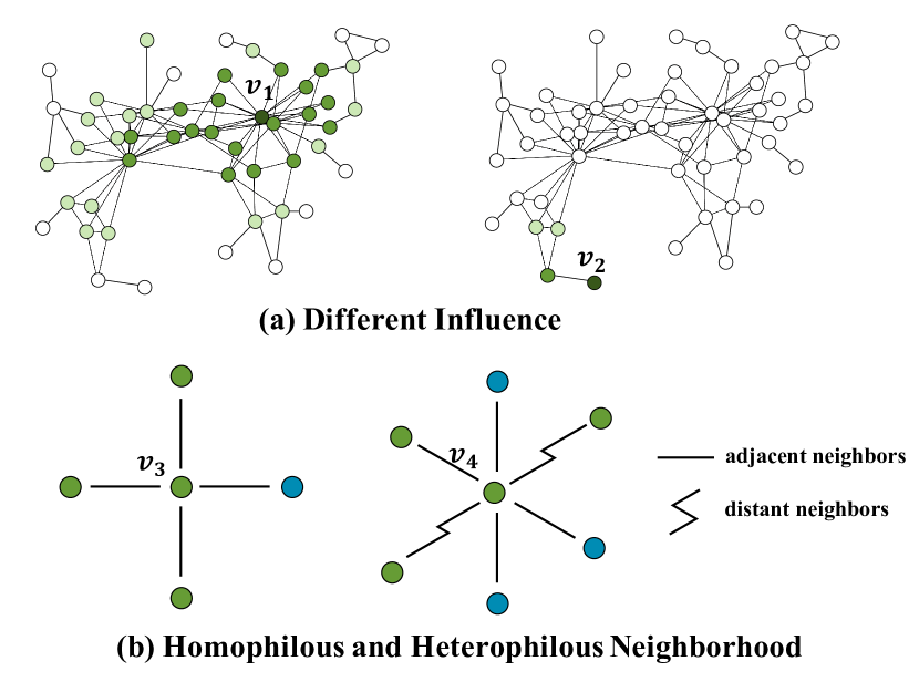
Figure 1. An illustration on node priority

In GNNs, the embedding of a node is learned by aggregating (propagating) messages from (to) its neighbors. Given a pre-set GNN layer $L$, for each node, it can perceive messages from neighbors that are $L$-hop away. With the increase of $L$, the receptive field of a node gets larger and more information can be aggregated from neighbors to generate the node’s embedding. However, due to the effect of low-pass convolutional filters used in GNNs, the embeddings of nodes in the same component of a graph tend to be indistinguishable with more layers stacked. This is the notorious over-smoothing (Rong et al., 2020) problem in GNNs. To tackle the problem, existing methods utilize various techniques, such as residual connection (Kipf and Welling, 2016), normalization schemes (Zhao and Akoglu, 2019) and boosting strategy (Sun et al., 2020). However, these methods treat all the nodes in the graph equally. Practically, nodes in the graph have various local structures. For example, in Facebook, some users play the role of hub, which link to many other users and are located at the center of a graph; some users are leaf nodes that have very few connections. Intuitively, nodes with fewer one-hop neighbors need to absorb messages from distant nodes for label prediction (Shi et al., 2020). However, an excessively large neighborhood range could lead to an over-smoothing problem. Further, it is infeasible to manually set propagation steps for all the nodes in the graph, which motivates the design of personalized node-wise message propagation layers.

Recently, some methods (Xu et al., 2018; Xiao et al., 2021; Wang et al., 2022) are proposed to learn node-wise message propagation in GNNs. However, most of these works distinguish node local structures only but ignore the different priorities of nodes. Specifically, assuming that a hub node is predicted incorrectly, it will then adversely infect a significant number of neighbors and easily contaminate the whole graph. Therefore, for hub nodes with high degrees, they are intuitively more influential than leaf nodes. For example, as shown in Figure 1(a), when we set the propagation step $L=2$, compared with the leaf node $v_{2}$, the hub node $v_{1}$ has a much larger receptive field, whose messages will propagate to and further influence more nodes in the graph; hence, we have to give higher priority to learning its message propagation. Also, it has been pointed out in (Chen et al., 2020) that nodes with higher degrees are more likely to suffer from over-smoothing with the increase of convolutional layers, which further provides evidence for giving larger priorities to high-degree nodes.

On the other hand, the priority of a node can also be reflected by its neighborhood. For a node with homophilous (Newman, 2002) neighborhood (see $v_{3}$ in Figure 1(b)), it tends to share similar characteristics or have the same label as its neighbors, so it is much easier to be classified with small message propagation steps. In contrast, for a node whose neighborhood is heterophilous (Newman, 2002) (see $v_{4}$ in Figure 1(b)), it is more likely to be connected with nodes that have dissimilar features or different labels. Therefore, its label prediction needs to collect information from distant multi-hop neighbors and thus requires a large message propagation step. Since nodes with heterophilous neighborhood are difficult to be classified, we have to pay more attention to those nodes in the learning process. To sum up, there arises a crucial question to make GNNs better: How to learn prioritized node-wise message propagation in GNNs?

In this paper, we learn Prioritized node-wise message Propagation in GNNs and propose the framework PPro. Specifically, PPro consists of three components: a backbone GNN model, a propagation controller and a weight controller, which are coupled with each other. For propagation controller, it is used to determine the optimal propagation steps for nodes. In particular, we design two strategies for propagation controller: L2B directly learns which step to break message propagation for a node, while L2U learns the best embedding of a node in all the pre-set steps and returns the corresponding propagation step. In both strategies, the controller functions consider node priority by taking factors that could affect node influence and heterophily as input. For the weight controller, it computes the priority scores for nodes, which takes into account the optimal propagation steps of nodes output by the propagation controller. After node priority scores are calculated, we integrate them with the widely used supervised loss function in GNNs. Note that our framework is easy-to-implement and can be plugged in with most existing GNN models. Finally, our main contributions in this paper are summarized as:

$\bullet$ We present a versatile framework PPro for learning prioritized node-wise message propagation in GNNs.

$\bullet$ We design a mutually enhanced mechanism to compute node priority, optimal propagation step and label prediction. We also propose an alternative optimization strategy to learn parameters.

$\bullet$ We conduct extensive experiments to verify the effectiveness of our proposed framework. In particular, we compare PPro with 11 other state-of-the-art methods on 8 benchmark datasets to show its superiority. We also implement PPro with various backbone GNN models to show its wide applicability.

2. Related Work

In this section, we summarize the related work on GNNs and learning to propagate in GNNs, respectively.

2.1. Graph Neural Networks

Recently, GNNs have received significant attention and there have been many GNN models proposed (Kipf and Welling, 2016; Wu et al., 2019; Veličković et al., 2017; Xu et al., 2019). Existing methods can be mainly divided into two categories: spectral model and spatial model. The former decomposes graph signals via graph Fourier transform and convolves on the spectral components, while the latter directly aggregates messages from a node’s spatially nearby neighbors. For example, the early model GCN (Kipf and Welling, 2016) extends the convolution operation to graphs and is in essence a spectral model. The representative spatial model GraphSAGE (Hamilton et al., 2017) aggregates information from a fixed size neighborhood of a node to generate its embedding. Graph attention networks (GATs) (Veličković et al., 2017) is also a spatial model, which employs the attention mechanism to learn the importance of an object’s neighbors and aggregate information from these neighbors with the learned weights. Despite the success, GNNs could suffer from the over-smoothing problem, where embeddings of nodes in the same component of a graph tend to be indistinguishable as the number of layers increases. To tackle the problem, existing methods utilize various techniques, such as residual connection (Kipf and Welling, 2016), normalization schemes (Zhao and Akoglu, 2019) and boosting strategy (Sun et al., 2020). There are also methods (Rong et al., 2020; Chen et al., 2018) that adopt graph augmentation to remove a proportion of nodes or edges in the graph to alleviate the problem. Recently, Klicpera et al. (2018) and Liu et al. (2020) present that the coupling of feature propagation and transformation causes the problem and they decouple the two steps to mitigate the effect of over-smoothing. Further, GCNII (Chen et al., 2020) proposes initial residual and identity mapping which can effectively boost the model performance.

Moreover, there are also many studies on designing GNNs for graphs with heterophily (Bo et al., 2021; Chien et al., 2021; Yan et al., 2021; Li et al., 2022; Zhu et al., 2020). For example, H₂GCN (Zhu et al., 2020) presents three strategies to improve the performance of GNNs under heterophily: ego and neighbor embedding separation, higher-order neighborhood utilization and intermediate representation combination. After that, based on the generalized PageRank, GPR-GNN (Chien et al., 2021) combines the low-pass and high-pass convolutional filters by adaptively learning the signed weights of node embeddings in each propagation layer. Further, to address the heterophily issue, Li et al. (2022) propose to find global homophily for each node by taking all the nodes in the graph as the node’s neighborhood. Our proposed framework models the priority of a node as a function of the heterophily degree of the node’s neighborhood, which can improve the performance of GNNs on heterophilous graphs.

2.2. Learning to Propagate in GNNs

Since different nodes in a graph may need a personalized number of propagation layers, learning to propagate in GNNs has recently attracted much attention. Although it can be used to alleviate the effect of over-smoothing, they are two different problems because learning to propagate targets at learning the propagation strategies of nodes. Currently, some methods (Xu et al., 2018; Xiao et al., 2021; Wang et al., 2022; Sun et al., 2020) have been proposed to learn message propagation in GNNs. For example, JKnet (Xu et al., 2018) presents an architecture that flexibly leverages different neighborhood ranges for each node to enable better structure-aware representation. Further, Xiao et al. (2021) present a general learning framework which can explicitly learn the interpretable and personalized propagation strategies for different nodes. Recently, Wang et al. (2022) present a framework that uses parametric controllers to decide the propagation depth for each node based on its local patterns. Although these works aim to learn personalized propagation strategies for each node, they ignore node priority that can be reflected by node influence and heterophily. This further motivates our study on prioritized node-wise message propagation.

3. Preliminary

In this section, we introduce the notations used in this paper and also some GNN basics.

3.1. Notations

Let $G=\mathcal{(V,E)}$ denote an undirected graph without self-loops, where $\mathcal{V}=\left\{v_{i}\right\}_{i=1}^{n}$ is a set of nodes and $\mathcal{E\subseteq V\times V}$ is a set of edges. Let $A$ be the adjacency matrix of $G$ such that $A_{ij}=1$ if there exists an edge between nodes $v_{i}$ and $v_{j}$; 0, otherwise. We denote the set of adjacent neighbors of node $v_{i}$ as $\mathcal{N}_{i}$. We further define a diagonal matrix $D$, where $D_{ii}=\textstyle\sum_{j=1}^{n}A_{ij}$ is the degree of node $v_{i}$. We use $X\in\mathbb{R}^{n\times d}$ to denote the node feature matrix, where the $i$-th row $X_{i}$ is the $d$-dimensional feature vector of node $v_{i}$. For the node representation matrix in the $k$-th layer, we denote it as $H^{(k)}$, where the $i$-th row $h_{i}^{(k)}$ is the corresponding embedding vector of node $v_{i}$. We also use $Y\in\mathbb{R}^{n\times c}$ to denote the ground-truth node label matrix, where $c$ is the number of labels. In this paper, we focus on the node-level classification task, where each node $v_{i}$ is associated with a label $y_{i}$.

3.2. Message Propagation

GNNs aggregate messages from a node’s neighborhood by different message propagation strategies. Generally, each propagation step in GNNs includes two sub-steps. We take an arbitrary node $v_{i}$ in the $k$-th layer as an example. The first sub-step is to aggregate information from a node’s neighbors, which is given as:

(1) $$\hat{h}_{i}^{(k)}=\texttt{AGGREGATE}(h_{j}^{(k-1)},\forall v_{j}\in\mathcal{N}_{i}).$$

After that, the second sub-step is to update node embeddings:

(2) $$h_{i}^{(k)}=\texttt{UPDATE}(h_{i}^{(k-1)},\hat{h}_{i}^{(k)}).$$

Many state-of-the-art GNN models follow this message propagation mechanism, such as GCN (Kipf and Welling, 2016) and GAT (Veličković et al., 2017). Further, there are also some methods that add the initial node embedding $h_{i}^{(0)}=f_{\theta}(X_{i})$ in the UPDATE function, such as APPNP (Klicpera et al., 2018) and GCNII (Chen et al., 2020). In this case, the UPDATE function should be modified into $h_{i}^{(k)}=\texttt{UPDATE}(h_{i}^{(k-1)},\hat{h}_{i}^{(k)},h_{i}^{(0)})$. After $L$ propagation steps, the final node embedding $h_{i}^{(L)}$ will be used in downstream tasks.

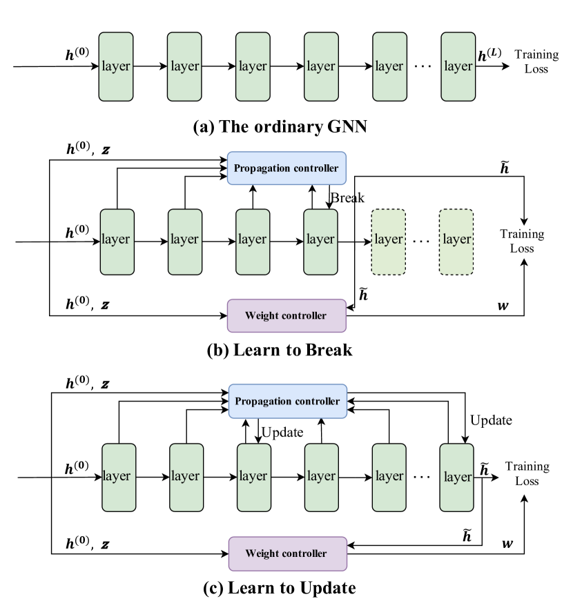
Figure 2. The overall framework of PPro. The propagation controller learns the propagation steps for nodes while the weight controller calculates the priority scores. (a) The general GNN pipeline; (b) Learning to break; (c) Learning to update

4. Method

In this section, we propose our framework PPro, which consists of a backbone GNN model, a propagation controller to learn propagation depth for nodes and a weight controller to learn node priority. We first introduce priority measures for nodes and then describe prioritized message propagation learning in propagation controller. After that, we show how to learn priority weights for nodes in weight controller. Finally, we present the optimization algorithm. The overall framework of PPro is summarized in Figure 2.

4.1. Priority Measures

As we discussed in Section 1, we would like to measure the priority of a node w.r.t. the degree of node influence and neighborhood heterogeneity. Specifically, we introduce three priority measures, including degree centrality, eigenvector centrality, and heterophily degree.

Degree Centrality. A node’s degree is the number of edges connected with it (in the undirected graphs). It is a measure for node centrality which is simple but effective (Newman, 2010). For example, for celebrities in social networks, they often connect with a significant number of neighbors and have higher influence than normal users. The degree centrality of node $v_{i}$ can be defined as:

(3) $$d_{i}={\textstyle\sum_{j=1}^{n}A_{ij}}.$$

Eigenvector Centrality. The eigenvector centrality is an extension to the degree centrality (Newman, 2010). Specifically, it measures the centrality of a node by distinguishing the importance of the node’s neighbors, while the degree centrality only considers equally important neighbors. The eigenvector centrality of a node is the weighted average of that of its neighbors, which is formally formulated as:

(4) $$ec_{i}={\textstyle\sum_{j=1}^{n}A_{ij}ec_{j}}.$$

Heterophily Degree. Given a node $v_{i}$ with heterophilous neighborhood, it usually needs a large propagation step to collect useful information from distant neighbors. Further, compared with nodes that have homophilous neighbors, the label of $v_{i}$ may be harder to predict and it should thus be given higher priority in the learning process. Therefore, we introduce heterophily degree as a measure of node priority, which is calculated by

(5) $$he_{i}=\left\|h_{i}^{(0)}-\hat{h}_{i}^{(1)}\right\|_{2},$$

where $\hat{h}_{i}^{(1)}=\texttt{AGGREGATE}(h_{j}^{(0)},\forall v_{j}\in\mathcal{N}_{i})$. Finally, we concatenate these three measures which are further used to learn propagation steps and priority weights in GNNs:

(6) $$z_{i}=\left[d_{i}\parallel ec_{i}\parallel he_{i}\right].$$

where $\parallel$ is the concatenation operator.

4.2. Propagation Controller

As shown in Figure 2(a), given a node with feature vector $h^{(0)}$ and a pre-set maximum propagation step $L$, GNNs aggregate messages from its neighbors by a propagation strategy and output the final representation $h^{(L)}$. However, it is inappropriate to set the same propagation step for all the nodes. Therefore, we propose a propagation controller to learn personalized propagation step for each node, which is implemented by two methods, namely, learning to break (L2B) and learning to update (L2U). In both methods, we use node priorities and the difference between a node’s representation and its neighbors’ in each layer to calculate node propagation steps. Next, we describe the details of both L2B and L2U.

L2B: The L2B method directly learns whether to break message propagation in a layer. Let $\mathcal{F}_{p}(\cdot;{\phi_{p}})$ be the propagation controller function with learnable parameters $\phi_{p}$. We also use ${r}_{b}^{(k)}\in\{0,1\}^{n}$ to denote whether to break aggregating for all the nodes in the $k$-th layer. We calculate the probability of node $v_{i}$ that breaks message aggregation in the $k$-th layer by :

(7) $$Pr(r_{bi}^{(k)}=1)=\mathcal{F}_{p}(z_{i},h_{i}^{(0)},h_{i}^{(k)},\hat{h}_{i}^{(k)};{\phi_{p}}),$$

where $z_{i}$ derived from Eq. 6 represents the priority of $v_{i}$, $h_{i}^{(0)}$ is $v_{i}$’s initial embedding and $\hat{h}_{i}^{(k)}=\texttt{AGGREGATE}(h_{j}^{(k-1)},\forall v_{j}\in\mathcal{N}_{i})$ is the representation of $v_{i}$’s neighborhood in the $k$-th step. After the probability is calculated, we introduce a hyper-parameter $\varepsilon$ as a threshold to control whether message propagation should break. Specifically, if $P({r}_{bi}^{(k)}=1)>\varepsilon$, we break information aggregation for $v_{i}$ from the $k$-th layer and obtain its final embedding $\tilde{h}_{i}=h^{(k)}_{i}$; otherwise, message propagation continues.

L2U: Different from L2B, L2U does not stop message propagation until it traverses all the $L$ steps. We overload $\tilde{h}_{i}$ as the best embedding of $v_{i}$ in all the traversed steps. In the $k$-th step, for node $v_{i}$, L2U judges whether node embedding $h^{(k)}_{i}$ is better than $\tilde{h}_{i}$. If yes, we update $\tilde{h}_{i}=h^{(k)}_{i}$ and record the corresponding propagation step $k$ for node $v_{i}$; otherwise, we keep $\tilde{h}_{i}$ unchanged. To characterize the advantage of $h^{(k)}_{i}$ over $\tilde{h}_{i}$, we add $\tilde{h}_{i}$ as an additional input to the propagation controller function $\mathcal{F}_{p}$. Formally, we use ${r}_{ui}^{(k)}\in\{0,1\}$ to represent whether to update $\tilde{h}_{i}$ in the $k$-th step. Then the probability to update $\tilde{h}_{i}$ is computed by:

(8) $$Pr({r}_{ui}^{(k)}=1)=\mathcal{F}_{p}(z_{i},h_{i}^{(0)},h_{i}^{(k)},\hat{h}_{i}^{(k)},\tilde{h}_{i};{\phi_{p}}).$$

After that, if $Pr({r}_{ui}^{(k)}=1)>\varepsilon$, we then update $\tilde{h}_{i}=h^{(k)}_{i}$. The above process is repeated until $L$ message propagation steps are performed. Finally, L2U sets the propagation step for node $v_{i}$ as the largest step where $\tilde{h}_{i}$ is updated. Note that, in both L2B and L2U, $\mathcal{F}_{p}$ can be implemented using MLP.

We design two different loss functions for L2B and L2U, respectively. For L2B, it learns whether to break message propagation in a given step. Intuitively, for a node that has a small prediction error, it is expected to stop message aggregation. Therefore, we normalize the prediction error and compare it with the probability of continuing message propagation. Formally, we define the loss for L2B as:

(9) $$\mathcal{L}_{p}^{b}=\frac{1}{m}{\textstyle\sum_{i=1}^{m}\left|\frac{C_{i}-C_{min}}{C_{max}-C_{min}}-Pr(r_{bi}^{(l_{i})}=0)\right|},$$

where $C_{i}=C(y_{i},\hat{y}_{i})$ and $C_{max},C_{min}$ is the max value and min value of $C$. Note that $l_{i}$ is the step to break the propagation for node $v_{i}$ and $r_{bi}^{(l_{i})}=0$ means to continue aggregation for $v_{i}$ in the $l_{i}$-th step. From Equation 9, when $C_{i}$ is small, $Pr(r_{bi}^{(l_{i})}=0)$ is also small, i.e., message should stop propagating; otherwise, $Pr(r_{bi}^{(l_{i})}=0)$ is large, which indicates that message should continue propagation.

For L2U, it learns the best embedding of a node in all the pre-set $L$ steps. Intuitively, for a node whose best embedding $\tilde{h}_{i}$ is to be updated with node embedding $h_{i}^{(k)}$ in the $k$-th step, it indicates that $Pr(r_{ui}^{(k)}=1)$ is large and the prediction error $C_{i}^{(k)}$ derived from $h_{i}^{(k)}$ should be smaller than the prediction error $\tilde{C}_{i}$ derived from $\tilde{h}_{i}$; otherwise, $Pr(r_{ui}^{(k)}=1)$ is small and $C_{i}^{(k)}$ should be larger than $\tilde{C}_{i}$. Hence, the loss function for L2U can be formulated as:

(10) $$\mathcal{L}_{p}^{u}=\frac{1}{m}{\textstyle\sum_{i=1}^{m}\frac{1}{L}{\textstyle\sum_{k=1}^{L}Pr(r_{ui}^{(k)}=1)(C_{i}^{(k)}-\tilde{C}_{i})}}.$$

For brevity, we use $\mathcal{L}_{p}$ to denote the loss function of propagation controller for both L2B and L2U in the following.

4.3. Weight Controller

To assign different priorities to nodes in the graph, we present an adaptive weight controller. On the one hand, the priority of a node is directly related to the measures given in Section 4.1. On the other hand, with the learning process, the propagation controller will output the corresponding propagation step for each node. Intuitively, the larger the propagation step, the more difficult a node to be classified, and the larger priority should be given. We also use node embeddings to help compute node priority. In particular, for node $v_{i}$, we use $h_{i}^{(0)}$ and $\tilde{h}_{i}$. Specifically, we define $\mathcal{F}_{w}(\cdot;\phi_{w})$ as the weighting function with learnable parameters $\phi_{w}$, and calculate the priority weight $w_{i}$ of a node $v_{i}$ by:

(11) $$w_{i}=\mathcal{F}_{w}(z_{i},h_{i}^{(0)},\tilde{h}_{i},l_{i};\phi_{w}),$$

where $l_{i}$ is the propagation step output by the propagation controller for node $v_{i}$. $\mathcal{F}_{w}$ can be implemented with MLP. After $w_{i}$ is computed, we inject it into the loss function used by GNN models. Given a backbone GNN model $\mathcal{F}_{g}$ with learnable parameters $\theta$, the general loss function in the supervised learning is given as

(12) $$\mathcal{L}_{g}=\frac{1}{m}{\textstyle\sum_{i=1}^{m}C(y_{i},\hat{y}_{i})},$$

where $\hat{y}_{i}=\mathcal{F}_{g}(x_{i};\theta)$ is the predicted label for node $v_{i}$, $y_{i}$ is the true label of $v_{i}$, and $C(y_{i},\hat{y}_{i})$ is a distance measure and $m$ is the training set size. With the weight $w_{i}$, we aim to minimize the reweighted loss function:

(13) $$\mathcal{L}_{g}=\max\limits_{w_{i}}\min\limits_{\theta}\frac{1}{m}{\textstyle\sum_{i=1}^{m}w_{i}C(y_{i},\hat{y}_{i})}-\lambda_{1}\frac{1}{m}{\textstyle\sum_{i=1}^{m}w_{i}^{2}}.$$

Here, the second term is $l_{2}$-norm and $\lambda_{1}$ is a hyper-parameter that controls the importance of the two terms.

4.4. Optimization

From the discussion above, we see that our framework has three learnable parameters: $\theta$, $\phi_{p}$ and $\phi_{w}$, which are coupled with each other. Both the two controllers take node embeddings output by the backbone GNN model as input, while the backbone GNN model depends on the two controllers to calculate priority weight and propagation step. Therefore, we adopt an alternating optimization strategy that optimizes each parameter with others fixed.

First, to optimize $\theta$, we fix $w_{i}$ in Equation 13 and directly calculate $\frac{\partial\mathcal{L}_{g}}{\partial\theta}$. Then for the weight controller, we fix $\theta$ and reduce Eq. 13 to $\mathcal{L}_{w}=\max\limits_{w_{i}}\frac{1}{m}{\textstyle\sum_{i=1}^{m}w_{i}C(y_{i},\hat{y}_{i})}-\lambda_{1}\frac{1}{m}{\textstyle\sum_{i=1}^{m}w_{i}^{2}}$. We compute $\frac{\partial\mathcal{L}_{w}}{\partial{\phi_{w}}}$ and adopt stochastic gradient ascent to optimize $\phi_{w}$. In this way, a large weight will be given to the node with large error prediction. Further, we fix $\theta$ and $\phi_{w}$, and optimize $\phi_{p}$ in $\mathcal{L}_{p}$.

Since weight controller and propagation controller share a large number of inputs and they are optimized alternatively, we implement them with a two-layer MLP in our experiments, where they share parameters in the first layer and have their own parameters in the second layer. We minimize the merged loss function of both controllers as:

(14) $$\mathcal{L}_{Controller}=\mathcal{L}_{p}-\lambda_{2}\mathcal{L}_{w},$$

where $\lambda_{2}$ is used to balance the two terms.

[Time complexity analysis]. Our proposed framework PPro can be integrated with any mainstream GNNs, which additionally introduces two controllers. Since the two controllers are implemented with a two-layer MLP, the time complexity of PPro is linear w.r.t. the number of nodes in the graph. Finally, we summarize the pseudocodes of our proposed framework PriPro in Algorithm 1 which can be found in Section A of the appendix.

5. EXPERIMENTS

This section comprehensively evaluates the performance of PPro against other state-of-the-art methods on benchmark datasets.

5.1. Experimental Settings

Datasets. We use 8 datasets in total, which can be divided into two groups. The first group is homophilous graphs, which include Cora, Citeseer and Pubmed. These datasets are three citation networks that are widely used for node classification (Yang et al., 2016). In these datasets, nodes represent publications and edges are citations between them. Further, node features are the bag-of-words representations of keywords contained in the publications. The other group of datasets is heterophilous graphs. We adopt five public datasets from (Pei et al., 2020): Actor, Chameleon, Cornell, Texas, Wisconsin. Specifically, Actor is a graph with heterophily, which represents actor co-occurrence in Wiki pages; for other datasets, they are web networks, where nodes are web pages and edges are hyperlinks. Statistics of these datasets are summarized in Table 6 of Section B in Appendix.

Baselines. To evaluate the effectiveness of PPro, we compare it with the SOTA GNN models, including GCN (Kipf and Welling, 2016), SGC (Wu et al., 2019), GAT (Veličković et al., 2017), JKnet (Xu et al., 2018), JKnet+ DropEdge (Rong et al., 2020) (JKnet (Drop)), APPNP (Klicpera et al., 2018), GCNII (Chen et al., 2020), GCNII^∗ (Chen et al., 2020), and two representative heterophilous-graph-oriented methods: H₂GCN (Zhu et al., 2020) and Geom-GCN (Pei et al., 2020). We further compare PPro with L2P (Xiao et al., 2021), which is the SOTA learn-to-propagate framework. For NW-GNN (Wang et al., 2022), while it can also learn personalized propagation for nodes, it focuses on the whole neural architecture search for various components in GNNs. Since its codes are not publicly available, we do not take it as our baseline for fairness. For our framework PPro, since we have two different strategies in the propagation controller, we name the corresponding frameworks as L2B and L2U for short, respectively. For fairness, we use APPNP as our backbone, which is the same as L2P (Xiao et al., 2021), and our framework is also applicable to other GNN models (Kipf and Welling, 2016; Wu et al., 2019; Veličković et al., 2017; Chen et al., 2020).

5.2. Performance Comparison with GNNs

We first conduct experiments to compare PPro with other GNN models on both homophilous and heterophilous graphs.

Performance on homophilous graphs. We use the standard fixed training/validation/testing splits (Kipf and Welling, 2016) on three datasets Cora, Citeseer, and Pubmed, with 20 nodes per class for training, 500 nodes for validation and 1,000 nodes for testing, respectively. Table 1 reports the mean classification accuracy on the test set after 10 runs. From the table, we make the following observations: (1) Our methods L2B and L2U perform very well on all the datasets. In particular, L2B achieves the best results on both Citeseer and Pubmed. While it is not the winner on Cora, the performance gap with the best result is marginal. (2) Compared with the backbone model APPNP, our frameworks L2B and L2U can consistently improve its performance on all three datasets. All these results show the effectiveness of PPro on homophilous graphs.

Table 1. Node classification accuracy ($\%$) on homophilous graphs. We highlight the best score for each dataset in bold.

Method	Cora	Citeseer	Pubmed
GCN	81.5	70.3	79.0
SGC	81.0	71.9	78.9
GAT	83.0	72.5	79.0
JKNet	81.1	69.8	78.1
JKNet (Drop)	83.3	72.6	79.2
APPNP	83.3	71.8	80.1
GCNII	85.5	73.4	80.2
GCNII∗	85.3	73.2	80.3
L2B	$85.0\pm 0.8$	$\textbf{74.0}\pm 0.8$	$\textbf{81.1}\pm 0.4$
L2U	$85.0\pm 0.4$	$72.7\pm 0.9$	$81.1\pm 0.5$

Performance on heterophily graphs. Table 2 shows the mean classification accuracy of all the models on heterophilous graphs. Here, we use four datasets: Chameleon, Cornell, Texas and Wisconsin. For each dataset, we randomly split nodes of each class into 60%, 20%, and 20% for training, validation and testing, respectively. We measure the model performance on the test sets over 10 random splits as suggested in (Pei et al., 2020). From the table, we see that (1) Our framework can consistently lead to the best results on all the datasets. In particular, L2B is the winner for three cases while L2U beats others on Wisconsin. (2) Our framework shows superiority over H₂GCN and Geom-GCN, which are specially designed for graphs with heterophily. (3) Both L2B and L2U significantly improve APPNP on heterophilous graphs. These results show that even in heterophilous graphs, our framework can still work well. This is because we give high priorities to nodes with heterophilous neighborhood that are difficult to classify in the learning process.

Table 2. Node classification accuracy ($\%$) on heterophilous graphs. For each dataset, we highlight the best result in bold.

Method	Chameleon	Cornell	Texas	Wisconsin
GCN	28.18	52.70	52.16	45.88
GAT	42.93	54.32	58.38	49.41
JKNet	60.07	57.30	56.49	48.82
JKNet (Drop)	62.08	61.08	57.30	50.59
APPNP	54.30	73.51	65.41	69.02
GCNII	60.61	74.86	69.46	74.12
GCNII∗	62.48	76.49	77.84	81.57
H2GCN	57.11	82.16	84.86	86.67
Geom-GCN	60.90	60.81	67.57	64.12
L2B	63.68	86.22	85.67	$85.29$
L2U	$54.42$	$84.32$	$85.67$	86.86

Performance with other backbones. To further show the effectiveness of our framework, we use other GNN models as backbone, including GCN (Kipf and Welling, 2016), GAT (Veličković et al., 2017) and GCNII (Chen et al., 2020). Table 3 reports the classification results. From the table, we see that both L2B and L2U can consistently improve the performance of GCN and GAT on all three datasets. For GCNII, while it is the state-of-the-art GNN model, L2B can also enhance its performance on Citeseer and Pubmed. We further notice that L2U is outperformed by GCNII. This could be explained by the fact that GCNII adopts the initial residual and identity mapping techniques to preserve the initial features and information in previous layers for each node in each propagation layer. This leads to a small difference between node embeddings in consecutive propagation layers, which increases the difficulty for L2U to predict the layer to be selected and adversely affect its performance. In general, our framework can work well with other backbone models, which demonstrates its effectiveness.

Table 3. Node classification accuracy ($\%$) on homophilous graphs with other backbones.

Method	Cora	Citeseer	Pubmed
GCN	81.5	70.3	79.0
L2B	82.6	73.3	79.5
L2U	82.7	72.7	79.4
GAT	83.0	72.5	79.0
L2B	83.3	73.0	79.0
L2U	83.2	73.6	79.7
GCNII	85.5	73.4	80.2
L2B	84.6	73.9	80.4
L2U	84.2	72.6	79.8

5.3. Over-smoothing

To evaluate the effectiveness of our proposed framework for alleviating the over-smoothing problem, we study how L2B and L2U perform as the number of layers increases compared to other state-of-the-art GNNs. Table 4 summarizes the classification results. We vary the number of layers from $\left\{2,4,8,16,32,64\right\}$. From the table, it is clear that, as the number of propagation steps increases, the performance of GCN drops rapidly, while both L2B and L2U can consistently perform well on all three datasets. Although GCNII can also alleviate over-smoothing, its performance in small propagation steps is poor. For example, with two propagation steps, CGNII achieves an accuracy of $68.2$ only on Citeseer, while that of L2B is $72.9$. This shows that our proposed framework can lead to more stable model performance in various propagation steps.

Table 4. Node classification accuracy ($\%$) on homophilous graphs with different propagation steps. For each method, we highlight its best score among all the layers in bold.

Datasets	Method	Propagation steps
		2	4	8	16	32	64
Cora	GCN	81.5	80.4	69.5	64.9	60.3	28.7
	JKNet	-	80.2	80.7	80.2	81.1	71.5
	JKNet (Drop)	-	83.3	82.6	83.0	82.5	83.2
	GCNII	82.2	82.6	84.2	84.6	85.4	85.5
	GCNII∗	80.2	82.3	82.8	83.5	84.9	85.3
	L2B	82.9	84.1	85.0	84.6	84.8	84.6
	L2U	83.2	84.2	84.6	84.7	85.0	84.5
Citeseer	GCN	70.3	67.6	30.2	18.3	25.0	20.0
	JKNet	-	68.7	67.7	69.8	68.2	63.4
	JKNet (Drop)	-	72.6	71.8	72.6	70.8	72.2
	GCNII	68.2	68.9	70.6	72.9	73.4	73.4
	GCNII∗	66.1	67.9	70.6	72.0	73.2	73.1
	L2B	72.9	73.4	73.4	74.0	73.4	72.0
	L2U	71.5	71.5	72.3	72.6	72.7	72.4
Pubmed	GCN	79.0	76.5	61.2	40.9	22.4	35.3
	JKNet	-	78.0	78.1	72.6	72.4	74.5
	JKNet (Drop)	-	78.7	78.7	79.1	79.2	78.9
	GCNII	78.2	78.8	79.3	80.2	79.8	79.7
	GCNII∗	77.7	78.2	78.8	80.3	79.8	80.1
	L2B	79.9	80.4	80.7	81.1	80.6	80.9
	L2U	79.5	80.3	80.7	81.1	80.7	80.1

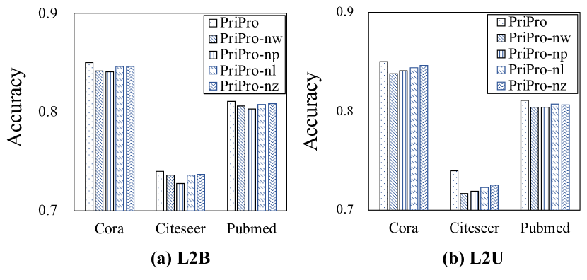
Figure 3. Ablation study

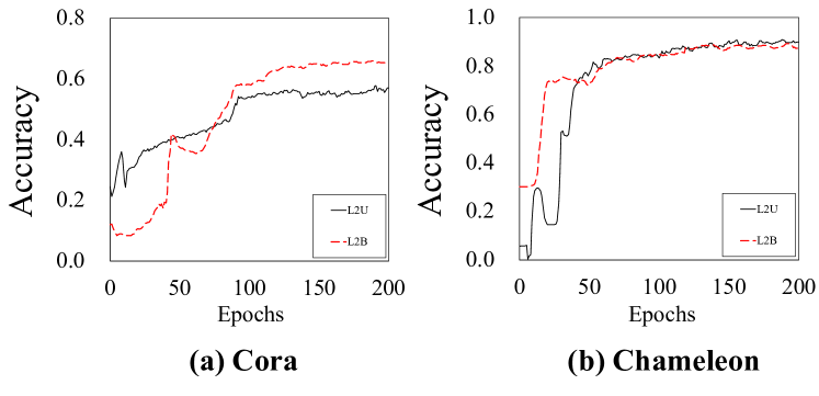
Figure 4. Convergence analysis

5.4. Performance Comparison with Other Framework

We further compare the performance of PPro with L2P, which is the state-of-the-art framework for learning node-wise message propagation. Specifically, it uses two different strategies, namely, learning to quit (L2Q) and learning to select (L2S) to learn optimal propagation steps for nodes, We first recap the difference between our proposed framework PPro and L2P: for L2B and L2Q, both of them aim to learn whether to stop in a specific step, but L2B considers node priority; both L2U and L2S learn in which step the node embedding should be selected as the final node representation in a maximum of $L$ steps. However, L2S formulates the problem as a multi-class classification one, which directly outputs the label (step) from $L$ class labels (steps), while L2U performs binary classification in each step. For fairness, we take APPNP as the backbone model for both frameworks, and directly report the results of L2S and L2Q from the original paper. Table 5 illustrates the classification results. From the table, we see that the PPro framework leads to the best results in 5 out of 7 datasets, which verifies the importance of incorporating node priority in learning node-wise message propagation. In particular, PPro outperforms L2P on all heterophilous graphs, which shows the effectiveness of giving high priorities to nodes with high heterophily. Further, L2U generally performs better than L2S. This could be because when $L$ is large and labeled data is scarce, it is difficult to directly perform $L$-class classification.

Table 5. Performance Comparison with L2P. For each dataset, we highlight the best result in bold.

Framework	Method	Datasets
		Cora	Citeseer	Pubmed	Actor	Cornell	Texas	Wisconsin
L2P	L2Q	85.2	74.6	80.4	37.0	81.1	84.6	84.7
	L2S	84.9	74.2	80.2	36.6	80.5	84.1	84.3
PPro	L2B	85.0	74.0	81.1	36.8	86.2	85.7	85.3
	L2U	85.0	72.7	81.1	37.1	84.6	85.7	86.9

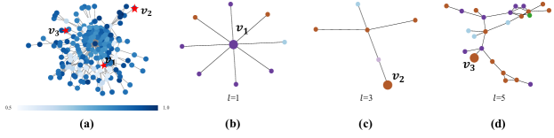
Figure 5. The visualization on the node priority weights and propagation steps calculated by L2B. In (b)-(d), we show the subgraphs centered at $v_{1}$, $v_{2}$ and $v_{3}$, respectively. Different colors represent node labels. Better view in color.

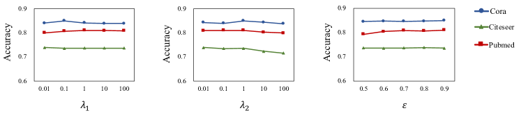
Figure 6. Hyper-parameter sensitivity analysis

5.5. Ablation Study

We next conduct an ablation study to understand the main components of PriPro, which consists of a backbone GNN model, a propagation controller and a weight controller. Specifically, the propagation controller computes the optimal propagation step for each node considering node priority, while the weight controller calculates the node priority scores by taking into account the optimal propagation steps of nodes. We first remove the optimal propagation step as input from the weight controller and call this variant PPro-nl (no propagation step $l$). Similarly, we remove the node priority as input from the propagation controller and call this variant PPro-nz (no node priority $z$). Further, we remove the weight controller and the propagation controller, and call these variants PPro-nw (no weight controller) and PPro-np (no propagation controller), respectively. Finally, we compare L2B and L2U with these variants and show the results in Figure 3. From the figure, we see that (1) PPro clearly outperforms all the variants on the three datasets. (2) The performance gap between PPro and PPro-nw (PPro-np) shows the importance of the weight controller (propagation controller) in learning node-wise message propagation. (3) PPro performs better than PPro-nl (PPro-nz), which shows that the optimal node propagation steps (node priority) can help learn better node priority (optimal node propagation steps) and further boost the model performance.

5.6. Convergence Analysis

We next analyze the convergence of PPro during the learning process. We conduct experiments on two datasets: Cora and Chameleon. For other datasets, we observe similar results, which are omitted due to the space limitation. We show the accuracy scores of both L2B and L2U on the validation set with increasing epochs in Figure 4. For both methods, we use the same training/validation set on each dataset and run the experiments for 200 epochs. From the figure, we see that both L2B and L2U converge fast. We speculate that this is because our proposed framework implements both controllers with a two-layer MLP. The simple network structure of MLP mitigates the difficulty of model training, which further facilitates model convergence.

5.7. Node Priority and Propagation Step

To evaluate if PPro can well learn node-wise priority and propagation steps, we visualize the results given by the weight controller and the propagation controller, respectively. Figure 5(a) shows the priority scores of nodes calculated by the weight controller of L2B. For ornamental purposes, we take Cornell as an example, which has a small number of nodes and is easy to visualize. For all the nodes, the darker the color, the larger the weight. From the figure, we find that the high-degree nodes tend to have large priority scores. This is consistent with our assignment of large priority for nodes with high influence. Further, we see that some leaf nodes with few links in the graph are also given large weights. Since Cornell is a heterophilous graph, these leaf nodes are often difficult to gather useful information from neighborhood. This is also consistent with that we would like to focus more on nodes that are difficult to predict. Figure 5(b)-(d) further shows some case studies from Cornell on the learned node propagation steps, where different colors represent node labels. In Figure 5(b), node $v_{1}$ has homophilous neighborhood where most adjacent neighbors are in the same label, so 1-hop message aggregation is sufficient for label prediction. Compared with node $v_{1}$, node $v_{2}$ in Figure 5 needs a larger propagation step due to its higher heterophily. For node $v_{3}$ in Figure 5(d), since its neighborhood is of large heterophily, it needs a large propagation step $l=5$ to absorb useful information from distant nodes in the same label. All these results demonstrate the effectiveness of the weight controller and the propagation controller in PPro.

5.8. Hyperparameter Sensitivity Analysis

We end this section with a sensitivity analysis on the hyperparameters of PPro. In particular, we study three key hyperparameters: the regularization weight $\lambda_{1}$, the balance coefficient $\lambda_{2}$, and a threshold $\varepsilon$. In our experiments, we vary one parameter each time with others fixed. Figure 6 illustrates the results of L2B on Cora, Citeseer and Pubmed w.r.t. classification accuracy. From the figure, we see that for all three hyper-parameters, L2B can give very stable performances over a wide range of hyperparameter values. The threshold $\epsilon$ determines the likelihood to break the propagation process. The larger the threshold, the easier to propagate more layers. Since PPro can effectively alleviate the over-smoothing problem, increasing the threshold allows more steps to propagate, which would not affect the classification results too much. All the results show the insensitivity of PPro w.r.t. these hyper-parameters.

6. CONCLUSIONS

In this paper, we learned prioritized node-wise message propagation in GNNs and proposed the framework PriPro. The framework consists of three components: a backbone GNN model, a propagation controller to determine the optimal propagation steps for nodes, and a weight controller to compute the priority scores for nodes. We designed a mutually enhanced mechanism to compute node priority, optimal propagation step and label prediction. We conducted extensive experiments and compared PriPro with 11 other methods. Our analysis shows that PriPro is very effective and can lead to superior classification performance.

Appendix A ALGORITHM

We summarize the pseudocodes of our proposed framework PPro in Algorithm 1.

Input: Graph $G=\mathcal{(V,E)}$, learning rate $\alpha_{g},\alpha_{\mathcal{F}}$, epoch $T$, max aggregation step $L$.

Output: learned prameters $\theta,\phi$.

1 Randomly initialize $\theta^{(0)},\phi^{(0)}$;

2 for $t=0,1,...,T-1$ do

3       $\tilde{h}=h^{(0)}$;

4       for $k=1,2,...,L$ do

5             $h^{(k)}=\texttt{GNN}(h^{(k-1)},\theta^{(t)})$

6             $Pr(r^{(k)}=1)=\mathcal{F}_{p}(\cdot;\phi_{p}^{(t)})$

7             $\tilde{h}\leftarrow Pr(r^{(k)}=1),h^{(k)}$

8            

9      $w=\mathcal{F}_{w}(\cdot;\phi_{w}^{(t)})$

10       $\theta^{(t+1)}=\theta^{(t)}-\alpha_{g}\nabla_{\theta}\mathcal{L}_{g}$

11       repeat 3-9 with the parameter $\theta^{(t+1)}$

12       $\phi^{(t+1)}=\phi^{(t)}-\alpha_{\mathcal{F}}\nabla_{\phi}\mathcal{L}_{Controller}$

13      

return $\phi$ and $\theta$

Algorithm 1 PPro

Appendix B DATASETS

In our experiments, we use the following real-world datasets, whose details are given as follows. Statistics of these datasets are summarized in Table 6.

Cora, Citeseer and Pubmed are three homophilous graphs which are broadly applied as benchmarks. In these datasets, each node represents a scientific paper and each edges represents a citation. These graphs use bag-of-words representations as the feature vector for each node. Each node is assigned a label indicating the research field. The task on these datasets is node classification.

Texas, Wisconsin and Cornell are three heterophilous graphs which representing links between web pages of the corresponding universities. In these datasets, each node represents a web page and each edge represents a hyperlink between nodes. We take bag-of-words representations as a feature vector for each node. The task on these datasets is node classification.

Chameleon is a subgraph of web pages in Wikipedia. The task is to classify the nodes into five categories. Note that this dataset is heterophilous graphs.

Actor is a heterophilous graph which represents actor co-occurrence in Wiki pages. Node features are built from the keywords that are included in the actor’s Wikipedia page. Our task was to divide the actors into five classes.

Table 6. Datasets statistics.

Dataset	Classes	Nodes	Edges	Features
Cora	7	2,708	5,429	1,433
Citeseer	6	3,327	4,732	3,703
Pubmed	3	19,717	44,338	500
Actor	5	7,600	26,659	932
Chameleon	5	2,277	36,101	2,325
Cornell	5	183	295	1,703
Texas	5	183	309	1,703
Wisconsin	5	251	499	1,703

Appendix C Implementation Details

We implement PPro by PyTorch and optimize the framework by Adam (Kingma and Ba, 2014). For fairness, we use APPNP as our backbone, which is the same as L2P (Xiao et al., 2021), and our framework is also applicable to other GNN models (Kipf and Welling, 2016; Wu et al., 2019; Veličković et al., 2017; Chen et al., 2020). We perform a grid search to fine-tune hyper-parameters based on the results on the validation set. Details on the search space can be found in Table 7. Further, since the results of most baseline methods on these benchmark datasets are public, we directly report these results from their original papers. For those cases where the results are missing, we report their results from (Chen et al., 2020). We run all the experiments on a server with 32G memory and a single Tesla V100 GPU.

Table 7. Grid search space.

Hyperparameter	Search space
lr	$\{0.005,0.01,0.05,0.1\}$
dropout	$[0,0.9]$
early stopping	$\{100,200\}$
weight decay	{1e-5, 5e-4, 1e-4, 5e-3, 1e-3 }
$\lambda_{1}$	$\{0.01,0.1,1,10^{1},10^{2}\}$
$\lambda_{2}$	$\{0.01,0.1,1,10^{1},10^{2}\}$
$\varepsilon$	$[0.1,0.9]$

References

- (1)
- Bo et al. (2021) Deyu Bo, Xiao Wang, Chuan Shi, and Huawei Shen. 2021. Beyond Low-frequency Information in Graph Convolutional Networks. In AAAI. AAAI Press.
- Chen et al. (2018) Jie Chen, Tengfei Ma, and Cao Xiao. 2018. Fastgcn: fast learning with graph convolutional networks via importance sampling. arXiv preprint arXiv:1801.10247 (2018).
- Chen et al. (2020) Ming Chen, Zhewei Wei, Zengfeng Huang, Bolin Ding, and Yaliang Li. 2020. Simple and deep graph convolutional networks. In International Conference on Machine Learning. PMLR, 1725–1735.
- Chien et al. (2021) Eli Chien, Jianhao Peng, Pan Li, and Olgica Milenkovic. 2021. Adaptive Universal Generalized PageRank Graph Neural Network. In International Conference on Learning Representations. https://openreview.net/forum?id=n6jl7fLxrP
- Hamilton et al. (2017) Will Hamilton, Zhitao Ying, and Jure Leskovec. 2017. Inductive representation learning on large graphs. Advances in neural information processing systems 30 (2017).
- Hogan et al. (2020) Aidan Hogan, Eva Blomqvist, Michael Cochez, Claudia d’Amato, Gerard de Melo, Claudio Gutiérrez, José Emilio Labra Gayo, Sabrina Kirrane, Sebastian Neumaier, Axel Polleres, Roberto Navigli, Axel-Cyrille Ngonga Ngomo, Sabbir M. Rashid, Anisa Rula, Lukas Schmelzeisen, Juan F. Sequeda, Steffen Staab, and Antoine Zimmermann. 2020. Knowledge Graphs. CoRR abs/2003.02320 (2020). arXiv:2003.02320 https://arxiv.org/abs/2003.02320
- Kingma and Ba (2014) Diederik P Kingma and Jimmy Ba. 2014. Adam: A method for stochastic optimization. arXiv preprint arXiv:1412.6980 (2014).
- Kipf and Welling (2016) Thomas N Kipf and Max Welling. 2016. Semi-supervised classification with graph convolutional networks. arXiv preprint arXiv:1609.02907 (2016).
- Klicpera et al. (2018) Johannes Klicpera, Aleksandar Bojchevski, and Stephan Günnemann. 2018. Predict then propagate: Graph neural networks meet personalized pagerank. arXiv preprint arXiv:1810.05997 (2018).
- Leskovec et al. (2010) Jure Leskovec, Daniel Huttenlocher, and Jon Kleinberg. 2010. Predicting positive and negative links in online social networks. In Proceedings of the 19th international conference on World wide web. 641–650.
- Li and Goldwasser (2019) Chang Li and Dan Goldwasser. 2019. Encoding social information with graph convolutional networks forpolitical perspective detection in news media. In Proceedings of the 57th Annual Meeting of the Association for Computational Linguistics. 2594–2604.
- Li et al. (2022) Xiang Li, Renyu Zhu, Yao Cheng, Caihua Shan, Siqiang Luo, Dongsheng Li, and Weining Qian. 2022. Finding Global Homophily in Graph Neural Networks When Meeting Heterophily. arXiv preprint arXiv:2205.07308 (2022).
- Liu et al. (2020) Meng Liu, Hongyang Gao, and Shuiwang Ji. 2020. Towards deeper graph neural networks. In Proceedings of the 26th ACM SIGKDD international conference on knowledge discovery & data mining. 338–348.
- Liu et al. (2021) Yixin Liu, Zhao Li, Shirui Pan, Chen Gong, Chuan Zhou, and George Karypis. 2021. Anomaly detection on attributed networks via contrastive self-supervised learning. IEEE transactions on neural networks and learning systems 33, 6 (2021), 2378–2392.
- Newman (2010) Mark Newman. 2010. Networks: An Introduction. Oxford University Press. https://doi.org/10.1093/acprof:oso/9780199206650.001.0001
- Newman (2002) Mark EJ Newman. 2002. Assortative mixing in networks. Physical review letters 89, 20 (2002), 208701.
- Pei et al. (2020) Hongbin Pei, Bingzhe Wei, Kevin Chen-Chuan Chang, Yu Lei, and Bo Yang. 2020. Geom-gcn: Geometric graph convolutional networks. arXiv preprint arXiv:2002.05287 (2020).
- Rong et al. (2020) Yu Rong, Wenbing Huang, Tingyang Xu, and Junzhou Huang. 2020. DropEdge: Towards Deep Graph Convolutional Networks on Node Classification. In International Conference on Learning Representations. https://openreview.net/forum?id=Hkx1qkrKPr
- Shi et al. (2020) Yunsheng Shi, Zhengjie Huang, Wenjin Wang, Hui Zhong, Shikun Feng, and Yu Sun. 2020. Masked Label Prediction: Unified Massage Passing Model for Semi-Supervised Classification. CoRR abs/2009.03509 (2020). arXiv:2009.03509 https://arxiv.org/abs/2009.03509
- Sun et al. (2020) Ke Sun, Zhanxing Zhu, and Zhouchen Lin. 2020. AdaGCN: Adaboosting Graph Convolutional Networks into Deep Models. In International Conference on Learning Representations.
- Veličković et al. (2017) Petar Veličković, Guillem Cucurull, Arantxa Casanova, Adriana Romero, Pietro Lio, and Yoshua Bengio. 2017. Graph attention networks. arXiv preprint arXiv:1710.10903 (2017).
- Wang et al. (2022) Zhen Wang, Zhewei Wei, Yaliang Li, Weirui Kuang, and Bolin Ding. 2022. Graph Neural Networks with Node-wise Architecture. In Proceedings of the 28th ACM SIGKDD Conference on Knowledge Discovery and Data Mining. 1949–1958.
- Wu et al. (2019) Felix Wu, Amauri Souza, Tianyi Zhang, Christopher Fifty, Tao Yu, and Kilian Weinberger. 2019. Simplifying graph convolutional networks. In International conference on machine learning. PMLR, 6861–6871.
- Xiao et al. (2021) Teng Xiao, Zhengyu Chen, Donglin Wang, and Suhang Wang. 2021. Learning how to propagate messages in graph neural networks. In Proceedings of the 27th ACM SIGKDD Conference on Knowledge Discovery & Data Mining. 1894–1903.
- Xu et al. (2019) Keyulu Xu, Weihua Hu, Jure Leskovec, and Stefanie Jegelka. 2019. How Powerful are Graph Neural Networks?. In International Conference on Learning Representations. https://openreview.net/forum?id=ryGs6iA5Km
- Xu et al. (2018) Keyulu Xu, Chengtao Li, Yonglong Tian, Tomohiro Sonobe, Ken-ichi Kawarabayashi, and Stefanie Jegelka. 2018. Representation learning on graphs with jumping knowledge networks. In International conference on machine learning. PMLR, 5453–5462.
- Yan et al. (2021) Yujun Yan, Milad Hashemi, Kevin Swersky, Yaoqing Yang, and Danai Koutra. 2021. Two Sides of the Same Coin: Heterophily and Oversmoothing in Graph Convolutional Neural Networks. CoRR abs/2102.06462 (2021). arXiv:2102.06462 https://arxiv.org/abs/2102.06462
- Yang et al. (2016) Zhilin Yang, William Cohen, and Ruslan Salakhudinov. 2016. Revisiting semi-supervised learning with graph embeddings. In International conference on machine learning. PMLR, 40–48.
- Ying et al. (2018) Rex Ying, Ruining He, Kaifeng Chen, Pong Eksombatchai, William L. Hamilton, and Jure Leskovec. 2018. Graph Convolutional Neural Networks for Web-Scale Recommender Systems. CoRR abs/1806.01973 (2018). arXiv:1806.01973 http://arxiv.org/abs/1806.01973
- Zhao and Akoglu (2019) Lingxiao Zhao and Leman Akoglu. 2019. Pairnorm: Tackling oversmoothing in gnns. arXiv preprint arXiv:1909.12223 (2019).
- Zhu et al. (2020) Jiong Zhu, Yujun Yan, Lingxiao Zhao, Mark Heimann, Leman Akoglu, and Danai Koutra. 2020. Beyond homophily in graph neural networks: Current limitations and effective designs. Advances in Neural Information Processing Systems 33 (2020), 7793–7804.
- Zitnik and Leskovec (2017) Marinka Zitnik and Jure Leskovec. 2017. Predicting multicellular function through multi-layer tissue networks. Bioinformatics 33, 14 (2017), i190–i198.