Electroweak baryogenesis, dark matter, and dark CP-symmetry

Abstract

With the motivation of explaining the dark matter and achieving the electroweak baryogenesis via the spontaneous CP-violation at high temperature, we propose a complex singlet scalar ($S=\frac{\chi+i\eta_{s}}{\sqrt{2}}$) extension of the two-Higgs-doublet model respecting a discrete dark CP-symmetry: $S\to-S^{*}$. The dark CP-symmetry guarantees $\chi$ to be a dark matter candidate on one hand and on the other hand allows $\eta_{s}$ to have mixings with the pseudoscalars of the Higgs doublet fields, which play key roles in generating the CP-violation sources needed by the electroweak baryogenesis at high temperature. The universe undergoes multi-step phase transitions, including a strongly first-order electroweak phase transition during which the baryon number is produced. At the present temperature, the observed vacuum is produced and the CP-symmetry is restored so that the stringent electric dipole moment experimental bounds are satisfied. Considering relevant constraints, we study the simple scenario of $m_{\chi}$ around the Higgs resonance region, and find that the dark matter relic abundance and the baryon asymmetry can be simultaneously explained. Finally, we briefly discuss the gravitational wave signatures at future space-based detectors and the LHC signatures.

I Introduction

The baryon asymmetry of the universe (BAU) presents one of the major quests for particle cosmology. By the observation based on the Big-Bang Nucleosynthesis, the BAU is pdg2020

$$Y_{B}\equiv\rho_{B}/s=(8.2-9.2)\times 10^{-11},$$ (1)

where $\rho_{B}$ is the baryon number density and $s$ is the entropy density. Three necessary Sakharov conditions have to be fulfilled for a dynamical generation of BAU: baryon number changing interactions, non-conservation of C and CP, and departure from thermal equilibrium Sakharov . The electroweak baryogenesis (EWBG) ewbg1 ; ewbg2 provides a promising and attractive mechanism of explaining the BAU since it is testable at the energy frontier by the LHC and at the precision frontier by the electric dipole moment (EDM) experiments. To realize the EWBG, one needs extend the SM to produce sufficient large CP-violation and a strongly first-order electroweak phase transition (EWPT), such as the singlet extension of SM (see e.g. bgs-1 ; bgs-3 ; bgs-4 ; bgs-5 ; bgs-6 ; Beniwal:2018hyi ; Huang:2018aja ; Ghorbani:2017jls ; cao ; huang ; Xie:2020wzn ; Ellis:2022lft ; Lewicki:2021pgr ; Idegawa:2023bkh ; Harigaya:2022ptp ) and the two-Higgs-doublet model (2HDM) (see e.g. bg2h-1 ; bg2h-2 ; bg2h-3 ; Kanemura:2004ch ; Basler:2017uxn ; Abe:2013qla ; bg2h-5 ; bg2h-4 ; bg2h-6 ; bg2h-7 ; bg2h-8 ; bg2h-9 ; bg2h-11 ; Basler:2020nrq ; bg2h-13 ; bg2h-12 ; 2111.13079 ; 2207.00060 ; Goncalves:2023svb ).

The negative results in the EDM searches for electrons impose stringent constraints on the explicit CP-violation interactions in the scalar couplings and Yukawa couplings edm-e . There are some cancellation mechanisms of CP-violation effects in the EDM, which can relax the tension between the EWBG and the EDM data 1411.6695 ; Fuyuto:2017ewj ; Modak:2018csw ; Fuyuto:2019svr ; Modak:2020uyq ; 2004.03943 ; 2111.13079 ; 2207.00060 . Even with the cancellation, there are several CP observables of radiative $B$ meson decays that still provide stringent constraints, such as the asymmetry of the CP-asymmetry of inclusive $B\to X_{s}\gamma$ decay Modak:2018csw ; Modak:2020uyq , Alternatively, a finite temperature spontaneous CP-violation mechanism is naturally compatible with the EDM data, where the CP symmetry is spontaneously broken at the high temperature and it is recovered at the present temperature. The novel mechanism was achieved in the singlet scalar extension of the SM cao ; huang in which a high dimension effective operator needs to be added, and the singlet pseudoscalar extension of 2HDM Huber:2022ndk ; Liu:2023sey .

In addition to the BAU, the dark matter (DM) is one of the longstanding questions of particle physics and cosmology. In this paper, we propose a complex singlet scalar extension of the 2HDM respecting a discrete dark CP-symmetry, and simultaneously explain the observed DM relic density and the BAU via the spontaneous CP-violation at high temperature. The dark CP-symmetry allows the imaginary component of singlet scalar to have mixings with the pseudoscalars of scalar doublet fields, which play key roles in generating the CP-violation sources needed by the EWBG at high temperature. On the other hand, the dark CP-symmetry guarantees the real component to be a DM candidate.

II 2HDM + $S$ respecting a dark CP-symmetry

Imposing a discrete dark CP-symmetry, we extend the SM by a second Higgs doublet $\Phi_{2}$ and a complex singlet $S$,

$$\Phi_{1}=\left(\begin{array}[]{c}\phi_{1}^{+}\\ \frac{(v_{1}+\rho_{1}+i\eta_{1})}{\sqrt{2}}\end{array}\right)\,,\Phi_{2}=\left(\begin{array}[]{c}\phi_{2}^{+}\\ \frac{(v_{2}+\rho_{2}+i\eta_{2})}{\sqrt{2}}\end{array}\right),S=\frac{(\chi+i\eta_{s})}{\sqrt{2}},$$ (6)

with $v_{1}$ and $v_{2}$ being the vacuum expectation values (VEVs), $v=\sqrt{v^{2}_{1}+v^{2}_{2}}=(246~{}\rm GeV)^{2}$ and $\tan\beta\equiv v_{2}/v_{1}$. The singlet field $S$ has no VEV. Under the dark CP-symmetry, $S\to-~{}S^{*}$ ($\chi\to-\chi$ ,$\eta_{s}\to\eta_{s}$ in the real parametrization), and while all the other fields are not affected.

The full scalar potential is given as

$$\mathrm{V}=m_{11}^{2}(\Phi_{1}^{\dagger}\Phi_{1})+m_{22}^{2}(\Phi_{2}^{\dagger}\Phi_{2})+\frac{\lambda_{1}}{2}(\Phi_{1}^{\dagger}\Phi_{1})^{2}+\frac{\lambda_{2}}{2}(\Phi_{2}^{\dagger}\Phi_{2})^{2}+\lambda_{3}(\Phi_{1}^{\dagger}\Phi_{1})(\Phi_{2}^{\dagger}\Phi_{2})$$

$$+\lambda_{4}(\Phi_{1}^{\dagger}\Phi_{2})(\Phi_{2}^{\dagger}\Phi_{1})+\left[\frac{\lambda_{5}}{2}(\Phi_{1}^{\dagger}\Phi_{2})^{2}+\lambda_{6}(\Phi_{1}^{\dagger}\Phi_{1})(\Phi_{1}^{\dagger}\Phi_{2})+\lambda_{7}(\Phi_{2}^{\dagger}\Phi_{2})(\Phi_{1}^{\dagger}\Phi_{2})+\rm h.c.\right]$$

$$+m^{2}_{S}SS^{*}+\left[\frac{m^{\prime 2}_{S}}{2}SS+\rm h.c.\right]+\left[\frac{\lambda^{\prime\prime}_{1}}{24}S^{4}+\rm h.c.\right]+\left[\frac{\lambda^{\prime\prime}_{2}}{6}S^{2}SS^{*}+\rm h.c.\right]$$

$$+SS^{*}\left[\lambda^{\prime}_{1}\Phi_{1}^{\dagger}\Phi_{1}+\lambda^{\prime}_{2}\Phi_{2}^{\dagger}\Phi_{2}\right]+\frac{\lambda^{\prime\prime}_{3}}{4}(SS^{*})^{2}+\left[S^{2}(\lambda^{\prime}_{4}\Phi_{1}^{\dagger}\Phi_{1}+\lambda^{\prime}_{5}\Phi_{2}^{\dagger}\Phi_{2})+\rm h.c.\right]$$

$$+\left[\lambda^{\prime}_{6}SS^{*}\Phi_{2}^{\dagger}\Phi_{1}+\lambda^{\prime}_{7}(SS+S^{*}S^{*})\Phi_{2}^{\dagger}\Phi_{1}+\rm h.c.\right]$$

$$+\left[-m_{12}^{2}\Phi_{2}^{\dagger}\Phi_{1}+\frac{\mu}{2}(S-S^{*})\Phi_{1}^{\dagger}\Phi_{2}+\rm h.c.\right],$$ (7)

where all the coupling coefficients and mass are real, and thus the scalar potential sector is CP-conserved at zero temperature. The last term leads to the mixings of $\eta_{s}$ and the pseudoscalars of Higgs doublet fields, and $\chi$ is allowed to remain stable. For simplicity, we take $\lambda_{6}=\lambda_{7}=\lambda^{\prime}_{6}=\lambda^{\prime}_{7}=\lambda^{\prime\prime}_{2}=0$ in the following discussions.

The stationary conditions give

$$\quad m_{11}^{2}=m_{12}^{2}t_{\beta}-\frac{1}{2}v^{2}\left(\lambda_{1}c_{\beta}^{2}+\lambda_{345}s_{\beta}^{2}\right)\,,$$

$$\quad m_{22}^{2}=m_{12}^{2}/t_{\beta}-\frac{1}{2}v^{2}\left(\lambda_{2}s_{\beta}^{2}+\lambda_{345}c_{\beta}^{2}\right),$$ (8)

where $t_{\beta}\equiv\tan\beta$, $s_{\beta}\equiv\sin\beta$, $c_{\beta}\equiv\cos\beta$, and $\lambda_{345}=\lambda_{3}+\lambda_{4}+\lambda_{5}$.

In addition to the 125 GeV Higgs $h$, the physical scalar spectrum contains a CP-even states $H$, a DM candidate $\chi$, two neutral pseudoscalars $A$ and $X$, and a charged scalar $H^{\pm}$. The mass eigenstates $h$, $H$ and $H^{\pm}$ and their masses are the same as those of the pure 2HDM. The $\eta_{1}$, $\eta_{2}$ and $\eta_{s}$ are rotated into the $A$, $X$ and $G$ by the two mixing angles $\theta$ and $\beta$, where $G$ is a Goldstone boson. The parameters $\mu$, $m_{S}^{2}$, and $m_{S}^{\prime 2}$ are given as

$$m_{S}^{2}=\frac{1}{2}\left(m_{\chi}^{2}+m_{A}^{2}s_{\theta}^{2}+m_{X}^{2}c_{\theta}^{2}-\lambda^{\prime}_{1}v^{2}c_{\beta}^{2}-\lambda^{\prime}_{2}v^{2}s_{\beta}^{2}\right),$$

$$m^{\prime 2}_{S}=\frac{1}{2}\left(m_{\chi}^{2}-m_{A}^{2}s_{\theta}^{2}-m_{X}^{2}c_{\theta}^{2}-2\lambda^{\prime}_{4}v^{2}c_{\beta}^{2}-2\lambda^{\prime}_{5}v^{2}s_{\beta}^{2}\right),$$

$$\mu=\frac{\sqrt{2}(m_{X}^{2}-m_{A}^{2})}{v}s_{\theta}c_{\theta},$$ (9)

where $s_{\theta}\equiv\sin\theta$ and $c_{\theta}\equiv\cos\theta$. The couplings $\lambda_{i}$ ($i=1,2,3,4,5$) are determined by

$$v^{2}\lambda_{1}=\frac{m_{H}^{2}c_{\alpha}^{2}+m_{h}^{2}s_{\alpha}^{2}-m_{12}^{2}t_{\beta}}{c_{\beta}^{2}},\ \ \ v^{2}\lambda_{2}=\frac{m_{H}^{2}s_{\alpha}^{2}+m_{h}^{2}c_{\alpha}^{2}-m_{12}^{2}t_{\beta}^{-1}}{s_{\beta}^{2}},$$

$$v^{2}\lambda_{3}=\frac{(m_{H}^{2}-m_{h}^{2})s_{\alpha}c_{\alpha}+2m_{H^{\pm}}^{2}s_{\beta}c_{\beta}-m_{12}^{2}}{s_{\beta}c_{\beta}},\ \ \ v^{2}\lambda_{4}=\frac{(\hat{m}_{A}^{2}-2m_{H^{\pm}}^{2})s_{\beta}c_{\beta}+m_{12}^{2}}{s_{\beta}c_{\beta}},$$

$$v^{2}\lambda_{5}=\frac{-\hat{m}_{A}^{2}s_{\beta}c_{\beta}+m_{12}^{2}}{s_{\beta}c_{\beta}}\,,$$ (10)

with $\hat{m}_{A}^{2}=m_{A}^{2}c_{\theta}^{2}+m_{X}^{2}s_{\theta}^{2}$.

The general Yukawa interaction is given by

$$-{\cal L}=Y_{u2}\,\overline{Q}_{L}\,\tilde{{\Phi}}_{2}\,u_{R}+\,Y_{d2}\,\overline{Q}_{L}\,{\Phi}_{2}\,d_{R}\,+\,Y_{\ell 2}\,\overline{L}_{L}\,{\Phi}_{2}\,e_{R}\,$$

$$+Y_{u1}\,\overline{Q}_{L}\,\tilde{{\Phi}}_{1}\,u_{R}+\,Y_{d1}\,\overline{Q}_{L}\,{\Phi}_{1}\,d_{R}\,+\,Y_{\ell 1}\,\overline{L}_{L}\,{\Phi}_{1}\,e_{R}+\,\mbox{h.c.},$$ (11)

where $Q_{L}^{T}=(u_{L}\,,d_{L})$, $L_{L}^{T}=(\nu_{L}\,,l_{L})$, $\widetilde{\Phi}_{1,2}=i\tau_{2}\Phi_{1,2}^{*}$, and $Y_{u1,2}$, $Y_{d1,2}$ and $Y_{\ell 1,2}$ are $3\times 3$ matrices in family space. The Yukawa coupling matrices are taken to be aligned to avoid the tree-level flavour changing neutral current aligned2h ; Wang:2013sha ,

$$(Y_{u1})_{ii}=\frac{\sqrt{2}m_{ui}}{v}\rho_{1u},~{}~{}~{}(Y_{u2})_{ii}=\frac{\sqrt{2}m_{ui}}{v}\rho_{2u},$$

$$(Y_{\ell 1})_{ii}=\frac{\sqrt{2}m_{\ell i}}{v}\rho_{1\ell},~{}~{}~{}~{}(Y_{\ell 2})_{ii}=\frac{\sqrt{2}m_{\ell i}}{v}\rho_{2\ell},$$

$$(X_{d1})_{ii}=\frac{\sqrt{2}m_{di}}{v}\rho_{1d},~{}~{}~{}(X_{d2})_{ii}=\frac{\sqrt{2}m_{di}}{v}\rho_{2d},$$ (12)

where $X_{d1,2}=V_{CKM}^{\dagger}Y_{d1,2}V_{CKM}$, $\rho_{1f}=(c_{\beta}-s_{\beta}\kappa_{f})$ and $\rho_{2f}=(s_{\beta}+c_{\beta}\kappa_{f})$ with $f=u,d,\ell$. All the off-diagonal elements are zero. The couplings of the neutral Higgs bosons normalized to the SM are given by

$$y^{h}_{V}=\sin(\beta-\alpha),~{}y_{f}^{h}=\left[\sin(\beta-\alpha)+\cos(\beta-\alpha)\kappa_{f}\right],$$

$$y^{H}_{V}=\cos(\beta-\alpha),~{}y_{f}^{H}=\left[\cos(\beta-\alpha)-\sin(\beta-\alpha)\kappa_{f}\right],$$

$$y^{A}_{V}=0,~{}y_{A}^{f}=-i\kappa_{f}~{}{\rm(for}~{}u)c_{\theta},~{}y_{f}^{A}=i\kappa_{f}c_{\theta}~{}{\rm(for}~{}d,~{}\ell),$$

$$y^{X}_{V}=0,~{}y_{X}^{f}=-i\kappa_{f}~{}{\rm(for}~{}u)s_{\theta},~{}y_{f}^{X}=i\kappa_{f}s_{\theta}~{}{\rm(for}~{}d,~{}\ell),$$ (13)

where $\alpha$ is the mixing angle of the two CP-even Higgs bosons, and $V$ denotes $Z$ or $W$.

III Relevant theoretical and experimental constraints

In our calculations, we consider the following theoretical and experimental constraints:

(1) The signal data of the 125 GeV Higgs. We take the light CP even Higgs boson $h$ as the discovered 125 GeV state, and choose $\sin(\beta-\alpha)=1$ to satisfy the bound of the 125 GeV Higgs signal data, for which the $h$ has the same tree-level couplings to the SM particles as the SM.

(2) The direct searches and indirect searches for extra Higgses. From the Eq. (II), one see that the Yukawa couplings of the extra Higgses ($H$, $H^{\pm}$, $A$, $X$) are proportional to $\kappa_{u}$, $\kappa_{d}$ and $\kappa_{\ell}$ for $\sin(\beta-\alpha)=1$. Therefore, we assume $\kappa_{u}$, $\kappa_{d}$ and $\kappa_{\ell}$ to be small enough to suppress the production cross sections of these extra Higgses at the LHC, and satisfy the exclusion limits of searches for additional Higgs bosons at the LHC. Simultaneously, very small $\kappa_{u}$, $\kappa_{d}$ and $\kappa_{\ell}$ can accommodate the indirect searches for these extra Higgses via the $B$-meson decays.

(3) Vaccum stability. We require that the vacuum is stable at tree level, which means that the potential in Eq. (II) has to be bounded from below and the electroweak vacuum is the global minimum of the full scalar potential. To examine bounded from below condition we consider the minimum of quartic part in Eq. (II), $V_{4-min}$, which is written in matrix form in the basis $B=\begin{pmatrix}\Phi_{1}^{\dagger}\Phi_{1},&\Phi_{2}^{\dagger}\Phi_{2},&\chi^{2},&\eta_{S}^{2}\end{pmatrix}^{T}$,

$$V_{4-min} =C^{T}\frac{1}{2}\underbrace{\begin{pmatrix}\lambda_{1}&\lambda_{3}+\Delta&\lambda_{1}^{\prime}+2\lambda_{4}^{\prime}&\lambda_{1}^{\prime}-2\lambda_{4}^{\prime}\\ \lambda_{3}+\Delta&\lambda_{2}&\lambda_{2}^{\prime}+2\lambda_{5}^{\prime}&\lambda_{2}^{\prime}-2\lambda_{5}^{\prime}\\ \lambda_{1}^{\prime}+2\lambda_{4}^{\prime}&\lambda_{2}^{\prime}+2\lambda_{5}^{\prime}&\frac{\lambda_{1}^{\prime\prime}+3\lambda_{3}^{\prime\prime}}{6}&\frac{-\lambda_{1}^{\prime\prime}+\lambda_{3}^{\prime\prime}}{2}\\ \lambda_{1}^{\prime}-2\lambda_{4}^{\prime}&\lambda_{2}^{\prime}-2\lambda_{5}^{\prime}&\frac{-\lambda_{1}^{\prime\prime}+\lambda_{3}^{\prime\prime}}{2}&\frac{\lambda_{1}^{\prime\prime}+3\lambda_{3}^{\prime\prime}}{6}\end{pmatrix}}_{A}C$$

$$=\frac{1}{2}C^{T}AC,$$ (14)

where $\Delta=0$ for $\lambda_{4}\geq|\lambda_{5}|$ and $\Delta=\lambda_{4}-|\lambda_{5}|$ for $\lambda_{4}<|\lambda_{5}|$.

A copositive matrix $A$ is required to ensure the potential to be bounded from below. Following the approaches described in Kannike:2012pe ; Dutta:2023cig , the matrix $A$ need satisfy $\det(A)\geq 0\lor(\text{adj}A)_{ij}<0$, for some $i,j$. The adjugate of $A$ is the transpose of the cofactor matrix of $A$: $(\text{adj}A)_{ij}=(-1)^{i+j}M_{ji}$, with $M_{ij}$ being the determinant of the submatrix that results from deleting row $i$ and column $j$ of $A$. In addition, one deletes the $i$-th row and column of $A$, $i=1,2,3,4$, and obtains 4 symmetric $3\times 3$ matrices, which are required to be copositive. The copositivity of the symmetric order 3 matrix $B$ with entries $b_{ij}$, $i,j=1,2,3$ requires

$$b_{11}\geq 0,\quad b_{22}\geq 0,\quad b_{33}\geq 0,$$

$$\bar{b}_{12}=b_{12}+\sqrt{b_{11}b_{22}}\geq 0,$$

$$\bar{b}_{13}=b_{13}+\sqrt{b_{11}b_{33}}\geq 0,$$

$$\bar{b}_{23}=b_{23}+\sqrt{b_{22}b_{33}}\geq 0,$$

$$\sqrt{b_{11}b_{22}b_{33}}+b_{12}\sqrt{b_{33}}+b_{13}\sqrt{b_{22}}+b_{23}\sqrt{b_{11}}+\sqrt{2\bar{b}_{12}\bar{b}_{13}\bar{b}_{23}}\geq 0.$$ (15)

(4) Tree-level perturbative unitarity. We demand that the amplitudes of the scalar quartic interactions leading to $2\to 2$ scattering processes remain below the value of $8\pi$ at tree-level, which is implemented in SPheno-v4.0.5 Porod:2003um using SARAH-SPheno files Staub:2013tta .

(5) The oblique parameters. The oblique parameters ($S$, $T$, $U$) can obtain additional corrections via the self-energy diagrams exchanging $H$, $H^{\pm}$, $A$, and $X$. For $\sin(\beta-\alpha)=1$, the expressions of $S$, $T$ and $U$ in the model are approximately written as stu1 ; stu2

$$S = \frac{1}{\pi m_{Z}^{2}}\left[c_{\theta}^{2}F_{S}(m_{Z}^{2},m_{H}^{2},m_{A}^{2})+s_{\theta}^{2}F_{S}(m_{Z}^{2},m_{H}^{2},m_{X}^{2})-F_{S}(m_{Z}^{2},m_{H^{\pm}}^{2},m_{H^{\pm}}^{2})\right],$$

$$T = \frac{1}{16\pi m_{W}^{2}s_{W}^{2}}\left[-c_{\theta}^{2}F_{T}(m_{H}^{2},m_{A}^{2})-s_{\theta}^{2}F_{T}(m_{H}^{2},m_{X}^{2})+F_{T}(m_{H^{\pm}}^{2},m_{H}^{2})\right.$$

$$+\left.c_{\theta}^{2}F_{T}(m_{H^{\pm}}^{2},m_{A}^{2})+s_{\theta}^{2}F_{T}(m_{H^{\pm}}^{2},m_{X}^{2})\right],$$

$$U = \frac{1}{\pi m_{W}^{2}}\left[F_{S}(m_{W}^{2},m_{H^{\pm}}^{2},m_{H}^{2})-2F_{S}(m_{W}^{2},m_{H^{\pm}}^{2},m_{H^{\pm}}^{2})\right.$$ (16)

$$\left.+c_{\theta}^{2}F_{S}(m_{W}^{2},m_{H^{\pm}}^{2},m_{A}^{2})+s_{\theta}^{2}F_{S}(m_{W}^{2},m_{H^{\pm}}^{2},m_{X}^{2})\right]$$

$$-\frac{1}{\pi m_{Z}^{2}}\left[c_{\theta}^{2}F_{S}(m_{Z}^{2},m_{H}^{2},m_{A}^{2})+s_{\theta}^{2}F_{S}(m_{Z}^{2},m_{H}^{2},m_{X}^{2})-F_{S}(m_{Z}^{2},m_{H^{\pm}}^{2},m_{H^{\pm}}^{2})\right],$$

where

$$F_{T}(a,b)=\frac{1}{2}(a+b)-\frac{ab}{a-b}\log(\frac{a}{b}),~{}~{}F_{S}(a,b,c)=B_{22}(a,b,c)-B_{22}(0,b,c),$$ (17)

with

$$B_{22}(a,b,c)=\frac{1}{4}\left[b+c-\frac{1}{3}a\right]-\frac{1}{2}\int^{1}_{0}dx~{}X\log(X-i\epsilon),$$

$$X=bx+c(1-x)-ax(1-x).$$ (18)

Ref. pdg2020 gave the fit results of $S$, $T$ and $U$,

$$S=-0.01\pm 0.10,~{}~{}T=0.03\pm 0.12,~{}~{}U=0.02\pm 0.11,$$ (19)

with the correlation coefficients

$$\rho_{ST}=0.92,~{}~{}\rho_{SU}=-0.80,~{}~{}\rho_{TU}=-0.93.$$ (20)

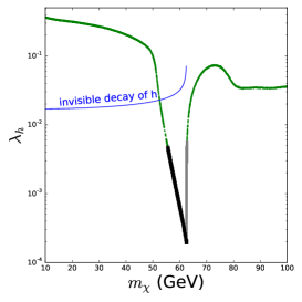
Figure 1: $\lambda_{h}$ consistent with the relic data versus $m_{\chi}$. The dark thick line is allowed by the direct and indirect searches for DM, and the light thick line is excluded by the indirect searches.

IV Dark matter

The two neutral CP-even Higgs can mediate the interactions of DM, $\lambda_{h}v\chi^{2}h/2$ and $\lambda_{H}v\chi^{2}H/2$ with

$$\lambda_{h} \equiv (\lambda_{2}^{\prime}+2\lambda_{5}^{\prime})vs_{\beta}c_{\alpha}-(\lambda_{1}^{\prime}+2\lambda_{4}^{\prime})vc_{\beta}s_{\alpha},$$

$$\lambda_{H} \equiv (\lambda_{2}^{\prime}+2\lambda_{5}^{\prime})vs_{\beta}s_{\alpha}+(\lambda_{1}^{\prime}+2\lambda_{4}^{\prime})vc_{\beta}c_{\alpha}.$$ (21)

We consider a light DM whose freeze-out temperature is much lower than that of EWPT, and thus the effect of EWPT on the current DM relic density can be ignored. We take the new scalars to be much heavier than the DM so that the DM pair-annihilation to these new scalars are kinematically forbidden. In the parameter space chosen previously, the couplings of $H$ to the SM particles can be ignored. Therefore, the DM relic density hardly constrains the $\lambda_{H}$, and $\lambda_{1,2,4,5}^{\prime}$ are allowed to have room enough to produce the pattern of EWPT needed by the EWBG. The annihilation processes with $s$-channel exchange of $h$ are responsible for the relic density. However, for a light $\chi$, the invisible decay $h\to\chi\chi$ is kinematically allowed, and the signal data of the 125 GeV Higgs impose strong upper limits on the $h\chi\chi$ coupling invisible , which is possible to conflict with the requirement of the correct relic density The elastic scattering of $\chi$ on a nucleon receives the contributions of the process with $t$-channel exchange of $h$, which can be strongly constrained by the direct searches experiments of XENON XENON:2018voc . Besides, the indirect searches for DM can impose upper limits on the averaged cross sections of the DM annihilation to $e^{+}e^{-}$, $\mu^{+}\mu^{-}$, $\tau^{+}\tau^{-}$, $u\bar{u}$, $b\bar{b}$, and $WW$ Fermi-LAT:2015att .

After imposing the relevant theoretical and experimental constraints mentioned previously, we show the $\lambda_{h}$ versus $m_{\chi}$ allowed by the invisible decay of the 125 GeV Higgs, the DM relic density, the direct and indirect searches experiments in Fig. 1. From Fig. 1, we find that the DM with a mass of $55$ GeV $\sim 62.5$ GeV is allowed by the joint constraints of the invisible decay of the 125 GeV Higgs, the DM relic density, the direct and indirect searches experiments.

V EWPT and Baryogenesis

We first consider the effective scalar potential at the finite temperature. The neutral elements of $\Phi_{1}$ and $\Phi_{2}$ are shifted by $\frac{h_{1}}{\sqrt{2}}$ and $\frac{h_{2}+ih_{3}}{\sqrt{2}}$. It is plausible to take the imaginary part of the neutral elements of $\Phi_{1}$ to be zero since the effective potential of Eq. (II) only depends on the relative phase of the neutral elements of $\Phi_{1}$ and $\Phi_{2}$ .

The complete effective potential at finite temperature contains the tree level potential, the Coleman-Weinberg term vcw , the finite temperature corrections vloop and the resummed daisy corrections vring1 ; vring2 , which is gauge-dependent vgauge1 ; vgauge2 . Here we consider the high-temperature approximation of effective potential, which keeps only the thermal mass terms in the high-temperature expansion and the tree-level potential. Therefore, the effective potential is gauge invariant, and it does not depend on the renormalization scheme and the resummation scheme. The high-temperature approximation of effective potential is given by

$$V_{eff}(h_{1},h_{2},h_{3},\chi,\eta_{s})=\frac{1}{2}(m_{11}^{2}+\Pi_{h_{1}})h_{1}^{2}+\frac{1}{2}(m_{22}^{2}+\Pi_{h_{2}})(h_{2}^{2}+h_{3}^{2})+\frac{1}{2}(m_{S}^{2}+{m^{\prime}_{S}}^{2}+\Pi_{\chi})\chi^{2}$$

$$+\frac{1}{2}(m_{S}^{2}-{{m^{\prime}_{S}}^{2}}+\Pi_{\eta_{s}})\eta_{s}^{2}+\frac{1}{8}(\lambda_{1}h_{1}^{4}+\lambda_{2}h_{2}^{4}+\lambda_{2}h_{3}^{4})+\frac{1}{4}\lambda_{345}h_{1}^{2}h_{2}^{2}+\frac{1}{4}\bar{\lambda}_{345}h_{1}^{2}h_{3}^{2}$$

$$+\frac{\lambda_{2}}{4}h_{3}^{2}h_{2}^{2}-m_{12}^{2}h_{1}h_{2}-\frac{\mu}{\sqrt{2}}h_{3}\eta_{s}h_{1}+\frac{\lambda^{\prime}_{1}}{4}(\chi^{2}+\eta_{s}^{2})h_{1}^{2}+\frac{\lambda^{\prime}_{2}}{4}(\chi^{2}+\eta_{s}^{2})(h_{2}^{2}+h_{3}^{2})$$

$$+\frac{\lambda^{\prime}_{4}}{2}(\chi^{2}-\eta_{s}^{2})h_{1}^{2}+\frac{\lambda^{\prime}_{5}}{2}(\chi^{2}-\eta_{s}^{2})(h_{3}^{2}+h_{2}^{2})+(\frac{\lambda^{{}^{\prime\prime}}_{1}}{48}+\frac{\lambda^{\prime\prime}_{3}}{16})(\chi^{4}+\eta_{s}^{4})+\frac{1}{8}(\lambda^{\prime\prime}_{3}-\lambda^{\prime\prime}_{1})\chi^{2}\eta_{s}^{2},$$

$$\Pi_{h_{1}}=\left[{9g^{2}\over 2}+{3g^{\prime 2}\over 2}+6\lambda_{1}+4\lambda_{3}+2\lambda_{4}+2\lambda^{\prime}_{1}+6y_{t}^{2}c_{\beta}^{2}\right]{T^{2}\over 24},$$

$$\Pi_{h_{2}}=\left[{9g^{2}\over 2}+{3g^{\prime 2}\over 2}+6\lambda_{2}+4\lambda_{3}+2\lambda_{4}+2\lambda^{\prime}_{2}+{6y_{t}^{2}s_{\beta}^{2}}\right]{T^{2}\over 24},$$

$$\Pi_{h_{3}}=\Pi_{h_{2}},$$

$$\Pi_{\chi}=\left[4\lambda^{\prime}_{1}+4\lambda^{\prime}_{2}+8\lambda^{\prime}_{4}+8\lambda^{\prime}_{5}+2\lambda^{\prime\prime}_{3}\right]{T^{2}\over 24},$$

$$\Pi_{\eta_{s}}=\left[4\lambda^{\prime}_{1}+4\lambda^{\prime}_{2}-8\lambda^{\prime}_{4}-8\lambda^{\prime}_{5}+2\lambda^{\prime\prime}_{3}\right]{T^{2}\over 24},$$ (22)

where $\bar{\lambda}_{345}=\lambda_{3}+\lambda_{4}-\lambda_{5}$, $y_{t}={\sqrt{2}m_{t}\over v}$, and $\Pi_{i}$ denotes the thermal mass terms of the field $i$.

Because baryogenesis is driven by diffusion processes in front of the bubble wall, one needs to compute the $T_{n}$ at which bubble nucleation actually starts. This can be calculated straightforwardly from the nucleation rate per unit volume by bubble-0 ; bubble-1 ; bubble-2 , $\Gamma\approx A(T)e^{-S_{3}/T}$, where $A(T)\sim T^{4}$ is a prefactor and $S_{3}$ is a three-dimensional Euclidian action. The nucleation temperature $T_{n}$ is obtained by $\Gamma/H^{4}$= 1, where $H$ is the Hubble parameter. It is roughly estimated by $\frac{S_{3}(T)}{T}|_{T=T_{n}}=140$. The bubble wall VEV profiles can be determined by the bounce equations of fields.

The WKB approximation method is used to evaluate the CP-violating source terms and chemical potentials transport equations of particle species in the wall frame with a radial coordinate $z$ bg2h-3 ; 0006119 ; 0604159 . A top quark penetrating the bubble wall acquires a complex mass as a function of $z$,

$$m_{t}(z)=\frac{y_{t}}{\sqrt{2}}\sqrt{(c_{\beta}h_{1}(z)+s_{\beta}h_{2}(z))^{2}+s_{\beta}^{2}h^{2}_{3}(z)}~{}e^{i\Theta_{t}(z)},$$

$${\rm with~{}}\Theta_{t}(z)=\varphi_{Z}(z)+\arctan\frac{s_{\beta}h_{3}(z)}{c_{\beta}h_{1}(z)+s_{\beta}h_{2}(z)},$$

$$\partial_{z}\varphi_{Z}(z)=-\frac{h^{2}_{2}(z)+h^{2}_{3}(z)}{h^{2}_{1}(z)+h^{2}_{2}(z)+h^{2}_{3}(z)}\partial_{z}\varphi_{(}z),$$

$$\varphi_{(}z)=\arctan\frac{h_{3}(z)}{h_{2}(z)}.$$ (23)

In our calculation, the imaginary part of the neutral element of $\Phi_{1}$ is taken to be zero. As a result, the nonvanishing $Z_{\mu}$ field induces an additional CP-violating force acting on the top quark, which is removed a local axial transformation of top quark, reintroducing an additional overall phase $\varphi_{Z}(z)$ into $m_{t}$ bg2h-4 .

The transport equations are derived by the complex mass of the top quark, and contains effects of the strong sphaleron process ($\Gamma_{ss}$) bg2h-3 ; 9311367 , W-scattering ($\Gamma_{W}$) bg2h-3 ; 9506477 , the top Yukawa interaction ($\Gamma_{y}$) bg2h-3 ; 9506477 , the top helicity flips ($\Gamma_{M}$) bg2h-3 ; 9506477 , and the Higgs number violation ($\Gamma_{h}$) bg2h-3 ; 9506477 . The transport equations are written as

$$0= 3v_{W}K_{1,t}\left(\partial_{z}\mu_{t,2}\right)+3v_{W}K_{2,t}\left(\partial_{z}m_{t}^{2}\right)\mu_{t,2}+3\left(\partial_{z}u_{t,2}\right)$$

$$-3\Gamma_{y}\left(\mu_{t,2}+\mu_{t^{c},2}+\mu_{h,2}\right)-6\Gamma_{M}\left(\mu_{t,2}+\mu_{t^{c},2}\right)-3\Gamma_{W}\left(\mu_{t,2}-\mu_{b,2}\right)$$

$$-3\Gamma_{ss}\left[\left(1+9K_{1,t}\right)\mu_{t,2}+\left(1+9K_{1,b}\right)\mu_{b,2}+\left(1-9K_{1,t}\right)\mu_{t^{c},2}\right]\,,$$

$$0= 3v_{W}K_{1,t}\left(\partial_{z}\mu_{t^{c},2}\right)+3v_{W}K_{2,t}\left(\partial_{z}m_{t}^{2}\right)\mu_{t^{c},2}+3\left(\partial_{z}u_{t^{c},2}\right)$$

$$-3\Gamma_{y}\left(\mu_{t,2}+\mu_{b,2}+2\mu_{t^{c},2}+2\mu_{h,2}\right)-6\Gamma_{M}\left(\mu_{t,2}+\mu_{t^{c},2}\right)$$

$$-3\Gamma_{ss}\left[\left(1+9K_{1,t}\right)\mu_{t,2}+\left(1+9K_{1,b}\right)\mu_{b,2}+\left(1-9K_{1,t}\right)\mu_{t^{c},2}\right]\,,$$

$$0= 3v_{W}K_{1,b}\left(\partial_{z}\mu_{b,2}\right)+3\left(\partial_{z}u_{b,2}\right)-3\Gamma_{y}\left(\mu_{b,2}+\mu_{t^{c},2}+\mu_{h,2}\right)-3\Gamma_{W}\left(\mu_{b,2}-\mu_{t,2}\right)\,,$$

$$-3\Gamma_{ss}\left[\left(1+9K_{1,t}\right)\mu_{t,2}+(1+9K_{1,b})\mu_{b,2}+(1-9K_{1,t})\mu_{t^{c},2}\right]\,,$$

$$0= 4v_{W}K_{1,h}\left(\partial_{z}\mu_{h,2}\right)+4\left(\partial_{z}u_{h,2}\right)-3\Gamma_{y}\left(\mu_{t,2}+\mu_{b,2}+2\mu_{t^{c},2}+2\mu_{h,2}\right)-4\Gamma_{h}\mu_{h,2}\,,$$

$$S_{t}= -3K_{4,t}\left(\partial_{z}\mu_{t,2}\right)+3v_{W}\tilde{K}_{5,t}\left(\partial_{z}u_{t,2}\right)+3v_{W}\tilde{K}_{6,t}\left(\partial_{z}m_{t}^{2}\right)u_{t,2}+3\Gamma_{t}^{\mathrm{tot}}u_{t,2}\,,$$

$$0= -3K_{4,b}\left(\partial_{z}\mu_{b,2}\right)+3v_{W}\tilde{K}_{5,b}\left(\partial_{z}u_{b,2}\right)+3\Gamma_{b}^{\mathrm{tot}}u_{b,2}\,,$$

$$S_{t}= -3K_{4,t}\left(\partial_{z}\mu_{t^{c},2}\right)+3v_{W}\tilde{K}_{5,t}\left(\partial_{z}u_{t^{c},2}\right)+3v_{W}\tilde{K}_{6,t}\left(\partial_{z}m_{t}^{2}\right)u_{t^{c},2}+3\Gamma_{t}^{\mathrm{tot}}u_{t^{c},2}\,,$$

$$0= -4K_{4,h}\left(\partial_{z}\mu_{h,2}\right)+4v_{W}\tilde{K}_{5,h}\left(\partial_{z}u_{h,2}\right)+4\Gamma_{h}^{\mathrm{tot}}u_{h,2}\,,$$ (24)

The $\mu_{i,2}$ and $u_{i,2}$ are the second-order CP-odd chemical potential and the plasma velocity of the particle $i=t,~{}t^{c},~{}b,~{}h$,. The source term $S_{t}$ is

$$S_{t}=-v_{W}K_{8,t}\partial_{z}\left(m_{t}^{2}\partial_{z}\theta_{t}\right)+v_{W}K_{9,t}\left(\partial_{z}\theta_{t}\right)m_{t}^{2}\left(\partial_{z}m_{t}^{2}\right).$$ (25)

The functions $K_{a,i}$ and $\tilde{K}_{a,i}$ ($a=1-9$) are defined in Ref. 0604159 , and the $\Gamma_{i}^{\mathrm{tot}}$ are the total reaction rate of the particle $i$ bg2h-3 ; 0604159 .

The chemical potential of the left-handed quarks $\mu_{B_{L}}$ is obtained by solving the transport equations. The left-handed quark number is converted into a baryon asymmetry by the weak sphalerons, which is calculated as

$$Y_{B}=\frac{405\Gamma_{ws}}{4\pi^{2}v_{w}g_{*}T_{n}}\int_{0}^{\infty}dz\mu_{B_{L}}(z)f_{sph}(z)\exp\left(-\frac{45\Gamma_{ws}z}{4v_{w}}\right)\,,$$ (26)

where $\Gamma_{ws}\simeq 10^{-6}T_{n}$ is the weak sphaleron rate inside bubble sphaleron-ws and the wall velocity $v_{w}$ is taken as 0.1. The function $f_{sph}(z)=min(1,2.4\frac{T_{n}}{\Gamma_{ws}}e^{-40\xi_{n}(z)/T_{n}})$ with $\xi_{n}(z)=\sqrt{\langle h_{1}\rangle^{2}+\langle h_{2}\rangle^{2}+\langle h_{3}\rangle^{2}}$ is used to smoothly interpolate between the sphaleron rates in the broken and unbroken phases bg2h-4 .

$m_{h}$(GeV)	$m_{H}=m_{H^{\pm}}$(GeV)	$m_{\chi}$(GeV)	$m_{A}$(GeV)	$m_{X}$(GeV)	$m_{12}^{2}$(GeV$)^{2}$
125.0	467.69	55.95	69.80	333.67	2740.09

$t_{\beta}$	$\sin(\beta-\alpha)$	$\sin\theta$	$\lambda^{\prime}_{1}$	$\lambda^{\prime}_{2}$	$\lambda^{\prime}_{4}$	$\lambda^{\prime}_{5}$	$\lambda^{\prime\prime}_{1}=\lambda^{\prime\prime}_{3}$
1.0	1.0	0.324	2.293	1.351	-1.143	-0.675	1.839

Table 1: Input parameters for the BP1, and other parameters are given above.

We focus on the following three-step PTs achieving the spontaneous CP-violation at high temperature and recovering the CP-symmetry. At the first-step PT, the $\eta_{S}$ field firstly acquires a nonzero VEV while $h_{1,2,3}$ still remains zero. The second-step PT is a strongly first-order EWPT converting the origin phase of $h_{1,2,3}$ into an electroweak symmetry broken phase, where $h_{3}$ is required to be nonzero. In order to prevent the electroweak sphalerons to wash out the produced BAU inside the bubbles of broken phase, the PT strength is impose an bound pt-stren , $\frac{\xi_{n}}{T_{n}}>1.0$ in the broken phase. After the third-step PT, the observed vacuum is produced and the CP-symmetry is restored while the BAU is not changed. We employ the package CosmoTransitions to analyze the PTs cosmopt . Some parameter space achieving the three-step PTs are shown in Fig. 2, where we consider the constraints of the vacuum stability, oblique parameter pdg2020 , dark matter observables, and the 125 GeV Higgs signal data, and the data of BAU is not included. From Fig. 2, we find that the three-step PTs satisfying our requirements favor an appropriate value of $\mu$ since the $\mu$ term of Eq. (V) can lead to a close correlation between $\langle h_{3}\rangle$ and $\langle\eta_{s}\rangle$ of the potential minimum. As a result, according to Eq. (9), $m_{A}$ and $m_{X}$ is required to have a large mass splitting.

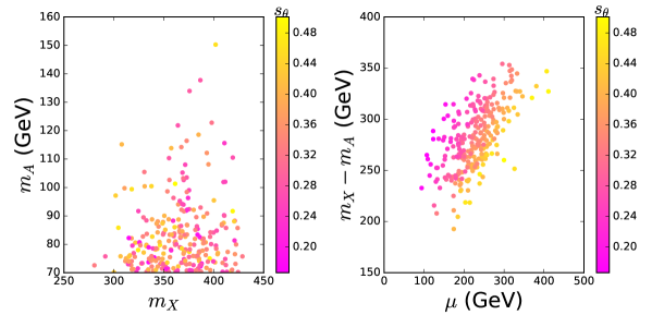
Figure 2: The scattering plots achieving the three-step PTs with the characteristics mentioned in the text, where we take $m_{H}=m_{H^{\pm}}$ and $0.1<s_{\theta}<0.7$.

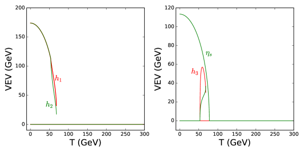
Figure 3: The phase histories of the BP1, where $\langle\chi\rangle$ is always 0.

Figure 4: The radial nucleation bubble wall VEV profiles for the first-order EWPT.

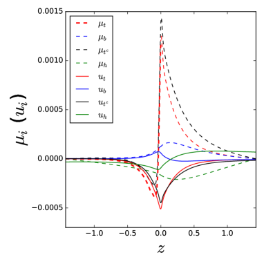
Figure 5: The $\mu_{i}$ and $u_{i}$ from the transport equations as functions of the position of the bubble wall.

We pick out a benchmark point BP1 to discuss the EWPT and baryogenesis detailedly, and the key input parameters are shown in Table 1. The phase histories for the BP1 are shown in Fig. 3. Because the contributions of the thermal mass terms to the effective potential are proportional to $T^{2}$, the minimum of the potential is at the origin at a very high temperature. As the Universe cools, at T=85.38 GeV, a second-order PT takes place during which $\eta_{s}$ acquires a nonzero VEV and the other four fields remain zero. At T=69.65 GeV, a strongly first-order EWPT starts which breaks electroweak symmetry, (0, 0, 0, 0, 73.71) GeV $\to$ (62.42, 34.64, 55.24, 0.0, 37.50) GeV for ($\langle h_{1}\rangle$, $\langle h_{2}\rangle$, $\langle h_{3}\rangle$, $\langle\chi\rangle$, $\langle\eta_{s}\rangle$). The PT strength is 1.30, and the BAU is produced via the EWBG mechanism. At T=52.95 GeV, another second-order PT happens, and then CP-symmetry is recovered. The vacuum evolves along the final phase, and ultimately ends in the observed values at T = 0 GeV. Meanwhile, $\xi_{n}>1$ is always kept so that the BAU is not washed out by the sphaleron processes. The freeze-out temperature of $\chi$ with a mass of 55.95 GeV is around 2.8 GeV, which is much lower than the PT temperatures.

The calculation of BAU depends on the bubble wall profiles, and we use the FindBounce findbounce to obtain the bubble wall VEV profiles for the first-order EWPT of BP1, which is given in Fig. 4. The WKB method of calculating transport equations needs the condition of $L_{W}T_{n}\gg 1$, where $L_{W}$ is the width of bubble wall. The $L_{W}T_{n}$ of BP1 is approximately estimated to be 3.4.

VI Comment on gravitational wave signatures, dark matter, and the LHC signatures

The first-order EWPT needed by the EWBG can produce the gravitational wave. We find that the gravitational wave signatures from the three-step PTs mentioned above can easily exceed the sensitivity curve of the U-DECIGO detector udecigo , such as those of BP1. A full exploration of the parameter space will potentially find promising regions for detectable gravitational wave signal at the BBO bbodecigo . The extra Higgses ($H$, $H^{\pm}$, $A$, $X$) couplings to the SM fermions are significantly suppressed for $\kappa_{u,d,\ell}\to 0$. Therefore, these extra Higgses are dominantly produced at the LHC via the electroweak processes mediated by $Z,W^{\pm}$, and $\gamma$, and the main decay modes include $H\to AZ$, $H^{\pm}\to AW^{\pm}$. The $A$ decay modes depend on specific values of $\kappa_{u,d,\ell}$. For a heavy DM whose freeze-out temperature is higher than the EWPT temperature, the EWPT can give significant effects on the DM relic density. The studies of the LHC signatures and the heavy DM will be carried out in the future.

VII Conclusion

We proposed a complex singlet scalar extension of the 2HDM respecting a discrete dark CP-symmetry. The dark CP-symmetry guarantees $\chi$ to be a DM candidate on one hand and on the other hand allows $\eta_{s}$ to have mixings with the pseudoscalars of the scalar doublet fields, which plays key roles in producing the CP-violation sources needed by the EWBG at high temperature. Imposing relevant theoretical and experimental constraints, we studied the scenario of $m_{\chi}$ around the SM Higgs resonance region, and found that the dark matter relic abundance and the BAU can be simultaneously explained.

References

• (1) P. A. Zyla et al. [Particle Data Group], Review of Particle Physics, PTEP 2020, 083C01 (2020).
• (2) A. D. Sakharov, Violation of CP Invariance, C asymmetry, and baryon asymmetry of the universe, Pisma Zh. Eksp. Teor. Fiz. 5, 32-35 (1967).
• (3) V. A. Kuzmin, V.A. Rubakov, M. E. Shaposhnikov, Phys. Lett. B 155, 36 (1985).
• (4) V. A. Rubakov, M. E. Shaposhnikov, Usp. Fiz. Nauk 166, 493 (1996); Phys. Usp. 39, 461 (1996).
• (5) J. McDonald, Electroweak baryogenesis and dark matter via a gauge singlet scalar, Phys. Lett. B 323, 339 (1994).
• (6) G. C. Branco, D. Delepine, D. Emmanuel-Costa and F.R. Gonzalez, Electroweak baryogenesis in the presence of an isosinglet quark, Phys. Lett. B 442, 229 (1998)
• (7) V. Barger, P. Langacker, M. McCaskey, M. Ramsey-Musolf and G. Shaughnessy, Complex Singlet Extension of the Standard Model, Phys. Rev. D 79, 015018 (2009).
• (8) S. Profumo, M. J. Ramsey-Musolf and G. Shaughnessy, Singlet Higgs phenomenology and the electroweak phase transition, JHEP  08, 010 (2007).
• (9) F. P. Huang, Z. Qian and M. Zhang, Exploring dynamical CP violation induced baryogenesis by gravitational waves and colliders, Phys. Rev. D 98, 015014 (2018).
• (10) A. Beniwal, M. Lewicki, M. White and A. G. Williams, “Gravitational waves and electroweak baryogenesis in a global study of the extended scalar singlet model,” JHEP 02 (2019), 183.
• (11) M. Jiang, L. Bian, W. Huang and J. Shu, Impact of a complex singlet: Electroweak baryogenesis and dark matter, Phys. Rev. D 93, 065032 (2016).
• (12) P. H. Ghorbani, Electroweak Baryogenesis and Dark Matter via a Pseudoscalar vs. Scalar, JHEP 08, 058 (2017)
• (13) W. Chao, CP Violation at the Finite Temperature, Phys. Lett. B 796 (2019), 102-106.
• (14) B. Grzadkowski and D. Huang, Spontaneous $CP$-Violating Electroweak Baryogenesis and Dark Matter from a Complex Singlet Scalar, JHEP 08, 135 (2018)
• (15) K. P. Xie, Lepton-mediated electroweak baryogenesis, gravitational waves and the $4\tau$ final state at the collider, JHEP 02, 090 (2021) [erratum: JHEP 8, 052 (2022)]
• (16) M. Lewicki, M. Merchand and M. Zych, Electroweak bubble wall expansion: gravitational waves and baryogenesis in Standard Model-like thermal plasma, JHEP 02, 017 (2022).
• (17) J. Ellis, M. Lewicki, M. Merchand, J. M. No and M. Zych, The scalar singlet extension of the Standard Model: gravitational waves versus baryogenesis, JHEP 01, 093 (2023).
• (18) C. Idegawa and E. Senaha, “Electron electric dipole moment and electroweak baryogenesis in a complex singlet extension of the Standard Model with degenerate scalars,” [arXiv:2309.09430 [hep-ph]]
• (19) K. Harigaya and I. R. Wang, “First-Order Electroweak Phase Transition and Baryogenesis from a Naturally Light Singlet Scalar,” [arXiv:2207.02867 [hep-ph]].
• (20) N. Turok and J. Zadrozny, Electroweak baryogenesis in the two doublet model, Nucl. Phys. B 358, 471-493 (1991).
• (21) J. M. Cline, K. Kainulainen and A. P. Vischer, Dynamics of two Higgs doublet CP violation and baryogenesis at the electroweak phase transition, Phys. Rev. D 54, 2451-2472 (1996).
• (22) L. Fromme, S. J. Huber and M. Seniuch, Baryogenesis in the two-Higgs doublet model, JHEP  11, 038 (2006).
• (23) S. Kanemura, Y. Okada and E. Senaha, “Electroweak baryogenesis and quantum corrections to the triple Higgs boson coupling,” Phys. Lett. B 606 (2005), 361-366.
• (24) P. Basler, M. Mühlleitner and J. Wittbrodt, “The CP-Violating 2HDM in Light of a Strong First Order Electroweak Phase Transition and Implications for Higgs Pair Production,” JHEP 03 (2018), 061.
• (25) T. Abe, J. Hisano, T. Kitahara and K. Tobioka, “Gauge invariant Barr-Zee type contributions to fermionic EDMs in the two-Higgs doublet models,” JHEP 01 (2014), 106; [erratum: JHEP 04 (2016), 161].
• (26) S. Tulin and P. Winslow, Anomalous B meson mixing and baryogenesis, Phys. Rev. D 84, 034013 (2011).
• (27) J. M. Cline, K. Kainulainen and M. Trott, Electroweak Baryogenesis in Two Higgs Doublet Models and B meson anomalies, JHEP  11, 089 (2011).
• (28) T. Liu, M. J. Ramsey-Musolf and J. Shu, Electroweak Beautygenesis: From $b\to s$ CP-violation to the Cosmic Baryon Asymmetry, Phys. Rev. Lett. 108, 221301 (2012)
• (29) M. Ahmadvand, Baryogenesis within the two-Higgs-doublet model in the Electroweak scale, Int. J. Mod. Phys. A 29, 1450090 (2014).
• (30) C. W. Chiang, K. Fuyuto and E. Senaha, Electroweak Baryogenesis with Lepton Flavor Violation, Phys. Lett. B 762, 315 (2016).
• (31) H. K. Guo, Y. Y. Li, T. Liu, M. Ramsey-Musolf and J. Shu, Lepton-Flavored Electroweak Baryogenesis, Phys. Rev. D 96, 115034 (2017).
• (32) T. Modak and E. Senaha, Electroweak baryogenesis via bottom transport, Phys. Rev. D 99, 115022 (2019).
• (33) P. Basler, M. Mühlleitner and J. Müller, BSMPT v2 a tool for the electroweak phase transition and the baryon asymmetry of the universe in extended Higgs Sectors, Comput. Phys. Commun. 269, 108124 (2021)
• (34) R. Zhou, L. Bian, Gravitational wave and electroweak baryogenesis with two Higgs doublet models, Phys. Lett. B 829, 137105 (2022).
• (35) P. Basler, M. Mühlleitner and J. Müller, Electroweak Baryogenesis in the CP-Violating Two-Higgs Doublet Model, Eur. Phys. J. C 83, 57 (2023).
• (36) K. Enomoto, S. Kanemura, Y. Mura, Electroweak baryogenesis in aligned two Higgs doublet models, JHEP  01, 104 (2022).
• (37) K. Enomoto, S. Kanemura, Y. Mura, New benchmark scenarios of electroweak baryogenesis in aligned two Higgs double models, JHEP  09, 121 (2022).
• (38) D. Gonçalves, A. Kaladharan and Y. Wu, “Gravitational waves, bubble profile, and baryon asymmetry in the complex 2HDM, Phys. Rev. D 108 (2023), 075010
• (39) ACME collaboration, J. Baron et al., Order of Magnitude Smaller Limit on the Electric Dipole Moment of the Electron, Science 343, 269 (2014)
• (40) L. Bian, T. Liu, J. Shu, Cancellations Between Two-Loop Contributions to the Electron Electric Dipole Moment with a CP-Violating Higgs Sector, Phys. Rev. Lett. 115, 021801 (2015).
• (41) K. Fuyuto, W. S. Hou and E. Senaha, “Electroweak baryogenesis driven by extra top Yukawa couplings,” Phys. Lett. B 776 (2018), 402-406.
• (42) T. Modak and E. Senaha, “Electroweak baryogenesis via bottom transport,” Phys. Rev. D 99 (2019), 115022.
• (43) K. Fuyuto, W. S. Hou and E. Senaha, “Cancellation mechanism for the electron electric dipole moment connected with the baryon asymmetry of the Universe,” Phys. Rev. D 101 (2020), 011901.
• (44) T. Modak and E. Senaha, “Probing Electroweak Baryogenesis induced by extra bottom Yukawa coupling via EDMs and collider signatures,” JHEP 11 (2020), 025.
• (45) S. Kanemura, M. Kubota and K. Yagyu, Aligned CP-violating Higgs sector canceling the electric dipole moment, JHEP  08, 026 (2020).
• (46) S. J. Huber, K. Mimasu and J. M. No, Baryogenesis from spontaneous CP violation in the early Universe, Phys. Rev. D 107, (2023) 075042.
• (47) S. Liu and L. Wang, “Spontaneous CP violation electroweak baryogenesis and gravitational wave through multistep phase transitions,” Phys. Rev. D 107 (2023), 115008.
• (48) A. Pich, P. Tuzon, Yukawa Alignment in the Two-Higgs-Doublet Model, Phys. Rev. D 80, (2009) 091702.
• (49) L. Wang and X. F. Han, Status of the aligned two-Higgs-doublet model confronted with the Higgs data, JHEP 04, 128 (2014).
• (50) K. Kannike, “Vacuum Stability Conditions From Copositivity Criteria,” Eur. Phys. J. C 72 (2012), 2093 arXiv:1205.3781.
• (51) J. Dutta, J. Lahiri, C. Li, G. Moortgat-Pick, S. F. Tabira and J. A. Ziegler, “Dark Matter Phenomenology in 2HDMS in light of the 95 GeV excess,” arXiv:2308.05653.
• (52) W. Porod, “SPheno, a program for calculating supersymmetric spectra, SUSY particle decays and SUSY particle production at e+ e- colliders, Comput. Phys. Commun. 153 (2003), 275-315 arXiv:hep-ph/0301101.
• (53) F. Staub, “SARAH 4 : A tool for (not only SUSY) model builders,” Comput. Phys. Commun. 185 (2014), 1773-1790 arXiv:1309.7223.
• (54) H.-J. He, N. Polonsky, S. Su, Extra families, Higgs spectrum and oblique corrections, Phys. Rev. D 64, (2001) 053004.
• (55) H. E. Haber, D. ONeil, Basis-independent methods for the two-Higgs-doublet model. III. The CP-conserving limit, custodial symmetry, and the oblique parameters S, T, U, Phys. Rev. D 83, (2011) 055017. .
• (56) ATLAS Collaboration, M. Aaboud et al., Search for an invisibly decaying Higgs boson or dark matter candidates produced in association with a Z boson in pp collisions at $\sqrt{s}$ = 13 TeV with the ATLAS detector, Phys. Lett. B 776, (2018) 318-337.
• (57) Planck Collaboration, Planck 2015 results. XXVII. The Second Planck Catalogue of Sunyaev-Zeldovich Sources, Astron. Astrophys. 27, 594 (2016).
• (58) E. Aprile et al. [XENON], “Dark Matter Search Results from a One Ton-Year Exposure of XENON1T,” Phys. Rev. Lett. 121 (2018), 111302.
• (59) M. Ackermann et al. [Fermi-LAT], “Searching for Dark Matter Annihilation from Milky Way Dwarf Spheroidal Galaxies with Six Years of Fermi Large Area Telescope Data,” Phys. Rev. Lett. 115, (2015) 231301.
• (60) S. R. Coleman and E. J. Weinberg, Radiative Corrections as the Origin of Spontaneous Symmetry Breaking, Phys. Rev. D 7, 1888 (1973).
• (61) L. Dolan and R. Jackiw, Symmetry Behavior at Finite Temperature, Phys. Rev. D 9, 3320 (1974).
• (62) P. B. Arnold and O. Espinosa, The Effective potential and first order phase transitions:Beyond leading-order, Phys. Rev. D 47, 3546 (1993) [Erratum: Phys. Rev. D 50, 6662 (1994)].
• (63) R. R. Parwani, Resummation in a hot scalar field theory, Phys. Rev. D 45, 4695 (1992).
• (64) R. Jackiw, Functional evaluation of the effective potential, Phys. Rev. D 9, 1686 (1974).
• (65) H. H. Patel and M. J. Ramsey-Musolf, Baryon Washout, Electroweak Phase Transition, and Perturbation Theory, JHEP  07, 029 (2011).
• (66) I. Affleck, Quantum Statistical Metastability, Phys. Rev. Lett. 46, 388 (1981).
• (67) A. D. Linde, Decay of the False Vacuum at Finite Temperature, Nucl. Phys. B 216, 421 (1983) [Erratum: Nucl. Phys. B 223, 544 (1983)].
• (68) A. D. Linde, Fate of the False Vacuum at Finite Temperature: Theory and Applications, Phys. Lett. B 100, 37-40 (1981).
• (69) J. M. Cline, M. Joyce and K. Kainulainen, Supersymmetric electroweak baryogenesis, JHEP  07, 018 (2000).
• (70) L. Fromme and S. J. Huber, Top transport in electroweak baryogenesis, JHEP  03, 049 (2007).
• (71) G. F. Giudice and M. E. Shaposhnikov, Strong sphalerons and electroweak baryogenesis, Phys. Lett. B 326, 118-124 (1994).
• (72) P. Huet and A. E. Nelson, Phys. Rev. D 53, 4578 (1996).
• (73) G. D. Moore, Sphaleron rate in the symmetric electroweak phase, Phys. Rev. D 62, 085011 (2000).
• (74) G. D. Moore, Measuring the broken phase sphaleron rate nonperturbatively, Phys. Rev. D 59, 014503 (1999).
• (75) C. L. Wainwright, CosmoTransitions: Computing Cosmological Phase Transition Temperatures and Bubble Profiles with Multiple Fields, Computl. Phys. Commun. 183, 2006-2013 (2012).
• (76) V. Guada, M. Nemevšek and M. Pintar, FindBounce: Package for multi-field bounce actions, Comput. Phys. Commun. 256, 107480 (2020)
• (77) J. R. Espinosa, B. Gripaios, T. Konstandin, and F. Riva, Electroweak Baryogenesis in Non-minimal Composite Higgs Models, JCAP 01, 012 (2012).
• (78) J. McDonald, Phys. Lett. B 323, 339 (1994).
• (79) H. Kudoh, A. Taruya, T. Hiramatsu, and Y. Himemoto, Detecting a gravitational-wave background with next-generation space interferometers, Phys. Rev. D 73, 064006 (2006).
• (80) K. Yagi and N. Seto, Detector configuration of DECIGO/BBO and identification of cosmological neutron-star binaries, Phys. Rev. D 83, 044011 (2011).