Mesh Neural Cellular Automata

Abstract

Modeling and synthesizing textures are essential for enhancing the realism of virtual environments. Methods that directly synthesize textures in 3D offer distinct advantages to the UV-mapping-based methods as they can create seamless textures and align more closely with the ways textures form in nature. We propose Mesh Neural Cellular Automata (MeshNCA), a method for directly synthesizing dynamic textures on 3D meshes without requiring any UV maps. MeshNCA is a generalized type of cellular automata that can operate on a set of cells arranged on a non-grid structure such as vertices of a 3D mesh. While only being trained on an Icosphere mesh, MeshNCA shows remarkable generalization and can synthesize textures on any mesh in real time after the training. Additionally, it accommodates multi-modal supervision and can be trained using different targets such as images, text prompts, and motion vector fields. Moreover, we conceptualize a way of grafting trained MeshNCA instances, enabling texture interpolation. Our MeshNCA model enables real-time 3D texture synthesis on meshes and allows several user interactions including texture density/orientation control, a grafting brush, and motion speed/direction control. Finally, we implement the forward pass of our MeshNCA model using the WebGL shading language and showcase our trained models in an online interactive demo which is accessible on personal computers and smartphones. Our demo and the high resolution version of this PDF are available at https://meshnca.github.io/.

Figure 1: Our Mesh Neural Cellular Automata (MeshNCA) synthesizes 3D surface textures in real time and exhibits various intriguing test-time properties that facilitate user interaction. Train: MeshNCA is only trained on an icosphere guided by the target appearance. Test-time Generalization: (a) MeshNCA generalizes to unseen mesh during test time; (b) By simply subdividing the mesh, we can control the texture density in real time. Test-time Controls: Users can readily control the behavior of MeshNCA at test time, including (c) texture orientation, (d) texture grafting, (e) self-regeneration, and (f) motion. See our real-time interactive demo at https://meshnca.github.io/.

1 Introduction

The appearance of objects surrounding us is primarily determined by their textures. Modeling and synthesizing textures are key components for enhancing the realism and visual appeal of virtual environments. By enriching the surface-level details of 3D models, textures add depth, complexity, and authenticity to the digital worlds we create.

Various methods have been developed to synthesize textures for 3D objects, most of which fall into two main categories. 1) Methods that synthesize textures directly within a 3D space, and 2) methods that synthesize textures in a 2D domain which are then mapped onto a 3D surface via UV mapping. While UV-mapping-based methods are the most common approach due to their simplicity and compatibility with existing graphics pipelines [17, 18, 13, 39, 21], they come with an inherent limitation: the process of creating accurate UV maps for intricate 3D objects often leads to visible artifacts such as overlapping regions, distortions, visible seams.

In this paper, we focus on the methods that directly synthesize textures in 3D. These methods offer a set of inherent advantages. Primarily, they can naturally produce seamless textures due to their independence from UV maps. Moreover, they tend to align more closely with the natural texture formation processes, including phenomena like growth, erosion, and deposition [24], all of which occur in 3D space. We classify these methods into three groups: Solid Textures, Surface Textures, and Cellular Automata (CA).

Solid Texture synthesis methods assign colors to the points inside a 3D volume. Although this approach is suitable for modeling textures carved out of a solid block, such as wood or marble, it is not apt for modeling texture-related processes that take place on the surface of an object, such as motion or erosion. Instead, Surface Texture synthesis approaches directly assign a color to each point on the surface of an object. While these methods can be aware of the underlying 3D surface, they do not allow any user interaction to edit the synthesized texture and require retraining for each 3D mesh separately. Lastly, Cellular Automata models utilize local update rules to generate textures, mirroring the dynamic behaviors seen in natural systems such as Reaction-Diffusion [44]. These methods offer many test-time controls and allow the users to interact with the synthesized texture. However, they require manual design for each texture and cannot be trained to synthesize a target texture.

In this paper, we focus on Cellular-Automata-based 3D texture modeling since this approach offers the most user interaction, which is of paramount importance for design, art, and creative applications. We build upon Neural Cellular Automata (NCA), a differentiable counterpart of conventional CA [29, 31]. NCA models are parameterized by very small neural networks and have proven to be effective for texture synthesis due to various advantages they possess, such as parameter efficiency [26], inherent parallelizability [31, 33], a capability to operate at arbitrary resolutions [31], real-time user interactivity [31], and their adeptness at texture motion control [33].

One major limitation of NCA models is that the cells should be aligned in a regular grid like the pixels of an image. We generalize NCAs beyond the regular grid structure and allow them to operate on an arbitrary arrangement of cells given by a mesh. We call our model Mesh Neural Cellular Automata (MeshNCA). MeshNCA enables real-time and interactive texture synthesis on 3D meshes while entailing all the remarkable properties of 2D NCAs. Figure 1 displays the test-time properties of our MeshNCA model including: generalization to unseen meshes, texture density control using mesh subdivision, texture orientation control, self-organization, and texture motion control. Our development ensures minimal computational overhead, preserving the efficiency inherent to the 2D NCA model. This optimization facilitates the smooth operation of MeshNCA even on edge devices. Additionally, we propose a way of grafting two NCA models in test time to produce smooth transitions from one texture to another.

MeshNCA works by replacing the 2D convolution kernels of the NCA model with a more general message-passing scheme based on spherical harmonics. Mesh vertices constitute the cells in our model and the edges of the mesh define the neighborhood for each cell. We train our model to synthesize a target exemplar texture, described either by an image or a text prompt. While MeshNCA is only trained on an Icosphere mesh, Remarkably, it can generalize to any mesh in test-time, as it only relies on local interactions between the cells. Moreover, by simply subdividing the input mesh in test-time, our model can produce a texture at different levels of density. Our contributions are summarized as follows:

1. We introduce MeshNCA, a novel model for real-time and interactive texture synthesis on 3D meshes. Notably, our model possesses remarkable generalization capabilities along with diverse test-time properties.

2. MeshNCA can be trained under either image or text guidance, facilitating multimodal texture synthesis.

3. We perform 3D dynamic texture synthesis by guiding the motion of the synthesized 3D texture through projected 2D motion supervision. Intriguingly, MeshNCA can seamlessly adapt and synthesize the correct motion patterns on unseen meshes.

4. We propose MeshNCA grafting, where two MeshNCA models cooperate to synthesize brand-new hybrid textures during test time.

5. We implement the forward pass of our MeshNCA model using the WebGL shading language and showcase various user interactions and numerous test-time properties of MeshNCA. Our demo runs in real time on low-end edge devices, proving the efficiency of MeshNCA, and is available at https://meshnca.github.io/.

2 Related Works

In the following section, we discuss existing 3D texture synthesis methods. For comparison, Table 1 summarizes the strengths (✓) and shortcomings (✗) of these methods.

Type	Method	#$\mathbf{\theta}$	A	B	C	D	E	F	G	H
Solid Textures	[35, 34]	$10^{1}$	✗	✓	✗	✗	✓	✓	✓	✗
	Kopf et al. [20]	$10^{7}$	✓	✓	✓	✗	✓	✗	✓	✗
	[16, 36, 14]	$10^{5}$	✓	✓	✓	✗	✓	✓	✓	✗
	Oechsle et al. [32]	$10^{8}$	✗	✓	✓	✗	✓†	✓	✗	✗
	Michel et al. [25]	$10^{7}$	✓	✗	✓	✗	✗	✓	✗	✗
Surface Textures	[46, 47, 48, 50]	$10^{5}$	✓	✗	✓	✗	✗	✗	✗	✗
	Han et al. [15]	$10^{5}$	✓	✗	✓	✓	✗	✗	✗	✗
	[40, 3]	$10^{8}$	✗	✗	✓	✗	✓†	✓	✗	✗
Cellular Automata	Turk et al. [45]	$10^{1}$	✗	✗	✗	✓‡	✓	✓	✓	✗
	Fleischer et al. [7]	$10^{2}$	✗	✗	✗	✓	✗	✓	✗	✗
	Gobron et al. [11]	$10^{1}$	✗	✓	✗	✓‡	✓	✓	✗	✗
	Mordvintsev et al. [28]	$10^{4}$	✓	✗	✓	✓‡	✓	✓	✗	✗
	MeshNCA (Ours)	$10^{4}$	✓	✗	✓	✓	✓	✓	✓	✓

Table 1: Comparison of 3D texture synthesis methods. (#$\mathbf{\theta}$) Shows the number of parameters required to synthesize new textures. (A) Can synthesize a diverse set of textures (B) Does not need high poly meshes (C) Does not require manual parameter tuning (can be trained) (D) Can produce dynamic textures on 3D meshes (E) Does not need re-training for a new mesh (F) Can synthesize new texture instances in real-time (G) Allows re-orienting the texture on the 3D mesh (H) Allows texture grafting. ✓^† Cannot generalized beyond the mesh categories in the training dataset. ✓^‡ The motion is random and cannot be controlled.

2.1 Solid Texture Synthesis

The seminal work by Peachey [34] and Perlin [35] in 1985, introduced the concept of Solid Textures and the idea of using a space function to map a 3D coordinate to a color. Solid textures eliminate the need to design UV maps for texturing a mesh. However, their proposed approach can not produce a diverse set of textures and requires tedious manual design processes to obtain a specific texture. To enable synthesizing a more diverse set of textures, Kopf et al. [20] propose an optimization-based method that creates an explicit solid texture volume from a 2D exemplar texture.

Extending the idea of solid texturing into the deep learning era, Henzler et al. [16] leverage Multi Layered Perceptron (MLP) to model the coordinate-to-color mapping function. Following the work of Perlin et al. [35], the input coordinates to the MLP are first transformed into noise at multiple frequency levels. Portenier et al. [36] propose to inject the noise into the hidden layers of MLP. Gutierrez et al. [14] use a 3D convolutional neural network to transform the input noise into a solid texture volume. For training, all of these use a form of Gram loss [10] and evaluate it on 2D slices of the synthesized solid texture.

Instead of slice-based training, Michel et al. [25] utilize a differentiable renderer to directly texture a given mesh. They apply positional encoding on the vertex coordinates and use an MLP to output color and displacement values for each vertex. Improvements have been made towards dynamically incorporating the text guidance information [23] or fitting to more vertex attributes [22]. Oechsle et al. [32] represent solid textures using a residual MLP which is conditioned on the shape code of the target object and the appearance code of the intended texture. While Solid Texturing methods can craft high-fidelity textures on 3D meshes, they are fundamentally incapable of resembling texture-related processes that happen on the surface of objects such as motion.

2.2 Surface Texture Synthesis

Synthesizing surface texture corresponds to assigning a color for each point on the surface. Early approaches rely on intricate designs of neighborhoods on 3D surfaces and determining the vertex color based on the Markov Random Field (MRF) model for textures [6, 8]. The neighborhood construction scheme includes surface sweeping [46], template matching [47], and neighborhood mapping from 2D to 3D [48]. After obtaining the neighborhood for a vertex, the algorithm searches for the best matching patch from the 2D exemplar texture and assigns the central pixel’s color to the corresponding vertex. Han et al. utilize discrete optimization techniques to improve the synthesis performance [15]. Moreover, additional user-provided inputs, such as texton masks [50] or vector fields [15], can be incorporated into the training to synthesize progressive-variant textures [50] and dynamic textures on the surface [15], respectively. These methods allow modeling surface-related texture processes such as motion. Nevertheless, they require a from-scratch optimization for a new mesh and do not allow real-time user interaction.

Recently, deep learning models have significantly contributed to surface texture synthesis. Siddiqui et al. [40] propose to use a GAN training scheme in which the generator predicts target textures based on surface-feature-conditioned latent code. Building on this, Bokhovkin et al. [3] incorporate an MLP to achieve more detailed face textures. In a different approach, Richardson et al. [38] and Chen et al. [4] develop diffusion-model-guided 2D-to-3D surface texture synthesis, utilizing a partitioned view representation. These methods excel in producing object-aware semantic textures. However, these strategies either necessitate computationally demanding models or need retraining for new meshes. Furthermore, some methods’ dependency on predefined UV mapping restricts their utility for meshes in the wild [25, 21].

2.3 Cellular Automata For Texture Synthesis

Cellular Automata (CA) [30] models have three main components: cell state, neighborhood, and update rule. The cell state stores all the information of a cell such as color. The update rule is based on the state of the cell and its neighboring cells and defines how the cell states change over time. Inspired by Turing’s seminal work [44] proposing the Reaction-Diffusion (RD) model , Turk et al. [45] extend the reaction-diffusion simulation to arbitrary surfaces using Voronoi region-based neighborhood definition. Gobron et al. [11] extend 2D cellular automata [30] to the 3D domain by discretizing mesh polygons with regular grids and subsequently performing 2D CA updates for each polygon. Fleischer et al. [7] devise an elaborate cell simulation, in which solving a set of PDEs defined on cell attributes yields various textures. These CA-based models have the potential to generate 3D textures in real time and can generalize to a new mesh without retraining. However, all of these models rely on a manually crafted set of rules which makes them incapable of synthesizing a diverse set of textures.

To address this issue, Neural Cellular Automata [29] is proposed as a trainable counterpart of the traditional CA and reaction-diffusion systems. Niklasson et al. [31, 26] train NCA models to synthesize 2D textures. Mordvinstev et al. [28] resort to the Laplacian operator which allows them to transpose a 2D reaction-diffusion model onto the surface of 3D meshes. However, due to the isotropic nature of the Laplacian operator, their model is unaware of directional information and thus has limited capability of texture learning. Our proposed model, MeshNCA, leverages non-parametric spherical-harmonics-based filters to incorporate directional information for all cells while preserving the purely local communication scheme. Hence, MeshNCA acts as a natural extension of the 2D NCA models into the 3D domain, while retaining all its remarkable properties such as efficiency, robustness, and controllability.

3 Method

In the following sections, we will begin with an examination of NCA models and their limitations and then explain the details of our MeshNCA model which serves as a more generalized version of the vanilla NCA. Finally, we propose a scheme for grafting two NCA models to create interactive texture interpolation.

3.1 Preliminaries

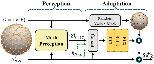
Figure 2: A single update step of MeshNCA. The underlying graph topology of the mesh is given by $G$. At each time step $t$, the cell states $\mathbf{S}^{t}_{N\times C}$ first pass through the Mesh Perception where each cell collects information from its neighborhood anisotropically. The obtained perception tensor $\mathbf{Z}^{t}_{N\times 4C}$ is concatenated to the cell states and an optional per-cell conditional vector $h_{N\times d}$. Each cell then updates its cell state via the same Adaptation rule, parametrized by a two-layer MLP. The MLP outputs the residual update for cell adaptation and all cells perform a stochastic update by multiplying a random vertex mask. Consequently, the cell states at time step $t+\Delta t$ are determined. We set $\Delta t=1$ in our experiments.

Cell states, Neighborhood Function, and Local Update Rule are the core components of any Cellular Automata model. The cell states at time $t$ is represented by $\mathbf{S}^{t}\in\mathbb{R}^{N\times C}$, where $N$ is the total number of cells and $C$ is the dimensionality of a single cell state. A neighborhood function $\mathcal{N}$ represents the neighboring relations between the cells such that $\mathcal{N}(i)=\{j\;|\;j\textup{ is a neighbor of }i\}$, where $i,j$ are cell indices. All the cells in a CA model follow the same local update rule. This update rule determines the next state of each cell based on the cell’s state and its neighboring cell states.

Neural Cellular Automata models are a subset of CA models in which the update rule is parameterized by a neural network. We decompose the local update rule in NCA models into two parts: Perception stage and Adaptation stage. In the Perception stage each cell receives information from its local neighborhood, thereby forming the perception vector $Z\in\mathbb{R}^{N\times C^{\prime}}$. This newly gathered information subsequently directs the updating of the cell’s state in the Adaptation stage. Notice that the perception stage is the only part of the update rule that allows the cells to receive information from their neighboring cells.

During the perception stage each cell gathers information from its neighboring cells. The existing NCA models use the Moore neighborhood and operate on a regular grid of cells where the state can be represented as $\mathbf{S}^{t}\in\mathbb{R}^{H\times W\times C}$. They utilize frozen convolution kernels including Sobel and Laplacian to perform the perception operation [29, 31, 26, 33]. Using Sobel and Laplacian kernels offers the advantage of enabling interactive directional controls in testing time [31, 33]. However, this approach constrains the applicability of existing NCA models to grid-like, regular cell structures like pixel images, preventing their use with more flexible cell structures such as 3D meshes.

Our MeshNCA model extends the vanilla NCA, enabling it to work with arbitrarily positioned sets of cells and removing the need for a grid cell structure. We model the perception stage of MeshNCA using the message-passing scheme in Graph Neural networks [49, 12] and generalize the convolution filters of vanilla NCA to any arbitrary cell structure by utilizing Spherical Harmonics. In the following section, we elaborate on the MeshNCA architecture.

3.2 MeshNCA Architecture

We use graphs to represent the arrangement of the cells in our model. Given a mesh, we construct a graph $\mathbf{G}=(V,E)$ where $V\in\mathbb{R}^{N\times 3}$ denotes the vertices of the mesh and their 3D positions and $E$ denotes the edges of the mesh. The nodes of this graph represent the cells and the edges of the graph determine the neighborhood relations between the cells. In this work, we use undirected edges to have a symmetric neighborhood relationship between the cells. MeshNCA interprets each vertex of the mesh as a cell and updates the cell states over time, starting from a constant zero tensor $\mathbf{S}^{0}$ as the initial state. Figure 2 illustrates one step of the MeshNCA update rule. We decompose the update rule into two main stages, Perception, and Adaptation, which will be further explained in the following sections.

3.2.1 Perception Stage

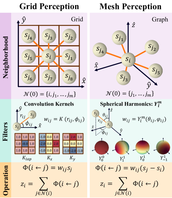
Figure 3: A comparison between regular Grid Perception and our Mesh Perception on three terms.Neighborhood: In grid perception, the neighbor cells of the center node have fixed relative direction and distance, while the neighborhoods in mesh perception can have arbitrary positions. Filters: The convolution filters in grid perception can be rewritten as a function of the distance and direction between the center node and its neighbor. Extending this idea, we use spherical harmonics as the basis of our mesh perception filter as they provide a continuous response to the input direction. Operation: Both perception methods share similar information-gathering operations to form the perception vector $z$.

Figure 3 shows an overview of our Mesh Perception stage. We use the message-passing scheme of Graph Neural networks [49] as the basis of our Mesh Perception. During the message-passing, each cell $i$ receives a message $\Phi(i\leftarrow j)$ from the cell $j$. The perception vector for each cell is simply the summation of all the messages received by that cell:

$$z_{i}=\sum_{j\in\mathcal{N}(i)}\Phi(i\leftarrow j)$$ (1)

The main idea behind our Mesh Perception is to generalize the 2D convolution kernels of the vanilla NCA model to non-grid structures such as meshes by reformulating the convolution operation using a graph-based message-passing scheme. Our key insight is that any 2D convolution filter is a discrete lookup table that can be realized using a continuous function $filter(\phi_{ij},r_{ij})$ which maps the distance $r_{ij}$ and the polar angle $\phi_{ij}$ between two pixels $i$ and $j$ to a coefficient $w_{ij}$ as shown in Figure 3. The message that the center cell $i$ receives from its neighbor cell $j$ is then defined as $\Phi(i\leftarrow j)=w_{ij}s_{j}$ where $s_{j}$ is the state of the neighbor cell $j$. The vanilla NCA architecture uses 3 different convolution filters in the perception stage including two Sobel filter $K_{x},K_{y}$ and one Laplacian filter $K_{lap}$. For example, the weights of the Sobel filter $w_{ij}=K_{x}(\phi_{ij},r_{ij})$ can be realized using the following function:

$$K_{x}(\phi_{ij},r_{ij})=\left\{\begin{matrix}0&\textup{if}\;r_{ij}=0\\ 2\;\textup{sgn}(\cos\phi_{ij})\cos^{2}(\phi_{ij})&\textup{otherwise}\end{matrix}\right.$$

where sgn is the Sign function.

Interpreting convolution filters as functions facilitates the extension to non-grid structures such as meshes. For two arbitrarily located cells $i$ and $j$ in 3D space, a filter function can be written as $f(r_{ij},\theta_{ij},\phi_{ij})$ where $[r_{ij},\theta_{ij},\phi_{ij}]$ are the spherical coordinates of the vector connecting the cell $i$ to the cell $j$. We find that removing the dependence on the distance $r_{ij}$ is not harmful to the expressivity of our model and for texture synthesis. Therefore, we only consider the functions of the form $f(\theta_{ij},\phi_{ij})$, and choose Spherical Harmonics $Y^{m}_{l}(\theta,\phi)$ as the basis of our Mesh Perception filters as shown in Figure 3. We use the first-order spherical harmonics, $l\leq 1$, leading to four basis functions as our filters. For each filter $Y^{m}_{l}$, we evaluate the message coefficient $w_{ij}=Y^{m}_{l}(\theta_{ij},\phi_{ij})$ and use the following equation

$$\Phi(i\leftarrow j)=w_{ij}(s_{j}-s_{i})$$ (2)

to evaluate the message passed from neighbor cell $j$ to the center cell $i$. With our proposed message passing scheme introduced in Equation 2, the first four spherical harmonics become analogous to the Laplacian and Sobel filters, where $Y^{0}_{0}$ corresponds to the Laplacian filter $K_{lap}$ and $Y^{1}_{1},Y^{1}_{0},Y^{1}_{-1}$ correspond to the Sobel filters $K_{x},K_{z},K_{y}$, respectively. Notice that our mesh perception is completely non-parametric and is not optimized during the training.

As shown in Figure 2, the output of the perception stage is $Z^{t}_{N\times 4C}$, where $z^{t}_{i}$ is the perception vector of the cell with index $i$ at time step $t$. The $4\textup{x}$ expansion in the number of channels comes from the fact that we use the first four spherical harmonics bases in our perception filters. We refer the reader to section 7 for an ablation study on the degree of the spherical harmonics used in our model.

3.2.2 Adaptation Stage

In the Adaptation stage each cell $i$ independently updates its own state based on the information available to it. This information constitutes $z_{i}^{t}\in\mathbb{R}^{4C}$, $s_{i}^{t}\in\mathbb{R}^{C}$ and $h_{i}\in\mathbb{R}^{d}$ where $z_{i}^{t},s_{i}^{t}$ are the perception vector and the state of the cell at the current step. The vector $h_{i}$ stores the optional per-cell conditional information. We concatenate $z_{i}^{t},s_{i}^{t}$, and $h_{i}$ in the channel dimension and pass the resulting $5C+d$ dimensional vector to Multi-Layered-Perceptron (MLP) with two layers and a ReLU activation function. The output of the MLP is then masked by a random variable $M$ having Bernoulli distribution with $p=0.5$ and added to the current state as shown in the following equation:

$$s^{t+1}_{i}=\left\{\begin{matrix}s^{t}_{i}&M=0\\ s^{t}_{i}+\textup{MLP}(s^{t}_{i},z^{t}_{i},h_{i})&M=1\end{matrix}\right.$$ (3)

The stochastic random vertex masking fosters asynchronicity in the update rule and enables the NCA to generate new textures over time. Notice that all of the operations in the adaptation are vertex-wise and can be executed in parallel for all the cells, thus allowing for an efficient implementation.

3.3 Grafting

We introduce a useful property of NCA we term ”grafting”, named after the practice of physically joining the tissues of different plants, within the same species. Grafting allows spatially interpolating between two different MeshNCA textures on the same mesh. It requires both a particular method of test-time interpolation and a particular training scheme. In the following sections, we will elaborate on the concept of grafting and texture interpolation, and propose our method for test-time grafting of MeshNCA instances. The training scheme for acquiring graftable MeshNCA instances is detailed in Section 4.4.

3.3.1 Challenges of Texture Interpolation

Interpolating synthesized textures is a non-trivial problem involving matching both microscopic and macroscopic features in a natural way. We invite readers to consider the, perhaps non-intuitive, complexity of this task. Suppose you have a textured brick wall, which has to transition into another brick wall that is textured with entirely different masonry. In the physical world, this would naturally involve a form of coordination by the stonemason between the two types of bricks - the bricks have to physically interleave each other without gaps. If you simply have a procedurally generated brick texture, however, having two different such procedural algorithms to interleave correctly is a highly non-trivial task. Furthermore, implementing such an interpolation which produces correct results for any two pairs of textures is even harder. One naive way of approaching this problem would be to explicitly align a terminating edge for both textures along the intended boundary between two textures. This, however, wouldn’t allow any part of one texture to ”spill over” into the other, rather at best the textures would form some natural-looking rigid boundary. In our aforementioned example of brick interpolation, it would entail the two brick walls simply appearing as though they were constructed completely separately and just happen to be adjoining.

3.3.2 MeshNCA Grafting

Comptabile MeshNCA Instances: We demonstrate that MeshNCA naturally lends itself to solving the texture interpolation problem. Intriguingly, when one MeshNCA $A$ is trained on a specific texture, and a second MeshNCA $B$ is trained on another texture, being initialized with the converged weights $w_{A}$ from $A$, we empirically observe that cells (vertices) from both $A$ and $B$ communicate, cooperate and coexist in a synergistic manner. In contrast, when both $A$ and $B$ are independently trained from scratch, such constructive collaboration between the cells disappears. This is reminiscent of the difficulty of the biological grafting of two plants from different species. We refer to MeshNCA that are from the same lineage (being trained from a common ancestor) as ”compatible”, akin to genetic ties in biological systems. We provide further details on the exact training regime in section 4.4.

Test-time Grafting Scheme: We find there are a number of ways to effectively exploit ”compatible” MeshNCA instances to perform texture interpolation. We demonstrate one such simple and effective way scheme in our demo, implemented as a paintbrush tool. If compatible cells are simply placed next to each other along a boundary, then they tend to try and form their specific pattern on each side of this boundary, and only exactly on the boundary do they perform limited coordination of visual features between the two sides. If instead, we proportionally interpolate the updates computed by each of two compatible NCA, a smooth transition between the textures is produced. Suppose we want to interpolate between textures $A$ and $B$, with trained weights $W_{A}$ and $W_{B}$, respectively, where $W_{B}$ is trained by initializing the MeshNCA using $W_{A}$. For each vertex on the mesh, we then choose a value $0.0\leq\alpha\leq 1.0$ according to a soft grafting mask, which denotes the interpolation weight between two textures. The grafting mask is updated when the user paints on the mesh using the grafting brush tool. During test-time, at each time step, we compute both $u_{B}=\text{MeshNCA}_{W_{B}}(x)$ and $u_{A}=\text{MeshNCA}_{W_{A}}(x)$, and interpolate the updates according to $u=\alpha*u_{B}+(1-\alpha)*u_{A}$. This results in a natural-looking transition between the two textures, with macroscopic features from each texture appearing partially ”inside” the other at times. Alternatively, they might exhibit a strong alignment with analogous features in the other texture.

4 MeshNCA Training

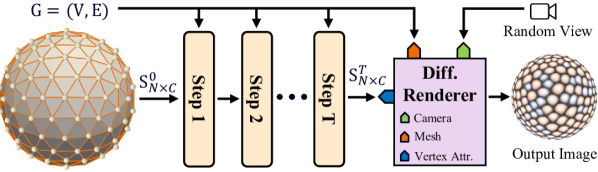
Figure 4: Overview of the texture synthesis process of MeshNCA. Starting with a seed cell states $\mathbf{S}^{0}_{N\times C}$, MeshNCA iteratively updates the cell states by alternating the perception and adaptation stages. The underlying graph topology remains the same across all time steps. The last cell state $\mathbf{S}^{T}_{N\times C}$ and the mesh are then passed to a differentiable renderer and rendered from a random view, resulting in the synthesized image.

MeshNCA acts as a PDE defined on the mesh graph. It evolves over time and produces an ordered series of cell states $\mathbf{S}^{g}=\{{\mathbf{S}^{g_{1}},\mathbf{S}^{g_{2}},\cdots}\}$. Extracting different channels from the cell states, we modify the vertex attributes and alter the appearance of the mesh accordingly, forming a sequence of textured mesh $\mathcal{M}^{g}=\{\mathcal{M}^{g_{1}},\mathcal{M}^{g_{2}},\cdots\}$. Utilizing an interpolation-based differentiable renderer $R$ [5], we convert the textured meshes into image frames as shown in Figure 4. This results in an array of images denoted as $\mathcal{I}^{g}=\{{\mathcal{I}^{g_{1}},\mathcal{I}^{g_{2}},\cdots}\}$. The rendered images are then evaluated against different modalities of the targets, i.e., images or texts, to compute the corresponding appearance losses $\mathcal{L}_{appr-im}$ and $\mathcal{L}_{appr-tx}$. Additionally, we can also impose 2D-only supervision signals on the emergent motion during the training, to synthesize the desired 3D dynamic textures with our MeshNCA model. The motion loss term is denoted as $\mathcal{L}_{mot}$. We elaborate on the loss functions in the following sections.

4.1 Image-guided Training

Leveraging a differentiable renderer, we allow the gradient flow to be backpropagated from the rendered images to MeshNCA parameters. Hence, 2D texture synthesis schemes can be adopted, which typically work by aligning the statistics of deep features of the generated images to those of the target image. Following [33], we utilize a pre-trained VGG16 network [41] to extract the deep features, using the rendered images as input. We denote VGG as $\mathcal{F}_{VGG}$ and the feature map drawn from layer $l$ as $\mathcal{F}^{l}_{VGG}$. Considering that the synthesized 3D texture should be visually analogous to the 2D exemplar image from any specific view, we adopt the multi-view rendering procedure similar to the one in [27]. To ensure the training stability and quality of the results, we implement the style loss proposed by [19]. It consists of a relaxed Wasserstein distance and a moment-matching term. The premise behind this approach is to analytically solve a relaxed optimal transport problem between the extracted features and use this distance as a metric for evaluating style similarity. First, the algorithm converts the deep feature map of size $C\times H\times W$ into a deep feature set via flattening the feature map along the spatial dimensions. This results in the feature set $A$ sourced from the synthesized image and another set $B$ derived from the target image. The relaxed Wasserstein distance $\mathcal{L}_{W}$ and moment-matching term $\mathcal{L}_{M}$ are then defined as:

$$W(A,B) =\frac{1}{|A|}\sum_{i}\mathop{min}\limits_{j}\left(D_{cos}(A_{i},B_{j})\right.$$ (4)

$$\quad\quad\quad\quad\quad\quad\left.+\mathbbm{1}(C=3)D_{euc}(A_{i},B_{j})\right)$$

$$\mathcal{L}_{W}( A,B)=\max\left(W(A,B),W(B,A)\right)$$

$$\mathcal{L}_{M}(A,B)=\frac{1}{C}\left\|\boldsymbol{m}_{A}-\boldsymbol{m}_{B}\right\|_{1}+\frac{1}{C^{2}}\left\|\boldsymbol{T}_{A}-\boldsymbol{T}_{B}\right\|_{1}$$ (5)

Here, $D_{cos}(A_{i},B_{j})$ and $D_{euc}(A_{i},B_{j})$ are the cosine and Euclidean distance between $A_{i}$ and $B_{j}$, respectively. $i,j$ are element indices. $\mathbbm{1}$ is the indicator function that returns $1$ if $A,B$ are the input RGB image and $0$ if they are features extracted from VGG. $\boldsymbol{m}$, $\boldsymbol{T}$ are the mean and covariance matrices of the corresponding sets, respectively. The final loss of image-guided training $\mathcal{L}_{appr-im}$ involves matching multi-layer features. Let $A^{l}_{k}$ and $B^{l}$ be VGG activations extracted by $\mathcal{F}^{l}_{VGG}$ or the input images, where $l$ and $k$ stand for the VGG layer index and view index, respectively. The $l=0$ stands for image input. $\mathcal{L}_{appr-im}$ is then defined as:

$$\mathcal{L}_{appr-im}=\frac{1}{K}\sum^{K}_{k=1}\sum^{L}_{l=0}\left(\mathcal{L}_{W}(A^{l}_{k},B^{l})+\mathcal{L}_{M}(A^{l}_{k},B^{l})\right)$$ (6)

We choose the activations after each convolution layer as well as each pooling layer.

An intriguing property of NCA is that all channels of the cell states share similar structures without imposing external supervision [31]. Such an advantage allows MeshNCA to simultaneously fit multiple texture maps such as albedo, surface normal, roughness, height, and ambient occlusion. We treat each of these texture maps as target texture images and use different channels of the cell states to fit each texture map. We assign 3 channels of the cell states $S_{N\times C}$ to albedo, 3 channels to surface normal, 1 channel to height map, 1 channel to roughness map, and 1 channel to ambient occlusion map. For the single channel texture maps such as the height map, we repeat them 3 times along the channel dimension to get an RGB image and use the same $\mathcal{L}_{appr-im}$ loss. The design of MeshNCA naturally fulfills the requirement of homologous structure between different texture maps, thus allowing for efficient and simultaneous synthesis of textures for physically-based rendering (PBR) applications.

4.2 Text-guided Training

The multi-modal embedding space provided by CLIP [37] renders text-guided image manipulation feasible. In such a training scheme, a text prompt $\mathcal{T}$ is used to describe the desired outcome. Contrary to existing methods in 3D texture synthesis [22, 25, 23], our approach eliminates the need for adding specialized branches to fit the additional geometric vertex attributes. Upon the iteration of MeshNCA, we extract the first 3 channels of the cell states as vertex colors and the 4th channel as the vertex displacement along the surface normal. We constrain the range of the displacement to maintain the overall shape of the mesh. Inspired by [25], we render two images from the same textured mesh, the first using both color and geometric channels, denoted as $\mathcal{I}^{g-color}$, and the second using only the displacement channels by assigning a gray color to vertices, referred to as $\mathcal{I}^{g-geo}$. To prevent potential degeneration of the result, we employ a global augmentation $Aug_{glo}$ and a local augmentation $Aug_{loc}$ to $\mathcal{I}^{g-color}$ and $\mathcal{I}^{g-geo}$ to obtain multiple variations of the synthesized texture. We use the ViT-B/32 model of CLIP, to encode all rendered images to 1D latent codes. An average of these latent codes, taken across all rendering views, provides us with robust representations of the textured mesh in the CLIP’s latent space:

$$\mathcal{R}_{glo}=\frac{1}{K}\sum^{K}_{k=1}CLIP(Aug_{glo}(\mathcal{I}^{g-color}_{k}))$$ (7)

$$\mathcal{R}_{loc}=\frac{1}{K}\sum^{K}_{k=1}CLIP(Aug_{loc}(\mathcal{I}^{g-color}_{k}))$$

$$\mathcal{R}_{loc-geo}=\frac{1}{K}\sum^{K}_{k=1}CLIP(Aug_{loc}(\mathcal{I}^{g-geo}_{k}))$$

where $K$ is the number of rendering views. To further avoid corrupted results, we extend the directional CLIP loss[9, 42] to the 3D domain. Different from the 2D case, the negative components still preserve certain semantic information. Specifically, we define the negative mesh $\mathcal{M}^{neg}$ as the original mesh with a gray color and without any geometric change. The negative images $\mathcal{I}^{neg}$ are rendered from $\mathcal{M}^{neg}$. The negative prompt, $\mathcal{T}^{neg}$, is defined to be the name of the mesh object. The negative images are encoded to latent codes following equation 7 to obtain $\mathcal{R}^{neg}$. The optimization target is the direction between the target prompt latent and negative prompt latent.

$$\Delta\mathcal{R}=\mathcal{R}-\mathcal{R}^{neg},$$ (8)

$$\Delta\mathcal{C}=CLIP(\mathcal{T})-CLIP(\mathcal{T}^{neg})$$

The loss $\mathcal{L}_{appr-tx}$ is defined accordingly:

$$\mathcal{L}_{appr-tx}=\sum_{i}D_{cos}(\Delta\mathcal{R}_{i},\Delta\mathcal{C})$$ (9)

where $i\in\{glo,loc,loc-geo\}$. The $D_{cos}$ is the cosine distance between two 1D vectors.

4.3 Dynamic Texture Synthesis

MeshNCA demonstrates many intriguing emergent properties after training, one of which is spontaneous motion, a characteristic also observed in the NCA model [31, 33]. Pajouheshgar et al. [33] succeeded in controlling the motion generated by NCA via introducing 2D motion training signals. Despite the progress in motion training, guiding the motion on a 3D surface remains a challenging task. First, there is no pre-trained model for estimating 3D speed vectors for each vertex. Moreover, unlike the 2D motion in the vanilla NCA that can happen in any direction, the motion on a 3D mesh is limited to the local tangent space. To solve these problems, we propose to guide the motion via a projected 2D optic flow target.

Let $U:\mathbb{R}^{3}\rightarrow\mathbb{R}^{3}$ to be the user-defined global motion vector field. We evaluate this global motion vector field on the mesh vertices to get per vertex motion $U^{v}\in\mathbb{R}^{N\times 3}$. Given a 3D mesh with vertex normal set $N=\{\hat{n}_{1},\hat{n}_{2},\cdots\}$, we project $U^{v}$ onto the local tangent space of the mesh to obtain the tangent motion vector field for each vertex $U^{p}$.

$$U^{t}_{i}=U^{v}_{i}-(U^{v}_{i}\cdot\hat{n}_{i})\hat{n}_{i},$$ (10)

where $i$ is the vertex index. To allow the cells the be aware of the target motion direction, we set the per-vertex conditional vector, shown in Figure 2 to be $h_{N\times d}=U^{t}$, resulting in Motion Positional Encoding (MPE). Our ablation study in Section 7 shows the necessity of MPE for successfully training MeshNCA to synthesize dynamic textures.

Given a rendering view with camera transformation matrix $CT_{k}$, we project the per-vertex tangent motion vector field $U_{t}$ into the camera-centered coordinate via linear projection $U^{p}_{k}=U^{t}\cdot CT_{k}$. Finally, by fetching the vertex-to-pixel correspondence, we can compute the 2D target motion vector field $U_{k}^{2D}\in\mathbb{R}^{H\times W\times 2}$ for the given view, where $H\times W$ is the render resolution. By keeping the camera parameters unchanged before and after MeshNCA iteration, a pre-trained 2D optic flow estimation network $\mathcal{F}_{OF}$ can predict the view-dependent optic flow for 2D consecutive synthesized images $U^{gen}=\mathcal{F}_{OF}(\mathcal{I}^{g}_{t_{1}},\mathcal{I}^{g}_{t_{2}})$. Here, $t_{1},t_{2}$ are two different time steps along the evolution of MeshNCA, with $t_{1}<t_{2}$. We draw inspiration from [33] to supervise the direction and strength of the generated motion via two losses $\mathcal{L}_{dir}$ and $\mathcal{L}_{str}$, as described in equations 11 and 12, respectively. Our training also incorporates a multi-view strategy to ensure motion consistency on the mesh surface.

$$\mathcal{L}_{dir}=\frac{1}{K}\sum^{K}_{k=1}\frac{1}{HW}\sum_{i,j}D_{cos}(U^{gen}_{ijk},U^{2D}_{ijk}),$$ (11)

$$\mathcal{L}_{str}=\frac{1}{K}\sum^{K}_{k=1}\frac{1}{HW}\sum_{i,j}D_{l1}\left(\frac{T\left\|U^{gen}_{ijk}\right\|_{2}}{t_{2}-t_{1}},\left\|U^{2D}_{ijk}\right\|_{2}\right).$$ (12)

Where $i,j$ are spatial indices and $k$ is the camera view index. Here, $D_{cos}$ and $D_{l1}$ are the cosine and L1 distances, respectively. The constant $T$ regulates the correspondence between the number of MeshNCA steps and the desired motion strength of a single frame. To prioritize the direction matching loss, we formulate the final loss $\mathcal{L}_{mot}$ as:

$$\mathcal{L}_{mot}=\left\{\begin{array}[]{lc}\mathcal{L}_{dir},&\mathcal{L}_{dir}\geq 1.0\\ \left(1.0-\mathcal{L}_{dir}\right)\mathcal{L}_{str}+\gamma\mathcal{L}_{dir},&\mathcal{L}_{dir}<1.0\end{array}\right.$$ (13)

where $\gamma$ is a constant hyperparameter. This approach enables the model to correct the direction first, resulting in more coherent motions.

4.4 Training Graftable models

MeshNCA models exhibit the property of different trained models being able to communicate and form coherent transitions between textures. This property arises only when the models are trained in a specific fashion - a method which resembles the process of ”fine-tuning” as is done with large language and large image models. We consider two NCA to be ”compatible” if neighbouring cells running one of the two rules, on the same substrate (whether a mesh as in MeshNCA or a 2D grid as in the original NCA), exhibit visual coherence in the pattern formed across the boundary between them. See section 3.3 for more details on how to graft trained MeshNCA instances.

The way to encourage two MeshNCA models to be compatible is to first train one on a texture, and then use the resulting converged weights as the initial weights when training a second MeshNCA on a different texture. We observe that when doing so, the training converges faster to the same loss and visual quality compared to training with random initialization. This suggests that the underlying functionality the model learns for producing one texture is at least in part applicable to forming other textures.

5 Experiment

We conduct experiments on the 3D texture synthesis capabilities of MeshNCA, including Image-guided and Text-guided synthesis, in section 5.1 and 5.2, respectively. In all the texture synthesis experiments, MeshNCA shares the same configuration: the single cell state dimensionality $N_{C}=16$, and the output dimensionality of the first layer of MLP being $N_{FC}=128$. This configuration results in a very parameter-efficient model with 12432 trainable parameters. Moreover, we demonstrate that by only imposing motion supervision on the albedo output channels, MeshNCA exhibits the capacity to generate diverse dynamic textures while preserving the coherence between albedo and other texture maps. With the additional motion targets, we set $N_{C}=32$, resulting in 25120 parameters. Furthermore, we summarize several critical properties shared between 2D NCA and MeshNCA and elaborate on our online real-time interactive demo in Section 6. Finally, we perform an ablation study on the MeshNCA architecture and training schemes to demonstrate the necessity of each component in our model.

We use Nvidia Kaolin [5] as our differentiable renderer. All the experiments are performed on an Nvidia-A100 GPU, and use Adam optimizer with an initial learning rate of 0.001. We refer the reader to the supplementary for further training and MeshNCA details.

Guidance	Render Resolution	Camera Distance	# Views
Image	$320\times 320$	2.5	6
Text	$224\times 224$	{2.0, 3.0, 4.0}	5
Image + Motion	$128\times 128$	2.0	6
Text + Motion	$224\times 224$	2.0	8

Table 2: The rendering parameters used in Image-guided, Text-guided synthesis, and corresponding dynamic texture synthesis experiments. For Text-guided experiments, we train each text prompt using 3 different camera distances and pick the one with the lowest loss. The number of views is the $K$ in equation 6.

5.1 Image-guided Synthesis

We collect 72 PBR textures from [1], all of which are available under the CCO license. Each of these textures comes accompanied by albedo, roughness, height, ambient occlusion, and a normal map. We release all the texture maps in our online demo. For fitting the albedo and normal maps, we extract three cell state channels. For learning all other texture maps that are typically represented by a gray-scale image, we repeat one channel of the cell states three times to respect the single-channel nature of the target texture maps. Although we treat the texture map other than albedo as image targets, their values reflect physical properties instead of visual colors. They thus should not be influenced by lighting during training. Hence, we only use ambient lighting in image-guided synthesis experiments. The rendering parameters are given in table 2. The results are shown in figure 5. We provide an online demo available at https://meshnca.github.io/ that incorporates a simple PBR shader to show the effect of applying those texture maps. Note that MeshNCA is only trained on the Icosphere for all of the textures shown in the online demo.

Target Texture Maps		Icosphere Train		Test-time Generalization
Albedo	Attributes	Albedo	Attributes	Albedo	Attributes	Rendering

Figure 5: Results of Image-guided 3D texture synthesis. The attributes are height, normal, roughness, and ambient occlusion maps, from top to bottom, left to right. During training, MeshNCA only encounters the icosphere mesh. At test time, it generalizes to unseen meshes with aligned texture maps. After rendering, the synthesized texture maps show correct shading effects.

5.2 Text-guided Synthesis

We use the ViT-B/32 model for CLIP guidance. Different from the image-guided training, we use spherical harmonic lighting in text-guided synthesis. This is because when being rendered without lighting, the object loses all 3D structures and does not align the prompt that involves the object name. The rendered images are fed into the CLIP model to get embeddings $\mathcal{R}$ in equation 7. The negative components are constructed following the description in section 4.2. All rendering parameters are in table 2. Synthesized textures are demonstrated in figure 6. We provide videos of the results of CLIP-guided MeshNCA training in our demo available at https://meshnca.github.io. Again, MeshNCA never encounters other meshes than the Icosphere. The geometric change also generalizes well to other meshes, confirming that MeshNCA learns the desired geometric texture instead of overfitting to the Icosphere geometry.

Prompts	Train	Test
		Geometry	+Color
Feathers
Cactus
Patchwork Leather
Stained Glass
Bark
Sandstone
Marble

Figure 6: Results of CLIP-guided 3D texture synthesis. MeshNCA only observes icosphere mesh in the training phase. During test time, it generalizes to new meshes both in terms of color and geometric textures.

5.3 3D Dynamic Texture Synthesis

We train MeshNCA to learn the motion defined by a vector field in the 3D space. We manually designed 8 vector fields, including motions with different directions, pattern sink and source, and gradient motion strength. Please read the supplementary materials for a detailed definition and explanation of the motion vector fields. The pre-trained optic-flow estimation network in [43, 33] is used to predict the motion information given two consecutive frames. We feed the network with two rendered images before and after MeshNCA iteration in each epoch to quantify the optic flow on the surface. We set $T=24.0$ in equation 12 for training the motion with the image target, and $T=10.0$ for text-guided synthesis. Figure 7 and 8 show the optic flow estimations for visualizing the generated motions and their corresponding target motions, demonstrating the motion consistency on 3D surfaces. All the 3D vector fields are designed manually. The 2D optic flow visualizations are obtained by placing the mesh center at the origin point and looking from the positive $x$ direction to the negative. The flow visualization follows Baker et al.[2]. We also provide videos generated by MeshNCA with different motion patterns in our demo. We refer readers to the supplementary materials for detailed explanations of the design of these 3D vector fields.

Target Dynamics		Train	Test-time Generalization
Vector Field0	2D Projections	Albedo OF	Attribute OF	Albedo	Albedo OF	Attribute OF

Figure 7: Results of dynamic texture synthesis with image targets. In all visualizations, the camera is fixed to looking at the negative $x$ direction from the positive $x$. The 2D projections of the 3D vector fields onto the camera plane are generated accordingly. During training, motion supervision is only imposed on the albedo channels. Since the channels are implicitly aligned in MeshNCA, all other attributes’ channels follow the same dynamic pattern during test time. Moreover, the learned motion on the icosphere can also be generalized to unseen meshes. We highly encourage the reader to watch the corresponding videos available at https://meshnca.github.io/ to see the dynamic textures.

Prompts	Target Dynamics		Train	Test-time Generalization
	3D Vectors	2D Projections	Color OF	Geometry OF	Color	Color OF	Geometry OF
Jelly Beans
Animal Fur
Colorful Crochet

Figure 8: Results of dynamic texture synthesis under text guidance. The camera constantly looks at the negative $x$ direction from the positive $x$. The seemingly noisy 2D projections are due to the change in mesh geometry. The geometric textures show consistent motion with the color textures, while only the color texture is trained towards the target motion. The synthesized dynamic textures also seamlessly generalize to new meshes without any finetuning. We highly encourage readers to watch the videos released at to see the dynamic textures.

6 MeshNCA Demo

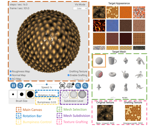
Figure 9: A screenshot of our online demo available at https://meshnca.github.io/. (a) Main Canvas. MeshNCA synthesizes 3D textures on mesh surfaces in real time and generates spontaneous motion. Users can interrupt MeshNCA by simply clicking on the mesh surface, and MeshNCA will self-regenerate. (b) Rotation Bar. The users can control the direction of the pattern arbitrarily by sliding the rotation bar. (c) Bumpiness Control. The bumpiness of the surface, as one of the synthesized properties, can be determined by the users. (d) Mesh Selection. MeshNCA, despite only being trained on the selected icosphere, is capable of generalizing to unseen meshes during testing. (e) Mesh Subdivision. The vertex density of the mesh can be changed and MeshNCA will adapt to the new density, all in real time. (f) Texture Grafting. Users can freely graft two textures together by using the brush tool. We highly encourage the reader to try our online demo.

Our MeshNCA acts as a superset of the 2D NCA proposed in [29]. Hence, it preserves all intriguing test-time properties of the 2D model, facilitating user interactions. We develop an online demo at https://meshnca.github.io/ to show all test-time properties of MeshNCA. Figure 9 marks five critical areas in our online demo that correspond to different MeshNCA properties. We exhibit our trained models from Section 5.1 in our demo. Here, we elaborate on five intriguing properties of our MeshNCA model, including Emergent Spontaneous Motion, Generalization, Self-regeneration, Grafting, and Direction Control.

Emergent Spontaneous Motion: Different from fitting fixed targets with a one-to-one criterion, texture learning typically involves a many-to-one metric. Hence, NCA can spontaneously generate dynamic textures in some cases [31, 33]. More importantly, the motion between NCA steps is coherent instead of fragmented. Such a zero-cost dynamic pattern generation facilitates random motion simulation, dynamic texture synthesis, and creative design in computer graphics[33]. We hypothesize that the motion derives from the spatial gradient information during the Perception stage, explaining why the parametric graph NCA and differentiable reaction-diffusion system lack this property. The intuition here is that local directional information is a necessary condition for the cell to move along certain orientations. The users can directly see the dynamic textures synthesized by MeshNCA in our online demo and can adjust the speed slider to control the motion speed in real time.

Generalization between different topologies: NCA generates the target global pattern solely relying on local cell interaction. Therefore, it possesses generalization ability as long as the local structure remains unchanged. On the 2D regular grid, such a generalization is demonstrated by NCA generating infinite-size images without retraining [33]. In the 3D domain, it is embodied in the generalization between different mesh topologies and vertex densities. The users can select different meshes in the ”Target Mesh” panel to see how MeshNCA generalizes to each of them.

Self-regeneration: NCA is a robust model against severe perturbation at test time [29, 33]. We provide a brush tool with the users to allow deleting vertex colors on the mesh. MeshNCA can promptly respond to such external noise by coherently filling the deleted vertex colors and continuing to synthesize the desired 3D textures. The users can arbitrarily erase parts of the synthesized textures and see how MeshNCA regenerates from the perturbation. Moreover, the users can also change the brush size to adjust the severity of the perturbation.

Grafting: Our trained MeshNCA models, when under the proposed grafting training scheme, can cooperate with each other to synthesize hybrid textures during test time. The users can choose to graft any pair of textures by directly painting on the canvas using the grafting brush tool.

Direction Control: Cells in MeshNCA perceive their surroundings in a direction-aware manner via direction vector projection onto spherical harmonics. An interesting property is that MeshNCA does not overfit the spherical harmonics during training. Instead, it shows rotational equivariance during testing. When the projection bases are rotated, MeshNCA still generates correct but rotated textures. We design the ”Rotation” slider for performing such rotations in our demo.

7 Ablation Study

Parametric and Non-parametric Perception: Spherical Harmonic-based Perception stage lies at the core of MeshNCA. To validate the necessity of our proposed method, we design a parametric perception stage and qualitatively compare the results with MeshNCA’s. Specifically, the modified Perception stage consists of an additional two-layer MLP, taking both features of the center and neighborhood nodes as input. Moreover, to incorporate direction information, the direction vectors between cells are also fed to the MLP. The hidden and output dimensionality is 32 and 64, respectively. The output dimensionality matches the one in our non-parametric Perception stage, ensuring fair comparison. We denote the new model as MeshNCA-P. This configuration results in a 25% increase in trainable parameters compared to MeshNCA. The comparison is given in figure 10. MeshNCA-P fails to generate correct patterns while suffering from lower computational efficiency, hindering further applications.

Target Albedos	Generated Albedos
	MeshNCA	MeshNCA-P

Figure 10: Ablation study on parametric Perception scheme, denoted as MeshNCA-P. While the scheme integrates directional information during the Perception stage, the model did not effectively harness this information, leading to degenerated results.

Degree of Spherical Harmonics: In our method, spherical harmonics of degrees 0 and 1 are used as the projection bases, considering both efficiency and quality. Here, we present the results in figure 11 to demonstrate that the 0-order spherical harmonic is insufficient for generating anisotropic textures while the 2-order one does not show noticeable improvement but increases the size of the model.

Target Albedos	Generated Albedos
	MeshNCA	SH0	SH2

Figure 11: Ablation study on the degree of spherical harmonics. Zero-order spherical harmonics do not possess any direction information and can only synthesize isotropic textures, while the second-order ones do not show noticeable improvement compared to MeshNCA.

Grafting scheme. We graft two MeshNCA models together to produce natural interpolated textures via the same-initialization training scheme. In figure 12, we demonstrate the necessity of our proposed graft training to generate coherent hybrid textures. Either directly training MeshNCA without proper initialization or naive linear interpolation fails to ensure a smooth transition between the two grafted textures.

Target Albedos	Texture Mask	Interpolated Albedos
		Same-Init	Diff-Init	Direct Interpolation

Figure 12: Ablation study on the graft training scheme. ”Same-init” means that two MeshNCA models share the same initialization while ”Diff-init” indicates different ones. Moreover, the naive linear interpolation between two textures is denoted as ”Direct Interpolation”. Our training scheme, ”Same-init”, produces coherent transition between two textures and results in a new hybrid texture, while the other two schemes fail.

Motion Positional Encoding: Our MeshNCA is accompanied with Motion Positional Encoding (MPE) when performing dynamic texture synthesis, introduced in Section 4.3. These cell-wise target dynamics guide each cell to move in the desired direction. A lack of such information can lead to sub-optimal dynamic textures. We conduct ablation studies on MPE and present the result in figure 13.

Target Dynamics		MPE	Plain
Vectors	Projections

Figure 13: Ablation study on Motion Positional Encoding. The model without the encoding is denoted as Plain. The Plain model struggles to accurately capture intricate motions, including rotation or those exhibiting non-uniform speed changes across vertices. Such a limitation is exhibited both during the training on icosphere and at test time with new meshes. The underlying textures of the motion demonstration are Sci-fi_Wall_010 and Sci-Fi_Wall_012 in our collected dataset.

8 Limitations

MeshNCA suffers from certain limitations. While different cell state channels share similar structures, misalignment happens on a few textures, leading to wrong shading effects. Such a failure might be attributed to implicit supervision of the structural alignment of different texture maps. Moreover, since our MeshNCA framework assigns texture attributes to vertices of the mesh, the quality of the synthesized 3D texture depends on the input mesh quality. To achieve high quality, our model requires high poly meshes with uniformly distributed vertices on the surface. Furthermore, MeshNCA is sensitive to certain rendering parameters. Variations in aspects such as rendering resolution and camera distance can influence the outcomes to a certain extent. Consequently, the framework might yield sub-optimal results if these parameters are not well selected. Finally, MeshNCA is agnostic to the semantic structures of the underlying 3D meshes and textures the surface without semantic meanings. We provide examples of the inferior cases in our supplementary materials.

9 Conclusion

We propose MeshNCA, a Cellular-Automata-based model for real-time and interactive 3D texture synthesis on meshes. Our model can generalize to any mesh in test time while only being trained on an icosphere mesh. Furthermore, MeshNCA exhibits several intriguing test-time properties, including spontaneous motion, self-regeneration, texture grafting, and texture direction control–all of which can be seamlessly executed in real-time on consumer devices through our online interactive demo. By employing a message-passing scheme, our proposed spherical-harmonics-based filters extend the convolution-based perception filters of conventional NCA to accommodate more general non-grid structures like meshes. Our model can be trained with both image targets or text prompt guidance to synthesize the desired pattern, broadening its range of applications. Moreover, we demonstrate that MeshNCA, equipped with our proposed Motion Positional Encoding, can be trained with motion supervision to synthesize dynamic 3D textures that generalize across meshes. Additionally, we conceptualize a procedure to seamlessly graft multiple MeshNCA models, enabling the synthesis of hybrid textures that exhibit characteristics of two texture instances.

References

- [1] 3DTextures.me. Free seamless PBR textures with Diffuse, Normal, Displacement, Occlusion and Roughness Maps. https://3dtextures.me/.
- [2] Simon Baker, Daniel Scharstein, JP Lewis, Stefan Roth, Michael J Black, and Richard Szeliski. A database and evaluation methodology for optical flow. International Journal of Computer Vision, 92(1):1–31, 2011.
- [3] Alexey Bokhovkin, Shubham Tulsiani, and Angela Dai. Mesh2tex: Generating mesh textures from image queries. arXiv preprint arXiv:2304.05868, 2023.
- [4] Dave Zhenyu Chen, Yawar Siddiqui, Hsin-Ying Lee, Sergey Tulyakov, and Matthias Nießner. Text2tex: Text-driven texture synthesis via diffusion models. arXiv preprint arXiv:2303.11396, 2023.
- [5] Wenzheng Chen, Huan Ling, Jun Gao, Edward Smith, Jaakko Lehtinen, Alec Jacobson, and Sanja Fidler. Learning to predict 3d objects with an interpolation-based differentiable renderer. Advances in neural information processing systems, 32, 2019.
- [6] Alexei A Efros and Thomas K Leung. Texture synthesis by non-parametric sampling. In Proceedings of the Seventh IEEE International Conference on Computer Vision, volume 2, pages 1033–1038. IEEE, 1999.
- [7] Kurt W Fleischer, David H Laidlaw, Bena L Currin, and Alan H Barr. Cellular texture generation. In Proceedings of the 22nd annual conference on Computer graphics and interactive techniques, pages 239–248, 1995.
- [8] WT Freeman and Ce Liu. Markov random fields for super-resolution and texture synthesis. Advances in Markov Random Fields for Vision and Image Processing, 1(155-165):3, 2011.
- [9] Rinon Gal, Or Patashnik, Haggai Maron, Amit H Bermano, Gal Chechik, and Daniel Cohen-Or. Stylegan-nada: Clip-guided domain adaptation of image generators. ACM Transactions on Graphics (TOG), 41(4):1–13, 2022.
- [10] Leon Gatys, Alexander S Ecker, and Matthias Bethge. Texture synthesis using convolutional neural networks. Advances in Neural Information Processing Systems, 28, 2015.
- [11] Stéphane Gobron and Norishige Chiba. 3d surface cellular automata and their applications. The Journal of Visualization and Computer Animation, 10(3):143–158, 1999.
- [12] Daniele Grattarola, Lorenzo Livi, and Cesare Alippi. Learning graph cellular automata. Advances in Neural Information Processing Systems, 34:20983–20994, 2021.
- [13] Paul Guerrero, Miloš Hašan, Kalyan Sunkavalli, Radomír Mĕch, Tamy Boubekeur, and Niloy J Mitra. Matformer: A generative model for procedural materials. ACM Transactions on Graphics, 41(4), 2022.
- [14] Jorge Gutierrez, Julien Rabin, Bruno Galerne, and Thomas Hurtut. On demand solid texture synthesis using deep 3d networks. In Computer Graphics Forum, volume 39, pages 511–530. Wiley Online Library, 2020.
- [15] Jianwei Han, Kun Zhou, Li-Yi Wei, Minmin Gong, Hujun Bao, Xinming Zhang, and Baining Guo. Fast example-based surface texture synthesis via discrete optimization. The Visual Computer, 22:918–925, 2006.
- [16] Philipp Henzler, Niloy J Mitra, and Tobias Ritschel. Learning a neural 3d texture space from 2d exemplars. In Proceedings of the IEEE/CVF Conference on Computer Vision and Pattern Recognition, pages 8356–8364, 2020.
- [17] Yiwei Hu, Julie Dorsey, and Holly Rushmeier. A novel framework for inverse procedural texture modeling. ACM Transactions on Graphics (ToG), 38(6):1–14, 2019.
- [18] Yiwei Hu, Paul Guerrero, Miloš Hašan, Holly Rushmeier, and Valentin Deschaintre. Generating procedural materials from text or image prompts. arXiv preprint arXiv:2304.13172, 2023.
- [19] Nicholas Kolkin, Jason Salavon, and Gregory Shakhnarovich. Style transfer by relaxed optimal transport and self-similarity. In Proceedings of the IEEE/CVF Conference on Computer Vision and Pattern Recognition, pages 10051–10060, 2019.
- [20] Johannes Kopf, Chi-Wing Fu, Daniel Cohen-Or, Oliver Deussen, Dani Lischinski, and Tien-Tsin Wong. Solid texture synthesis from 2d exemplars. ACM Transactions on Graphics (Proceedings of SIGGRAPH 2007), 26(3):2:1–2:9, 2007.
- [21] Sylvain Lefebvre and Hugues Hoppe. Appearance-space texture synthesis. ACM Trans. Graph., 25(3):541–548, jul 2006.
- [22] Jiabao Lei, Yabin Zhang, Kui Jia, et al. Tango: Text-driven photorealistic and robust 3d stylization via lighting decomposition. Advances in Neural Information Processing Systems, 35:30923–30936, 2022.
- [23] Yiwei Ma, Xiaioqing Zhang, Xiaoshuai Sun, Jiayi Ji, Haowei Wang, Guannan Jiang, Weilin Zhuang, and Rongrong Ji. X-mesh: Towards fast and accurate text-driven 3d stylization via dynamic textual guidance. arXiv preprint arXiv:2303.15764, 2023.
- [24] Stéphane Mérillou and Djamchid Ghazanfarpour. A survey of aging and weathering phenomena in computer graphics. Computers & Graphics, 32(2):159–174, 2008.
- [25] Oscar Michel, Roi Bar-On, Richard Liu, Sagie Benaim, and Rana Hanocka. Text2mesh: Text-driven neural stylization for meshes. In Proceedings of the IEEE/CVF Conference on Computer Vision and Pattern Recognition, pages 13492–13502, 2022.
- [26] Alexander Mordvintsev and Eyvind Niklasson. nca: Texture generation with ultra-compact neural cellular automata. arXiv preprint arXiv:2111.13545, 2021.
- [27] Alexander Mordvintsev, Nicola Pezzotti, Ludwig Schubert, and Chris Olah. Differentiable image parameterizations. Distill, 3(7):e12, 2018.
- [28] Alexander Mordvintsev, Ettore Randazzo, and Eyvind Niklasson. Differentiable programming of reaction-diffusion patterns. In ALIFE 2022: The 2022 Conference on Artificial Life. MIT Press, 2021.
- [29] Alexander Mordvintsev, Ettore Randazzo, Eyvind Niklasson, and Michael Levin. Growing neural cellular automata. Distill, 2020. https://distill.pub/2020/growing-ca.
- [30] J von Neumann. Theory of self-reproducing automata. Mathematics of Computation, 21:745, 1966.
- [31] Eyvind Niklasson, Alexander Mordvintsev, Ettore Randazzo, and Michael Levin. Self-organising textures. Distill, 6(2):e00027–003, 2021.
- [32] Michael Oechsle, Lars Mescheder, Michael Niemeyer, Thilo Strauss, and Andreas Geiger. Texture fields: Learning texture representations in function space. In Proceedings of the IEEE/CVF International Conference on Computer Vision, pages 4531–4540, 2019.
- [33] Ehsan Pajouheshgar, Yitao Xu, Tong Zhang, and Sabine Süsstrunk. Dynca: Real-time dynamic texture synthesis using neural cellular automata. In Proceedings of the IEEE/CVF Conference on Computer Vision and Pattern Recognition, pages 20742–20751, 2023.
- [34] Darwyn R Peachey. Solid texturing of complex surfaces. In Proceedings of the 12th annual conference on Computer graphics and interactive techniques, pages 279–286, 1985.
- [35] Ken Perlin. An image synthesizer. ACM Siggraph Computer Graphics, 19(3):287–296, 1985.
- [36] Tiziano Portenier, Siavash Arjomand Bigdeli, and Orcun Goksel. Gramgan: Deep 3d texture synthesis from 2d exemplars. Advances in Neural Information Processing Systems, 33:6994–7004, 2020.
- [37] Alec Radford, Jong Wook Kim, Chris Hallacy, Aditya Ramesh, Gabriel Goh, Sandhini Agarwal, Girish Sastry, Amanda Askell, Pamela Mishkin, Jack Clark, et al. Learning transferable visual models from natural language supervision. In International conference on machine learning, pages 8748–8763. PMLR, 2021.
- [38] Elad Richardson, Gal Metzer, Yuval Alaluf, Raja Giryes, and Daniel Cohen-Or. Texture: Text-guided texturing of 3d shapes. arXiv preprint arXiv:2302.01721, 2023.
- [39] Liang Shi, Beichen Li, Miloš Hašan, Kalyan Sunkavalli, Tamy Boubekeur, Radomir Mech, and Wojciech Matusik. Match: Differentiable material graphs for procedural material capture. ACM Transactions on Graphics (TOG), 39(6):1–15, 2020.
- [40] Yawar Siddiqui, Justus Thies, Fangchang Ma, Qi Shan, Matthias Nießner, and Angela Dai. Texturify: Generating textures on 3d shape surfaces. In European Conference on Computer Vision, pages 72–88. Springer, 2022.
- [41] Karen Simonyan and Andrew Zisserman. Very deep convolutional networks for large-scale image recognition. In Yoshua Bengio and Yann LeCun, editors, 3rd International Conference on Learning Representations, ICLR 2015, San Diego, CA, USA, May 7-9, 2015, Conference Track Proceedings, 2015.
- [42] Yiren Song. Cliptexture: Text-driven texture synthesis. In Proceedings of the 30th ACM International Conference on Multimedia, pages 5468–5476, 2022.
- [43] Matthew Tesfaldet, Marcus A Brubaker, and Konstantinos G Derpanis. Two-stream convolutional networks for dynamic texture synthesis. In Proceedings of the IEEE Conference on Computer Vision and Pattern Recognition, pages 6703–6712, 2018.
- [44] Alan Mathison Turing. The chemical basis of morphogenesis. Bulletin of Mathematical Biology, 52(1):153–197, 1990.
- [45] Greg Turk. Generating textures on arbitrary surfaces using reaction-diffusion. Acm Siggraph Computer Graphics, 25(4):289–298, 1991.
- [46] Greg Turk. Texture synthesis on surfaces. In Proceedings of the 28th annual conference on Computer graphics and interactive techniques, pages 347–354, 2001.
- [47] Li-Yi Wei and Marc Levoy. Texture synthesis over arbitrary manifold surfaces. In Proceedings of the 28th annual conference on Computer graphics and interactive techniques, pages 355–360, 2001.
- [48] Lexing Ying, Aaron Hertzmann, Henning Biermann, and Denis Zorin. Texture and shape synthesis on surfaces. In Rendering Techniques 2001: Proceedings of the Eurographics Workshop in London, United Kingdom, June 25–27, 2001 12, pages 301–312. Springer, 2001.
- [49] Jiaxuan You, Zhitao Ying, and Jure Leskovec. Design space for graph neural networks. Advances in Neural Information Processing Systems, 33:17009–17021, 2020.
- [50] Jingdan Zhang, Kun Zhou, Luiz Velho, Baining Guo, and Heung-Yeung Shum. Synthesis of progressively-variant textures on arbitrary surfaces. In ACM SIGGRAPH 2003 Papers, pages 295–302. 2003.