Signal Processing Meets SGD: From Momentum to Filter

Abstract

In deep learning, stochastic gradient descent (SGD) and its momentum-based variants are widely used in optimization algorithms, they usually face the problem of slow convergence. Meanwhile, existing adaptive learning rate optimizers accelerate convergence but often at the expense of generalization ability. We demonstrate that the adaptive learning rate property impairs generalization. To address this contradiction, we propose a novel optimization method that aims to accelerate the convergence rate of SGD without loss of generalization. This approach is based on the idea of reducing the variance of the historical gradient, enhancing the first-order moment estimation of the SGD by applying Wiener filtering theory, and introducing a time-varying adaptive weight. Experimental results show that SGDF achieves a trade-off between convergence and generalization compared to state-of-the-art optimizers.

1 Introduction

In the training process, the optimizer serves as the model’s key component. The optimizer refines and adjusts model parameters to guarantee that the model is able to recognize the underlying patterns of the data. Besides updating weights, its responsibility includes strategically navigating models through complex loss landscapes(Du & Lee, 2018) to find regions with the best generalization (Keskar et al., 2016). The chosen optimizer dramatically affects training efficiency: model convergence speed, generalization performance, and resilience to data distribution shifts (Bengio & Lecun, 2007). A poor optimizer choice may lead to stopping in suboptimal regions or failing to converge, but a suitable one can accelerate learning and guarantee robust performance (Ruder, 2016). Hence, continually refining optimization algorithms is crucial for enhancing machine learning model capabilities.

In deep learning, Stochastic Gradient Descent (SGD) (Monro, 1951) and its variants like momentum-based SGD (Sutskever et al., 2013), Adam (Kingma & Ba, 2014), and RMSprop (Hinton, 2012) have secured prominent roles. Despite their substantial contributions to deep learning, these methods have inherent drawbacks. These techniques primarily exploit first-order moment estimation and frequently overlook the historical gradient’s pivotal influence on current parameter adjustment. So they will result in training instability or terrible generalization, particularly with high-dimensional, non-convex loss functions common in deep learning (Goodfellow et al., 2016). Such characteristics render adaptive learning rate methods prone to entrapment in sharp local minima, which might devastate the model’s generalization capability.

To strike an effective trade-off between convergence speed and generalization capability, this paper introduces a novel optimization method called SGDF. SGDF incorporates filter theory from signal processing to enhance first-moment estimation, achieving a balance between historical and current gradient estimates. Through its adaptive weighting mechanism, SGDF precisely adjusts gradient estimates throughout the training process, thus accelerating model convergence while maintaining a certain level of generalization ability.

Initial evaluations demonstrate that SGDF surpasses many traditional adaptive learning rate and variance reduction optimization methods in various benchmark datasets, particularly in terms of speeding up convergence and maintain generalization. This indicates that SGDF successfully navigates the trade-off between quickening convergence speed and preserving generalization capability. By achieving this balance, SGDF offers a more efficient and robust optimization option for training deep learning models.

The main contributions of this paper can be summarized as follows:

• We propose an optimizer that integrates both historical and current gradient data to compute the gradient’s variance estimate in order to address the classical SGD method’s slow convergence.

• Our method leverage a first-moment filter estimation, our approach markedly enhances the adaptive optimization algorithm’s generalization, surpassing traditional momentum strategies.

• We propose an innovative theoretical framework and give upper bounds on the expectation of Lipschitz’s continuous constant $\mathbb{E}\left[L_{T}\right]$ for different algorithms called sharpness upper bound that elucidates the key relation between the stochastic sampling gradient and the convergence of the algorithm to a flat minimum. This lays a theoretical foundation for capturing the generalization of optimizers.

2 Related Works And Motivations

Convergence: Variance reduction to Adaptive In the early stages of development of deep learning, optimization algorithms focused on reducing the variance of gradient estimation(Johnson & Zhang, 2013; Defazio et al., 2014; Schmidt et al., 2017; Balles & Hennig, 2018) to achieve a linear convergence rate. Subsequently, the emergence of adaptive learning rate methods(Duchi et al., 2011; Dozat, 2016; Zeiler, 2012) marked an important shift in optimization algorithms. Though SGD and its variants have advanced in many applications, they come with inherent limitations. They often oscillate or get trapped in sharp minima (Wilson et al., 2017). Although it makes models reach low training loss, such minima frequently fail to generalize effectively to new data (Hardt et al., 2015; Xie et al., 2022). This generalization effectiveness becomes worse in the high-dimensional, non-convex terrains characteristic of deep learning settings (Dauphin et al., 2014; Lucchi et al., 2022).

Fig. 1 provides a visualization to illustrate the behavior of various optimization algorithms. The figure clearly depicts the loss landscapes for Adam, SGD-M, and our proposed optimizer. Notably, the visualization reveals that Adam is more prone to converge to sharper minima.

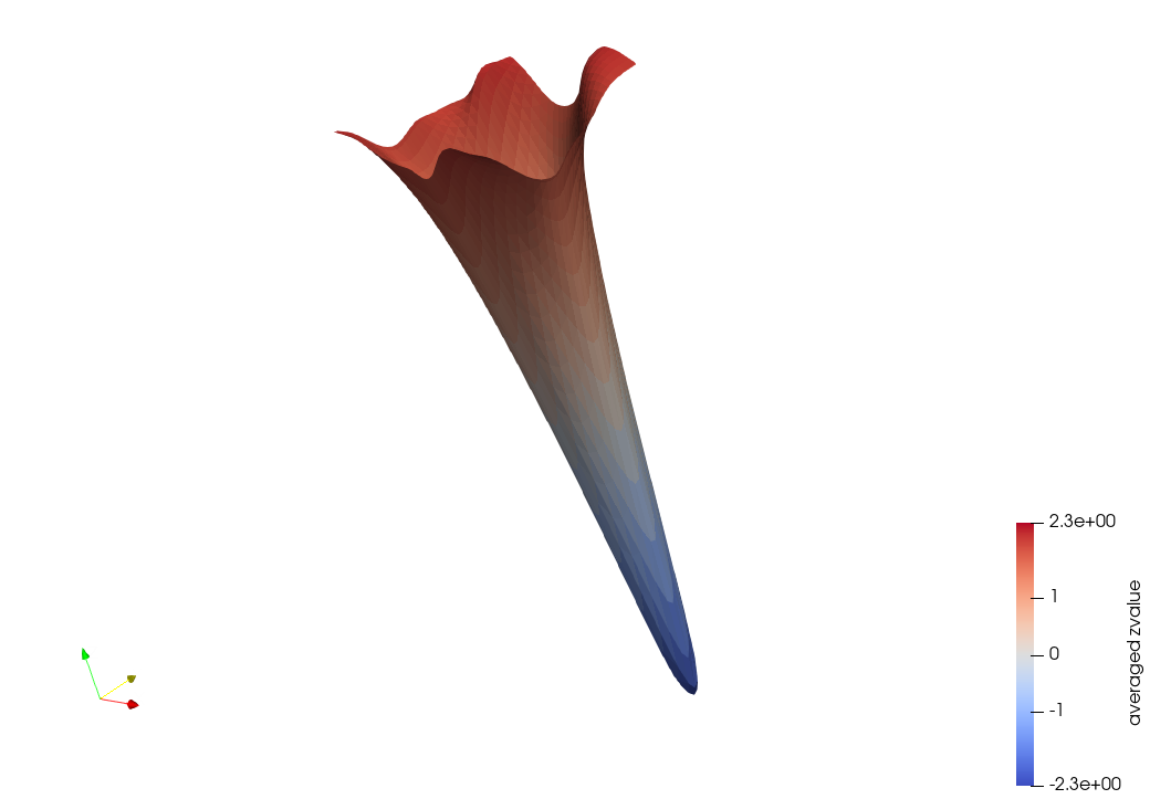
(a) Adam

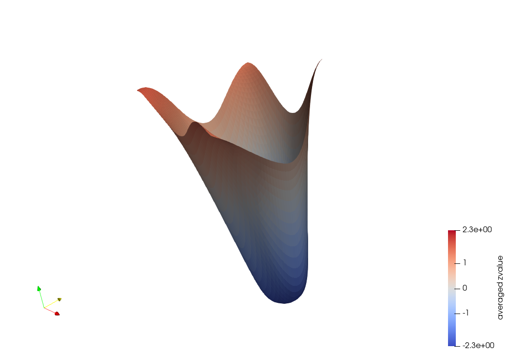
(b) SGD

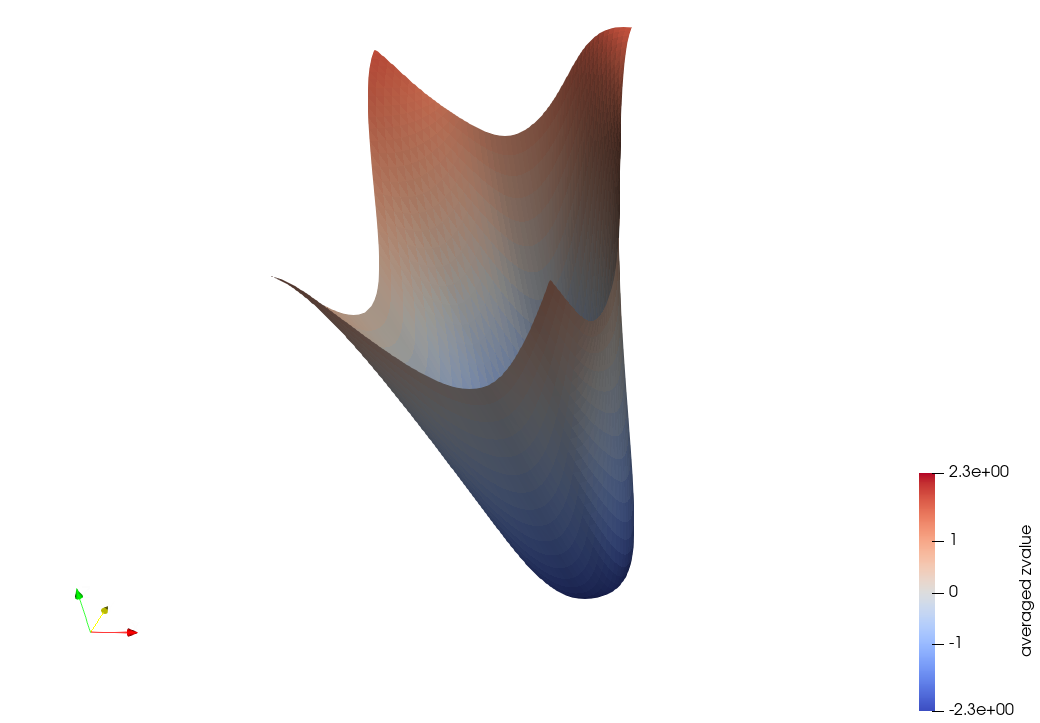
(c) SGDM

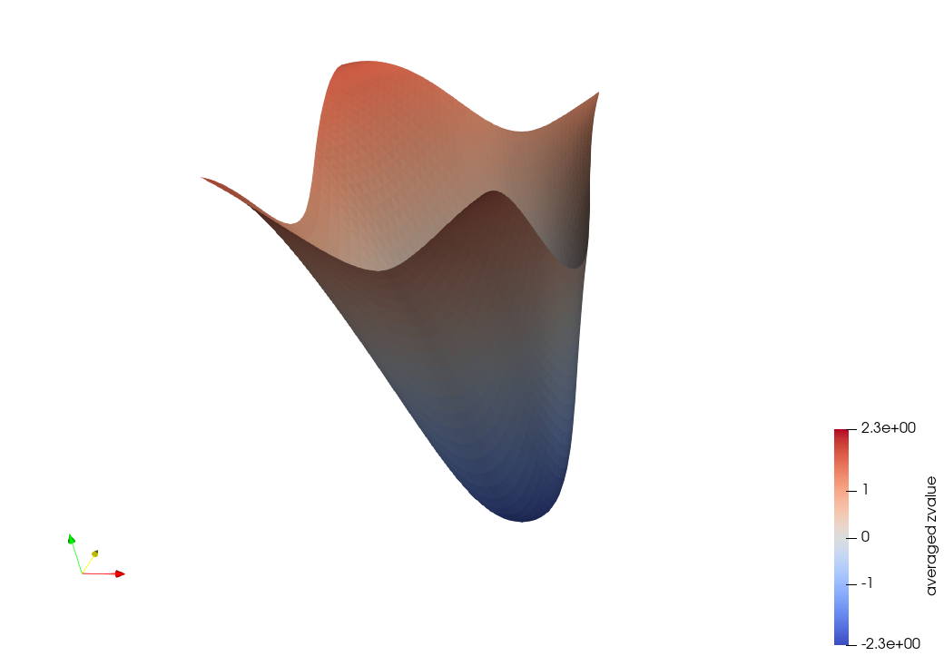
(d) SGDF

Figure 1: Visualization of loss landscape.

Generalization: Sharp and Flat Solutions The generalization ability of a deep learning model depends heavily on the nature of the solutions found during the optimization process. (Keskar et al., 2017) demonstrated experimentally that flat minima generalize better than sharp minima. (Foret et al., 2021) theoretically demonstrated that the generalization error of smooth minima is lower than that of sharp minima on test data, and further proposed to optimize the zero-order smoothness. (Zhang et al., 2023) improves the SAM by simultaneously optimizing the prediction error and the number of paradigms of the maximum gradient in the neighborhood during the training process. Adai(Xie et al., 2020) aims to balance the exploration and exploitation in the optimization process by adjusting the inertia of each parameter update. This adaptive inertia mechanism helps the model to avoid falling into sharp local minima. However, it is criticized that the convergence curve of Adai is similar to SGD, which means that the speed is not improved. The form of Adai’s adaptive momentum inertia weights is similar to the method in this paper, but we adopt the idea of minimizing the mean-square error (Kay, 1993) to estimate the gradient fundamentally and improved convergence.

Second-Order and Filter Methods The recent integration of second-order information into optimization problems has become increasingly popular(Liu et al., 2023; Yao et al., 2020b). Methods such as Kalman Gradient Descent (Kalman, 1960) incorporate second-order curvature information(Vuckovic, 2018; Ollivier, 2019). The KOALA algorithm (Davtyan et al., 2022) claims that optimizer need be qualified with loss adaptivity. It adjusts learning rates in terms of both gradient magnitudes and the loss landscape’s curvature.

For the sake of low training error and robust generalization, models must address the bias-variance tradeoff (Geman et al., 2014). The trajectory of an optimizer within the loss landscape is a representation of this trade-off. An erratic trajectory might lead to sharp, poorly-generalizing minima, while a conservative approach could result in the model getting stuck in broad, suboptimal plateaus (Zhang et al., 2016; Yang et al., 2023).

Our research is motivated by these challenges and the observed behavior of different optimizers, particularly the tendency of Adam to converge to sharper minima compared to methods like SGD. This observation raises an important question: what causes Adam’s convergence to sharper solutions, and is it possible to achieve a trade-off between convergence speed and generalization? Although previous studies offer valuable insights, a notable gap remains in fully understanding optimizer behavior. To bridge this gap, we provide both theoretical and empirical perspectives on how optimizers navigate the loss landscape and investigate the impact of such behavior on model generalization (Chandramoorthy et al., 2022).

3 Main Result

3.1 Preliminaries

Assumption 3.1.

Let $f:\mathbb{R}^{n}\rightarrow\mathbb{R}$ be a differentiable function. The gradient of $f$ is considered Lipschitz continuous if there exists a non-negative constant $L$ (referred to as the Lipschitz constant of the gradient) such that for all $\theta_{1},\theta_{2}\in\mathbb{R}^{n}$, the following inequality holds:

$$\|\nabla f(\theta_{1})-\nabla f(\theta_{2})\|\leq L\|\theta_{1}-\theta_{2}\|$$ (1)

This constant $L$ describes the rate of change or the bound on the slope of the gradient. A small $L$ implies that the gradient of the function changes slowly, whereas a large $L$ might suggest rapid changes in the gradient in some regions.

Definition 3.2.

Let $f_{t}(\theta_{t})$ be the loss at time $t$ and $f_{t}(\theta^{*})$ be the loss of the best possible strategy at the same time. The cumulative regret $R(T)$ at time $T$ is defined as:

$$R(T)=\sum_{t=1}^{T}f_{t}(\theta_{t})-f_{t}(\theta^{*})$$ (2)

Notations: We use $g_{t}$ to denote the gradient computed from the dataset $\mathcal{D}$ based on random sample sampling at each iteration $t$. $L_{t}$ is the Lipschitz constant over the range of two neighboring iterations of the gradient descent algorithm. We use $\mathbb{E}\left[L_{T}\right]$ to approximate $L_{\mathcal{N}(\theta_{T+1})}$ to denote the upper bound of sharpness in the neighbourhood of the convergence parameter $\theta_{T+1}$ of the algorithm. The vector $g_{1:t,i}\in\mathbb{R}^{t}$ contains the values of all gradients in the $i$th dimension up to iteration $t$, i.e., $g_{1:t,i}=\left[g_{1,i},g_{2,i},\cdots,g_{t,i}\right]$. We define $\mathbb{E}\left[\left\|\nabla f(\theta_{T+1})-\nabla f(\theta_{1})\right\|\right]=\delta$. We denote the distance measure between the parameters $\theta$ as $D$ and the gradient bounded by $G$.

3.2 $L_{t}$ lower bound for different algorithms

Theorem 3.3.

Let $f:\mathbb{R}^{n}\rightarrow\mathbb{R}$ be a differentiable function whose gradient satisfies the Lipschitz continuity condition. In consecutive SGD iterations, the following inequality holds:

$$\frac{\mathbb{E}\left[\left\|\nabla f\left(\theta_{t+1}\right)-\nabla f\left(\theta_{t}\right)\right\|\right]}{\alpha\mathbb{E}\left[\left\|g_{t}\right\|\right]}\leq\mathbb{E}\left[L_{t}\right].$$ (3)

Then, the following inequality relation holds:

$$L_{\mathcal{N}(\theta_{T+1})}\approx\mathbb{E}\left[L_{T}\right] \leq\frac{\delta}{\alpha\mathbb{E}\left[\left\|\nabla g_{T}\right\|\right]}$$ (4)

Theorem 3.3 provides insights into the smoothness characteristics of the Stochastic Gradient Descent (SGD) algorithm. It suggests that the sharpness of the convergence region in SGD can be quantitatively assessed using the Lipschitz continuity constant $\mathbb{E}\left[L_{T}\right]$. This constant reflects the bounded rate of gradient change, which is integral to understanding the algorithm’s behavior during optimization. A smaller $\mathbb{E}\left[L_{T}\right]$ indicates a flatter convergence region, implying more stability and possibly better generalization in the model trained by SGD. Conversely, a larger $\mathbb{E}\left[L_{T}\right]$ may indicate a sharper, less stable convergence region. This understanding is crucial for fine-tuning SGD and its variants, as it emphasizes the importance of the gradient’s magnitude and its rate of change for efficient and stable convergence.

Similarly, we also derive the expectation of the momentum term when considering the update rule for the momentum method:

$$\mathbb{E}[v_{t+1}]=\alpha\sum_{i=0}^{t}\beta^{i}\mathbb{E}[g_{t+1-i}]$$ (5)

Corollary 3.4.

Given the momentum method, the lower bound of  $\mathbb{E}[L_{T}]$ after accumulating over $T$ time steps is:

$$L_{\mathcal{N}(\theta_{T+1})}\approx\mathbb{E}\left[L_{T}\right]\leq\frac{\delta}{\alpha\sum_{i=0}^{T}\beta^{i}\mathbb{E}\left[\left\|g_{T+1-i}\right\|\right]}$$ (6)

If we assume that  $\mathbb{E}[g_{t+1-i}]$ is the same constant M for all $i$, then the summation part of the original formula can be simplified by a geometric progression of summation formulas:.

$$L_{\mathcal{N}(\theta_{T+1})}\approx\mathbb{E}\left[L_{T}\right]\leq\frac{\delta(1-\beta)}{\alpha M(1-\beta^{T+1})}$$ (7)

Corollary 3.4 reveals the expectation of the Lipschitz continuity condition $\mathbb{E}\left[L_{t}\right]$ bounds in optimizers using the Momentum Method (SGDM). In contrast to SGD, the momentum approach updates the parameters by taking into account the cumulative effect of past gradients. This approach not only relies on current gradient information, but also integrates the direction and magnitude of historical gradients. Such integration allows the algorithm to jump from local minima to flatter regions more efficiently, reducing the likelihood of convergence to sharp minima. As a result, momentum methods are better able to balance the speed of convergence with the quality of the solution when dealing with complex or noisy lossy surfaces, often leading to flatter convergence regions and more stable learning dynamics.

Therefore, it can be suggested that employing momentum often results in a reduced threshold for $\mathbb{E}\left[L_{t}\right]$, facilitating faster convergence and superior solutions, particularly in the presence of complex loss landscapes.

Consider the update rules of the Adam method, wherein the update of parameters depends not only on the first moment (i.e., mean) of the gradient but also on its second moment (or an approximation of unbiased variance). Specifically, through the utilization of the mean $\widehat{m}_{t}$ and unbiased variance $\widehat{v}_{t}$, we arrive at the following approximation for the stochastic gradient:

$$\theta_{t+1}=\theta_{t}-\alpha\frac{\mathbb{E}\left[g_{t}\right]}{\sqrt{\mathbb{E}^{2}\left[g_{t}\right]+\mathrm{Var}(g_{t})}}$$ (8)

Corollary 3.5.

The lower bound for $\mathbb{E}[L_{T}]$ when using the Adam optimization method, considering the stochastic gradient, is as follows:

$$L_{\mathcal{N}(\theta_{T+1})}\approx\mathbb{E}\left[L_{T}\right]\leq\frac{\delta\sqrt{\mathbb{E}^{2}\left[\left\|g_{T}\right\|\right]+\mathrm{Var}\left(\left\|g_{T}\right\|\right)}}{\alpha\mathbb{E}\left[\left\|g_{T}\right\|\right]}$$ (9)

However, it is critical to note that the adaptive nature of the Adam method may lead it to converge to sharper minima compared to standard SGD, potentially resulting in less robust solutions. Moreover, the variance of the gradient can significantly influence Adam’s updates, with unbounded variance potentially leading to instability(Liu et al., 2019; Xiong et al., 2020).

Various Adam variants(Chen et al., 2018; Liu et al., 2019; Luo et al., 2019; Zhuang et al., 2020) improve the generalization performance by adjusting the learning rate, and in particular they try to improve the optimization by reducing the impact of the learning rate on the upper bounds of the sharpness of the loss function process stability and solution robustness. These variants aim to alleviate some of the problems observed in the vanilla Adam method, such as convergence to undesirable sharp minima or instability in the face of high variance in the gradient estimate.

Assumption 3.6.

Let $g_{t}$ be a stochastic gradient, If the variance of the random variable $g_{t}$, denoted as $\mathrm{Var}(g_{t})$, converges to a certain Cramér-Rao lower bound $\mathcal{C}$, i.e.,

$$\lim_{t\to\infty}\mathrm{Var}(g_{t})=\mathcal{C}$$ (10)

Remark 3.7.

As discussed in Section 4.3, the Wiener filtering method introduced in this study effectively reduces the variance of the gradient in stochastic gradient estimation. This filtering approach ensures that the variance of the estimated gradient diminishes over iterations by linearly combining current noisy gradient observations with historical estimates.

Theorem 3.8.

Then, as $t$ increases, we can be certain that $g_{t}$ will unbiasedly approach its expected value $\mathbb{E}[g_{t}]$, formally stated as:

$$\lim_{t\to\infty}P\left(g_{t}-\mathbb{E}[g_{t}]=0\right)=1$$ (11)

Theorem 3.8 demonstrates that in SGD, the stochastic gradient’s variance converges to a fixed lower bound. This convergence facilitates an unbiased probabilistic approximation of the gradient to its expected value. According to (Johnson & Zhang, 2013; Defazio et al., 2014; Schmidt et al., 2017), the variance is gradually reduced at a rate of $\xi^{t-1},\xi\in(0,1)$. This approach rapidly decreases the initial variance, facilitating linear convergence rate, as noted in (Bottou et al., 2018). Our approach ensures the algorithm’s stability and rapid convergence while maintaining a level of noise. This noise aids in circumventing local optima, leading to solutions with superior generalization capabilities as described in (Yang et al., 2022).

To validate our theory, we examined the Hessian matrix, which describes the second-order curvature of the loss function in parameter space. Within this framework, we emphasize the Lipschitz constant, as it sets an upper limit on gradient variation. Specifically, a significant Hessian eigenvalue suggests areas of high curvature, potentially indicative of rapid gradient shifts, which are directly associated with the Lipschitz constant (Caldarola et al., 2022).

We computed the Hessian spectrum of ResNet-18 trained on the Cifar100 dataset for 200 epochs. These trainings used SGD, SGDM, Adam and SGDF, which are four optimization methods. We use power iteration (Yao et al., 2018) to compute the top eigenvalues of Hessian and Hutchinson’s method (Yao et al., 2020a) to compute the Hessian trace. We present histograms that illustrate the distribution of the top-50 Hessian eigenvalues for each optimization method in Fig. 2.

\begin{overpic}[width=99.73074pt]{experiments/hessian_spectra/SGDF.png} \put(60.0,52.0){\scriptsize Trace: 184.14 } \put(60.0,42.0){\scriptsize$\lambda_{\text{max}}$: 17.03} \end{overpic}

(a) SGDF

\begin{overpic}[width=99.73074pt]{experiments/hessian_spectra/SGDM.png} \put(60.0,52.0){\scriptsize Trace: 344.75} \put(60.0,42.0){\scriptsize$\lambda_{\text{max}}$: 26.51} \end{overpic}

(b) SGDM

\begin{overpic}[width=99.73074pt]{experiments/hessian_spectra/SGD.png} \put(60.0,52.0){\scriptsize Trace: 267.64} \put(60.0,42.0){\scriptsize$\lambda_{\text{max}}$: 30.07} \end{overpic}

(c) SGD

\begin{overpic}[width=99.73074pt]{experiments/hessian_spectra/Adam.png} \put(60.0,52.0){\scriptsize Trace: 3376.97} \put(60.0,42.0){\scriptsize$\lambda_{\text{max}}$: 183.11} \end{overpic}

(d) Adam

Figure 2: Histogram of Top 50 Hessian Eigenvalues

Our experiments ensure that all methods perform similarly on the training set. However, the difference in test accuracy is significant. Lower maximum eigenvalues and traces of the Hessian matrix are associated with better test accuracy, demonstrating the generalization advantage of the flat solution. Our method maintains similar generalization performance to SGD-M while accelerating convergence.

Finally, we provide the convergence property of SGDF as shown in Theorem 3.9

Theorem 3.9.

Assume that the function $f_{t}$ has bounded gradients, $\|\nabla f_{t}(\theta)\|_{2}\leq G$, $\|\nabla f_{t}(\theta)\|_{\infty}\leq G_{\infty}$ for all $\theta\in\mathbb{R}^{d}$ and distance between any $\theta_{t}$ generated by SGDF is bounded, $\|\theta_{n}-\theta_{m}\|_{2}\leq D$, $\|\theta_{m}-\theta_{n}\|_{\infty}\leq D_{\infty}$ for any $m,n\in\{1,...,T\}$, and $\beta_{1},\beta_{2}\in[0,1)$. Let $\alpha_{t}=\sqrt{\alpha/t}$. SGDF achieves the following guarantee, for all $T\geq 1$:

$$R(T)\leq \frac{D^{2}}{\alpha}\sum_{i=1}^{d}\sqrt{T}+\frac{2D_{\infty}G_{\infty}}{1-\beta_{1}}\sum_{i=1}^{d}\left\|g_{1:T,i}\right\|_{2}$$ (12)

$$+\frac{2\alpha G_{\infty}^{2}(1+(1-\beta_{1})^{2})}{\sqrt{T}(1-\beta_{1})^{2}}\sum_{i=1}^{d}\left\|g_{1:T,i}\right\|_{2}^{2}$$

The assumptions in Theorem 3.9 are common and standard when analyzing convergence of convex functions via SGD-based methods(Kingma & Ba, 2014; Reddi et al., 2019).

4 Wiener Filter Estimate Gradient

Due to the adaptive learning rate, the algorithm may converge to sharp minima, potentially resulting in less robust solutions. Therefore based on the above Theorem 3.8, we present SGDF and subsequently discovered that it shares the same underlying principles as Wiener filtering. SGDF minimize the mean squared error(Wiener, 1950), which effectively reduces the variance of the estimated gradient distribution. This design ensures that the algorithm achieves a trade-off between convergence speed and generalization.

4.1 SGDF details

Algorithm 1 SGDF, Wiener Filter Estimate Method. All operations are element-wise.

Input: $\{\alpha_{t}\}^{T}_{t=1}$: step size,

$\{\beta_{1},\beta_{2}\}$: attenuation coefficient,

$\theta_{0}$: initial parameter,

$f(\theta)$: stochastic objective function

Output: $\theta_{T}$: resulting parameters.

Init: $m_{0}\leftarrow 0$, $v_{0}\leftarrow 0$

while $t=1$ to $T$ do

       $g_{t}\leftarrow\nabla_{\theta}f_{t}(\theta_{t-1})$ (Calculate gradients w.r.t. stochastic objective at timestep $t$) $m_{t}\leftarrow\beta_{1}m_{t-1}+(1-\beta_{1})g_{t}$ (Calculate momentum) $s_{t}\leftarrow\beta_{2}s_{t-1}+(1-\beta_{2})(g_{t}-m_{t})^{2}$ (Calculate variance) $\widehat{m}_{t}\leftarrow\dfrac{m_{t}}{1-\beta_{1}^{t}}$,$\widehat{s}_{t}\leftarrow\dfrac{s_{t}}{1-\beta_{2}^{t}}$(Bias correction) $K_{t}\leftarrow\dfrac{\widehat{s}_{t}}{\widehat{s}_{t}+(g_{t}-\widehat{m}_{t})^{2}}$ (Calculate Estimate Gain) $\widehat{g}_{t}\leftarrow\widehat{m}_{t}+K_{t}(g_{t}-\widehat{m}_{t})$ (Update gradient estimation) $\theta_{t}\leftarrow\theta_{t-1}-\alpha_{t}\widehat{g}_{t}$ (Update parameters)

return $\theta_{T}$

In the SGDF algorithm, the term $s_{t}$ serves as an important indicator. It is approximated by the exponential moving average of the squared difference between the current gradient $g_{t}$ and its corresponding momentum $m_{t}$. This acts as a proxy for long-term gradient variations, with its weight modulated by the hyperparameter $\beta_{2}$. In essence, $s_{t}$ can be interpreted as an estimation of the variance or inherent uncertainty that captures the scale of fluctuations in the gradient.

Regarding the gradient, at any given time step $t$, $g_{t}$ denotes the stochastic gradient with respect to our objective function. Concurrently, $m_{t}$ provides an approximation of the history of the gradient, as it denotes the exponential moving average of the gradient, accumulating past gradient values in a weighted manner. As a result, the term $g_{t}-m_{t}$ emerges as a key concept. It can be seen as the residual or deviation of the gradient during the optimization process. This deviation essentially shows how much the current gradient diverges from its historical trend. From a Bayesian perspective, this deviation mirrors the uncertainty or intrinsic noise involved in the estimation of the instantaneous gradient, which can be mathematically represented as $p(g_{t}\mid\mathcal{D})\sim\mathcal{N}(g_{t};m_{t},\sigma_{t}^{2})$(Liu et al., 2019).

In the context of SGDF, the gain $K_{t}$ is used to balance the contribution between the current observed gradient $g_{t}$ and the past corrected gradient $\widehat{m}_{t}$, thereby providing a refined gradient estimate. The range of $K_{t}$ is typically between 0 and 1. It provides a mechanism by which we can balance confidence between the current stochastic gradient and the past corrected gradient. This trade-off is particularly important when dealing with highly noisy gradients or in complex optimisation landscapes. In many deep learning scenarios, gradients are often influenced by various factors, leading to significant noise. By introducing a compensation factor $K_{t}$, this noise can be offset to some extent, resulting in a more stable gradient direction, faster convergence and improved model performance. The calculation of $K_{t}$ is based on the dynamics of $s_{t}$ and $g_{t}-m_{t}$. Its aim is to minimize the expected variance of the corrected gradient estimate $\widehat{g}_{t}$, which is achieved optimal linear estimation under noisy conditions.

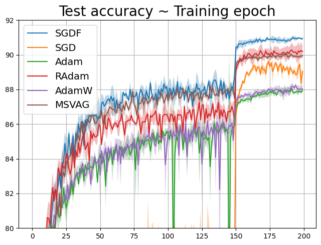
(a) VGG11 on Cifar10

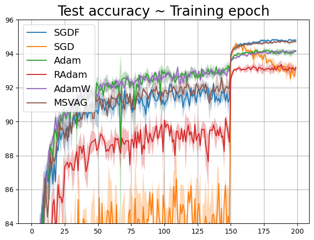
(b) ResNet34 on Cifar10

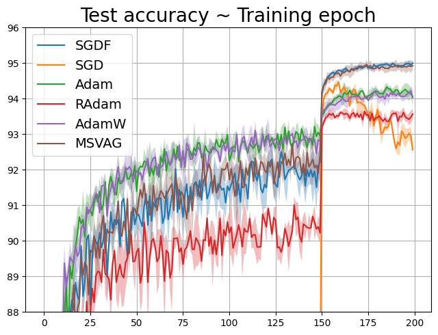
(c) DenseNet121 on Cifar10

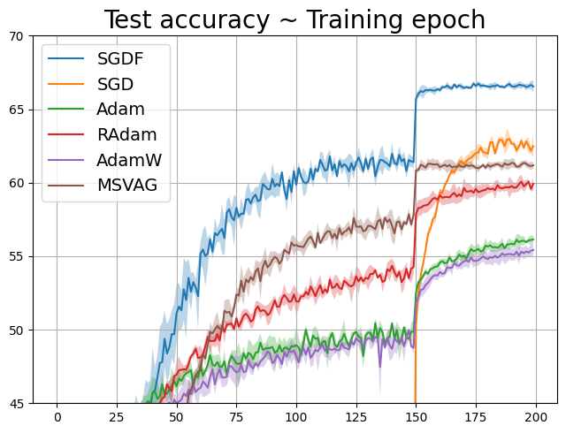
(d) VGG11 on Cifar100

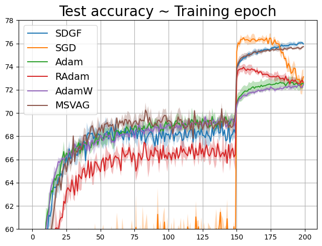
(e) ResNet34 on Cifar100

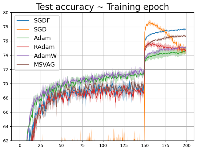
(f) DenseNet121 on Cifar100

Figure 3: Test accuracy ([$\mu\pm\sigma$]) on Cifar.

4.2 Detailed Derivation of the Wiener Gain $K_{t}$

The core concept behind the Wiener filter is to provide a linear estimate of a desired signal sequence from another related sequence, so as to minimize the mean square error between the estimated and desired sequences. The Wiener filter operates based on the principles of orthogonality and relies heavily on the statistical properties of the signals involved.

In the field of optimization, particularly gradient descent, the terrain of the loss landscape can introduce complexities in the trajectory the gradient takes. This can be visualized as noise that perturbs the gradient descent path. Formally, we represent this noise-affected gradient as $g_{t}=\nabla f(\theta_{t})+\zeta_{t}$.

The derivation for $K_{t}$ starts by understanding its role as a balancing factor between the first and second moments of the gradient. This balancing act ensures that gradient updates are more aligned with the true gradient direction.

Starting with the variance of the corrected gradient, we have:

$$\mathrm{Var}(\widehat{g}_{t})=(1-K_{t})^{2}\mathrm{Var}(\widehat{m}_{t})+K_{t}^{2}\mathrm{Var}(g_{t})$$ (13)

The objective is to minimize $\mathrm{Var}(\hat{g}_{t})$. Differentiating with respect to $K_{t}$ and equating to zero, the optimal $K_{t}$ is found:

$$\frac{\partial\mathrm{Var}(\widehat{g}_{t})}{\partial K_{t}} =2(1-K_{t})\mathrm{Var}(\widehat{m}_{t})-2K_{t}\mathrm{Var}(g_{t})=0$$ (14)

Solving for $K_{t}$, we get $K_{t}=\frac{\mathrm{Var}(\widehat{m}_{t})}{\mathrm{Var}(\widehat{m}_{t})+\mathrm{Var}(g_{t})}$. Simplifying further, the equation becomes:

$$K_{t}=\frac{\widehat{s}_{t}}{\widehat{s}_{t}+(g_{t}-\widehat{m}_{t})^{2}}.$$ (15)

From the above derivations, it’s evident how the principles of Wiener filtering play a significant role in optimization algorithms, guiding the gradient updates in the presence of noisy landscapes.

Table 1: Top-1, 5 accuracy of ResNet18 on ImageNet. ^{∗  †  ‡} is reported in (Zhuang et al., 2020; Chen et al., 2018; Liu et al., 2019).

Method	SGDF	SGD	AdaBound	Yogi	MSVAG	Adam	RAdam	AdamW
Top-1	70.23	70.23†	68.13†	68.23†	65.99∗	63.79† (66.54‡)	67.62‡	67.93†
Top-5	89.55	89.40†	88.55†	88.59†	-	85.61†	-	88.47†

Table 2: The mAP (higher is better) on PASCAL VOC using Faster-RCNN+FPN.

Method	SGDF	SGD	Adam	AdamW	RAdam
mAP	83.81	80.43	78.67	78.48	75.21

4.3 Fusion of Gaussian Distributions

When the Wiener filter is applied, the gradient estimates converge to a Gaussian distribution. The properties of the Wiener filter ensure that the estimated gradient is a linear combination of the current noisy gradient observation $g_{t}$ and the prior gradient estimate $\widehat{g}_{t-1}$. These two components are assumed to have Gaussian distributions, where $g_{i}\sim\mathcal{N}\left(\mu,\sigma^{2}\right)$. Hence, their fusion by the Wiener filter naturally ensures that the fused estimate $\widehat{g}_{t}$ is also Gaussian.

Let’s denote the standard deviations of these Gaussians as $\sigma_{1}$ and $\sigma_{2}$ respectively. The standard deviation of the resulting Gaussian distribution is given by the relation:

$$\sigma^{\prime}=\sqrt{\frac{\sigma_{1}^{2}\sigma_{2}^{2}}{\sigma_{1}^{2}+\sigma_{2}^{2}}}$$ (16)

When using Wiener filtering, fusing two Gaussian distributions results in a gradual decrease in the variance of the estimated gradient its variance. This reduction in variance is important for the optimization process because it means that the gradient estimate becomes more accurate and stable over time. The reduced variance reduces the uncertainty in the gradient update process and helps to achieve smoother optimization paths, which is especially important when dealing with complex loss landscapes in deep learning models.

5 Experiments

In this study, We focus on these following tasks: Image Classification. We employed the VGG (Simonyan & Zisserman, 2014), ResNet (He et al., 2016), and DenseNet (Huang et al., 2017) models for image classification tasks on the Cifar dataset(Krizhevsky et al., 2009). We evaluated and compared the performance of SGDF with other optimizers such as SGD, Adam, RAdam (Liu et al., 2019), and AdamW (Loshchilov & Hutter, 2017), all of which were implemented based on the official Pytorch library. Additionally, we further tested the performance of SGDF on the ImageNet dataset (Deng et al., 2009) using the ResNet model. Object Detection. Object detection was performed on the PASCAL VOC dataset(Everingham et al., 2010) using Faster-RCNN (Ren et al., 2015) integrated with FPN. For hyper-parameter tuning related to image classification and object detection, refer to (Zhuang et al., 2020). Image Generation. Wasserstein-GAN (WGAN)(Arjovsky et al., 2017) on Cifar10 dataset. Extended Experiments. Wiener filtering combined with Adam boost generalization. Experiment results are given in the following subsection.

Cifar10/100 Experiments. Initially, we trained on the Cifar10 and Cifar100 datasets using the VGG, ResNets, and DenseNet models, and assessed the performance of the SGDF optimizer. We conducted a search for optimal hyperparameters (Zhuang et al., 2020). For SGD, the momentum rate was set to 0.9, and the initial learning rate was 0.1. For Adam, RAdam, and AdamW, we used the default parameters: $\alpha=0.001$, $\beta_{1}=0.9$, $\beta_{2}=0.999$, and $\epsilon=10^{-8}$. For SGDF and MSVAG, the parameters were set as: $\alpha=0.3$, $\beta_{1}=0.9$, $\beta_{2}=0.999$, and $\epsilon=10^{-8}$. In Cifar10/100 experiments, the batch size was 128 with basic data augmentation techniques such as random horizontal flip and random cropping (with a 4-pixel padding). We conducted training for 200 epochs, and the learning rate was multiplied by a factor of 0.1 at the 150th epoch. For all optimizers, an typically weight decay of $5\times 10^{-4}$ was introduced (Loshchilov & Hutter, 2017). The results show the mean and standard deviation of 3 runs, visualized as curve graphs in Fig. 3.

As Fig. 3 shows, it is evident that the SGDF optimizer exhibited convergence speeds comparable to adaptive optimization algorithms. In addition, SGDF final test set accuracy was either better than or equal to that achieved by SGD.

ImageNet Experiments. In this section, we used the ResNet18 model to train on the ImageNet dataset. Due to extensive computational demands, we did not conduct an exhaustive hyperparameter search for other optimizers and chose to use the best-reported parameters from (Chen et al., 2018; Liu et al., 2019). We trained for 100 epochs using a batch size of 256 and applied basic data augmentation strategies such as random cropping and random horizontal flipping. The learning rate was multiplied by a factor of 0.1 every 30 epochs. For SGD, we set the initial learning rate to 0.1. For SGDF optimizer, we set $\alpha$=0.5, $\beta_{1}$=0.5. The results are shown in Tab. 1. Detailed training and test curves we place in the Fig. 7. In addition to eliminate the effect of learning rate scheduling, with reference to (Chen et al., 2023; Zhang et al., 2023) we used cosine learning rate scheduling and trained 90 epochs on ResNet18, 34, 50 models. The results are shown in Tab. 3. Experiments on the ImageNet dataset show that the SGDF has improved convergence speed and achieves similar accuracy to SGD on the test set.

Table 3: Cosine learning rate scheduling train ImageNet. ^∗ is reported in (Zhang et al., 2023)

Model	ResNet18	ResNet34	ResNet50
SGDF	70.16	73.37	76.03
SGD	69.80	73.26	76.01∗

Object Detection. We do object detection experiments on the PASCAL VOC dataset (Everingham et al., 2010). The model we used here is pre-trained on COCO dataset (Lin et al., 2014) and the pre-trained model is from the official website. We train this model on the VOC2007 and VOC2012 trainval dataset (17K) and evaluate on the VOC2007 test dataset (5K). The model we used is Faster-RCNN (Ren et al., 2015) + FPN. The backbone is ResNet50 (He et al., 2016). Results are summarized in Tab. 2. As we except, SGDF outperforms other. These results also illustrates that our method is still efficient in object detection tasks.

Image Generation. Generative adversarial networks Stability of optimizers is important in practice such as training of GANs. The training of a GAN alternates between generator and discriminator in a mini-max game, and is typically unstable; SGD often generates mode collapse, and adaptive methods such as Adam and RMSProp are recommended in practice. Therefore, training of GANs is a good test for the stability.

We experiment with one of the most widely used models, the Wasserstein-GAN with gradient penalty (WGAN-GP)(Salimans et al., 2016) using a small model with vanilla CNN generator. Using popular optimizer(Luo et al., 2019; Zaheer et al., 2018; Balles & Hennig, 2018; Bernstein et al., 2020), we train the model for 100 epochs, generate 64,000 fake images from noise, and compute the Frechet Inception Distance (FID)(Heusel et al., 2017) between the fake images and real dataset (60,000 real images). FID score captures both the quality and diversity of generated images and is widely used to assess generative models (lower FID is better). For SGD and MSVAG, we report results from (Zhuang et al., 2020). We perform 5 runs of experiments, and report the results in Fig. 4.

Experimental results show that SGDF significantly improves WGAN-GP model training, attaining a FID score higher than vanilla SGD and surpassing most adaptive optimization methods. The use of a Wiener filter in SGDF smoothly updates gradients, reducing training oscillations and aiding in addressing the issue of pattern collapse.

Extended Experiment. In our study, we performed comparative experiments on the Cifar100 dataset, evaluating both the vanilla Adam algorithm and its combination with the Wiener Filter. The detailed test curves are presented in Fig. 9. It shows that the performance of the adaptive learning rate algorithms is improved by our first moment filter estimation.

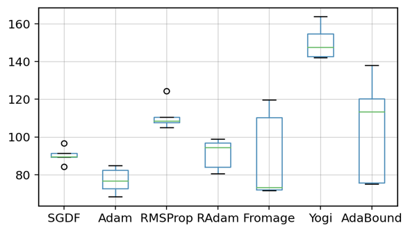
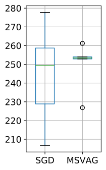
Figure 4: FID score of WGAN-GP.

6 Conclusion

In this work, we introduce SGDF, a novel optimization method that enhances the gradient estimation process by exploiting the information variance of the historical gradient combined with the current gradient. Through extensive experiments using various deep learning architectures on benchmark datasets, we demonstrate the superior performance of SGDF compared to other state-of-the-art optimizers.

Our theoretical framework elucidates properties of the convergence location of the algorithm, insights that are crucial to the field of deep learning, re-emphasising the importance of flat solutions for improving generalisation. However, it can be observed from the experiments that SGDF does not significantly improve the generalization compared to SGD. Improving the generalization while maintaining the convergence speed is a major issue for future work.

Another important direction is about the excellent performance of Adam’s algorithm in the field of NLP. It has been suggested in the literature that the reason why Adam’s algorithm is able to converge quickly may be related to its insensitivity to local smoothness(Zhang et al., 2019; Wang et al., 2022). This provides inspiration to delve into the applicability of optimization algorithms in different tasks and domains. The performance and applicability of different optimization algorithms in specific application domains are further explored to understand how they work and how they can be further optimized.

In conclusion, optimization algorithms in deep learning are an evolving field and there are still many issues that need to be addressed and investigated. The further development of the field will be promoted through in-depth exploration of the performance, theoretical foundations, and relationship of the algorithms to specific tasks, and continuous improvement of the convergence speed and generalisation ability of the algorithms.

Appendix A Proofs

A.1 Theorem proof.

Definition A.1.

The expectation of the norm difference between $\nabla f(\theta_{T+1})$ and $\nabla f(\theta_{1})$ is $\delta$, where $\delta$ is a constant. We can represent:

$$\mathbb{E}\left[\left\|\nabla f(\theta_{T+1})-\nabla f(\theta_{1})\right\|\right]=\delta$$ (17)

Assumption A.2.

(Lipschitz continuous). If $f$ is Lipschitz continuous.

$$\|\nabla f(\theta_{1})-\nabla f(\theta_{2})\|\leq L\|\theta_{1}-\theta_{2}\|,\forall\theta_{1},\theta_{2}\in\mathbb{R}^{d}$$ (18)

Theorem A.3.

Under Assumption A.2 and in accordance with Definition A.1, consider a loss function $f$ where $g_{t}$ represents the gradient computed through stochastic sampling from the dataset at each iteration. For the update rule of stochastic gradient descent, the following inequality relation holds:

$$\mathbb{E}\left[L_{T}\right] \leq\frac{\delta}{\alpha\mathbb{E}\left[\left\|\nabla g_{T}\right\|\right]}$$ (19)

Proof. For the update rule of SGD:

$$\theta_{t+1}=\theta_{t}-\alpha g_{t}.$$ (20)

Consider adjacent step iterations, We can derive:

$$\mathbb{E}\left[\left\|\nabla f\left(\theta_{t+1}\right)-\nabla f\left(\theta_{t}\right)\right\|\right]\leq\alpha\mathbb{E}\left[L_{t}\right]\mathbb{E}\left[\left\|g_{t}\right\|\right]$$ (21)

We first apply the logarithm to the whole term and then add up the result.

For the original inequality

$$\frac{\mathbb{E}\left[\left\|\nabla f\left(\theta_{t+1}\right)-\nabla f\left(\theta_{t}\right)\right\|\right]}{\alpha\mathbb{E}\left[\left\|g_{t}\right\|\right]}\leq\mathbb{E}\left[L_{t}\right]$$ (22)

Start by taking logarithms on both sides of the inequality:

$$\log\left(\frac{\mathbb{E}\left[\left\|\nabla f\left(\theta_{t+1}\right)-\nabla f\left(\theta_{t}\right)\right\|\right]}{\alpha\mathbb{E}\left[\left\|g_{t}\right\|\right]}\right)\leq\log\left(\mathbb{E}\left[L_{t}\right]\right)$$ (23)

By the logarithmic property, the above inequality can be further transformed into:

$$\log\left(\mathbb{E}\left[\left\|\nabla f\left(\theta_{t+1}\right)-\nabla f\left(\theta_{t}\right)\right\|\right]\right)-\log\left(\alpha\mathbb{E}\left[\left\|g_{t}\right\|\right]\right)\leq\log\left(\mathbb{E}\left[L_{t}\right]\right)$$ (24)

Now add up from t=1 to T:

$$\sum_{t=1}^{T}\left(\log\left(\mathbb{E}\left[\left\|\nabla f\left(\theta_{t+1}\right)-\nabla f\left(\theta_{t}\right)\right\|\right]\right)-\log\left(\alpha\mathbb{E}\left[\left\|g_{t}\right\|\right]\right)\right)\leq\sum_{t=1}^{T}\log\left(\mathbb{E}\left[L_{t}\right]\right)$$ (25)

Next, you can replace the difference of successive gradients with the difference in gradients between $\mathbf{\theta}_{T+1}$ and $\mathbf{\theta}_{1}$ using a triangular inequality. This will find an upper bound for the numerator. Consider the cumulative inequality we have just obtained:

$$\sum_{t=1}^{T}\left(\log\left(\mathbb{E}\left[\left\|\nabla f\left(\theta_{t+1}\right)-\nabla f\left(\theta_{t}\right)\right\|\right]\right)-\log\left(\alpha\mathbb{E}\left[\left\|\nabla f_{s}\left(\theta_{t}\right)\right\|\right]\right)\right)\leq\sum_{t=1}^{T}\log\left(\mathbb{E}\left[L_{t}\right]\right)$$ (26)

We wish to replace the numerator of the left-hand side with $\mathbb{E}\left[\left\|\nabla f\left(\theta_{T+1}\right)-\nabla f\left(\theta_{1}\right)\right\|\right]$. We already know that the difference in each successive gradient will be less than this according to the trigonometric inequality. Therefore, we have:

$$\mathbb{E}\left[\left\|\nabla f\left(\theta_{t+1}\right)-\nabla f\left(\theta_{t}\right)\right\|\right]\leq\mathbb{E}\left[\left\|\nabla f\left(\theta_{T+1}\right)-\nabla f\left(\theta_{1}\right)\right\|\right]$$ (27)

Considering that logarithmic functions are increasing functions, we can apply to the above inequality to get:

$$\log\left(\mathbb{E}\left[\left\|\nabla f\left(\theta_{t+1}\right)-\nabla f\left(\theta_{t}\right)\right\|\right]\right)\leq\log\left(\mathbb{E}\left[\left\|\nabla f\left(\theta_{T+1}\right)-\nabla f\left(\theta_{1}\right)\right\|\right]\right)$$ (28)

Replacing this back into our cumulative inequality, we get:

$$\sum_{t=1}^{T}\log\left(\mathbb{E}\left[L_{t}\right]\right) \leq\sum_{t=1}^{T}\left(\log\left(\mathbb{E}\left[\left\|\nabla f\left(\theta_{T+1}\right)-\nabla f\left(\theta_{1}\right)\right\|\right]\right)-\log\left(\alpha\mathbb{E}\left[\left\|g_{t}\right\|\right]\right)\right)$$ (29)

$$\sum_{t=1}^{T}\log\left(\mathbb{E}\left[L_{t}\right]\right) \leq\sum_{t=1}^{T}\log\left(\frac{\left(\mathbb{E}\left[\left\|\nabla f\left(\theta_{T+1}\right)-\nabla f\left(\theta_{1}\right)\right\|\right]\right)}{\left(\alpha\mathbb{E}\left[\left\|g_{t}\right\|\right]\right)}\right)$$

After applying the exponential function, we get

$$e^{\sum_{t=1}^{T}\log\left(\mathbb{E}\left[L_{t}\right]\right)}\leq e^{\sum_{t=1}^{T}\log\left(\frac{\mathbb{E}\left[\left\|\nabla f\left(\theta_{T+1}\right)-\nabla f\left(\theta_{1}\right)\right\|\right]}{\alpha\mathbb{E}\left[\left\|g_{t}\right\|\right]}\right)}$$ (30)

Since $e^{\log x}=x$ , this simplifies to:

$$\prod_{t=1}^{T}\mathbb{E}\left[L_{t}\right]\leq\prod_{t=1}^{T}\frac{\mathbb{E}\left[\left\|\nabla f\left(\theta_{T+1}\right)-\nabla f\left(\theta_{1}\right)\right\|\right]}{\alpha\mathbb{E}\left[\left\|g_{t}\right\|\right]}$$ (31)

After dividing the inequality at time $T$ by the inequality at time $T-1$, we have iquequality of $\mathbb{E}[L_{T}]$:

$$\mathbb{E}\left[L_{T}\right]\leq\frac{\mathbb{E}\left[\left\|\nabla f\left(\theta_{T+1}\right)-\nabla f\left(\theta_{1}\right)\right\|\right]}{\alpha\mathbb{E}\left[\left\|g_{T}\right\|\right]}$$ (32)

In accordance with Definition A.1, which states that the expectation of the norm difference between $\nabla f(\theta_{T+1})$ and $\nabla f(\theta_{1})$ is $\delta$, the cumulative inequality can be represented as follows:

$$\mathbb{E}\left[L_{T}\right] \leq\frac{\delta}{\alpha\mathbb{E}\left[\left\|g_{T}\right\|\right]}$$ (33)

Corollary A.4.

Under Assumption A.2 and in accordance with Definition A.1, considering a loss function $f$ and its stochastic gradient $g_{t}$, the following inequality relation holds for the update rule of the momentum method:

$$\mathbb{E}\left[L_{T}\right]\leq\frac{\delta}{\alpha\sum_{i=0}^{T}\beta^{i}\mathbb{E}\left[\left\|g_{T+1-i}\right\|\right]}$$ (34)

Proof. The basic update rule for the momentum method is:

$$v_{t+1} =\beta v_{t}+\alpha g_{t}$$ (35)

$$\theta_{t+1} =\theta_{t}-v_{t+1}$$

Consider the desired update rule:

$$\mathbb{E}\left[v_{t+1}\right]=\beta\mathbb{E}\left[v_{t}\right]+\alpha\mathbb{E}\left[g_{t}\right]$$ (36)

Since we already know that $\mathbb{E}\left[g_{t}\right]$ is the expectation of the gradient, we only need to consider the expectation of $v_{t}$. When we initialise, $v_{0}=0$, then:

$$\mathbb{E}\left[v_{1}\right] =\alpha\mathbb{E}\left[g_{1}\right]$$ (37)

$$\mathbb{E}\left[v_{2}\right] =\beta\alpha\mathbb{E}\left[g_{1}\right]+\alpha\mathbb{E}\left[g_{2}\right]$$

$$\mathbb{E}\left[v_{3}\right] =\beta^{2}\alpha\mathbb{E}\left[g_{1}\right]+\beta\alpha\mathbb{E}\left[g_{2}\right]+\alpha\mathbb{E}\left[g_{3}\right]$$

As can be seen, at each step the previous gradient is multiplied by an additional $\beta$ factor. At the $t$ time step, the updated expectation can be written as:

$$\mathbb{E}\left[v_{t}\right]=\alpha\sum_{i=0}^{t-1}\beta^{i}\mathbb{E}\left[g_{t-i}\right]$$ (38)

Given an update rule:

$$\mathbb{E}\left[v_{t+1}\right] =\beta\mathbb{E}\left[v_{t}\right]+\alpha\mathbb{E}\left[g_{t}\right]$$ (39)

At the $t$ time step, the desired update can be expressed as:

$$\mathbb{E}\left[v_{t}\right] =\alpha\sum_{i=0}^{t-1}\beta^{i}\mathbb{E}\left[g_{t-i}\right]$$ (40)

Replacing the above equation, we get:

$$\mathbb{E}\left[v_{t+1}\right] =\beta\left(\alpha\sum_{i=0}^{t-1}\beta^{i}\mathbb{E}\left[g_{t-i}\right]\right)+\alpha\mathbb{E}\left[g_{t}\right]$$ (41)

Expanding and adjusting the index of the summation, we get:

$$\mathbb{E}\left[v_{t+1}\right] =\alpha\beta\sum_{i=0}^{t-1}\beta^{i}\mathbb{E}\left[g_{t-i}\right]+\alpha\mathbb{E}\left[g_{t}\right]$$ (42)

$$=\alpha\sum_{i=1}^{t}\beta^{i}\mathbb{E}\left[g_{t+1-i}\right]+\alpha\mathbb{E}\left[g_{t}\right]$$

Now merge similar terms in the above expression:

$$\mathbb{E}\left[v_{t+1}\right] =\alpha\sum_{i=0}^{t}\beta^{i}\mathbb{E}\left[g_{t+1-i}\right]$$ (43)

Similarly:

$$\sum_{t=1}^{T}\log\left(\mathbb{E}\left[L_{t}\right]\right) \leq\sum_{t=1}^{T}\left(\log\left(\mathbb{E}\left[\left\|\nabla f\left(\theta_{T+1}\right)-\nabla f\left(\theta_{1}\right)\right\|\right]\right)-\log\left(\alpha\sum_{i=0}^{t}\beta^{i}\mathbb{E}\left[\left\|g_{t+1-i}\right\|\right]\right)\right)$$ (44)

$$\leq\sum_{t=1}^{T}\log\left(\frac{\left(\mathbb{E}\left[\left\|\nabla f\left(\theta_{T+1}\right)-\nabla f\left(\theta_{1}\right)\right\|\right]\right)}{\left(\alpha\sum_{i=0}^{t}\beta^{i}\mathbb{E}\left[\left\|g_{t+1-i}\right\|\right]\right)}\right)$$

Applying the exponential function to both sides, and using the property that $e^{\log x}=x$, simplifies the expression to:

$$\prod_{t=1}^{T}\mathbb{E}\left[L_{t}\right]\leq\prod_{t=1}^{T}\frac{\mathbb{E}\left[\left\|\nabla f\left(\theta_{T+1}\right)-\nabla f\left(\theta_{1}\right)\right\|\right]}{\alpha\sum_{i=0}^{T}\beta^{i}\mathbb{E}\left[\left\|g_{T+1-i}\right\|\right]}$$ (45)

After dividing the inequality at time $T$ by the inequality at time $T-1$ and with Definition A.1, we arrive at a lower bound for the $\mathbb{E}\left[L_{T}\right]$ of the momentum method:

$$\mathbb{E}\left[L_{T}\right]\leq\frac{\delta}{\alpha\sum_{i=0}^{T}\beta^{i}\mathbb{E}\left[\left\|g_{T+1-i}\right\|\right]}$$ (46)

Corollary A.5.

Under Assumption A.2 and in accordance with Definition A.1, considering a loss function $f$ and its stochastic gradient $g_{t}$, the following inequality relation holds for the update rule of the Adam method:

$$\mathbb{E}\left[L_{T}\right]\leq\frac{\delta\sqrt{\mathbb{E}^{2}\left[\left\|g_{T}\right\|\right]+\mathrm{Var}\left(\left\|g_{T}\right\|\right)}}{\alpha\mathbb{E}\left[\left\|g_{T}\right\|\right]}$$ (47)

Proof. Consider Adam’s update method:

$$m_{t} =\beta_{1}m_{t-1}+(1-\beta_{1})g_{t}$$ (48)

$$v_{t} =\beta_{2}v_{t-1}+(1-\beta_{2})g_{t}^{2}$$

$$\widehat{m}_{t} =\frac{m_{t}}{1-\beta_{1}^{t}}\quad\widehat{v}_{t}=\frac{v_{t}}{1-\beta_{2}^{t}}$$

$$\theta_{t+1} =\theta_{t}-\alpha\frac{\widehat{m}_{t}}{\sqrt{\widehat{v}_{t}}+\epsilon}$$

The stochastic gradient approximation used by the Adam method for updating:

$$\theta_{t+1}=\theta_{t}-\alpha\frac{\mathbb{E}\left[g_{t}\right]}{\sqrt{\mathbb{E}\left[g_{t}^{2}\right]}}$$ (49)

By definition of variance:

$$\mathrm{Var}(g_{t})=\mathbb{E}[g_{t}^{2}]-\mathbb{E}^{2}[g_{t}]$$ (50)

Since we have:

$$\theta_{t+1}=\theta_{t}-\alpha\frac{\mathbb{E}\left[g_{t}\right]}{\sqrt{\mathbb{E}^{2}\left[g_{t}\right]+\mathrm{Var}(g_{t})}}$$ (51)

Similarly:

$$\sum_{t=1}^{T}\log\left(\mathbb{E}\left[L_{t}\right]\right) \leq\sum_{t=1}^{T}\left(\log\left(\mathbb{E}\left[\left\|\nabla f\left(\theta_{T+1}\right)-\nabla f\left(\theta_{1}\right)\right\|\right]\right)-\log\left(\alpha\frac{\mathbb{E}\left[\left\|g_{t}\right\|\right]}{\sqrt{\mathbb{E}^{2}\left[\left\|g_{t}\right\|\right]+\mathrm{Var}\left(\left\|g_{t}\right\|\right)}}\right)\right)$$ (52)

$$\leq\sum_{t=1}^{T}\log\left(\frac{\mathbb{E}\left[\left\|\nabla f\left(\theta_{T+1}\right)-\nabla f\left(\theta_{1}\right)\right\|\right]\sqrt{\mathbb{E}^{2}\left[\left\|g_{t}\right\|\right]+\mathrm{Var}\left(\left\|g_{t}\right\|\right)}}{\alpha\mathbb{E}\left[\left\|g_{t}\right\|\right]}\right)$$

Applying the exponential function to both sides, and using the property that $e^{\log x}=x$, simplifies the expression to:

$$\prod_{t=1}^{T}\mathbb{E}\left[L_{t}\right]\leq\prod_{t=1}^{T}\frac{\mathbb{E}\left[\left\|\nabla f\left(\theta_{T+1}\right)-\nabla f\left(\theta_{1}\right)\right\|\right]\sqrt{\mathbb{E}^{2}\left[\left\|g_{t}\right\|\right]+\mathrm{Var}\left(\left\|g_{t}\right\|\right)}}{\alpha\mathbb{E}\left[\left\|g_{t}\right\|\right]}$$ (53)

After dividing the inequality at time $T$ by the inequality at time $T-1$ and with Definition A.1, we arrive at a lower bound for Adam’s method $\mathbb{E}\left[L_{T}\right]$:

$$\mathbb{E}\left[L_{T}\right]\leq\frac{\delta\sqrt{\mathbb{E}^{2}\left[\left\|g_{T}\right\|\right]+\mathrm{Var}\left(\left\|g_{T}\right\|\right)}}{\alpha\mathbb{E}\left[\left\|g_{T}\right\|\right]}$$ (54)

Assumption A.6.

$$\lim_{t\to\infty}\mathrm{Var}\left(g_{t}\right)=\mathcal{C}$$ (55)

where $C$ is the Cramér-Rao lower bound.

Theorem A.7.

$$\lim_{t\to\infty}P\left(g_{t}-\mathbb{E}\left[g_{t}\right]=0\right)=1$$ (56)

Proof. $g_{t}=\nabla f_{s}\left(\theta_{t}\right)$: Represents the stochastic gradient. $\zeta_{t}=g_{t}-\mathbb{E}\left[g_{t}\right]$: Represents the bias, satisfying $\mathbb{E}\left[\zeta_{t}\right]=0$. From the assumption, we know:

$$\lim_{t\to\infty}\mathrm{Var}\left(\zeta_{t}\right)=\lim_{t\to\infty}\mathrm{Var}\left(g_{t}\right)=\mathcal{C}$$ (57)

This is due to $\zeta_{t}=g_{t}-\mathbb{E}\left[g_{t}\right]$.

From the definition of variance, we have:

$$\mathrm{Var}\left(\zeta_{t}\right)=\mathbb{E}\left[\zeta_{t}^{2}\right]-\mathbb{E}\left[\zeta_{t}\right]^{2}$$ (58)

But since $\mathbb{E}\left[\zeta_{t}\right]=0$, we can infer:

$$\mathrm{Var}\left(\zeta_{t}\right)=\mathbb{E}\left[\zeta_{t}^{2}\right]$$ (59)

Therefore, we can deduce:

$$\lim_{t\to\infty}\mathbb{E}\left[\zeta_{t}^{2}\right]=\mathcal{C}$$ (60)

Using the Markov inequality, we can state:

$$P\left(|\zeta_{t}|\geq\epsilon\right)\leq\frac{\mathbb{E}\left[\zeta_{t}^{2}\right]}{\epsilon^{2}}$$ (61)

As $t\rightarrow\infty$, given that $\mathbb{E}\left[\zeta_{t}^{2}\right]$ approaches $C$, for any small $\epsilon>0$, $P(|\zeta_{t}|\geq\epsilon)$ approaches 0. This implies $\zeta_{t}$ tends to 0. As $\zeta_{t}=g_{t}-\mathbb{E}\left[g_{t}\right]$, it’s implied that $g_{t}$ approaches $\mathbb{E}\left[g_{t}\right]$.

A.2 Proof of convex Convergence.

Assumption A.8.

Variables are bounded: $\exists D\text{ such that }\forall t,\|\theta_{t}\|_{2}\leq D$. Gradients are bounded: $\exists G\text{ such that }\forall t,\|g_{t}\|_{2}\leq G$.

Definition A.9.

Let $f_{t}(\theta_{t})$ be the loss at time $t$ and $f_{t}(\theta^{*})$ be the loss of the best possible strategy at the same time. The cumulative regret $R(T)$ at time $T$ is defined as:

$$R(T)=\sum_{t=1}^{T}f_{t}(\theta_{t})-f_{t}(\theta^{*})$$ (62)

Definition A.10.

If a function $f$: $R^{d}\rightarrow R$ is convex if for all $x,y\in R^{d}$ for all $\lambda\in[0,1]$,

$$\lambda f(x)+(1-\lambda)f(y)\geq f(\lambda x+(1-\lambda)y)$$ (63)

Also, notice that a convex function can be lower bounded by a hyperplane at its tangent.

Lemma A.11.

If a function $f:R^{d}\rightarrow R$ is convex, then for all $x,y\in R^{d}$ ,

$$f(y)\geq f(x)+\nabla f(x)^{T}(y-x)$$ (64)

The above lemma can be used to upper bound the regret and our proof for the main theorem is constructed by substituting the hyperplane with the Algorithm $1$ update rules.

The following two lemmas are used to support our main theorem. We also use some definitions simplify our notation, where $g_{t}\triangleq\nabla f_{t}\left(\theta_{t}\right)$ and $g_{t,i}$ as the $i^{\text{th }}$ element. We denote $g_{1:t,i}\in\mathbb{R}^{t}$ as a vector that contains the $i^{\text{th }}$ dimension of the gradients over all iterations till $t,g_{1:t,i}=\left[g_{1,i},g_{2,i},\cdots,g_{t,i}\right]$

Lemma A.12.

Let $g_{t}=\nabla f_{t}(\theta_{t})$ and $g_{1:t}$ be defined as above and bounded,

$$\left\|g_{t}\right\|_{2}\leq G,\left\|g_{t}\right\|_{\infty}\leq G_{\infty}.$$ (65)

Then,

$$\sum_{t=1}^{T}g_{t,i}\leq 2G_{\infty}\left\|g_{1:T,i}\right\|_{2}.$$ (66)

Proof. We will prove the inequality using induction over $T$. For the base case $T=1$:

$$g_{1,i}\leq 2G_{\infty}\left\|g_{1,i}\right\|_{2}.$$ (67)

Assuming the inductive hypothesis holds for $T-1$, for the inductive step:

$$\sum_{t=1}^{T}g_{t,i} =\sum_{t=1}^{T-1}g_{t,i}+g_{T,i}$$ (68)

$$\leq 2G_{\infty}\left\|g_{1:T-1,i}\right\|_{2}+g_{T,i}$$

$$=2G_{\infty}\sqrt{\left\|g_{1:T,i}\right\|_{2}^{2}-g_{T}^{2}}+g_{T,i}^{2}.$$

Given,

$$\left\|g_{1:T,i}\right\|_{2}^{2}-g_{T,i}^{2}+\frac{g_{T,i}^{4}}{4\left\|g_{1:T,i}\right\|_{2}^{2}}\geq\left\|g_{1:T,i}\right\|_{2}^{2}-g_{T,i}^{2},$$ (69)

taking the square root of both sides, we get:

$$\sqrt{\left\|g_{1:T,i}\right\|_{2}^{2}-g_{T,i}^{2}} \leq\left\|g_{1:T,i}\right\|_{2}-\frac{g_{T,i}^{2}}{2\left\|g_{1:T,i}\right\|_{2}}$$ (70)

$$\leq\left\|g_{1:T,i}\right\|_{2}-\frac{g_{T,i}^{2}}{2\sqrt{G_{\infty}^{2}}}.$$

Substituting into the previous inequality:

$$G_{\infty}\sqrt{\left\|g_{1:T,i}\right\|_{2}^{2}-g_{T,i}^{2}}+\sqrt{g_{T,i}^{2}}\leq 2G_{\infty}\left\|g_{1:T,i}\right\|_{2}$$ (71)

Lemma A.13.

Let bounded $g_{t},\left\|g_{t}\right\|_{2}\leq G$ , $\left\|g_{t}\right\|_{\infty}\leq G_{\infty}$, the following inequality holds

$$\sum_{t=1}^{T}\widehat{m}_{t,i}^{2}\leq\frac{4G_{\infty}^{2}}{(1-\beta_{1})^{2}}\left\|g_{1:T,i}\right\|_{2}^{2}$$ (72)

Proof. Under the inequality: $\frac{1}{\left(1-\beta_{1}^{t}\right)^{2}}\leq\frac{1}{\left(1-\beta_{1}\right)^{2}}$ . We can expand the last term in the summation using the update rules in Algorithm 1,

$$\sum_{t=1}^{T}\widehat{m}_{t,i}^{2} =\sum_{t=1}^{T-1}\widehat{m}_{t,i}^{2}+\frac{\left(\sum_{k=1}^{T}\left(1-\beta_{1}\right)\beta_{1}^{T-k}g_{k,i}\right)^{2}}{\left(1-\beta_{1}^{T}\right)^{2}}$$ (73)

$$\leq\sum_{t=1}^{T-1}\widehat{m}_{t,i}^{2}+\frac{\sum_{k=1}^{T}T\left(\left(1-\beta_{1}\right)\beta_{1}^{T-k}g_{k,i}\right)^{2}}{\left(1-\beta_{1}^{T}\right)^{2}}$$

$$\leq\sum_{t=1}^{T-1}\widehat{m}_{t,i}^{2}+\frac{\left(1-\beta_{1}\right)^{2}}{\left(1-\beta_{1}^{T}\right)^{2}}\sum_{k=1}^{T}T\left(\beta_{1}^{2}\right)^{T-k}\left\|g_{k,i}\right\|_{2}^{2}$$

$$\leq\sum_{t=1}^{T-1}\widehat{m}_{t,i}^{2}+T\sum_{k=1}^{T}\left(\beta_{1}^{2}\right)^{T-k}\left\|g_{k,i}\right\|_{2}^{2}$$

Similarly, we can upper bound the rest of the terms in the summation.

$$\sum_{t=1}^{T}\widehat{m}_{t,i}^{2} \leq\sum_{t=1}^{T}\left\|g_{t,i}\right\|_{2}^{2}\sum_{j=0}^{T-t}t\beta_{1}^{j}$$ (74)

$$\leq\sum_{t=1}^{T}\left\|g_{t,i}\right\|_{2}^{2}\sum_{j=0}^{T}t\beta_{1}^{j}$$

For $\beta_{1}<1$ , using the upper bound on the arithmetic-geometric series, $\sum_{t}t\beta_{1}^{t}<\frac{1}{(1-\beta_{1})^{2}}$ :

$$\sum_{t=1}^{T}\left\|g_{t,i}\right\|_{2}^{2}\sum_{j=0}^{T}t\beta_{1}^{j}\leq\frac{1}{(1-\beta_{1})^{2}}\sum_{t=1}^{T}\left\|g_{t,i}\right\|_{2}^{2}$$ (75)

Apply Lemm A.12,

$$\sum_{t=1}^{T}\widehat{m}_{t,i}^{2}\leq\frac{4G_{\infty}^{2}}{(1-\beta_{1})^{2}}\left\|g_{1:T,i}\right\|_{2}^{2}$$ (76)

Theorem A.14.

Assume that the function $f_{t}$ has bounded gradients, $\|\nabla f_{t}(\theta)\|_{2}\leq G$, $\|\nabla f_{t}(\theta)\|_{\infty}\leq G_{\infty}$ for all $\theta\in\mathbb{R}^{d}$ and distance between any $\theta_{t}$ generated by SGDF is bounded, $\|\theta_{n}-\theta_{m}\|_{2}\leq D$, $\|\theta_{m}-\theta_{n}\|_{\infty}\leq D_{\infty}$ for any $m,n\in\{1,...,T\}$, and $\beta_{1},\beta_{2}\in[0,1)$. Let $\alpha_{t}=\sqrt{\alpha/t}$. SGDF achieves the following guarantee, for all $T\geq 1$:

$$R(T)\leq \frac{D^{2}}{\alpha}\sum_{i=1}^{d}\sqrt{T}+\frac{2D_{\infty}G_{\infty}}{1-\beta_{1}}\sum_{i=1}^{d}\left\|g_{1:T,i}\right\|_{2}+\frac{2\alpha G_{\infty}^{2}(1+(1-\beta_{1})^{2})}{\sqrt{T}(1-\beta_{1})^{2}}\sum_{i=1}^{d}\left\|g_{1:T,i}\right\|_{2}^{2}$$ (77)

Proof of convex Convergence.

We aim to prove the convergence of the algorithm by showing that $R(T)$ is bounded, or equivalently, that $\dfrac{R(T)}{T}$ converges to zero as $T$ goes to infinity.

To express the cumulative regret in terms of each dimension, let $f_{t}(\theta_{t})$ and $f_{t}(\theta^{*})$ represent the loss and the best strategy’s loss for the $d$th dimension, respectively. Define $R_{T,d}$ as:

$$R_{T,i}=\sum_{t=1}^{T}f_{t}(\theta_{t})-f_{t}(\theta^{*})$$ (78)

Then, the overall regret $R(T)$ can be expressed in terms of all dimensions $D$ as:

$$R(T)=\sum_{d=1}^{D}R_{T,i}$$ (79)

Establishing the Connection: From the Iteration of $\theta_{t}$ to $\left<g_{t},\theta_{t}-\theta^{*}\right>$

Using Lemma A.11, we have,

$$f_{t}(\theta_{t})-f_{t}(\theta^{*})\leq g^{T}_{t}(\theta_{t}-\theta^{*})=\sum_{i=1}^{d}g_{t,i}(\theta_{t,i}-\theta_{,i}^{*})$$ (80)

From the update rules presented in algorithm 1,

$$\theta_{t+1} =\theta_{t}-\alpha_{t}\widehat{g}_{t}$$ (81)

$$=\theta_{t}-\alpha_{t}\big{(}\widehat{m}_{t}+K_{t,d}(g_{t}-\widehat{m}_{t})\big{)}$$

We focus on the $i^{\text{th}}$ dimension of the parameter vector $\theta_{t}\in R^{d}$. Subtract the scalar $\theta^{*}_{,i}$ and square both sides of the above update rule, we have,

$$(\theta_{t+1,d}-\theta_{,i}^{*})^{2} =(\theta_{t,i}-\theta_{,i}^{*})^{2}-2\alpha_{t}(\widehat{m}_{t,i}+K_{t,d}(g_{t,i}-\widehat{m}_{t,i}))(\theta_{t,i}-\theta_{,i}^{*})+\alpha_{t}^{2}\widehat{g}^{2}_{t}$$ (82)

Separating items$g_{t,i}(\theta_{t,i}-\theta_{,i}^{*})$:

$$g_{t,d}(\theta_{t,i}-\theta_{,i}^{*}) =\frac{\left(\theta_{t,i}-\theta_{,i}^{*}\right)^{2}-\left(\theta_{t+1,i}-\theta_{,i}^{*}\right)^{2}}{2\alpha_{t}K_{t,i}}-\frac{1-K_{t,i}}{K_{t,i}}\widehat{m}_{t,i}\left(\theta_{t,i}-\theta_{,i}^{*}\right)+\frac{\alpha_{t}}{2K_{t,i}}(\widehat{g}_{t,i})^{2}$$ (83)

For the first term, we have:

$$\sum_{t=1}^{T}\frac{\left(\theta_{t,i}-\theta_{,i}^{*}\right)^{2}-\left(\theta_{t+1,i}-\theta_{,i}^{*}\right)^{2}}{2\alpha_{t}K_{t,i}}$$ (84)

$$\leq\sum_{t=1}^{T}\frac{\left(\theta_{t,i}-\theta_{,i}^{*}\right)^{2}-\left(\theta_{t+1,i}-\theta_{,i}^{*}\right)^{2}}{2\alpha_{t}K_{t,i}}$$

$$=\frac{\left(\theta_{1,i}-\theta_{,i}^{*}\right)^{2}}{2\alpha_{1}K_{1,i}}-\frac{\left(\theta_{T+1,i}-\theta_{,i}^{*}\right)^{2}}{2\alpha_{T}K_{T,i}}+\sum_{t=2}^{T}(\theta_{t,i}-\theta_{,i}^{*})^{2}\left[\frac{1}{2\alpha_{t}K_{t,i}}-\frac{1}{2\alpha_{t-1}K_{t-1,i}}\right]$$

Given that $-\dfrac{\left(\theta_{T+1,i}-\theta_{,i}^{*}\right)^{2}}{2\alpha_{T}\left(K_{1}\right)}\leq 0$ and $\dfrac{\left(\theta_{1,i}-\theta_{,i}^{*}\right)^{2}}{2\alpha_{1}\left(K_{T}\right)}\leq\dfrac{D_{i}^{2}}{2\alpha_{1}\left(K_{T}\right)}$, we can bound it as:

$$\sum_{t=1}^{T}\frac{\left(\theta_{t,i}-\theta_{,i}^{*}\right)^{2}-\left(\theta_{t+1,i}-\theta_{,i}^{*}\right)^{2}}{2\alpha_{t}K_{t,i}}$$ (85)

$$\leq\sum_{i=1}^{d}\frac{(\theta_{t,i}-\theta_{,i}^{*})^{2}}{2\alpha_{t}K_{t,i}}$$

For the second term, we have:

$$\sum_{t=1}^{T}-\frac{1-K_{t,i}}{K_{t,i}}\widehat{m}_{t,i}\left(\theta_{t,i}-\theta_{,i}^{*}\right)$$ (86)

$$=\sum_{t=1}^{T}-\frac{1-K_{t,i}}{K_{t,i}(1-\beta_{1}^{t})}\left(\sum_{i=1}^{T}(1-\beta_{1,i})\prod_{j=i+1}^{T}\beta_{1,j}\right)g_{t,i}\left(\theta_{t,i}-\theta_{,i}^{*}\right)$$

$$\leq\sum_{t=1}^{T}-\frac{1-K_{t,i}}{K_{t,d}(1-\beta_{1}^{t})}\left(1-\prod_{i=1}^{T}\beta_{1,i}\right)g_{t,i}(\theta_{t,i}-\theta_{,i}^{*})$$

$$\leq\sum_{t=1}^{T}\frac{1-K_{t,i}}{K_{t,d}(1-\beta_{1}^{t})}g_{t,i}(\theta_{t,i}-\theta_{,i}^{*})$$

For the third term, we have:

$$\sum_{t=1}^{T}\frac{\alpha_{t}}{2K_{t,i}}(\widehat{g}_{t,i})^{2} \leq\sum_{t=1}^{T}\frac{\alpha_{t}}{2K_{t,i}}\left(\widehat{m}_{t,i}+K_{t}(g_{t,i}-\widehat{m}_{t,i})\right)^{2}$$ (87)

$$\leq\sum_{t=1}^{T}\frac{\alpha_{t}}{2K_{t,i}}\left((1-K_{t,i})\widehat{m}_{t,i}+K_{t,d}g_{t,i}\right)^{2}$$

$$\leq\sum_{t=1}^{T}\frac{\alpha_{t}}{2K_{t,i}}\left(2(1-K_{t,i})^{2}\widehat{m}_{t,i}^{2}+2K_{t,i}^{2}g_{t,i}^{2}\right)$$

$$\leq\sum_{t=1}^{T}\frac{\alpha_{t}}{K_{t,i}}\left((1-K_{t,i})^{2}\widehat{m}_{t,i}^{2}+K_{t,i}^{2}g_{t,i}^{2}\right)$$

Collate all the items that we have:

$$R(T) \leq\sum_{i=1}^{d}\sum_{t=1}^{T}\frac{(\theta_{t,i}-\theta_{,i}^{*})^{2}}{2\alpha_{t}K_{t,i}}+\sum_{i=1}^{d}\sum_{t=1}^{T}\frac{1-K_{t,i}}{K_{t,i}(1-\beta_{1}^{t})}g_{t,i}(\theta_{t,i}-\theta_{,i}^{*})+\sum_{i=1}^{d}\sum_{t=1}^{T}\frac{\alpha_{t}}{K_{t,i}}\left((1-K_{t,i})^{2}\widehat{m}_{t,i}^{2}+K_{t,i}^{2}g_{t,i}^{2}\right)$$ (88)

Using Lemma A.12 and Lemma A.13 From $\sum_{t=1}^{T}\widehat{s}_{t}>\sum_{t=1}^{T}(g_{t}-\widehat{m}_{t})^{2}$, we have $\frac{1}{T}\sum_{t=1}^{T}K_{t}>\frac{1}{2}$. Therefore, from the assumption, $\|\theta_{t}-\theta^{*}\|_{2}^{2}\leq D,\|\theta_{m}-\theta_{n}\|_{\infty}\leq D_{\infty}$, we have the following regret bound:

$$R(T) \leq\frac{D^{2}}{\alpha}\sum_{i=1}^{d}\sqrt{T}+\frac{2D_{\infty}G_{\infty}}{1-\beta_{1}}\sum_{i=1}^{d}\left\|g_{1:T,i}\right\|_{2}+\frac{2\alpha G_{\infty}^{2}(1+(1-\beta_{1})^{2})}{\sqrt{T}(1-\beta_{1})^{2}}\sum_{i=1}^{d}\left\|g_{1:T,i}\right\|_{2}^{2}$$ (89)

Appendix B Detailed Experimental Supplement

We performed extensive comparisons with other optimizers, including SGD (Monro, 1951), Adam(Kingma & Ba, 2014), RAdam(Liu et al., 2019) and AdamW(Loshchilov & Hutter, 2017). The experiments include: (a) image classification on Cifar dataset(Krizhevsky et al., 2009) with VGG (Simonyan & Zisserman, 2014), ResNet (He et al., 2016) and DenseNet (Huang et al., 2017), and image recognition with ResNet on ImageNet (Deng et al., 2009); Hyperparameter tuning We performed a careful hyperparameter tuning in experiments. On image classification we use the following(Zhuang et al., 2020):

• SGDF: We use the default parameters of Adam: $\beta_{1}=0.9$, $\beta_{2}=0.999$, $\epsilon=10^{-8}$, and seting $\alpha=0.3$.

• SGD : We set the momentum as 0.9 , which is the default for many networks such as ResNet and DenseNet. We search learning rate among {10.0,1.0,0.1,0.01,0.001}.

• Adam, RAdam, MSVAG: We search for optimal $\beta_{1}$ among $\{0.5,0.6,0.7,0.8,0.9\}$, search for $\alpha$ as in SGD, and set other parameters as their own default values in the literature.

• AdamW: We use the same parameter searching scheme as Adam. For other optimizers, we set the weight decay as $5\times 10^{-4}$; for AdamW, since the optimal weight decay is typically larger (Loshchilov & Hutter, 2017), we search weight decay among $\left\{10^{-4},5\times 10^{-4},10^{-3},10^{-2}\right\}$.

1. Image classification with CNNs on Cifar

For all experiments, the model is trained for 200 epochs with a batch size of 128, and the learning rate is multiplied by 0.1 at epoch 150. We performed extensive hyperparameter search as described in the main paper. Here we report both training and test accuracy in Fig. 5 and Fig. 6. SGDF not only achieves the highest test accuracy, but also a smaller gap between training and test accuracy compared with other optimizers.

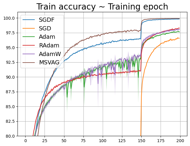
(a) VGG11 on Cifar10

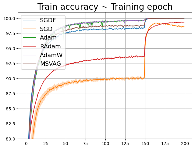
(b) ResNet34 on Cifar10

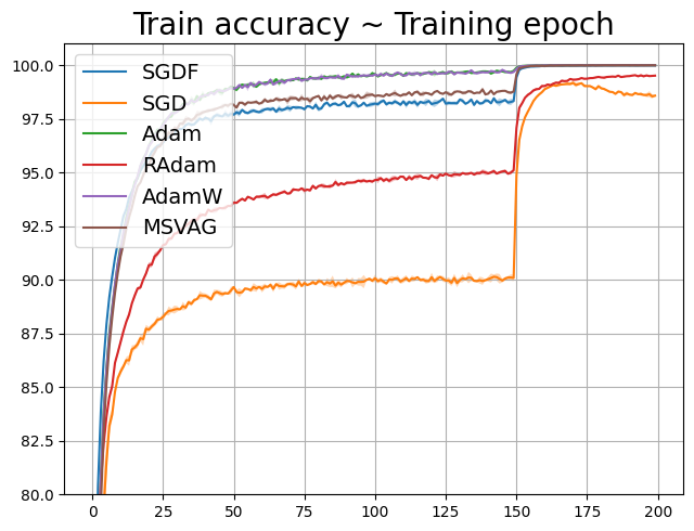
(c) DenseNet121 on Cifar10

(d) VGG11 on Cifar10

(e) ResNet34 on Cifar10

(f) DenseNet121 on Cifar10

Figure 5: Training (top row) and test (bottom row) accuracy of CNNs on Cifar10 dataset. We report confidence interval ([$\mu\pm\sigma$]) of 3 independent runs.

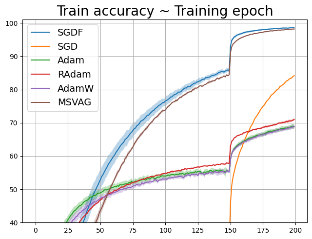
(a) VGG11 on Cifar100

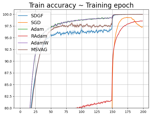
(b) ResNet34 on Cifar100

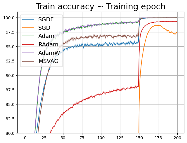
(c) DenseNet121 on Cifar100

(d) VGG11 on Cifar100

(e) ResNet34 on Cifar100

(f) DenseNet121 on Cifar100

Figure 6: Training (top row) and test (bottom row) accuracy of CNNs on Cifar100 dataset. We report confidence interval ([$\mu\pm\sigma$]) of 3 independent runs.

2. Image Classification on ImageNet

We experimented with a ResNet18 on ImageNet classication task. For SGD, we set initial learning rate of 0.1, and multiplied by 0.1 every 30 epochs; for SGDF, we use an initial learning rate of 0.5, set $\beta_{1}$ = 0.5. Weight decay is set as $10^{-4}$ for both cases. To match the settings in (Liu et al., 2019). As shown in Fig. 7, SGDF achieves an accuracy very close to SGD.

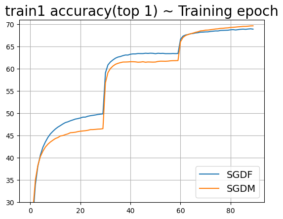
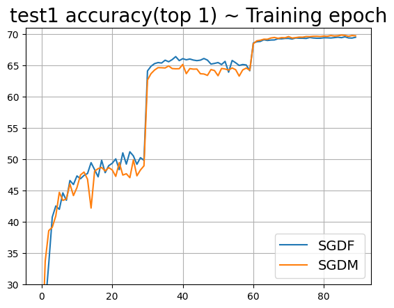
Figure 7: Training and test accuracy (top-1) of ResNet18 on ImageNet.

3. Objective Detection on PASCAL VOC

We show the results on PASCAL VOC(Everingham et al., 2010). Object deetection with a Faster-RCNN model(Ren et al., 2015). The results are reported in Tab. 2, and detection examples shown in Fig. 8. These results also illustrates that our method is still efficient in object detection tasks.

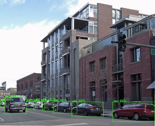
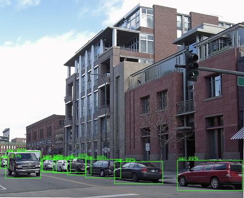
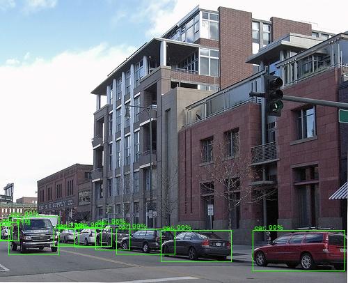
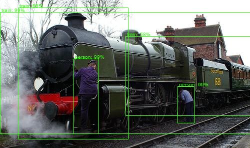
(a) SGDF

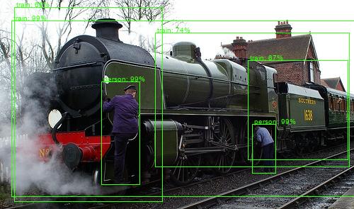
(b) SGDM

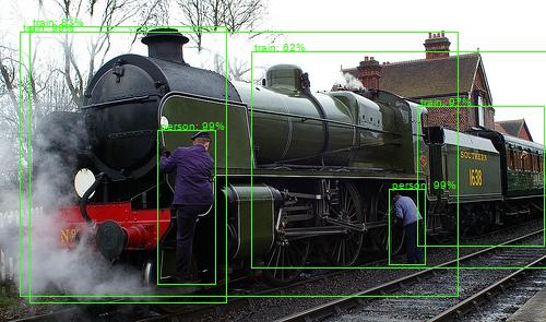
(c) Adam

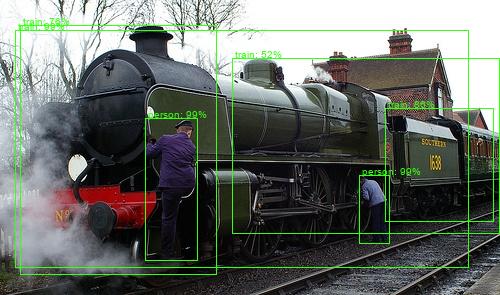
(d) AdamW

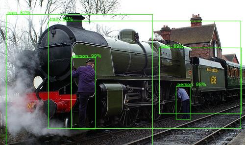
(e) RAdam

Figure 8: Detection examples using Faster-RCNN + FPN trained on PASCAL VOC.

4. Extended Experiment.

The study involves evaluating the vanilla Adam optimization algorithm and its enhancement with a Wiener filter on the Cifar100 dataset. Fig. 9 contains detailed test accuracy curves for both methods across different model. The results indicate that the adaptive learning rate algorithms exhibit improved performance when supplemented with the proposed first moment filter estimation. This suggests that integrating a Wiener filter with the Adam optimizer may lead to better performance.

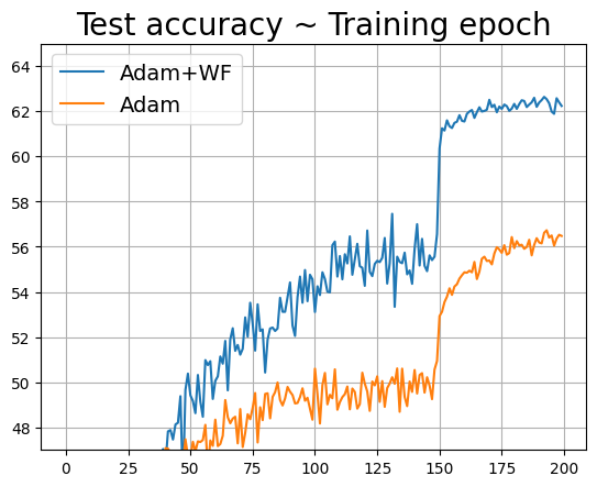
(a) VGG11 on Cifar100

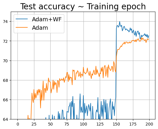
(b) ResNet34 on Cifar100

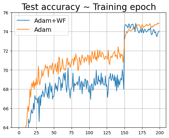
(c) DenseNet121 on Cifar100

Figure 9: Test accuracy of CNNs on Cifar100 dataset. We train vanilla Adam and Adam combined with Wiener Filter.

References

- Arjovsky et al. (2017) Arjovsky, M., Chintala, S., and Bottou, L. Wasserstein gan. 2017.
- Balles & Hennig (2018) Balles, L. and Hennig, P. Dissecting adam: The sign, magnitude and variance of stochastic gradients. In International Conference on Machine Learning, pp. 404–413. PMLR, 2018.
- Bengio & Lecun (2007) Bengio, Y. and Lecun, Y. Scaling learning algorithms towards ai. 2007.
- Bernstein et al. (2020) Bernstein, J., Vahdat, A., Yue, Y., and Liu, M.-Y. On the distance between two neural networks and the stability of learning. Advances in Neural Information Processing Systems, 33:21370–21381, 2020.
- Bottou et al. (2018) Bottou, L., Curtis, F. E., and Nocedal, J. Optimization methods for large-scale machine learning. SIAM review, 60(2):223–311, 2018.
- Caldarola et al. (2022) Caldarola, D., Caputo, B., and Ciccone, M. Improving generalization in federated learning by seeking flat minima. ArXiv, 2022.
- Chandramoorthy et al. (2022) Chandramoorthy, N., Loukas, A., Gatmiry, K., and Jegelka, S. On the generalization of learning algorithms that do not converge. Advances in Neural Information Processing Systems, 35:34241–34257, 2022.
- Chen et al. (2018) Chen, J., Zhou, D., Tang, Y., Yang, Z., Cao, Y., and Gu, Q. Closing the generalization gap of adaptive gradient methods in training deep neural networks. arXiv preprint arXiv:1806.06763, 2018.
- Chen et al. (2023) Chen, X., Liang, C., Huang, D., Real, E., Wang, K., Liu, Y., Pham, H., Dong, X., Luong, T., Hsieh, C.-J., et al. Symbolic discovery of optimization algorithms. arXiv preprint arXiv:2302.06675, 2023.
- Dauphin et al. (2014) Dauphin, Y., Pascanu, R., Gulcehre, C., Cho, K., Ganguli, S., and Bengio, Y. Identifying and attacking the saddle point problem in high-dimensional non-convex optimization. MIT Press, 2014.
- Davtyan et al. (2022) Davtyan, A., Sameni, S., Cerkezi, L., Meishvili, G., Bielski, A., and Favaro, P. Koala: A kalman optimization algorithm with loss adaptivity. In Proceedings of the AAAI Conference on Artificial Intelligence, volume 36, pp. 6471–6479, 2022.
- Defazio et al. (2014) Defazio, A., Bach, F., and Lacoste-Julien, S. Saga: A fast incremental gradient method with support for non-strongly convex composite objectives. In Advances in Neural Information Processing Systems, pp. 1646–1654, 2014.
- Deng et al. (2009) Deng, J., Dong, W., Socher, R., Li, L.-J., Li, K., and Fei-Fei, L. Imagenet: A large-scale hierarchical image database. In IEEE Conference on Computer Vision and Pattern Recognition, 2009.
- Dozat (2016) Dozat, T. Incorporating nesterov momentum into adam. ICLR Workshop, 2016.
- Du & Lee (2018) Du, S. S. and Lee, J. D. On the power of over-parametrization in neural networks with quadratic activation. 2018.
- Duchi et al. (2011) Duchi, John, Hazan, Elad, Singer, and Yoram. Adaptive subgradient methods for online learning and stochastic optimization. Journal of Machine Learning Research, 2011.
- Everingham et al. (2010) Everingham, M., Van Gool, L., Williams, C. K., Winn, J., and Zisserman, A. The pascal visual object classes (voc) challenge. International journal of computer vision, 88(2):303–338, 2010.
- Foret et al. (2021) Foret, P. et al. Sharpness-aware minimization for efficiently improving generalization. In ICLR, 2021. spotlight.
- Geman et al. (2014) Geman, S., Bienenstock, E., and Doursat, R. Neural networks and the bias/variance dilemma. Neural Computation, 4(1):1–58, 2014.
- Goodfellow et al. (2016) Goodfellow, I., Bengio, Y., and Courville, A. Deep learning. MIT Press, 2016.
- Hardt et al. (2015) Hardt, M., Recht, B., and Singer, Y. Train faster, generalize better: Stability of stochastic gradient descent. Mathematics, 2015.
- He et al. (2016) He, K., Zhang, X., Ren, S., and Sun, J. Deep residual learning for image recognition. In Proceedings of the IEEE conference on computer vision and pattern recognition, pp. 770–778, 2016.
- Heusel et al. (2017) Heusel, M., Ramsauer, H., Unterthiner, T., Nessler, B., Klambauer, G., and Hochreiter, S. Gans trained by a two time-scale update rule converge to a nash equilibrium. 2017.
- Hinton (2012) Hinton, G. Neural networks for machine learning. Coursera video lectures, 2012. URL https://www.coursera.org/learn/neural-networks. Lecture 6.5 - rmsprop: Divide the gradient by a running average of its recent magnitude.
- Huang et al. (2017) Huang, G., Liu, Z., Van Der Maaten, L., and Weinberger, K. Q. Densely connected convolutional networks. In Proceedings of the IEEE conference on computer vision and pattern recognition, pp. 4700–4708, 2017.
- Johnson & Zhang (2013) Johnson, R. and Zhang, T. Accelerating stochastic gradient descent using predictive variance reduction. Advances in neural information processing systems, 26, 2013.
- Kalman (1960) Kalman, R. E. A new approach to linear filtering and prediction problems. Journal of Basic Engineering, 1960.
- Kay (1993) Kay, S. M. Fundamentals of Statistical Signal Processing: Estimation Theory, volume 1. Prentice-Hall, Inc., 1993.
- Keskar et al. (2016) Keskar, N. S., Mudigere, D., Nocedal, J., Smelyanskiy, M., and Tang, P. T. P. On large-batch training for deep learning: Generalization gap and sharp minima. 2016.
- Keskar et al. (2017) Keskar, N. S. et al. On large-batch training for deep learning: Generalization gap and sharp minima. In ICLR, 2017.
- Kingma & Ba (2014) Kingma, D. P. and Ba, J. Adam: A method for stochastic optimization. arXiv preprint arXiv:1412.6980, 2014.
- Krizhevsky et al. (2009) Krizhevsky, A., Hinton, G., et al. Learning multiple layers of features from tiny images. 2009.
- Lin et al. (2014) Lin, T.-Y., Maire, M., Belongie, S., Hays, J., Perona, P., Ramanan, D., Dollár, P., and Zitnick, C. L. Microsoft coco: Common objects in context. European Conference on Computer Vision (ECCV), 2014.
- Liu et al. (2023) Liu, H., Li, Z., Hall, D., Liang, P., and Ma, T. Sophia: A scalable stochastic second-order optimizer for language model pre-training. arXiv preprint arXiv:2305.14342, 2023.
- Liu et al. (2019) Liu, L., Jiang, H., He, P., Chen, W., Liu, X., Gao, J., and Han, J. On the variance of the adaptive learning rate and beyond. arXiv preprint arXiv:1908.03265, 2019.
- Loshchilov & Hutter (2017) Loshchilov, I. and Hutter, F. Decoupled weight decay regularization. arXiv preprint arXiv:1711.05101, 2017.
- Lucchi et al. (2022) Lucchi, A., Proske, F., Orvieto, A., Bach, F., and Kersting, H. On the theoretical properties of noise correlation in stochastic optimization. Advances in Neural Information Processing Systems, 35:14261–14273, 2022.
- Luo et al. (2019) Luo, L., Xiong, Y., Liu, Y., and Sun, X. Adaptive gradient methods with dynamic bound of learning rate. arXiv preprint arXiv:1902.09843, 2019.
- Monro (1951) Monro, R. S. a stochastic approximation method. Annals of Mathematical Statistics, 22(3):400–407, 1951.
- Ollivier (2019) Ollivier, Y. The extended kalman filter is a natural gradient descent in trajectory space. arXiv: Optimization and Control, 2019.
- Reddi et al. (2019) Reddi, S. J., Kale, S., and Kumar, S. On the convergence of adam and beyond. 2019.
- Ren et al. (2015) Ren, S., He, K., Girshick, R., and Sun, J. Faster r-cnn: Towards real-time object detection with region proposal networks. Neural Information Processing Systems (NIPS), 2015.
- Ruder (2016) Ruder, S. An overview of gradient descent optimization algorithms. 2016.
- Salimans et al. (2016) Salimans, T., Goodfellow, I., Zaremba, W., Cheung, V., Radford, A., and Chen, X. Improved techniques for training gans. Advances in neural information processing systems, 29, 2016.
- Schmidt et al. (2017) Schmidt, M., Roux, N. L., and Bach, F. Minimizing finite sums with the stochastic average gradient. Mathematical Programming, 162(1):83–112, 2017.
- Simonyan & Zisserman (2014) Simonyan, K. and Zisserman, A. Very deep convolutional networks for large-scale image recognition. Computer Science, 2014.
- Sutskever et al. (2013) Sutskever, I., Martens, J., Dahl, G., and Hinton, G. On the importance of initialization and momentum in deep learning. In International conference on machine learning, pp. 1139–1147. PMLR, 2013.
- Vuckovic (2018) Vuckovic, J. Kalman gradient descent: Adaptive variance reduction in stochastic optimization. ArXiv, 2018.
- Wang et al. (2022) Wang, B., Zhang, Y., Zhang, H., Meng, Q., Ma, Z.-M., Liu, T.-Y., and Chen, W. Provable adaptivity in adam. arXiv preprint arXiv:2208.09900, 2022.
- Wiener (1950) Wiener, N. The extrapolation, interpolation and smoothing of stationary time series, with engineering applications. Journal of the Royal Statistical Society Series A (General), 1950.
- Wilson et al. (2017) Wilson, A. C., Roelofs, R., Stern, M., Srebro, N., and Recht, B. The marginal value of adaptive gradient methods in machine learning. 2017.
- Xie et al. (2020) Xie, Z., Wang, X., Zhang, H., Sato, I., and Sugiyama, M. Adai: Separating the effects of adaptive learning rate and momentum inertia. arXiv preprint arXiv:2006.15815, 2020.
- Xie et al. (2022) Xie, Z., Tang, Q. Y., Cai, Y., Sun, M., and Li, P. On the power-law spectrum in deep learning: A bridge to protein science. 2022.
- Xiong et al. (2020) Xiong, R., Yang, Y., He, D., Zheng, K., Zheng, S., Xing, C., Zhang, H., Lan, Y., Wang, L., and Liu, T. On layer normalization in the transformer architecture. In International Conference on Machine Learning, pp. 10524–10533. PMLR, 2020.
- Yang et al. (2022) Yang, N., Tang, C., and Tu, Y. Stochastic gradient descent introduces an effective landscape-dependent regularization favoring flat solutions. Physical review letters, 2022.
- Yang et al. (2023) Yang, N., Tang, C., and Tu, Y. Stochastic gradient descent introduces an effective landscape-dependent regularization favoring flat solutions. Physical Review Letters, 130(23):237101, 2023.
- Yao et al. (2018) Yao, Z., Gholami, A., Lei, Q., Keutzer, K., and Mahoney, M. W. Hessian-based analysis of large batch training and robustness to adversaries. 2018.
- Yao et al. (2020a) Yao, Z., Gholami, A., Keutzer, K., and Mahoney, M. W. Pyhessian: Neural networks through the lens of the hessian. In International Conference on Big Data, 2020a.
- Yao et al. (2020b) Yao, Z., Gholami, A., Shen, S., Keutzer, K., and Mahoney, M. W. Adahessian: An adaptive second order optimizer for machine learning. arXiv preprint arXiv:2006.00719, 2020b.
- Zaheer et al. (2018) Zaheer, M., Reddi, S., Sachan, D., Kale, S., and Kumar, S. Adaptive methods for nonconvex optimization. Advances in neural information processing systems, 31, 2018.
- Zeiler (2012) Zeiler, M. D. Adadelta: An adaptive learning rate method. arXiv e-prints, 2012.
- Zhang et al. (2016) Zhang, C., Bengio, S., Hardt, M., Recht, B., and Vinyals, O. Understanding deep learning requires rethinking generalization. 2016.
- Zhang et al. (2019) Zhang, J., He, T., Sra, S., and Jadbabaie, A. Why gradient clipping accelerates training: A theoretical justification for adaptivity. arXiv preprint arXiv:1905.11881, 2019.
- Zhang et al. (2023) Zhang, X., Xu, R., Yu, H., Zou, H., and Cui, P. Gradient norm aware minimization seeks first-order flatness and improves generalization. IEEE/CVF Conference on Computer Vision and Pattern Recognition (CVPR), 2023.
- Zhuang et al. (2020) Zhuang, J., Tang, T., Ding, Y., Tatikonda, S. C., Dvornek, N., Papademetris, X., and Duncan, J. Adabelief optimizer: Adapting stepsizes by the belief in observed gradients. Advances in neural information processing systems, 33:18795–18806, 2020.