MirrorCalib: Utilizing Human Pose Information for Mirror-based Virtual Camera Calibration

Abstract

In this paper, we present the novel task of estimating the extrinsic parameters of a virtual camera relative to a real camera in exercise videos with a mirror. This task poses a significant challenge in scenarios where the views from the real and mirrored cameras have no overlap or share salient features. To address this issue, prior knowledge of a human body and 2D joint locations are utilized to estimate the camera extrinsic parameters when a person is in front of a mirror. We devise a modified eight-point algorithm to obtain an initial estimation from 2D joint locations. The 2D joint locations are then refined subject to human body constraints. Finally, a RANSAC algorithm is employed to remove outliers by comparing their epipolar distances to a predetermined threshold. MirrorCalib is evaluated on both synthetic and real datasets and achieves a rotation error of 0.62°/1.82° and a translation error of 37.33/69.51 mm on the synthetic/real dataset, which outperforms the state-of-art method.

I Introduction

To improve health, online coaching and offline learning by watching exercise tutorials are prevalent in daily life. In these tutorials, instructors usually guide students by demonstrating actions in front of a flat mirror in a gym or dance studio. By incorporating a mirrored view of an instructor, both the learning and teaching experience could be enhanced. Especially, instructors can observe and adjust their actions by directly looking at the mirror.

Estimating 3D human motion in exercise videos is crucial to many applications including but not limited to the assessment of trainee exercise quality [36], virtual or augmented reality [37], and motion captioning [38, 39]. However, reconstructing 3D human motion from monocular 2D video input is an ill-posed problem, due to depth ambiguity. The inclusion of mirror view in exercise videos (e.g., Figure 1) provides an additional perspective for the instructors. If the geometric relationship between the real view and the virtual view can be established, in principle, it becomes feasible to determine 3D joint positions through triangulation.

The procedure for establishing the relationship between two camera views is referred to as camera extrinsic parameter estimation or calibration [40]. Extrinsic parameters describe the relative orientation and translation of the camera with respect to a reference frame. Conventionally, the first step in the calibration process involves feature matching of images taken by two cameras. This process includes the detection and association of projections corresponding to the same set of visible features. Feature matching requires an overlapping view of two cameras, which is generally satisfied in stereo systems when the relative rotation between two cameras is small. However, when cameras have little overlapping view (wide baseline) such as a catadioptric system with one real camera and a single mirror (called virtual camera) in coaching videos, feature correspondences are difficult to establish. Even if there exist overlapping views, feature-matching algorithms often fail when the features have complex structures or exhibit repetitive patterns, such as floor or wall tiles [41].

Fortunately, it is possible to leverage “invisible” features that consistently exist in coaching videos. In coaching videos, an instructor is almost always present in both real and virtual views. Consequently, the joints of the instructor can be exploited as feature correspondences for camera calibration in this context. However, 2D human joint locations detected by the state-of-the-art estimators such as OpenPose [25] and HRNet [18] are known to be noisy because of occlusion, inconsistent labeling of training data, unbalanced data, etc [32, 33]. For instance, it was reported that OpenPose has a 75.6% mean Average Precision (mAP) on MPII dataset [34] and 65.3% mean average precision over 10 OKS thresholds on COCO validation set [35]. Naïve structure-from-motion methods to recover the virtual camera pose all suffer from large estimation noise [17]. One key insight is that prior knowledge of human anatomy and motion can be utilized to improve the accuracy of the joint position estimations and thus result in more accurate virtual camera calibration.

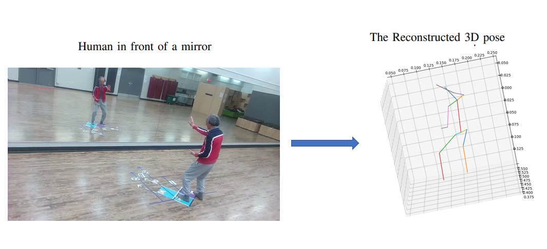
Figure 1: Given images of an individual in front of a mirror, after extrinsic parameter calibration of the virtual camera with respect to a real camera, we can reconstruct the 3D human pose.

Based on the insight, we propose MirrorCalib, a novel pipeline for estimating the extrinsic parameters of a virtual camera (mirror) relative to a real camera in pre-recorded or streaming exercise videos. MirrorCalib consists of three components as illustrated in Figure 2. First, a modified eight-point algorithm with mirror constraints is devised to get the initial camera extrinsic parameters from 2D human joint locations in a sequence of video frames. Next, the 2D joint locations are refined through optimization using characteristics of the human body. After optimization, outlier 2D joint locations are disregarded if their epipolar distances exceed a predefined threshold using random sample consensus (RANSAC). Finally, the extrinsic parameters of the virtual camera with respect to a real camera are calculated from all inliers using the modified eight-point algorithm. The proposed optimization framework and the RANSAC algorithm can be generalized to multi-view setups with real cameras or mirrors.

MirrorCalib has been validated on both synthetic datasets and real datasets. It outperforms the existing methods in the literature which also use 2D human joint locations to calibrate extrinsic parameters in a general multi-view camera setup. Specifically, when intrinsic parameters are known, MirrorCalib achieves a rotation error of 0.62° and a translation error of 37.33 mm on the synthetic dataset and a rotation error of 1.82° and a translation error of 69.51 mm on the real dataset. We have also demonstrated the application of MirrorCalib in 3D human pose estimation with mirrored view and found MirrorCalib contributes to two-third reduction in 3D joint location errors compared to a baseline method that does not perform optimization and outlier removal.

Compared to existing work that calibrates virtual cameras[6, 7, 8, 9], our work differs in two key aspects. First, previous studies[6, 7, 8, 9] often calibrate virtual cameras in catadioptric stereo systems using multiple mirrors. Such systems are not common in daily use. In contrast, MirrorCalib only requires the view of one fixed mirror, which is widely available in gyms and dance studios. Second, since earlier work considers scenarios with more than one mirror, it is easier to obtain overlapping views and rely on visible points to establish correspondences. In contrast, our work utilizes (generally invisible) 2D human joint locations as feature correspondences.

The rest of the paper is organized as follows: a brief review of related work in the literature is provided in Section II, followed by a presentation of the necessary background for our approach in Section III. In Section IV, a detailed explanation of MirrorCalib is provided. Experiment setup, datasets and evaluation results are presented in Section V followed by conclusion in Section VI.

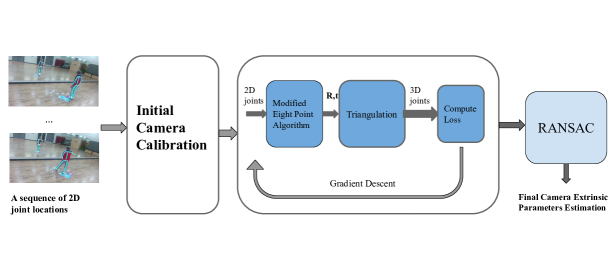
Figure 2: Overview of MirrorCalib. The process takes a video of a human in front of a mirror and passes it through a 2D human pose estimator to obtain the 2D joint locations for both the real and mirrored human. Using a modified eight-point algorithm, an initial estimation of the virtual camera pose is obtained. This estimation is then refined through an optimization process, and a RANSAC algorithm is used to choose the best estimation among all available results.

II Related Work

II-A Camera Calibration with Mirrors

Using mirrors to obtain an additional perspective of objects has been exploited in the literature. This approach is applied in estimating camera pose with respect to an object that is not directly visible to the camera and in 3D reconstruction.

In extrinsic camera calibration, incorporating mirrors provides a viable solution when reference objects are outside the camera FOV. For example, Sturm et al. [26] first estimate the virtual camera pose and mirror planes, and then the real camera pose can be obtained by reflecting the virtual view. They find that the planar motion between pairs of virtual views can be regarded as a fixed-axis rotation and the rotation axis can be estimated. All mirror planes should contain this rotation axis and their positions are determined by the rotation axis and the angle between pairs of virtual views. They also demonstrate that a minimum of three virtual views are needed to determine the positions of mirrors and camera poses. Similarly, Rodrigues et al. [1] estimate the pose of a real camera using a minimum of three virtual views and by employing knowledge of fixed-axis rotations. However, their approach differs in computing the mirror direction in a single step without relying on the inference from the axis angle. Without using fixed-axis rotation as constraints, Kumar et al. [3] find out that for each column vector of the rotation matrix of the real camera, the summation of the vector with the corresponding column vector of the rotation matrix of its mirrored camera is orthogonal to the vector connecting a real camera and its mirrored camera. They apply this constraint to solve the real camera pose but require at least five mirrored images. Long et al. [4] also provide a solution that does not rely on the fixed-axis rotation constraint. They formulate the rotation of the real camera and the rotation of its mirrored camera as a rotation averaging problem and solve it using an optimization framework. All the aforementioned methods do not consider the number of known 3D reference points. In case where the number is three, there can be up to four possible solutions for extrinsic parameters. If 3 mirrored images are utilized to recover the real camera pose, 64 = $4\crossproduct 4\crossproduct 4$ combinations of 3D reference points are possible. Takahashi et al. [2] propose an orthogonality constraint to choose the best combination of reference points without explicitly computing the corresponding extrinsic parameters. Instead of planar mirrors, Agrawal and Ramalingam [5] utilize spherical mirrors in their approach to avoid the problem of parallel mirrors configuration. However, planar mirrors are still more common in practice, and our paper only considers planar mirrors.

Catadioptric stereo systems, leveraging multiple mirrors for additional views, have also been applied in 3D reconstruction. This task is close to our scenario. However, the extrinsic parameters of a virtual camera are usually calibrated relative to another virtual camera. Some authors use a single perspective camera and two planar mirrors to build a stereo system [6, 7, 8, 9]. Those works calibrate the virtual cameras using image correspondences like general structure-from-motion methods. After the derivation of epipolar geometry based on mirror constraints, the number of unknown extrinsic calibration parameters can be reduced. In this work, we use 2D human joint correspondences to calculate the extrinsic parameters of the virtual camera with respect to a real camera.

To the best of our knowledge, our paper is the first work that considers calibrating the virtual camera with respect to a real camera in a catadioptric stereo system with only one fixed planar mirror. In contrast, existing methods targeting catadioptric stereo systems either require a mirror to be moved to multiple positions or involve multiple mirrors to obtain overlapping views.

II-B Extrinsic Camera Calibration with Human Pose Information

Prevailing methods of camera calibration utilize chessboard corners or local features like SIFT as corresponding points to recover relative camera poses. When the cameras have little overlapping views (wide baselines), image feature correspondences are difficult to establish. Incorrect feature correspondences can severely degrade camera calibration results. Therefore, methods have been proposed to utilize prior knowledge of humans to calibrate cameras. The studies in [14, 15] use the silhouettes of humans to establish the corresponding points. With the advances in 2D human pose estimation from single images, Puwein et al. [11] propose the first method to use detected 2D human joints in multi-view images as feature points to calculate the extrinsic parameters of the respective cameras. After initial calibration, with the initial 3D joint positions obtained through triangulation, the camera parameters and 3D human poses are further optimized by the application of constraints on smooth motion, ensuring the consistency of detected poses with optical flow, and taking into account the discriminative scores of 2D joints. Similarly, Takahashi et al. [12] present an approach that utilizes a relaxed reprojection error in robust optimization. As most 2D pose estimators produce a confidence map for each joint, the reprojection error is small when the reprojected point is in an area of high confidence. Huang et al. [13] design a VAE-based latent motion prior to jointly optimizing extrinsic parameters and human motion. All of these works use noisy 2D joint estimation to compute initial camera extrinsic parameters and 3D joint positions, and then refine the parameters and human joint positions together through an optimization process.

This work focuses on calibrating virtual camera parameters relative to a real camera, which differs from multi-view camera calibration. Conceptually, methods in [11, 12, 13] can be applied to our problem setting as well. However, the direct application of these methods fails to exploit the geometry constraints imposed by mirrors that can reduce the number of unknowns in the calculation of the fundamental matrix. Moreover, a RANSAC algorithm that leverages epipolar distances to identify the inliers is applied in MirrorCalib.

III Background

In this section, key geometric concepts relevant to estimating virtual camera poses with respect to a real camera are provided and the general normalized eight-point algorithm for fundamental matrix calculation is introduced. It serves as the basis for the proposed eight-point algorithm with mirror constraints in the Methodology section.

III-A Planar Mirror Reflection Geometry

In this paper, we treat the real camera frame as the coordinate system where the optical center of the real camera is the origin. Let the intrinsic parameter matrix of the camera be $\mathbf{K}$. We consider the configuration depicted in Figure 3, in which a perspective camera $C$ is in front of a planar mirror $\pi$ that is uniquely defined by its normal vector $\mathbf{n}$ and a distance $d$ to $C$. Any point $x$ on $C$’s image plane satisfies the condition that $\mathbf{n}^{T}x=d$. The symmetric transformation between a point $p$ and its mirrored point $p^{\prime}$ with respect to $\pi$ is given by:

$$\begin{bmatrix}p^{\prime}\\ 1\end{bmatrix}=S\begin{bmatrix}p\\ 1\end{bmatrix},\quad\text{where}\quad S=\begin{bmatrix}\mathbf{I}-2\mathbf{nn}^{T}&2d\mathbf{n}\\ \bm{0}&1\end{bmatrix}$$ (1)

Denote by $\tilde{\mathbf{u}}$ and $\tilde{\mathbf{u}}^{\prime}$ the homogeneous coordinates of the point $p$ and the point $p^{\prime}$ projected onto the image planes of the real camera $C$. Since the projection $\tilde{\mathbf{u}}$ of $p$ is given by:

$$\alpha\tilde{\mathbf{u}}=\mathbf{K}\begin{bmatrix}\mathbf{I}&\bm{0}\end{bmatrix}\begin{bmatrix}p\\ 1\end{bmatrix}\quad\text{where }\alpha\in\mathbb{R}^{+}\text{is a scale parameter},$$ (2)

the projection $\mathbf{u^{\prime}}$ of the mirrored point $p^{\prime}$ is:

$$\alpha\tilde{\mathbf{u}}^{\prime}=\mathbf{K}\mathbf{S}\begin{bmatrix}\mathbf{I}&\bm{0}\end{bmatrix}\begin{bmatrix}p\\ 1\end{bmatrix}\text{ }\text{where }\alpha\in\mathbb{R}^{+}\text{is a scale parameter}.$$ (3)

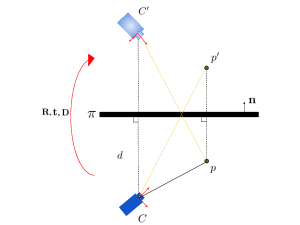
Figure 3: The coordinates frame of real and virtual cameras and their relationship. $\mathbf{R}$, $\mathbf{t}$, $\mathbf{D}$ are rotation, translation and reflection transformation respectively.

III-B Virtual Camera Projection with Reflective Surfaces and Reflective Epipolar Geometry

The projection $\mathbf{u^{\prime}}$ of the mirrored point $p^{\prime}$ can be seen as the projection $\mathbf{u}^{\prime\prime}$ of the point $p$ on the image plane of a virtual camera $C^{\prime}$. The reference frame of the virtual camera is obtained by reflecting that of the real camera about the mirror $\pi$. It should be noted that the real camera is right-handed i.e., the orientation of the camera’s coordinate system follows the right-hand rule, while the virtual camera is left-handed. As shown in Figure 3, the projection of point $p^{\prime}$ on $C$ is the same as the projection of $p$ onto the image plane of $C’$. Since both the real camera and its virtual counterpart share the same set of intrinsic parameters, the purpose of camera calibration in this context is to estimate the extrinsic parameters between these two camera frames, specifically, the rotation matrix $\mathbf{R}$ and the translation vector $\mathbf{t}$.

From [16], $\tilde{\mathbf{u}}$ and $\tilde{\mathbf{u}}^{\prime}$ satisfy the reflective epipolar constraint:

$$(\tilde{\mathbf{u}}^{\prime})^{T}\mathbf{F}\tilde{\mathbf{u}}=0,$$ (4)

where

$$\mathbf{F}\triangleq\mathbf{K}^{-T}\mathbf{E}\mathbf{K}^{-1}$$ (5)

is the reflective fundamental matrix, and

$$\mathbf{E}=2d[\mathbf{n}]_{\times}$$ (6)

is the reflective essential matrix, where $[\mathbf{n}]_{\times}$ is the skew-symmetric matrix associated with the normal vector $\mathbf{n}$. Note that since the reflective essential matrix is a skew-symmetric matrix, after transformation by the intrinsic camera matrix, the reflective fundamental matrix is also a skew-symmetric matrix.

III-C General Normalized Eight-Point Algorithm

The projections of a point onto the image planes of two cameras related by a fundamental matrix $F$ satisfy Equation (4). For every matched pair $\tilde{\mathbf{u}}=[u,v,1]^{T}$, $\tilde{\mathbf{u}}^{\prime}=[u^{\prime},v^{\prime},1]^{T}$, we have a linear equation of unknown entries in fundamental matrix $\mathbf{F}$. If we denote a row vector $[uu^{\prime},uv^{\prime},u,vu^{\prime},vv^{\prime},v,u^{\prime},v^{\prime},1]^{T}$ by $\mathbf{a}$ and stack all entries of $\mathbf{F}$ in a row-major order to a vector $\mathbf{f}$, Equation (4) is equivalent to $\mathbf{a^{T}f}=0$. Given multiple pairs of ($\tilde{\mathbf{u}}$, $\tilde{\mathbf{u}}^{\prime}$), the system of equations is given by:

$$\mathbf{Af}=\mathbf{0},\text{ }\mathbf{||f||}=1.$$ (7)

Since the rank of $\mathbf{A}$ is eight [17], a solution can be found with eight matched non-coplanar pairs. When the number of matched pairs exceeds eight, Equation (7) is over-determined. Furthermore, real-world data often contain noise, which may result in infeasibility. Therefore, a least-square optimization can be formulated to minimize the $L_{2}$ norm of $\mathbf{Af}$. The solution to the optimization problem can mitigate the effects of noise and improve the accuracy of the estimation.

Directly applying the classic eight-point algorithm to compute the fundamental matrix is known to be highly sensitive to noise. In [17], it is shown that normalizing the coordinates of the matched points $\tilde{\mathbf{u}}_{i}^{\prime}=[u^{\prime}_{i},v^{\prime}_{i},1]$ and $\tilde{\mathbf{u}}_{i}=[u_{i},v_{i},1]$ can improve noise robustness. Specifically, let

$$\hat{\tilde{\mathbf{u}}}^{\prime}=\mathbf{T^{\prime}}\tilde{\mathbf{u}}’$$ (8)

$$\hat{\tilde{\mathbf{u}}}=\mathbf{T}\tilde{\mathbf{u}}$$ (9)

$$\mathbf{T}=\begin{bmatrix}s&0&-st_{x}\\ 0&s&-st_{y}\\ 0&0&1\end{bmatrix},\quad\mathbf{T^{\prime}}=\begin{bmatrix}s^{\prime}&0&-s^{\prime}t_{x}^{\prime}\\ 0&s^{\prime}&-st_{y}^{\prime}\\ 0&0&1\end{bmatrix}.$$ (10)

Then the original fundamental matrix can be computed by:

$$\mathbf{F}=\mathbf{T^{\prime}}^{T}\mathbf{F^{\prime}}\mathbf{T},$$ (11)

where $s$ and $s^{\prime}$ are positive scale factors, $(t_{x},t_{y})$ and $(t_{x}^{\prime},t_{y}^{\prime})$ are coordinates of the centroids of all image points of the real view and its virtual view, and $\mathbf{F}^{\prime}$ is the fundamental matrix for normalized image points, respectively. This normalization brings the centroid of the set of points in each image to the origin and normalizes coordinates such that the average distance of points to the origin is $\sqrt{2}$. Then for normalized eight-point algorithm, each row vector of $\mathbf{A}$ in equation (7) is formed by normalized coordinates $[\hat{u}\hat{u}^{\prime},\hat{u}\hat{v}^{\prime},\hat{u},\hat{v}\hat{u}^{\prime},\hat{v}\hat{v}^{\prime},\hat{v},\hat{u}^{\prime},\hat{v}^{\prime},1]^{T}$. And $\mathbf{F}^{\prime}$ can be solved using a least-square optimization algorithm when the number of matched pairs exceeds eight.

IV Methodology

In this section, we present the detailed procedure of MirrorCalib to determine the reflective fundamental matrix from noisy 2D pose estimations.

IV-A Eight-Point Algorithm for Solving Reflective Fundamental Matrix

Typically a pair of real cameras have nine unknowns in the fundamental matrix. However, in the case of the reflective fundamental matrix between a real camera and its virtual one, as explained in Section III-B, the fundamental matrix is a skew-symmetric matrix determined by only three unknowns. Therefore, the transformed fundamental matrix after image normalization is:

$$\mathbf{F}^{\prime}=\begin{bmatrix}0&x_{1}&x_{2}\\ -x_{1}&0&x_{3}\\ x_{4}&x_{5}&x_{6}\end{bmatrix},$$ (12)

where $[x_{1},x_{2}...x_{6}]$ are unknowns. The fundamental matrix can be solved through least-square minimization. Specifically, the matrix $\mathbf{\hat{A}}$ is obtained by forming a row vector for each pair of matching points $[-\hat{v}^{\prime}\hat{u}+\hat{u}^{\prime}\hat{v},\hat{u}^{\prime},\hat{v}^{\prime},\hat{u},\hat{v},1]$, where $\hat{u}$’s and $\hat{v}$’s are normalized coordinates. The objective is to minimize:

$$\mathbf{\hat{A}}\mathbf{f^{\prime}}\quad\text{s.t. }||\mathbf{f^{\prime}}||=1,$$ (13)

where $\mathbf{f’}$ is the vector $[x_{1},x_{2}...x_{6}]^{T}$ that determines $\mathbf{F}^{\prime}$. The least-square solution to Equation (13) can be calculated by getting the smallest eigenvalue of $\mathbf{A^{T}A}$. After $\mathbf{F^{\prime}}$ is obtained, we transform it to the original reflective fundamental matrix $\mathbf{F}$ by Equation (11).

IV-B Reflective Essential Matrix Decomposition

Different from the multi-view epipolar geometry with real cameras, the reference frame of the virtual camera is left-handed. Thus, we decompose the transformation from a real camera reference frame to that of the virtual camera frame into rotation $\mathbf{R}$, translation $\mathbf{t}$, followed by reflection $\mathbf{D}$, as illustrated in Figure 3. The reflection from the right-handed frame to the left-handed frame can be simply defined as:

$$\mathbf{D}=\begin{bmatrix}-1&0&0\\ 0&1&0\\ 0&0&1\end{bmatrix}.$$ (14)

Therefore, the essential matrix that relates the corresponding points on the image planes of the real and virtual cameras is given by:

$$\mathbf{E}=[\mathbf{t^{\prime}}]_{\times}\mathbf{D}\mathbf{R}\quad\text{where}\quad\mathbf{t^{\prime}}=\mathbf{D}\mathbf{t}.$$ (15)

Similar to a conventional essential matrix, $\mathbf{R}$ and $\mathbf{t}$ can be obtained from the reflective essential matrix $\mathbf{E}$ using singular value decomposition (SVD). Details of the procedure can be found in the Appendix.

IV-C Estimating Virtual Camera Extrinsic Parameters from 2D Human Pose Estimation

Next, we discuss how to utilize 2D joint coordinates from 2D pose estimation to estimate the extrinsic parameters of the virtual camera $C^{\prime}$.

IV-C1 Initial Estimation

Given the video of a human performing actions in front of a mirror, we first apply a state-of-the-art 2D human pose estimator on each frame to get the 2D joint positions of the real human and the mirrored human. The 2D joint locations on each joint are then matched and used in calibration. Special care must be taken, since the joints of the real human and the mirrored human are symmetrically associated. For instance, the right ankle joint of the real human should correspond to the left ankle of the mirrored human. We employ the modified eight-point algorithm in Section IV-A to calculate the reflective fundamental matrix and the reflective essential matrix. Lastly, the reflective essential matrix is used to decompose and calculate the virtual camera pose with respect to the real camera following the procedure in the Appendix.

Not all joints are suitable for estimating the virtual camera extrinsic parameters. We omit the joints on one’s face, feet, and hands because these areas tend to have a lower resolution and are often occluded in the frames.

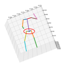
Figure 4: Illustration of hip constraints. The left hip, right hip, and mid-hip keypoints should be co-linear.

IV-C2 Refining 2D Joint Locations

As the key joint positions from 2D human pose estimation tend to be noisy due to occlusion, limited light, and low image resolution, the initial estimates of the extrinsic parameters are inaccurate. To improve their accuracy, we utilize the prior knowledge of the human body. Rather than optimizing the extrinsic parameters directly, we optimize the 2D human joints of the real and virtual human together and use the updated positions to estimate the parameters.

Let $\mathbf{u_{i}^{t}}$ and $\mathbf{{u_{i}}^{t}}^{\prime}$ denote the 2D coordinates of joint $i$ and reflected joint $i^{\prime}$ at time $t$, $\mathbf{\Theta}$ and $\mathbf{\Theta^{\prime}}$ denote the extrinsic parameters of camera $C$ and the virtual camera $C^{\prime}$ respectively where $\mathbf{\Theta}$ is known. $\mathbf{\Theta^{\prime}}$ is updated by the modified eight-point algorithm in each iteration, and $\mathbf{X}_{i}^{t}$ denote the 3D coordinates of joint $i$ at time $t$. $\mathbf{X}_{i}^{t}$ can be calculated through triangulation from $\mathbf{u_{i}^{t}}$, $\mathbf{{u_{i}}^{t}}^{\prime}$, $\mathbf{\Theta}$ and $\mathbf{\Theta^{\prime}}$. Our goal is to “denoise” $\mathbf{u}_{i}^{t}$ and ${\mathbf{u}_{i}}^{t^{\prime}}$, to refine the estimation of $\mathbf{\Theta^{\prime}}$. One body prior is that the length of each limb remains constant over the duration of the recording. Let $l_{k}^{t}$ be the length of the $k_{th}$ bone in the bone set $P$ = {Right Femur, Left Femur, Left Humerus, Right Humerus, Left Ulna, Right Ulna, Left Tibia, Right Tibia, Left Scapular, Right Scaptular, Left Hip, Right Hip} at time $t$ from estimated 2D joint positions. To account for the discrepancies in bone length, we introduce a penalty term that considers the ratio of bone length variation over time to the mean bone length:

$$L_{\text{var}}=\sum_{k\in P}\frac{\Delta l_{k}}{\bar{l_{k}}},$$ (16)

where $\Delta l_{k}$ is the variation of bone length over T frames and $\bar{l_{k}}$ is the mean bone length over T frames.

Let $m(\cdot)$ be an operator that maps the index of a bone to the index of its counterpart on the symmetric side of the body. For example, if $k$ is the index of the right femur, $m(k)$ corresponds to the left femur, and vice versa. Under the assumption that the human body is symmetrical, we define a loss term associated with body symmetry as,

$$L_{\text{sym}}=\sum_{t}^{T}\sum_{k\in P}||l_{k}^{t}-{l_{m(k)}^{t}}||.$$ (17)

Let $\sigma_{k}$ be the average normalized length of bone $k$ among abled-bodied humans without physical deformity (eg. according to the statistics from CAESAR Dataset [21]). Let $\hat{l_{k}^{t}}=\frac{l_{k}^{t}}{l_{femur}^{t}}$, i.e., the length of the $k_{th}$ bone normalized by the length of the longest femur. The loss term associated with anthropometric constraints is thus,

$$L_{\text{anth}}=\sum_{t}^{T}\sum_{k\in P}(\hat{l}_{k}^{t}-\sigma_{k})^{2}.$$ (18)

Let $\mathbf{v_{ml}}^{t}$ ($\mathbf{v_{mr}}^{t}$) be the vectors from the left (right) hip to the mid-hip (Figure 4). It is expected that the left hip, right hip, and mid-hip joints are co-linear. Thus, we define:

$$L_{\text{hip}}=\sum_{t}^{N_{t}}||{\mathbf{v_{ml}}}^{t}\times{\mathbf{v_{mr}}}^{t}||,$$ (19)

to penalize abnormal posture of the hips.

The smoothness of motion is a characteristic of human movement, whereby the change in 3D joint locations between consecutive frames is typically gradual and continuous. Therefore, a loss term associated with the second derivative of 3D joint locations approximated by central finite differences is introduced:

$$L_{\text{smooth}}=\sum_{t}^{N_{t}}\sum_{i\in P}^{N}\mathbf{\ddot{X}_{i}^{t}}.$$ (20)

Lastly, the denoised 2D joint locations should not deviate too much from the initial estimation. The following reprojection term penalizes the deviation from the original posture:

$$L_{\text{repro}}=\sum_{t}^{T}\sum_{i\in P}^{N}\rho(||\Pi(\mathbf{\Theta},\mathbf{X_{i}^{t}})-\mathbf{u_{i}^{t}}||+||\Pi(\mathbf{\Theta^{\prime}},\mathbf{X_{i}^{t}})-\mathbf{{u_{i}}^{t}}^{\prime}||),$$ (21)

where $\Pi$ is the projection operator from 3D to 2D, and $\rho$ denotes the Geman-McClure robust error function to suppress outliers.

To this end, the final objective function can be written by combining Equations (16) to (21) as follows:

$$\underset{\text{{$\mathbf{u,u^{\prime}}$}}}{\text{min}}\quad\lambda_{\text{var}}L_{\text{var}}+\lambda_{\text{sym}}L_{\text{sym}}+\lambda_{\text{anth}}L_{\text{anth}}+\lambda_{\text{hip}}L_{\text{hip}}$$ (22)

$$+\lambda_{\text{smooth}}L_{\text{smooth}}+\lambda_{\text{repro}}L_{\text{repro}},$$

where $\lambda$’s are empirically chosen weights.

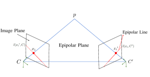
Figure 5: An epipolar plane is created by connecting a point in three-dimensional space to the optical centers of the real and virtual cameras, and this plane intersects with the image plane to form the corresponding epipolar line.

IV-C3 Outlier Rejection

After the optimization in Section IV-C2, “denoised” 2D joint locations in T frames are obtained. There are many more pairs than needed to solve for the fundamental matrix. To further improve the calibration accuracy, we reject outliers by computing the epipolar distances for eligible pairs for a given fundamental matrix $F$. Specifically, given a point in three-dimensional space, an epipolar plane is defined by the intersection of the line connecting the point to the optical centers of two cameras as shown in Figure 5. This epipolar plane intersects the image planes and forms the epipolar lines. Let $l(x_{i},C^{\prime})=\mathbf{F}x_{i}$ and $l(x_{i}^{\prime},C)=\mathbf{F}^{T}{x_{i}}^{\prime}$ be the epipolar lines generated by the 2D point $x_{i}$ on the virtual view $C^{\prime}$ and the matched 2D point ${x_{i}}^{\prime}$ on the real view $C$ respectively. Then we can compute the sum of the distance from ${x_{i}}^{\prime}$ to $l(x_{i},C^{\prime})$ and the distance from $x_{i}$ to $l({x_{i}}^{\prime},C)$ in each frame in a video sequence and denote this sum as $g(\mathbf{F})=distance(l(x_{i},C^{\prime}),x_{i}^{\prime})+distance(l(x_{i}^{\prime},C),x_{i})$.

Next, the Random Sample Consensus (RANSAC) algorithm for outlier removal is applied. Beginning with a set of six pairs of 2D joint positions selected at random, an iterative process is used to calculate the fundamental matrix. This matrix is then used to categorize the pairs into two groups: inliers and outliers, based on their respective epipolar distances. The largest inlier set is used to determine the fundamental matrix as described in Section IV-A. The detailed steps are summarized in Algorithm 1.

Algorithm 1 RANSAC Algorithm for Estimating Fundamental Matrix

1:

2:Corresponding feature points $\{x_{i},x^{\prime}_{i}\}_{i=1}^{n}$

3:The maximum number of iterations $K$

4:inlier threshold $\tau$

5:The minimum number of inliers $\gamma$

6:

7:Fundamental matrix $\mathbf{F}$

8:$itr\leftarrow 0$, $best\_inliers\leftarrow\varnothing$

9:while $itr<K$ and $|best\_inliers|<\gamma$ do

10:     $S\leftarrow$ random sample of 6 pairs of features from $\{x_{i},x^{\prime}_{i}\}_{i=1}^{n}$

11:     $\mathbf{F}\leftarrow$ compute fundamental matrix using $S$

12:     $inliers\leftarrow\varnothing$

13:     for $i=1$ to $n$ do

14:         if $d_{i}(\textbf{F})<\tau$ then

15:              Add $i$ to $inliers$

16:         end if

17:     end for

18:     if $|inliers|>|best\_inliers|$ then

19:         $best\_inliers\leftarrow inliers$

20:     end if

21:     $itr\leftarrow itr+1$

22:end while

23:$\mathbf{F}\leftarrow$ re-estimate fundamental matrix using all points in $best\_inliers$

24:return $\mathbf{F}$

V Evaluation

In this section, we evaluate the performance of MirrorCalib on both synthetic dataset and real datasets. We conduct experiments to demonstrate the influence of the number of frames and the errors in 2D human pose estimation. Since MirrorCalib is dependent on the intrinsic parameters of cameras, the impact of the accuracy of intrinsic parameters is also evaluated. Furthermore, we conduct a case study on 3D HPE to illustrate the practical application of MirrorCalib.

V-A Implementation Details

V-A1 Intrinsic Parameters

MirrorCalib assumes that the intrinsic parameters that characterize the focal length and optical center are given as in previous work [11, 12, 13]. These intrinsic parameters can be obtained from the metadata of videos recorded by professional cameras. Alternatively, they can be estimated using vanishing points [23] under the assumption that the camera has zero skew, square pixels, and the principal point is located at the image center. In the case where no ground-truth intrinsic parameters are available, we introduce additional steps to estimate these parameters in the proposed pipeline (Figure 2) as follows:

1. Use the detected 2D keypoints and mirror edges to estimate the focal length following the method in [23]. Specifically, the pairs of keypoints in the real and mirrored view are used to compute one vanishing points, while the second vanishing point is determined as the intersection of mirror edges from the real view;

2. Incorporate the estimated focal length in the normalized mirror-constrained eight-point algorithm (Section IV-A), to derive the initial set of extrinsic parameters;

3. Refine the extrinsic parameters through optimization, integrating prior knowledge of the human body;

4. Employ the RANSAC algorithm to identify inliers for the re-estimation of extrinsic parameters;

5. Repeat (1) using only the selected inliers and mirror edges;

6. Compute the final set of extrinsic parameters using the updated focal length.

V-A2 2D Human Pose Estimation

In the implementation, we adopt HRNet [18] and OpenPose [25] to estimate the 2D joint locations of the human and the mirrored human frame by frame from a video sequence of a human moving in front of a mirror. The outputs of HRNet consist of 2D joint locations of eyes, ears, nose, shoulders, elbows, wrists, left and right hips, knees, and ankles. The body25 format output of OpenPose consists of 2D joint locations of eyes, ears, nose, shoulders, elbows, wrists, left and right hips, mid-hip, knees, ankles, and joints on the foot. Since HRNet does not provide 2D joint location of the mid-hip, the hip-angle loss is not adopted when HRNet is utilized. The joints except for those on a face and feet are used to obtain an initial estimation of the camera extrinsic parameters.

V-A3 Training

L-BFGS is used in solving the optimization problem in Equation (22). The learning rate of L-BFGS is set to be 1 and the maximum number of iterations in one optimization step equals 20. The pipeline is implemented in Python.

V-B Baseline Methods and Evaluation Metrics

In order to evaluate the effectiveness of MirrorCalib, we compare its performance with two baseline methods. The first baseline method operates on the same collection of frames and employs the normalized eight-point algorithm without mirror constraints, optimization, or RANSAC. The second baseline method combines the modified eight-point algorithm and optimization with the loss terms in a previous study for multi-view cameras [12]. Note that there is no prior work on calibrating the extrinsic parameters of a virtual camera relative to a real camera using 2D human joint locations.

To evaluate the accuracy of virtual camera orientations, we calculate the rotation in the axis-angle representation between the ground truth and estimated rotation matrices. The resulting angle is used as the error metric, expressed in degrees. To calculate the translation errors, we transform the estimated translation vector $\mathbf{t}$ so that it has the same scale as the ground-truth translation vector. Then the difference between the ground-truth $\mathbf{\hat{t}}$ and the scaled translation vectors is the translation error expressed in millimeters (mm). The translation error for each estimation is given by:

$$E_{t}=||\mu\mathbf{t}-\mathbf{\hat{t}}||\quad\text{where }\mu=||\mathbf{\hat{t}}||/||\mathbf{t}||$$ (23)

V-C Datasets

Since there are no existing video datasets with mirrors including ground truth virtual camera parameters, we create a synthetic dataset and collect a real-world dataset.

V-C1 Synthetic Dataset

To create the dataset, we utilize SMPL [19], a differentiable function that produces a human body mesh based on pose and shape parameters. The 3D joint locations can be generated from a linear combination of mesh vertices. We use the SMPL parameters of human motions provided by the SURREAL dataset [27] to obtain the ground-truth 3D body joint locations for the synthetic dataset.

To obtain 2D poses, we project the synthetic 3D body joints onto the image planes of both real and virtual cameras using given intrinsic and extrinsic parameters. These 2D joint locations of the real human and the mirrored human are taken as ground truth. To emulate 2D pose estimation errors, we add Gaussian noise to the ground truth locations and vary its mean and standard deviation. From evaluations using public datasets such as Human3.6 [20] and Mirrored-Human [23], we find the mean and standard deviation errors of state-of-art 2D pose estimators such as HRNet are approximately 0.076 and 4.0 pixels. The resulting noisy 2D joint locations are subsequently used as input to the baseline methods and MirrorCalib. The synthetic dataset allows us to investigate the impact of 2D pose estimation errors and other parameters on different methods in a controlled manner.

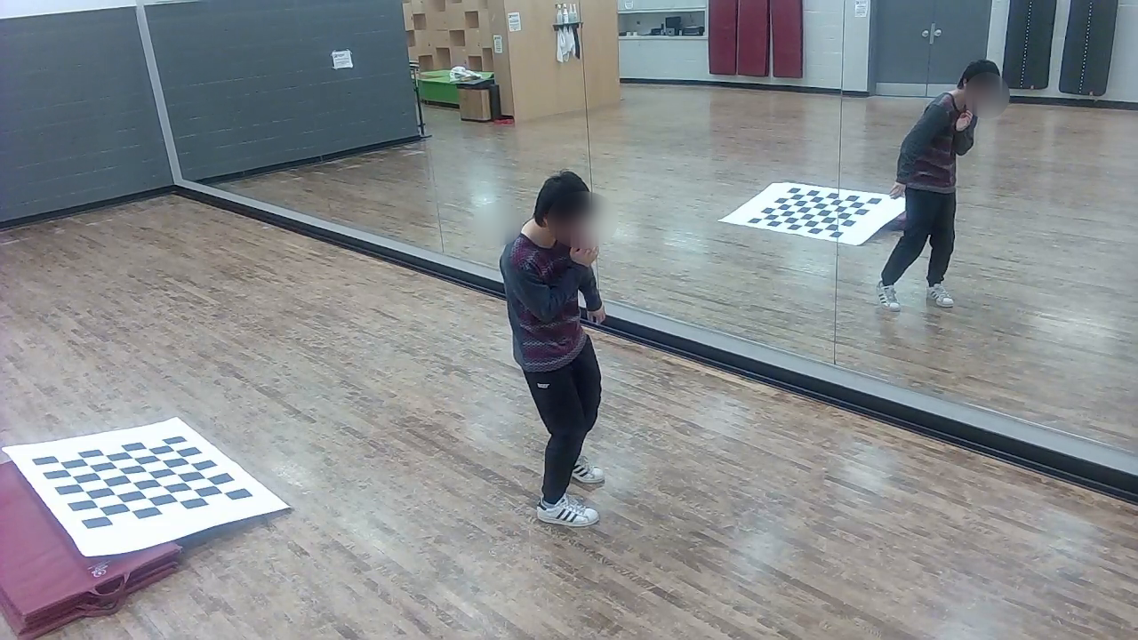
Figure 6: Real dataset collection setup. The chessboard can be captured in both real and virtual views. The corners on the chessboard are only for ground-truth derivation, and are not the key points for MirrorCalib.

V-C2 Real Dataset

We recruited seven subjects (5 males and 2 females) performing various actions in front of a mirror and recorded their movements for five minutes per camera location using the WEBCAM C3 model from ASUS. There are a total of 31 different camera positions for these videos. The resolution of those videos is 1920$\crossproduct$1080 and the frame rate is 30 fps. The intrinsic parameters of the camera are obtained by using a chessboard and an OpenCV toolbox [24]. To obtain the ground-truth extrinsic parameters, we placed a chessboard in front of the mirror, ensuring that the camera captured both its real and virtual views. After associating the corners of the real and mirrored chessboards, the extrinsic parameters of the virtual camera are calculated using the modified eight-point algorithm and are treated as ground truth.

V-D Results on the Synthetic Dataset

V-D1 Impacts of 2D Human Pose Estimation Accuracy

In the first set of experiments, we evaluate the impact of varying errors of 2D human pose estimation on virtual camera extrinsic parameter estimation. In the experiments, the mean error and number of frames (T) are set to be 0.076 pixels and 1000, respectively, but the standard deviation of the errors varies from 1 to 15 pixels. Figure LABEL:extrinsic_experiments shows the rotation and translation errors of extrinsic parameters from different methods. As expected, increasing the standard deviation of 2D human pose estimation leads to larger errors in virtual camera extrinsic parameters in all methods. This underscores the importance of having an accurate 2D human pose estimator.

MirrorCalib outperforms all baseline methods and its performance degrades more gradually as the standard deviation of 2D pose estimation errors increases. When the standard deviation equals 4.0 pixels, the rotation error and translation error of MirrorCalib are 0.62° and 37.3 mm. The inclusion of mirror constraints improves the accuracy of the 8-point algorithm.

V-D2 Impact of the Number of Frames

Next, we assess the impact of T, the number of frames used in virtual camera calibration. The mean and the standard deviation of 2D human pose estimation errors are set to be 0.076 and 4.0 pixels, respectively. As illustrated in Figure LABEL:extrinsic_experiments, increasing the number of frames results in increased accuracy of all methods. However, even when the number of frames is small (e.g., when T = 200), MirrorCalib has achieved a significant reduction in errors. This can be attributed to the ability of the optimization procedure and RANSAC to combat noisy 2D position errors.

V-D3 Ablation Study

We further conduct an ablation study on the synthetic dataset to evaluate the impact of the two pillars of MirrorCalib: optimization and RANSAC. The mean and standard deviation of 2D human pose estimation error are set to be 0.076 and 4.0 pixels respectively and the number of frames equals 1000. The results are summarized in Table I. For comparison, we also include the results of the baseline methods. Table I reveals that the initial camera parameter estimation was significantly impacted by noise. The optimization process can refine the parameters and improve their accuracy. The RANSAC algorithm, as demonstrated in Table I, further increases the accuracy of the result significantly. It can also be observed in the table that the 8-point algorithm with mirror constraints outperforms the general normalized one without mirror constraints.

TABLE I: Ablation study on synthetic dataset. “Init”, “Opt”, and “RANSAC” denote initial, optimization, and RANSAC processes respectively.

	Translation	Rotation
	Error (mm)	Error (deg)
Init	393.61 $\pm$ 37.45	6.10 $\pm$2.04
Init + Opt	48.27 $\pm$ 16.31	1.14 $\pm$ 0.83
Init + Opt + RANSAC	37.33 $\pm$ 12.46	0.62 $\pm$ 0.35
Baseline1	482.80 $\pm$ 59.63	7.34$\pm$ 3.52
Baseline2	63.44 $\pm$ 25.81	1.52$\pm$ 0.69

V-D4 Effect of the Accuracy of Intrinsic Parameters

In the previous experiments, we assume the intrinsic parameters are given similar to prior works [11, 12, 13]. When focal length is not known precisely, it is interesting the effect of its accuracy. Specifically, we set the frame size to 1000, the standard deviation and the mean error of 2D human poses to 4.0 and 0.076 pixels, respectively. We also introduce Gaussian noise to the focal length, assuming a zero mean, and vary the standard deviation of this noise. As shown in Table II and Table III, increasing the error of intrinsic parameters leads to larger extrinsic parameter error. However, the estimation accuracy of extrinsic parameters using MirrorCalib when the focus length error is as high as 100 pixels is still much higher than those in the baseline methods with precise focus length. This shows the robustness of MirrorCalib.

TABLE II: Impact of the accuracy of focal length on rotation estimation (deg).

Methods	Focal Length Error std (pixels)
	0	20	40	60	80	100
Baseline1	7.34 $\pm$ 3.52	7.42 $\pm$ 3.71	7.75 $\pm$ 4.18	8.84 $\pm$ 4.03	11.27 $\pm$ 5.22	13.19 $\pm$ 5.34
Baseline2	1.52 $\pm$ 0.69	1.70 $\pm$ 0.84	2.14 $\pm$ 1.07	3.32 $\pm$ 1.21	4.28 $\pm$ 1.67	5.10 $\pm$ 2.13
MirrorCalib	0.62 $\pm$ 0.35	0.71 $\pm$ 0.40	0.98 $\pm$ 0.58	1.61 $\pm$ 0.49	2.53 $\pm$ 0.51	3.46 $\pm$ 0.75

TABLE III: Impact of the accuracy of focal length on translation estimation (mm).

Methods	Focal Length Error std (pixels)
	0	20	40	60	80	100
Baseline1	482.80 $\pm$ 59.63	514.77 $\pm$ 54.28	528.92 $\pm$ 60.46	570.17 $\pm$ 72.35	578.82 $\pm$ 63.15	591.48 $\pm$ 77.23
Baseline2	63.44 $\pm$ 25.81	75.89 $\pm$ 27.34	77.53 $\pm$ 28.13	92.84 $\pm$ 34.26	104.31 $\pm$ 42.76	112.56 $\pm$ 49.28
MirrorCalib	37.33 $\pm$ 12.46	49.24 $\pm$ 15.53	62.79 $\pm$ 16.80	70.53 $\pm$ 19.51	78.59 $\pm$ 17.33	94.73 $\pm$ 25.61

V-E Results on the Real Dataset

V-E1 With ground-truth intrinsic parameters

Next, we proceed to conduct experiments on the real dataset to evaluate the effectiveness of MirrorCalib. In this section, we assume the intrinsic parameters are given. The number of frames T is set to be 1000. Table IV shows the results using 2D joint locations detected by HRNet and OpenPose respectively. For both 2D pose estimators, MirrorCalib outperforms baseline methods. Since HRNet is the most state-of-art method compared to OpenPose, using HRNet as our 2D pose estimator results in higher accuracy in the extrinsic parameter estimation.

TABLE IV: Evaluation of virtual camera pose estimation on real dataset using 2D pose locations detected by HRNet and OpenPose.

.

		Translation	Rotation
		Error (mm)	Error (deg)
HRNet	Baseline1	287.52 $\pm$ 41.57	8.91 $\pm$ 2.68
	Baseline2	80.21 $\pm$ 25.81	2.33 $\pm$ 1.12
	MirrorCalib	69.51 $\pm$ 19.81	1.82 $\pm$ 0.57
OpenPose	Baseline1	365.28 $\pm$ 58.16	12.87 $\pm$ 4.19
	Baseline2	116.54 $\pm$ 30.27	3.61 $\pm$ 1.83
	MirrorCalib	91.34 $\pm$ 22.37	2.57$\pm$ 0.69

V-E2 Unknown intrinsic parameters

In this scenario, we follow the steps in Section V-A1 to estimate focus length. The initial error after Step 1) is around 38.8 pixels. By utilizing inliers selected through the RANSAC algorithm after Step 5), a notable improvement can be observed, resulting in a reduced error of 33.9 pixels. As shown in Table V, the utilization of intrinsic parameters estimated from inliers selected by the RANSAC algorithm results in a reduction in extrinsic parameter estimation errors.

TABLE V: Evaluation of virtual camera pose estimation on real dataset using intrinsic parameters estimated from vanishing points.

		Translation	Rotation
		Error (mm)	Error (deg)
w/o RANSAC	Baseline1	304.19 $\pm$ 52.33	9.21 $\pm$ 2.82
	Baseline2	91.63 $\pm$ 28.27	2.63 $\pm$ 1.20
	MirrorCalib	73.48 $\pm$ 23.92	2.18 $\pm$ 0.64
with RANSAC	Baseline1	294.45 $\pm$ 50.18	9.03 $\pm$ 2.75
	Baseline2	86.39 $\pm$ 25.43	2.44 $\pm$ 1.16
	MirrorCalib	70.25 $\pm$ 21.36	1.97 $\pm$ 0.49

V-F A Case Study on 3D Human Pose Estimation

One important application of a catadioptric stereo system is 3D human pose estimation. In the literature, many methods exist that given initial 2D poses from multi-view images, estimate 3D poses in an iterative manner [12]. As a case study, we consider a simple pipeline that assumes the intrinsic parameters are known, takes noisy 2D pose estimations as inputs, and calculates 3D joint positions using triangulation using the extrinsic parameters estimated by different methods (Figure 1). The ground-truth 3D joint locations and ground-truth 2D joint locations for this case study are from the synthetic dataset. Gaussian noises are then added to the ground-truth 2D joint locations to obtain noisy 2D joint locations. The mean and standard deviation of noises are set to be 0.076 and 4 pixels. A triangulation algorithm is applied to ground-truth 2D joint locations to obtain the corresponding 3D pose locations using the camera extrinsic parameters from the initial estimation process, the parameters obtained after optimization and RANSAC, and two baseline methods. The performance metric used is PA-MPJPE, which measures the distance (mm) between the predicted 3D key points and their ground truth 3D locations after Procrustes alignment.

As shown in Table VI, 3D pose estimation is significantly more accurate when using the camera extrinsic parameters estimated by MirrorCalib compared to baselines. The result is comparable to SOTA methods for 3D human pose estimation. This experiment also highlights the importance of acquiring precise camera extrinsic parameters for achieving accurate 3D pose estimation.

TABLE VI: Evaluation of 3D human pose estimation using estimated virtual camera extrinsic parameters.

.

	PA-MPJPE (mm)
Baseline1	168.9 $\pm$ 47.3
Baseline2	86.4 $\pm$ 30.9
Init	145.7 $\pm$ 36.5
MirrorCalib	68.5 $\pm$ 18.7

VI Conclusion

This paper introduced the novel task of estimating the virtual camera pose relative to the original camera in exercise videos. To achieve this, a modified eight-point algorithm that incorporates mirror characteristics was proposed and the camera parameters were optimized using prior knowledge of the human body. We enhanced the accuracy of our approach with a RANSAC algorithm to reject all outliers. The effectiveness of our method was demonstrated on synthetic and real datasets and a case study of 3D human pose estimation was also provided to confirm its practical applicability. The optimization process and RANSAC algorithm have the potential to be extended to general multi-view camera pose estimation with humans present in the scene. In future work, we will focus on improving the computational efficiency of MirrorCalib.

[Reflective Essential Matrix Decomposition]

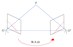
Figure 10: Epipolar geometry of the real and virtual cameras.

When the real and virtual cameras capture different views of a 3D scene in Figure 10, any point in the scene and the centers of the camera must lie on the same plane. This gives us the constraint:

$$\overrightarrow{O^{\prime}P}\cdot(\overrightarrow{O^{\prime}O}\times\overrightarrow{OP})=0$$ (24)

We can denote the coordinates of point $p$ under the real camera frame with origin $O$ to be $[x,y,z]^{T}$ and the coordinates under the right camera frame with origin $O^{\prime}$ to be $[x^{\prime},y^{\prime},z^{\prime}]^{T}$. Subsequently, we get the equation:

$$\begin{bmatrix}x^{\prime}\\ y^{\prime}\\ z^{\prime}\end{bmatrix}^{\mathsf{T}}\left(\mathbf{D}\mathbf{t}\times(\mathbf{D}\mathbf{R}\begin{bmatrix}x\\ y\\ z\end{bmatrix})\right)=0$$ (25)

where

$$\mathbf{D}=\begin{bmatrix}-1&0&0\\ 0&1&0\\ 0&0&1\end{bmatrix}$$ (26)

Accounting for the projection geometry and using $\mathbf{K}$ to denote the intrinsic matrix, the following restrictions can be derived:

$$\begin{bmatrix}x\\ y\\ z\end{bmatrix}=\mathbf{z}\mathbf{K}^{-1}\begin{bmatrix}u\\ v\\ 1\end{bmatrix},\begin{bmatrix}x^{\prime}\\ y^{\prime}\\ z^{\prime}\end{bmatrix}=\mathbf{z^{\prime}}\mathbf{K}^{-1}\begin{bmatrix}u^{\prime}\\ v^{\prime}\\ 1\end{bmatrix},$$ (27)

$$\begin{bmatrix}u^{\prime}\\ v^{\prime}\\ 1\end{bmatrix}\mathbf{K}^{-T}\mathbf{E}\mathbf{K}^{-1}\begin{bmatrix}u\\ v\\ 1\end{bmatrix}=0$$ (28)

After we have got the fundamental matrix $\mathbf{F}$, we can obtain the essential matrix by $\mathbf{E}=\mathbf{K}^{\mathsf{T}}\mathbf{F}\mathbf{K}$. Let $\mathbf{t^{\prime}}$ be written as:

$$\mathbf{t^{\prime}}=\mathbf{D}\mathbf{t}$$ (29)

Then the Essential matrix is as follows:

$$\mathbf{E}=[\mathbf{t^{\prime}}]_{\times}\mathbf{D}\mathbf{R}$$ (30)

where $[\mathbf{t^{\prime}}]_{\times}$ is a skew-symmetric matrix and can be written as:

$$[\mathbf{t^{\prime}}]_{\times}=\mathbf{U}diag(1,1,0)\mathbf{W}^{\mathsf{T}}\mathbf{U}^{\mathsf{T}},\mathbf{W}=\begin{bmatrix}0&-1&0\\ 1&0&0\\ 0&0&1\end{bmatrix}$$ (31)

or

$$[\mathbf{t^{\prime}}]_{\times}=-\mathbf{U}diag(1,1,0)\mathbf{W}\mathbf{U}^{\mathsf{T}},$$ (32)

$\mathbf{U}$ is an orthogonal matrix in Equations (31) and (32). And according to Equations (30), (31), and (32), there are two possibilities for the essential matrix:

$$\mathbf{E} =\mathbf{U}diag(1,1,0)\mathbf{W}^{\mathsf{T}}\mathbf{U}^{\mathsf{T}}\begin{bmatrix}-1&0&0\\ 0&1&0\\ 0&0&1\end{bmatrix}\mathbf{R}$$ (33)

$$=\mathbf{U}diag(1,1,0)\mathbf{V}^{\mathsf{T}}_{1}$$

and:

$$\mathbf{E} =\mathbf{U}diag(1,1,0)\left(-\mathbf{W}\mathbf{U}^{\mathsf{T}}\begin{bmatrix}-1&0&0\\ 0&1&0\\ 0&0&1\end{bmatrix}\mathbf{R}\right)$$ (34)

$$=\mathbf{U}diag(1,1,0)\mathbf{V}^{\mathsf{T}}_{2}$$

Note that the matrices $\mathbf{V}^{\mathsf{T}}_{1}$ and $\mathbf{V}^{\mathsf{T}}_{2}$ are orthogonal. If we observe Equations (33) and (34), it reminds us of singular value decomposition. After singular value decomposition, from Equation (33), we can obtain the rotation matrix by:

$$\mathbf{R}_{1}=\begin{bmatrix}-1&0&0\\ 0&1&0\\ 0&0&1\end{bmatrix}\mathbf{U}\mathbf{W}\mathbf{V}^{\mathsf{T}}$$ (35)

or:

$$\mathbf{R}_{2}=-\begin{bmatrix}-1&0&0\\ 0&1&0\\ 0&0&1\end{bmatrix}\mathbf{U}\mathbf{W}^{\mathsf{T}}\mathbf{V}^{\mathsf{T}}$$ (36)

And translation $[\mathbf{t^{\prime}}]_{\times}$ can be obtained by:

$$[\mathbf{t^{\prime}}]_{\times}=\mathbf{U}diag(1,1,0)\mathbf{W}^{\mathsf{T}}\mathbf{U}^{\mathsf{T}}=-\mathbf{U}diag(1,1,0)\mathbf{W}\mathbf{U}^{\mathsf{T}}$$ (37)

Because $\mathbf{E}$ and $-\mathbf{E}$ both satisfy Equation (28), $-[\mathbf{t^{\prime}}]_{\times}$ is also a solution. In addition, we can easily obtain $\mathbf{t}$ from $[\mathbf{t^{\prime}}]_{\times}$. Note that there exist four possible combinations of $\mathbf{R}$ and $\mathbf{t}$ that can yield a solution. However, the correct combination can be determined by verifying whether the reconstructed points are positioned behind the cameras after triangulation. This decomposition algorithm is modified according to our scenario from a previous study [22].

Longyun Liao is a Ph.D. Candidate in the Computing and Software Department of McMaster University, Hamilton, ON, Canada since 2021. She received her B.S. degree in Electrical Engineering from McGill University in 2019 and her MSc degree in Imperial College London in 2020. Her research interest lies at the intersection of machine learning and computer vision, with a focus on 3D human pose estimation.

Andrew Mitchell is a Computer Science Ph.D. Candidate in the Department of Computing and Software at McMaster University. He completed a Bachelor of Applied Science in Computer Science in 2021, and a Bachelor of Arts in Philosophy in 2017, both also at McMaster University. His primary areas of interest are human pose estimation, and the application of deep learning to solve real-world problems.

Rong Zheng is a Professor in the Department of Computing and Software, an associate member of the Department of Electrical and Computer Engineering, and a member of the School of Biomedical Engineering in McMaster University, Canada. She was on the faculty of the Department of Computer Science, University of Houston from 2004 to 2012. Rong Zheng was a visiting Associate Professor in the Hong Kong Polytechnic University from Aug. 2011 to Jan. 2012; and a visiting Research Scientist in Microsoft Research, Redmond between Feb. 2012 and May 2012. Her research interests include mobile computing, active machine learning and networked systems.

References

- [1] R. Rodrigues, J. P. Barreto, and U. Nunes, “Camera pose estimation using images of Planar Mirror Reflections,” Computer Vision – ECCV 2010, pp. 382–395, 2010.
- [2] K. Takahashi, S. Nobuhara, and T. Matsuyama, “A new mirror-based extrinsic camera calibration using an orthogonality constraint,” in Proceedings of the IEEE Computer Society Conference on Computer Vision and Pattern Recognition, 2012.
- [3] R. K. Kumar, A. Ilie, J. M. Frahm, and M. Pollefeys, “Simple calibration of non-overlapping cameras with a mirror,” in 26th IEEE Conference on Computer Vision and Pattern Recognition, CVPR, 2008.
- [4] G. Long, L. Kneip, X. Li, X. Zhang, and Q. Yu, “Simplified mirror-based camera pose computation via rotation averaging,” in Proceedings of the IEEE Computer Society Conference on Computer Vision and Pattern Recognition, 2015, vol. 07-12-June-2015.
- [5] A. Agrawal and S. Ramalingam, “Single image calibration of multi-axial imaging systems,” in Proceedings of the IEEE Computer Society Conference on Computer Vision and Pattern Recognition, 2013. doi: 10.1109/CVPR.2013.184.
- [6] S. A. Nene and S. K. Nayar, “Stereo with mirrors,” in Proceedings of the IEEE International Conference on Computer Vision, 1998. doi: 10.1109/iccv.1998.710852.
- [7] J. Gluckman and S. K. Nayar, “Catadioptric stereo using planar mirrors,” Int J Comput Vis, vol. 44, no. 1, 2001, doi: 10.1023/A:1011172403203.
- [8] T. Tahara, R. Kawahara, S. Nobuhara, and T. Matsuyama, “Interference-Free Epipole-Centered Structured Light Pattern for Mirror-Based Multi-view Active Stereo,” in Proceedings - 2015 International Conference on 3D Vision, 3DV 2015, 2015. doi: 10.1109/3DV.2015.25.
- [9] D. Lanman, D. Crispell, and G. Taubin, “Surround structured lighting: 3-D scanning with orthographic illumination,” Computer Vision and Image Understanding, vol. 113, no. 11, 2009, doi: 10.1016/j.cviu.2009.03.016.
- [10] X. Ying, K. Peng, Y. Hou, S. Guan, J. Kong, and H. Zha, “Self-calibration of catadioptric camera with two planar mirrors from silhouettes,” IEEE Trans Pattern Anal Mach Intell, vol. 35, no. 5, 2013, doi: 10.1109/TPAMI.2012.195.
- [11] J. Puwein, L. Ballan, R. Ziegler, and M. Pollefeys, “Joint Camera Pose Estimation and 3D human pose estimation in a multi-camera setup,” Computer Vision – ACCV 2014, pp. 473–487, 2015.
- [12] K. Takahashi, D. Mikami, M. Isogawa, and H. Kimata, “Human pose as calibration pattern: 3D human pose estimation with multiple unsynchronized and uncalibrated cameras,” in IEEE Computer Society Conference on Computer Vision and Pattern Recognition Workshops, 2018, vol. 2018-June. doi: 10.1109/CVPRW.2018.00230.
- [13] B. Huang, Y. Shu, T. Zhang, and Y. Wang, “Dynamic Multi-Person Mesh Recovery from Uncalibrated Multi-View Cameras,” in Proceedings - 2021 International Conference on 3D Vision, 3DV 2021, 2021. doi: 10.1109/3DV53792.2021.00080.
- [14] G. Ben-Artzi, Y. Kasten, S. Peleg, and M. Werman, “Camera Calibration from Dynamic Silhouettes Using Motion Barcodes,” in Proceedings of the IEEE Computer Society Conference on Computer Vision and Pattern Recognition, 2016, vol. 2016-December. doi: 10.1109/CVPR.2016.444.
- [15] S. N. Sinha and M. Pollefeys, “Camera network calibration and synchronization from silhouettes in archived video,” Int J Comput Vis, vol. 87, no. 3, 2010, doi: 10.1007/s11263-009-0269-2.
- [16] G. L. Mariottini, S. Scheggi, F. Morbidi, and D. Prattichizzo, “Planar mirrors for image-based robot localization and 3-D reconstruction,” Mechatronics, vol. 22, no. 4, 2012
- [17] R. I. Hartley, “In defence of the 8-point algorithm,” in IEEE International Conference on Computer Vision, 1995.
- [18] J. Wang et al., “Deep High-Resolution Representation Learning for Visual Recognition,” IEEE Trans Pattern Anal Mach Intell, vol. 43, no. 10, 2021.
- [19] M. Loper, N. Mahmood, J. Romero, G. Pons-Moll, and M. J. Black, “SMPL: A skinned multi-person linear model,” in ACM Transactions on Graphics, 2015, vol. 34, no. 6.
- [20] C. Ionescu, D. Papava, V. Olaru, and C. Sminchisescu, “Human3. 6M,” IEEE Transactions on Pattern Analysis and Machine Intelligence, 2014.
- [21] K. M. Robinette, H. Daanen, and E. Paquet, “The CAESAR project: A 3-D surface anthropometry survey,” in Proceedings - 2nd International Conference on 3-D Digital Imaging and Modeling, 3DIM 1999, 1999. doi: 10.1109/IM.1999.805368.
- [22] R. Y. Tsai and T. S. Huang, “Uniqueness and Estimation of Three-Dimensional Motion Parameters of Rigid Objects with Curved Surfaces,” IEEE Trans Pattern Anal Mach Intell, vol. PAMI-6, no. 1, 1984, doi: 10.1109/TPAMI.1984.4767471.
- [23] Q. Fang, Q. Shuai, J. Dong, H. Bao, and X. Zhou, “Reconstructing 3D human pose by watching humans in the mirror,” in Proceedings of the IEEE Computer Society Conference on Computer Vision and Pattern Recognition, 2021. doi: 10.1109/CVPR46437.2021.01262.
- [24] G. Bradski, “The OpenCV Library,” Dr. Dobb’s Journal of Software Tools, 2000.
- [25] Z. Cao, G. Hidalgo, T. Simon, S.-E. Wei, and Y. Sheikh, “OpenPose: Realtime multi-person 2D pose estimation using part affinity fields,” IEEE Transactions on Pattern Analysis and Machine Intelligence, vol. 43, no. 1, pp. 172–186, 2021.
- [26] P. Sturm and T. Bonfort, “How to compute the pose of an object without a direct view?,” Computer Vision – ACCV 2006, pp. 21–31, 2006.
- [27] G. Varol et al., “Learning from synthetic humans,” in Proceedings - 30th IEEE Conference on Computer Vision and Pattern Recognition, CVPR 2017, 2017. doi: 10.1109/CVPR.2017.492.
- [28] K. H. Jang, Y. M. Cha, and S. K. Jung, “3D reconstruction using moving planar mirror,” in IASTED International Conference on Computer Graphics and Imaging, 2003.
- [29] M. Kanbara, N. Ukita, M. Kidode, and N. Yokoya, “3D scene reconstruction from reflection images in a spherical mirror,” in Proceedings - International Conference on Pattern Recognition, 2006. doi: 10.1109/ICPR.2006.32.
- [30] H. Zhong, W. F. Sze, and Y. S. Hung, “Reconstruction from plane mirror reflection,” in Proceedings - International Conference on Pattern Recognition, 2006. doi: 10.1109/ICPR.2006.981.
- [31] B. Hu, “It’s all done with mirrors: calibration- and- correspondence- free 3D reconstruction,” in Proceedings of the 2009 Canadian Conference on Computer and Robot Vision, CRV 2009, 2009. doi: 10.1109/CRV.2009.29.
- [32] Y. Zhang, C. Wang, X. Wang, W. Liu, and W. Zeng, “VoxelTrack: Multi-Person 3D Human Pose Estimation and Tracking in the Wild,” IEEE Trans Pattern Anal Mach Intell, vol. 45, no. 2, 2023, doi: 10.1109/TPAMI.2022.3163709.
- [33] C. Lassner, J. Romero, M. Kiefel, F. Bogo, M. J. Black, and P. V. Gehler, “Unite the people: Closing the loop between 3D and 2D human representations,” in Proceedings - 30th IEEE Conference on Computer Vision and Pattern Recognition, CVPR 2017, 2017. doi: 10.1109/CVPR.2017.500.
- [34] M. Andriluka, L. Pishchulin, P. Gehler, and B. Schiele, “2D human pose estimation: New benchmark and state of the art analysis,” in Proceedings of the IEEE Computer Society Conference on Computer Vision and Pattern Recognition, 2014. doi: 10.1109/CVPR.2014.471.
- [35] T.-Y. Lin et al., “Microsoft COCO: Common Objects in Context,” Proceedings of the IEEE Computer Society Conference on Computer Vision and Pattern Recognition, 2015.
- [36] M. Fieraru, M. Zanfir, S. C. Pirlea, V. Olaru, and C. Sminchisescu, “AIFit: Automatic 3D Human-Interpretable Feedback Models for Fitness Training,” in Proceedings of the IEEE Computer Society Conference on Computer Vision and Pattern Recognition, 2021. doi: 10.1109/CVPR46437.2021.00979.
- [37] C. Sminchisescu, “3D Human motion analysis in monocular video techniques and challenges,” in Proceedings - IEEE International Conference on Video and Signal Based Surveillance 2006, AVSS 2006, 2006. doi: 10.1109/AVSS.2006.3.
- [38] Y. Goutsu and T. Inamura, “Linguistic Descriptions of Human Motion with Generative Adversarial Seq2Seq Learning,” in Proceedings - IEEE International Conference on Robotics and Automation, 2021. doi: 10.1109/ICRA48506.2021.9561519.
- [39] W. Takano and Y. Nakamura, “Statistical mutual conversion between whole body motion primitives and linguistic sentences for human motions,” International Journal of Robotics Research, vol. 34, no. 10, 2015, doi: 10.1177/0278364915587923.
- [40] S. J. D. Prince, Computer Vision: Models, Learning, and Inference. New York: Cambridge University Press, 2014.
- [41] S. Beckouche, S. Leprince, N. Sabater, and F. Ayoub, “Robust outliers detection in image point matching,” in Proceedings of the IEEE International Conference on Computer Vision, 2011. doi: 10.1109/ICCVW.2011.6130241.