Estimation of Semiparametric Multi–Index Models
Using Deep Neural Networks

Chaohua Dong^∗, Jiti Gao^†, Bin Peng^† and Yayi Yan^♯

^∗Zhongnan University of Economics and Law

^†Monash University

^♯Shanghai University of Finance and Economics

In this paper, we consider estimation and inference for both the multi-index parameters and the link function involved in a class of semiparametric multi–index models via deep neural networks (DNNs). We contribute to the design of DNN by i) providing more transparency for practical implementation, ii) defining different types of sparsity, iii) showing the differentiability, iv) pointing out the set of effective parameters, and v) offering a new variant of rectified linear activation function (ReLU), etc. Asymptotic properties for the joint estimates of both the index parameters and the link functions are established, and a feasible procedure for the purpose of inference is also proposed. We conduct extensive numerical studies to examine the finite-sample performance of the estimation methods, and we also evaluate the empirical relevance and applicability of the proposed models and estimation methods to real data.

Keywords: Asymptotic Theory; Multi-Index Model; ReLU; Semiparametric Regression

1 Introduction

In recent decades, there has been a notable emphasis on deep neural networks (DNNs). Initially applied in machine learning, DNNs have since expanded into various fields, such as economics, finance, social sciences, among others. Related to the applications of DNN, LeCun et al. (2015) offer a comprehensive overview of practical topics, while Athey (2019) discusses its capacity in social science. Additionally, Bartlett et al. (2021) and Fan et al. (2021) provide summaries of recent methodological advancements.

As the most important part of DNN, a variety of activation functions have been proposed and investigated theoretically and numerically (Dubey et al., 2022). The rectified linear activation function (ReLU) sees its popularity due to its simplicity and partial linearity:

$$\sigma(x)=x\vee 0\quad\text{with}\quad x\in\mathbb{R}.$$

ReLU is a piecewise linear function that will output the input directly if it is positive, otherwise, it will output zero. Compared to Sigmoid functions, ReLU has a low computational cost, which makes it efficient for large-scale neural networks practically. Schmidt-Hieber (2020), Farrell et al. (2021) and Fan and Gu (2022) for example establish some fundamental results with respect to using ReLU.

However, there are still properties related to ReLU that remain unknown. To be more specific, we now define a simple DNN using ReLU for activation function, and then briefly review the relevant literature.

Definition 1.1 (Simple DNN).

For $\forall\mathbf{x},\mathbf{v}\in\mathbb{R}^{n}$, define the shifted activation function $\boldsymbol{\sigma}_{\mathbf{v}}:\mathbb{R}^{n}\to\mathbb{R}^{n}$ as

$$\boldsymbol{\sigma}_{\mathbf{v}}(\mathbf{x})=(\sigma(x_{1}-v_{1}),\ldots,\sigma(x_{n}-v_{n}))^{\top},$$

where $x_{j}$ and $v_{j}$ stand for the $j^{th}$ elements of $\mathbf{x}$ and $\mathbf{v}$ respectively. A simple DNN with $m$ hidden layers that realizes the mapping $\mathbb{U}\,(\subseteq\mathbb{R}^{c_{1}})\mapsto\mathbb{R}$ is defined as follows:

Mathematically, it is written as

$$\operatorname*{\mathcal{N}}(\mathbf{x}\,|\,\mathbf{W}_{m}) := \mathbf{w}_{m}\,\boldsymbol{\sigma}_{\mathbf{v}_{m}}\,\cdots\,\mathbf{w}_{1}\,\boldsymbol{\sigma}_{\mathbf{v}_{1}}(\mathbf{x}),$$

where $\mathbf{W}_{m}:=\{\mathbf{v}_{1},\ldots,\mathbf{v}_{m};\mathbf{w}_{1},\ldots,\mathbf{w}_{m}\}$, and the weighting matrices and shit vectors have the following dimensions:

$$\mathbf{w}_{j}\text{ is }\left\{\begin{array}[]{ll}c_{1}\times c_{1}&\text{for }j=1,\\ c_{j}\times c_{j-1}&\text{for }2\leq j\leq m-1,\\ 1\times c_{m-1}&\text{for }j=m,\end{array}\right.\quad\text{and}\quad\mathbf{v}_{j}\text{ is }\left\{\begin{array}[]{ll}c_{1}\times 1&\text{for }j=1,\\ c_{j-1}\times 1&\text{for }j\geq 2.\end{array}\right.$$

The current literature agrees that ReLU is designed to provide sparsity, which leads to computational efficiency (e.g., Glorot et al., 2011; Schmidt-Hieber, 2020). However, there has been few efforts to explain how sparsity should be defined and why it occurs. To the best of our understanding, there are at least two types of sparsity involved: (1) non-active neurons and (2) parameters that are not effective. Additionally, the literature implicitly agrees that $\mathbf{W}_{m}$ can be estimated through a minimization process (e.g., eq. (2.4) of Farrell et al., 2021). It is noteworthy that ReLU is piecewise linear, and it is not yet clear how to handle the accumulated (non)differentiability through layers in both theory and practice. While the concern raised here actually exits in some well known software packages, to the best of our knowledge, no satisfactory treatment has been offered. For example, the well known neuralnet in R does not even support the use of ReLU (Günther and Fritsch, 2010). PyTorch does have ReLU and some of its variations included as the activation functions, but the explanation about the optimization process is very vague (https://pytorch.org/docs/stable/optim.html). Keras includes Adam algorithm and its variations (https://keras.io/api/optimizers/adam/), but Adam requires “a stochastic scalar function that is differentiable w.r.t. parameters…” (Kingma and Ba, 2015), which does not apply to ReLU directly in an obvious manner. A comprehensive survey on the alternatives of ReLU is provided by Dubey et al. (2022), who comment on the pros and cons of different activation functions from the perspective of implementation. We aim to settle some of these concerns in the paper.

Moving on to our discussion about modelling data, when it comes to practical analysis using DNN based models and methods, the existing literature of model building primarily focuses on fully nonparametric models, with only a few mentions of semiparametric settings (e.g., Kohler and Krzyźak (2017); Bauer and Kohler (2019), and references therein). It is not clear how to estimate and recover the index parameters involved in such semiparametric hierarchical interaction models, and there is a lack of investigations in this area of research. This issue is also related to the (non)differentiability of ReLU. As far as we know, these questions have not been thoroughly investigated.

Meanwhile, the current literature heavily focuses on independent and identically distributed (i.i.d.) data, while largely neglecting the implications of asymptotic properties when dealing with dependent data. This is especially significant for applications in the fields of finance and economics, such as those studied by Kaastra and Boyd (1996) and Gu et al. (2020), where accounting for dependence can pose challenges in constructing inference. The literature on this topic dates at least back to Newey and West (1987), with a comprehensive review provided by Shao (2015). In the paper, we aim to address this gap by training DNN with time series data, establishing asymptotic properties, and providing valid inference.

In what follows, in order to address the aforementioned concerns collectively, we consider a semiparametric hierarchical interaction model of the form:

$$y_{t}=f_{\star}(\mathbf{z}_{1t}^{\top}\,\boldsymbol{\theta}_{\star 1},\ldots,\mathbf{z}_{rt}^{\top}\,\boldsymbol{\theta}_{\star r})+\varepsilon_{t},\ t=1,2,\cdots,T,$$ (1.2)

where $f_{\star}(\cdot)$ is an unknown link function of $r$–dimensional components, $(\theta_{\star 1},\cdots,\theta_{\star r})$ is a vector of unknown index parameters, each $\mathbf{z}_{jt}$ is a $d_{j}\times 1$ observed time series with $d_{j}\geq 2$, and $\varepsilon_{t}$ is an idiosyncratic error term.

Throughout the rest of this paper, we suppose that $d_{j}$’s and $r$ are finite, although $d_{j}$’s may be very large and much larger than $r$. One of the main features of our models (1.2) and (1.3) is that the multi–index setting may significantly reduce the dimensionality from $d=\sum_{j=1}^{r}d_{j}$ to $r$. We also assign the script $\star$ to the true parameters and the true function. For the purpose of identification, let $\|\boldsymbol{\theta}_{\star j}\|=1$ for all $j$’s, and let the first elements of $\boldsymbol{\theta}_{\star j}$’s be positive.

While model (1.2) has been proposed for the estimation of the link function, $f_{\ast}(\cdot)$, in the relevant DNN literature (see, for example, Kohler and Krzyźak (2017); Bauer and Kohler (2019)), to the best of our knowledge, there have been no attempts to estimate $(\theta_{\star 1},\cdots,\theta_{\star r})$ as a vector of the index parameters of interest. The main goals are to estimate and recover both $f_{\star}(\cdot)$ and $\boldsymbol{\theta}_{\star j}$’s jointly using a ReLU based DNN approach.

When no misunderstanding arises, we write (1.2) as

$$y_{t}=f_{\star}(\mathbf{z}_{t}\,\boldsymbol{\theta}_{\star})+\varepsilon_{t}$$ (1.3)

for notational simplicity, with $\mathbf{z}_{t}=\operatorname*{\textrm{diag}}\{\mathbf{z}_{1t}^{\top},\ldots,\mathbf{z}_{rt}^{\top}\}$ returning a block wise diagonal matrix, and $\boldsymbol{\theta}_{\star}=(\boldsymbol{\theta}_{\star 1}^{\top},\ldots,\boldsymbol{\theta}_{\star r}^{\top})^{\top}$ being a $d\times 1$ vector with $d=\sum_{j=1}^{r}d_{j}$.

Up to this point, it is worth mentioning that there is a vast literature about non– and semi–parametric index settings via unknown link functions, e.g., Xia et al. (1999). Hristache et al. (2001), Gao (2007), Horowitz and Mammen (2007), Xia (2008), Ma and Song (2015), Dong et al. (2016), Ma and He (2016), and Zhou et al. (2023). Our investigation of model (1.2) adds to the relevant literature by introducing a unified DNN based approach to the estimation of both the index parameters and the link function. The main advantage of the proposed DNN based estimation method is that we are probably among the first in being able to estimate and recover both the index parameters and the link function jointly and consistently in comparison with the existing DNN based estimation methods.

Moreover, the proposed DNN based estimation method offers a unified way to deal with the case where the dimensionality of $f_{\star}(\cdot)$, $r$, can be large (although being fixed). By contrast, the existing nonparametric methods suffer from the so–called “curse of dimensionality” issue when $r\geq 4$, for example. As a consequence of our discussion, we are also able to offer insights on how to generalize the approach to a broader class of models, including factor augmented models studied by Bernanke et al. (2005) and Fu et al. (2023), which are of great interest. To see this, we will also delve into an example in the following instance.

Example 1.

Consider (1.2) and let $r=2$:

$$y_{t}=f_{\star}(\mathbf{z}_{1t}^{\top}\,\boldsymbol{\theta}_{\star 1},\mathbf{z}_{2t}^{\top}\,\boldsymbol{\theta}_{\star 2})+\varepsilon_{t}.$$

In this example, we suppose that $\mathbf{z}_{1t}$ and $\mathbf{z}_{2t}$ are observable and unobservable vectors respectively, and $\mathbf{z}_{2t}$ is from the following low rank representation:

$$\mathbf{X}_{t}=\boldsymbol{\Lambda}\,\mathbf{z}_{2t}+\mathbf{V}_{t}.$$

Here, $\mathbf{X}_{t}$ is a $n\times 1$ observable vector, and $n$ may diverge. Consequently, $\boldsymbol{\Lambda}$ and $\mathbf{V}_{t}$ are $n\times d_{2}$ and $n\times 1$ respectively. We let $d_{2}$ be known for simplicity. There is a rich literature discussing the estimation of $d_{2}$ when it is unknown (e.g., Bai and Ng, 2002; Lam and Yao, 2012; Ahn and Horenstein, 2013). This example extends the typical factor augmented model to a nonparametric framework, following the approach of Horowitz and Mammen (2007), Xia (2008), and Fan and Gu (2022) in terms of dimension reduction.

In summary, our study makes the following main contributions:

1. We enhance the design of DNN by i) providing more transparency for practical implementation, ii) defining different types of sparsity, iii) showing the differentiability, iv) pointing out the set of effective parameters, and v) offering a new variant of ReLU, etc.

2. We investigate a class of semiparametric hierarchical interaction models using a ReLu based DNN approach. A set of asymptotic properties for the joint estimation of both the index parameters and the link function are established, and can be applicable to a wide class of non– and semi–parametric settings.

3. We allow our models and methods to be applicable to dependent time series data and then establish a valid implementational procedure for the purpose of inference.

4. We conduct extensive numerical results to validate the theoretical findings before we also demonstrate the empirical relevance and applicability of the proposed model and estimation method to real data.

The remainder of this paper is structured as follows. Section 2 presents the design of DNN, and establishes some basic results which can be applied to a wide class of nonparametric models. Section 3 considers the estimation of model (1.2), and derives the asymptotics accordingly. In Section 4, we point out a few possible extensions. Section 5 provides extensive numerical studies to examine the theoretical findings. We conclude in Section 6 with a few remarks. Due to space limit, we provide extra plots, and give the proofs in Appendix B1.1 and Appendix B2 respectively in the online supplementary file.

Before proceeding further, we introduce a few notations which will be repeatedly used throughout the paper.

Symbols & basic operations — For $\forall w\in\mathbb{R}$, we let $\lfloor w\rfloor$ and $\lceil w\rceil$ be the largest and smallest integers satisfying $\lfloor w\rfloor\leq w$ and $\lceil w\rceil\geq w$ respectively. For $\forall n\in\mathbb{N}$, we let $\mathbf{I}_{n}$, $\mathbf{1}_{n}$, and $[n]$ be a $n\times n$ identify matrix, a $n\times 1$ vector of ones, and a set $\{1,2,\ldots,n\}$ respectively. For $\boldsymbol{\alpha}\in\mathbb{N}_{0}^{r}$ with $\mathbb{N}_{0}=0\cup\mathbb{N}$ and $\mathbf{x}\in\mathbb{R}^{r}$, we let

$$\boldsymbol{\alpha}!=\prod_{i=1}^{r}\alpha_{i}!,\quad\mathbf{x}^{\boldsymbol{\alpha}}=\prod_{i=1}^{r}x_{i}^{\alpha_{i}},\quad\|\mathbf{x}\|_{1}=\sum_{i=1}^{r}|x_{i}|,$$

$$\boldsymbol{\ell}_{\mathbf{x}\,|\,{\boldsymbol{\alpha}}}=(x_{1}^{\alpha_{1}},\ldots,x_{r}^{\alpha_{r}},\mathbf{1}_{q}^{\top})^{\top}\quad\text{with}\quad q=\left\{\begin{array}[]{ll}2^{\lceil\log_{2}r\rceil}-r&\text{for }r\geq 2\\ 1&\text{for }r=1\end{array}\right..$$

For a matrix $\mathbf{A}$, we let $\|\mathbf{A}\|$ and $\|\mathbf{A}\|_{2}$ define its Frobenius norm and Spectral norm respectively. Throughout, we write

$$\mathbf{z}_{t}^{\top}\mathbf{1}_{r}:=\widetilde{\mathbf{z}}_{t}\quad\text{and}\quad I_{a,t}=I(\mathbf{z}_{t}\,\boldsymbol{\theta}_{\star}\in[-a,a]^{r})\quad\text{for}\quad t\in[T].$$

Function operations & monomials — Let $f(\mathbf{x})$ be a sufficiently smooth function defined on $\mathbb{U}\subseteq\mathbb{R}^{r}$, and define

$$\|f\|_{\infty}^{\mathbb{U}}=\sup_{\mathbf{x}\in\mathbb{U}}|f(\mathbf{x})|,\quad f^{(\boldsymbol{\alpha})}(\mathbf{x})=\frac{\partial^{\|\boldsymbol{\alpha}\|_{1}}f(\mathbf{x})}{\partial x_{r}^{\alpha_{r}}\cdots\partial x_{1}^{\alpha_{1}}},$$

$$\mathbf{f}^{(1)}(\mathbf{x})=\operatorname*{\textrm{diag}}\Big{\{}\frac{\partial f(\mathbf{x})}{\partial x_{1}}\mathbf{I}_{d_{1}},\ldots,\frac{\partial f(\mathbf{x})}{\partial x_{r}}\mathbf{I}_{d_{r}}\Big{\}}.$$

We define a space of monomials:

$$\mathscr{P}_{n}=\left\{\text{Linear span of $\mathbf{x}^{\boldsymbol{\alpha}}$ with $0\leq|\boldsymbol{\alpha}|\leq n$}\right\},$$

of which the dimension is $\text{dim}\mathscr{P}_{n}=\binom{r+n}{r}:=r_{n}$ by direct calculation. Denote the basis of $\mathscr{P}_{n}$ by $\{\psi_{1}(\mathbf{x}),\ldots,\psi_{r_{n}}(\mathbf{x})\}$, and let

$$\boldsymbol{\psi}_{r_{n}}(\mathbf{x})=(\psi_{1}(\mathbf{x}),\ldots,\psi_{r_{n}}(\mathbf{x}))^{\top}.$$

For $\forall\mathbf{x}_{0}\in\mathbb{U}$, define the re-centred basis by $\{\psi_{1}(\mathbf{x}\,|\,\mathbf{x}_{0}),\ldots,\psi_{r_{n}}(\mathbf{x}\,|\,\mathbf{x}_{0})\}$, and let

$$\boldsymbol{\psi}_{r_{n}}(\mathbf{x}\,|\,\mathbf{x}_{0})=(\psi_{1}(\mathbf{x}\,|\,\mathbf{x}_{0}),\ldots,\psi_{r_{n}}(\mathbf{x}\,|\,\mathbf{x}_{0}))^{\top}.$$

Having these notation and symbols in hand, we are now ready to start our investigation.

2 DNN via ReLU

In this section, we present the design of DNN, and establish some basic results which can be applied to a wide class of nonparametric models. Specifically, Section 2.1 provides some basic definitions, while Section 2.2 presents the detailed design.

2.1 Basic Definitions

Recall that we have defined a simple DNN (i.e., $\operatorname*{\mathcal{N}}(\cdot\,|\,\mathbf{W}_{m})$) in Definition 1.1. Building on it, we further define a pair-wise hierarchical DNN (referred to as HDNN hereafter), which plays an important role in what follows.

Definition 2.1 (HDNN).

Define a mapping $\boldsymbol{\ell}_{x,y}:(x,y)\mapsto\mathbb{U}$, where $x$ and $y$ are scalars. For $\forall\mathbf{u}=(u_{1},\ldots,u_{2^{q}})^{\top}$ with $q\in\mathbb{N}$, the HDNN (written as $\operatorname*{\mathcal{N}}_{\boldsymbol{\ell}}(\mathbf{u}\,|\,\mathbf{W}_{m})$) is implemented as follows:

1. Step 1 – Divide $\mathbf{u}$ into pairs, and calculate $\operatorname*{\mathcal{N}}(\boldsymbol{\ell}_{u_{1},u_{2}}\,|\,\mathbf{W}_{m}),\ldots,\operatorname*{\mathcal{N}}(\boldsymbol{\ell}_{u_{2^{q}-1},u_{2^{q}}}\,|\,\mathbf{W}_{m})$;

2. Step $n\ (2\leq n\leq q)$ – Apply $\operatorname*{\mathcal{N}}(\boldsymbol{\ell}_{x,y}\,|\,\mathbf{W}_{m})$ to each pair of the outcomes from Step $n-1$.

To better see Definition 2.1, we plot Figure 1 for the purpose of visualization.

Figure 1: HDNN of Definition 2.1

In Figure 1, it is obvious that after $q$ steps, there is only one scalar left, which is the output of HDNN. Thus, the total number of hidden layers is $mq$. Although $\operatorname*{\mathcal{N}}_{\boldsymbol{\ell}}(\mathbf{u}\,|\,\mathbf{W}_{m})$ may appear complex, its parameters are entirely determined by $\mathbf{W}_{m}$ and $\boldsymbol{\ell}_{x,y}$. Consequently, the number of effective parameters is significantly less than it appears. Finally, the ordering of the elements in $\mathbf{u}$ does not matter.

We next regulate the unknown function that is to be estimated.

Definition 2.2 (Smoothness).

Let $p=\vartheta+s$ for some $\vartheta\in\mathbb{N}$ and $0<s\leq 1$, and $\mathbb{U}\subseteq\mathbb{R}^{r}$. A function $f\,:\,\mathbb{U}\mapsto\mathbb{R}$ is called $(p,\mathscr{C})$-smooth, if for $\forall\boldsymbol{\alpha}\in\mathbb{N}_{0}^{r}$ with $\|\boldsymbol{\alpha}\|_{1}=\vartheta$ the partial derivative $f^{(\boldsymbol{\alpha})}(\mathbf{x})$ exists and satisfies that

$$\|f^{(\boldsymbol{\alpha})}(\mathbf{x})-f^{(\boldsymbol{\alpha})}(\mathbf{z})\|_{\infty}^{\mathbb{U}}\leq\mathscr{C}\|\mathbf{x}-\mathbf{z}\|^{s},$$

where $\mathscr{C}$ is a constant.

Definition 2.2 is adopted from Bauer and Kohler (2019), and has different names in the literature (e.g., Hölder smoothness in Schmidt-Hieber, 2020; the Hilbert function space in Dong and Linton, 2018). That said, the family of functions covered by Definition 2.2 is less restrictive than the existing literature.

2.2 The Design

We present the design of neural network in this subsection, and establish some fundamental results regarding function approximation. First, we present the following lemma building on Definition 1.1.

Lemma 2.1.

For $\forall(x,y)\in[0,1]^{2}$, construct a DNN with $m+3$ hidden layers:

$$\operatorname*{\mathcal{N}}(\boldsymbol{\ell}^{m}_{x,y}\,|\,\mathbf{W}^{\star}_{m+3})\quad\text{with}\quad\mathbf{W}^{\star}_{m+3}=\{\mathbf{v}_{1}^{\star},\ldots,\mathbf{v}_{m+3}^{\star};\mathbf{w}_{1}^{\star},\ldots,\mathbf{w}_{m+3}^{\star}\},$$

where

$$\boldsymbol{\ell}_{x,y}^{m}=\frac{1}{2}\left(\frac{x-y+1}{2},\ x-y+1,\ x+y+2^{-m},\ \frac{x+y}{2},\ x+y,\ \frac{1}{2}\right)^{\top},$$

$$\mathbf{v}_{k}^{\star}=\left\{\begin{array}[]{ll}\mathbf{1}_{2}\otimes(0,2^{1-2k},0)^{\top}&\text{for }k\in[m+1]\\ -1&\text{for }k\in\{m+2,m+3\}\end{array}\right.,$$

$$\mathbf{w}_{k}^{\star}=\left\{\begin{array}[]{ll}\mathbf{I}_{2}\otimes\widetilde{\mathbf{w}}&\text{for }k\in[m]\\ (-1,1,-1,1-1,1)&\text{for }k=m+1\\ -1&\text{for }k=m+2\\ 1&\text{for }k=m+3\end{array}\right.,$$

$$\widetilde{\mathbf{w}}=\begin{pmatrix}\frac{1}{2}&-\frac{1}{2}&0\\ 1&-1&0\\ 1&-1&1\end{pmatrix}.$$

Here, $\operatorname*{\mathcal{N}}(\boldsymbol{\ell}^{m}_{x,y}\,|\,\mathbf{W}^{\star}_{m+3})$ is piecewise linear in $x$ and $y$, and $\frac{\partial}{\partial x}[\operatorname*{\mathcal{N}}(\boldsymbol{\ell}^{m}_{x,y}\,|\,\mathbf{W}^{\star}_{m+3})]$ is defined accordingly.

Let $\mathbb{C}_{m}=[0,1-2^{-m}]\times[0,1]$. The following results hold:

1. $0\leq\operatorname*{\mathcal{N}}(\boldsymbol{\ell}^{m}_{x,y}\,|\,\mathbf{W}^{\star}_{m+3})\leq 1$ on $[0,1]^{2}$, and $\operatorname*{\mathcal{N}}(\boldsymbol{\ell}^{m}_{x,y}\,|\,\mathbf{W}^{\star}_{m+3})=1$ at $(x,y)=(1,1)$,

2. $0\leq\operatorname*{\mathcal{N}}(\boldsymbol{\ell}^{m}_{x,y}\,|\,\mathbf{W}^{\star}_{m+3})-xy\leq 2^{-m}$ on $\mathbb{C}_{m}$,

3. $\left\|\frac{\partial}{\partial x}[\operatorname*{\mathcal{N}}(\boldsymbol{\ell}^{m}_{x,y}\,|\,\mathbf{W}^{\star}_{m+3})]-y\right\|_{\infty}^{\mathbb{C}_{m}}\leq 2^{-m-1}$.

In Lemma 2.1, $x$ and $y$ are symmetric in the sense that one can interchange $x$ and $y$ without violating the above results. In addition, Lemma 2.1 actually offers a generic result. For example, one can replace $y$ with a generic function, say $f(y)$, and the result still holds with obvious modification. Thus, $\operatorname*{\mathcal{N}}(\boldsymbol{\ell}^{m}_{x,y}\,|\,\mathbf{W}^{\star}_{m+3})$ offers a way to approximate different monomials practically, of which the space is the key to carry on nonparametric regression. To see this numerically, we plot Figure 2 in Section 5.1. Finally, it is worth mentioning that provided $\mathbb{C}_{m}$, $\operatorname*{\mathcal{N}}(\boldsymbol{\ell}^{m}_{x,y}\,|\,\mathbf{W}^{\star}_{m+3})$ always approximates $xy$ from positive side.

Based on Lemma 2.1, we are then able to further estimate different monomials. Specifically, we provide the following lemma.

Lemma 2.2.

Using $\operatorname*{\mathcal{N}}(\boldsymbol{\ell}^{m}_{x,y}\,|\,\mathbf{W}^{\star}_{m+3})$ of Lemma 2.1, define $\mathcal{N}_{\boldsymbol{\ell}^{m}}(\boldsymbol{\ell}_{\mathbf{x}\,|\,{\boldsymbol{\alpha}}}\,|\,\mathbf{W}^{\star}_{m+3})$ according to Definition 2.1, where $r\geq 2$, $\mathbf{x}\in[0,h]^{r}$, $h\leq 1-\lceil\log_{2}r\rceil\cdot 2^{-m}$, and $\boldsymbol{\alpha}\in\mathbb{N}_{0}^{r}$. Then the following results hold:

1. $0\leq\mathcal{N}_{\boldsymbol{\ell}^{m}}(\boldsymbol{\ell}_{\mathbf{x}\,|\,{\boldsymbol{\alpha}}}\,|\,\mathbf{W}^{\star}_{m+3})\leq 1$ uniformly on $\mathbf{x}\in[0,h]^{r}$,

2. $0\leq\mathcal{N}_{\boldsymbol{\ell}^{m}}(\boldsymbol{\ell}_{\mathbf{x}\,|\,{\boldsymbol{\alpha}}}\,|\,\mathbf{W}^{\star}_{m+3})-\mathbf{x}^{\boldsymbol{\alpha}}\leq 3^{\lceil\log_{2}r\rceil-1}2^{-m}$ uniformly on $\mathbf{x}\in[0,h]^{r}$,

3. $\|\frac{\partial}{\partial x_{i}}[\mathcal{N}_{\boldsymbol{\ell}^{m}}(\boldsymbol{\ell}_{\mathbf{x}\,|\,{\boldsymbol{\alpha}}}\,|\,\mathbf{W}^{\star}_{m+3})-\mathbf{x}^{\boldsymbol{\alpha}}]\|_{\infty}^{[0,h]^{r}}\leq 3^{\lceil\log_{2}r\rceil-1}\cdot\|\boldsymbol{\alpha}\|_{1}\cdot 2^{-m}$ for $\forall i\in[r]$.

Lemma 2.2 offers a specific range (i.e., $[0,h]^{r}$) in which DNN can approximate monomials reasonably well. It is interesting to note that the range includes non-negative quantities only, and $\mathcal{N}_{\boldsymbol{\ell}^{m}}(\boldsymbol{\ell}_{\mathbf{x}\,|\,{\boldsymbol{\alpha}}}\,|\,\mathbf{W}^{\star}_{m+3})$ converges to $\mathbf{x}^{\boldsymbol{\alpha}}$ from the positive side, which are consistent with Lemma 2.1. The construction of $\mathcal{N}_{\boldsymbol{\ell}^{m}}(\boldsymbol{\ell}_{\mathbf{x}\,|\,{\boldsymbol{\alpha}}}\,|\,\mathbf{W}^{\star}_{m+3})$ and Lemma 2.2.3 together offer a theoretical justification for Adam and Keras algorithms in which differentiability is required. In Section 5.1, we plot Figure 3 and Figure 4 for the purpose of demonstration.

We are now ready to consider the estimation of $f_{\star}(\mathbf{x})$. To proceed, we impose the following assumption to facilitate the development.

Assumption 1.

Let $f_{\star}(\mathbf{x})$ of (1.2) be $(p,\mathscr{C})$-smooth on $[-a,a]^{r}$, where $a\geq 0$ and $r\geq 1$ are fixed.

As explained under Definition 2.2, Assumption 1 is commonly adopted in the literature. To proceed, we recall the notation and symbols defined at the end of Section 1, and present the following lemma that approximates $f_{\star}(\mathbf{x})$.

Lemma 2.3.

Under Assumption 1, for $\forall\mathbf{x}_{0}\in[-a,a)^{r}$, there exits $\boldsymbol{\beta}_{\star}$ such that

$$\|f_{\star}(\mathbf{x})-\mathbf{N}(\mathbf{x}\,|\,\mathbf{x}_{0})^{\top}\boldsymbol{\beta}_{\star}\|_{\infty}^{C_{\mathbf{x}_{0},h}}=O(h^{p}+2^{-m}),$$

where $C_{\mathbf{x}_{0},h}=\{\mathbf{x}\,|\,\mathbf{x}-\mathbf{x}_{0}\in[0,h]^{r}\}$ with $h\to 0$, $\boldsymbol{\alpha}_{j}$’s are the power vectors of $\mathscr{P}_{r_{\vartheta}}$, and

$$\mathbf{N}(\mathbf{x}\,|\,\mathbf{x}_{0}) = \begin{pmatrix}\mathcal{N}_{\boldsymbol{\ell}^{m}}(\boldsymbol{\ell}_{\mathbf{x}-\mathbf{x}_{0}\,|\,\boldsymbol{\alpha}_{1}}\,|\,\mathbf{W}^{\star}_{m+3})\\ \vdots\\ \mathcal{N}_{\boldsymbol{\ell}^{m}}(\boldsymbol{\ell}_{\mathbf{x}-\mathbf{x}_{0}\,|\,\boldsymbol{\alpha}_{r_{\vartheta}}}\,|\,\mathbf{W}^{\star}_{m+3})\end{pmatrix}.$$

It should be understood that in Lemma 2.3, $\boldsymbol{\beta}_{\star}$ varies with respect to $\mathbf{x}_{0}$. Although $h\to 0$ is not required in Lemma 2.2, it is essential to include the condition here from the perspective of function approximation. Building on Lemma 2.3, for $\forall M\in\mathbb{N}$, we can subdivide $[-a,a]^{r}$ into $M^{r}$ cubes of side length $h=\frac{2a}{M}$. For comprehensibility, we label these cubes by $C_{\mathbf{x}_{\mathbf{i}}}$ with $\mathbf{i}\in[M]^{r}$, where $\mathbf{x}_{\mathbf{i}}$ represents the point at the bottom left corner of each cube. Mathematically, $C_{\mathbf{x}_{\mathbf{i}}}$ is expressed as

$$C_{\mathbf{x}_{\mathbf{i}}}=\{\mathbf{x}\,|\,\mathbf{x}-\mathbf{x}_{\mathbf{i}}\in[0,h]^{r}\}.$$ (2.3)

Using the partition, we further present the first theorem of this paper.

Theorem 2.1.

Let Assumption 1 hold and $h\to 0$. There exits $\mathbf{B}_{\star}=\{\boldsymbol{\beta}_{\star\mathbf{i}}\,|\,\mathbf{i}\in[M]^{r}\}$ such that

$$\|f_{\star}(\mathbf{x})-\mathscr{N}(\mathbf{x}\,|\,\mathbf{B}_{\star})\|_{\infty}^{[-a,a]^{r}}=O(h^{p}+2^{-m}),$$

where $\mathscr{N}(\mathbf{x}\,|\,\mathbf{B}_{\star})=\sum_{\mathbf{i}}I(\mathbf{x}\in C_{\mathbf{x}_{\mathbf{i}}})\cdot\mathbf{N}(\mathbf{x}\,|\,\mathbf{x}_{\mathbf{i}})^{\top}\boldsymbol{\beta}_{\star\mathbf{i}}$.

Theorem 2.1 shows that we can recover $f_{\star}(\mathbf{x})$ on $[-a,a]^{r}$ via HDNN. Up to this point, we have established the necessary results to approximate a smooth unknown function. Having them in hand, we are ready to work on the estimation of (1.2) using data. Practically, the partial derivative of an unknown function is often of great interest, as it allows one to further calculate marginal effects of some important variables. Along this line, we present some useful discussion and Corollary 4.1 in Section 4 later.

3 Estimation and Asymptotic Properties

In this section, we consider the estimation of (1.2). To facilitate the development, we define a few more symbols. Let

$$\boldsymbol{\Theta}=\{\boldsymbol{\theta}=(\boldsymbol{\theta}_{1}^{\top},\ldots,\boldsymbol{\theta}_{r}^{\top})^{\top}\,|\,\boldsymbol{\theta}_{j}\text{ is }d_{j}\times 1,\,\|\boldsymbol{\theta}_{j}\|=1,\,\theta_{j,1}>0,\,j\in[r]\},$$ (3.1)

where $\theta_{j,1}$ stands for the $1^{st}$ element of $\boldsymbol{\theta}_{j}$. As in (1.3), we write $(\mathbf{z}_{1t}^{\top}\,\boldsymbol{\theta}_{1},\ldots,\mathbf{z}_{rt}^{\top}\,\boldsymbol{\theta}_{r})^{\top}=\mathbf{z}_{t}\,\boldsymbol{\theta}$ when no misunderstanding arises.

Still, we partition $[-a,a]^{r}$ into $M^{r}$ cubes with side length $h=\frac{2a}{M}$, and work with $\{\mathbf{x}_{\mathbf{i}}\,|\,\mathbf{i}\in[M]^{r}\}$ as in (2.3). To accommodate the multi-index structure of (1.2), for $\forall\boldsymbol{\theta}$ we map $\{\mathbf{x}_{\mathbf{i}}\,|\,\mathbf{i}\in[M]^{r}\}$ to $\{\mathbf{z}_{\mathbf{i}}\,|\,\mathbf{z}_{\mathbf{i}}=\operatorname*{\textrm{diag}}\{\mathbf{x}_{\mathbf{i}}\}\boldsymbol{\theta}_{\operatorname*{\textrm{diag}}},\mathbf{i}\in[M]^{r}\}$, where $\boldsymbol{\theta}_{\operatorname*{\textrm{diag}}}=\operatorname*{\textrm{diag}}\{\boldsymbol{\theta}_{1}^{\top},\ldots,\boldsymbol{\theta}_{r}^{\top}\}$, and the dimension of $\mathbf{z}_{\mathbf{i}}$ is obviously consistent with $\mathbf{z}_{t}$. We then group $\mathbf{z}_{t}$’s using the following sets:

$$C_{\mathbf{i}} = \{\mathbf{z}\,|\,(\mathbf{z}-\mathbf{z}_{\mathbf{i}})\boldsymbol{\theta}_{\operatorname*{\textrm{diag}}}^{\top}(\boldsymbol{\theta}_{\operatorname*{\textrm{diag}}}\,\boldsymbol{\theta}_{\operatorname*{\textrm{diag}}}^{\top})^{-1}\mathbf{1}_{r}\in[0,h]^{r}\}$$ (3.2)

$$= \{\mathbf{z}\,|\,\mathbf{z}\,\boldsymbol{\theta}-\mathbf{x}_{\mathbf{i}}\in[0,h]^{r}\},$$

where the second equality follows from $\boldsymbol{\theta}_{\operatorname*{\textrm{diag}}}\,\boldsymbol{\theta}_{\operatorname*{\textrm{diag}}}^{\top}=\mathbf{I}_{r}$ and $\boldsymbol{\theta}_{\operatorname*{\textrm{diag}}}^{\top}\mathbf{1}_{r}=\boldsymbol{\theta}$ by (3.1). Here, $C_{\mathbf{i}}$’s are equivalent to $C_{\mathbf{x}_{\mathbf{i}}}$’s of (2.3).

With these notations, we conduct the following minimization:

$$(\widehat{\boldsymbol{\theta}},\widehat{\mathbf{B}})=\operatorname*{\arg\!\min}Q_{T}(\boldsymbol{\theta},\mathbf{B}),$$ (3.3)

where $Q_{T}(\boldsymbol{\theta},\mathbf{B})=\frac{1}{T}\sum_{t=1}^{T}[y_{t}-\mathscr{N}(\mathbf{z}_{t}\,\boldsymbol{\theta}\,|\,\mathbf{B})]^{2}$, $\boldsymbol{\theta}\in\boldsymbol{\Theta}$, and $\mathbf{B}=\{\boldsymbol{\beta}_{\mathbf{i}}\,|\,\|\boldsymbol{\beta}_{\mathbf{i}}\|<\infty\}$. By Theorem 2.1, for $\forall\mathbf{x}_{0}\in[-a,a]^{r}$, the estimate of $f_{\star}(\mathbf{x}_{0})$ is naturally given by

$$\widehat{f}(\mathbf{x}_{0})=\mathscr{N}(\mathbf{x}_{0}\,|\,\widehat{\mathbf{B}}).$$ (3.4)

To facilitate the development, we impose the following conditions.

Assumption 2.

1. $\{(\mathbf{z}_{t},\varepsilon_{t})\,|\,t\in[T]\}$ are strictly stationary and $\alpha$-mixing with mixing coefficient

   $$\alpha(t)=\sup_{A\in\mathcal{F}_{-\infty}^{0},B\in\mathcal{F}_{t}^{\infty}}|\Pr(A)\Pr(B)-\Pr(A\cap B)|$$

   satisfying $\sum_{t=1}^{\infty}\alpha(t)^{\nu/(2+\nu)}<\infty$ for some $\nu>0$, where $\mathcal{F}_{-\infty}^{0}$ and $\mathcal{F}_{t}^{\infty}$ are the $\sigma$-algebras generated by $\{(\mathbf{z}_{s},\varepsilon_{s})\,|\,s\leq 0\}$ and $\{(\mathbf{z}_{s},\varepsilon_{s})\,|\,s\geq t\}$, respectively. In addition, suppose that almost surely $E[\varepsilon_{1}\,|\,\mathbf{z}_{1}]=0$, $E[\varepsilon_{1}^{2}\,|\,\mathbf{z}_{1}]=\sigma_{\varepsilon}^{2}$, and $E[|\varepsilon_{1}|^{2+\nu}\,|\,\mathbf{z}_{1}]<\infty$.

2. $E[f_{\star}(\mathbf{z}_{1}\,\boldsymbol{\theta}_{\star})-f_{\star}(\mathbf{z}_{1}\,\boldsymbol{\theta})]^{2}$ is uniquely minimized on $\boldsymbol{\Theta}$, and $\inf_{\boldsymbol{\Theta}\times[-a,a]^{r}}\phi_{\boldsymbol{\theta}}(\mathbf{w})\geq c_{0}>0$, where $\phi_{\boldsymbol{\theta}}(\mathbf{w})$ defines the density function of $\mathbf{z}_{1}\,\boldsymbol{\theta}$, and is Lipschitz continuous on $[-a,a]^{r}$.

Assumption 2.1 is rather standard (Fan and Yao, 2003, Chapter 2), and requires stationarity. In Assumption 2.2, the condition about $E[f_{\star}(\mathbf{z}_{1}\,\boldsymbol{\theta}_{\star})-f_{\star}(\mathbf{z}_{1}\,\boldsymbol{\theta})]^{2}$ is necessary even in the case $f_{\star}(\cdot)$ is fully known. As $f_{\star}(\cdot)$ also needs to be estimated, we impose one more condition on $\phi_{\boldsymbol{\theta}}$, which can be easily justified. For example, if $\mathbf{z}_{1}\,\boldsymbol{\theta}$ follows a multivariate normal/$t$ distribution, the condition automatically holds. Notably, although we only infer $f_{\star}(\cdot)$ on $[-a,a]^{r}$, it does not mean that $\mathbf{z}_{1}\,\boldsymbol{\theta}$ has to belong to a compact set. In Section 6, we discuss how to relax the condition on $a$ being finite.

Using Assumption 2, we present the consistency in the following lemma.

Lemma 3.1.

Under Assumptions 1-2, as $(h,Th^{r})\to(0,\infty)$,

1. $\frac{1}{M^{r}}\sum_{\mathbf{i}\in[M]^{r}}\|\mathbf{H}(\widehat{\boldsymbol{\beta}}_{\mathbf{i}}-\boldsymbol{\beta}_{\star\mathbf{i}})\|^{2}=o_{P}(1)$,

2. $\|\widehat{\boldsymbol{\theta}}-\boldsymbol{\theta}_{\star}\|=o_{P}(1)$,

where $\mathbf{H}=\operatorname*{\textrm{diag}}\{h^{\|\boldsymbol{\alpha}_{1}\|_{1}},\ldots,h^{\|\boldsymbol{\alpha}_{r_{\vartheta}}\|_{1}}\}$ with $\boldsymbol{\alpha}_{j}$’s being defined in Lemma 2.3.

After we have established Lemma 3.1, we recall the notation introduced in Section 1 before we establish the following asymptotic distribution in the second theorem of this paper.

Theorem 3.1.

Suppose that $\boldsymbol{\Sigma}_{11}+\boldsymbol{\Sigma}_{12}+\boldsymbol{\Sigma}_{12}^{\top}$ and $\boldsymbol{\Sigma}_{11}$ are positive definite, where

$$\boldsymbol{\Sigma}_{11} = \sigma_{\varepsilon}^{2}E[I_{a,1}\,\mathbf{f}^{(1)}_{\star}(\mathbf{z}_{1}\,\boldsymbol{\theta}_{\star})\,\widetilde{\mathbf{z}}_{1}\widetilde{\mathbf{z}}_{1}^{\top}\mathbf{f}^{(1)}_{\star}(\mathbf{z}_{1}\,\boldsymbol{\theta}_{\star})],$$

$$\boldsymbol{\Sigma}_{12} = \lim_{T}\sum_{t=1}^{T-1}(1-t/T)E[\varepsilon_{1}\varepsilon_{1+t}\,I_{a,1}I_{a,1+t}\,\mathbf{f}^{(1)}_{\star}(\mathbf{z}_{1}\,\boldsymbol{\theta}_{\star})\,\widetilde{\mathbf{z}}_{1}\widetilde{\mathbf{z}}_{1+t}^{\top}\,\mathbf{f}^{(1)}_{\star}(\mathbf{z}_{1+t}\,\boldsymbol{\theta}_{\star})],$$

in which $\widetilde{\mathbf{z}}_{t}=\mathbf{z}_{t}^{\top}\mathbf{1}_{r}$.

Under Assumptions 1 and 2, as $(h,Th^{r})\to(0,\infty)$, for $\forall\mathbf{x}_{0}\in[-a,a]^{r}$

$$\boldsymbol{\Sigma}_{\mathbf{x}_{0}}^{-1/2}\mathbf{D}_{T}\left[\begin{pmatrix}\widehat{\boldsymbol{\theta}}-\boldsymbol{\theta}_{\star}\\ \widehat{f}(\mathbf{x}_{0})-f_{\star}(\mathbf{x}_{0})\end{pmatrix}+\mathbf{c}_{bias}+O_{P}(2^{-m})\right]\to_{D}N(\mathbf{0}_{d+1},\mathbf{I}_{d+1}),$$ (3.5)

where $\|\mathbf{c}_{\rm bias}\|=O_{P}(h^{p})$ with its detailed form provided in (B2.1) of the supplementary appendix, $\mathbf{D}_{T}=\operatorname*{\textrm{diag}}\{\sqrt{T}\mathbf{I}_{d},\sqrt{Th^{r}}\}$, and

$$\boldsymbol{\Sigma}_{\mathbf{x}_{0}} = \operatorname*{\textrm{diag}}\{\mathbf{I}_{d},\boldsymbol{\psi}_{r_{\vartheta}}(\mathbf{x}_{0})^{\top}\mathbf{H}^{-1}\}\cdot\boldsymbol{\Sigma}\cdot\operatorname*{\textrm{diag}}\{\mathbf{I}_{d},\mathbf{H}^{-1}\boldsymbol{\psi}_{r_{\vartheta}}(\mathbf{x}_{0})\},$$

$$\boldsymbol{\Sigma} = \operatorname*{\textrm{diag}}\{\boldsymbol{\Sigma}_{11}^{-1}(\boldsymbol{\Sigma}_{11}+\boldsymbol{\Sigma}_{12}+\boldsymbol{\Sigma}_{12}^{\top})\boldsymbol{\Sigma}_{11}^{-1},\sigma_{\varepsilon}^{2}\mathbf{I}_{r_{\vartheta}}\}.$$

There are two bias terms involved in Theorem 3.1. The term $2^{-m}$ arises due to the use of ReLU, and it can be negligible as long as $m$ is sufficiently large. Also, $m$ is proportional to the number of layers, so it explains why increasing the layers of DNN can improve estimation accuracy substantially. The term $\mathbf{c}_{\rm bias}$ comes from the nonparametric nature of DNN. It is pointed out that the bias terms remain with the estimate of $\boldsymbol{\theta}_{\star}$ as well, because the approximation error term involved in the above Theorem 1 is not necessarily negligible asymptotically, unless a type of under–smoothing condition: $\sqrt{T}\left(h^{p}+2^{-m}\right)=o(1)$, is imposed. In semiparametric single–index regression models, some existing studies, such as Dong et al. (2016), and Zhou et al. (2023), employ Hermite polynomial methods associated with fast approximation rates to eliminate similar bias terms.

In addition to the involvement of two bias terms in equation (3.5), a long–run covariance matrix is involved in $\boldsymbol{\Sigma}_{12}$. These terms make the asymptotic distribution in (3.5) infeasible in practice.

To close this section, we propose a bootstrap procedure for the purpose of inference for $\boldsymbol{\theta}_{\star}$.

1. For each bootstrap replication, we draw $\ell$-dependent time series $\{\eta_{t}\,|\,t\in[T]\}$. where $E[\eta_{t}]=0$, $E[\eta_{t}^{2}]=1$, $E[\eta_{t}^{4}]<\infty$, $E[\eta_{t}\eta_{s}]=a\left(\frac{t-s}{\ell}\right)$, $(\frac{1}{\ell},\frac{\ell}{\sqrt{T}})\to(0,0)$, $a(\cdot)$ is a symmetric kernel defined on $[-1,1]$ satisfying that $a(0)=1$ and $K_{a}(x)=\int_{\mathbb{R}}a(u)e^{-iux}du\geq 0$ for $x\in\mathbb{R}$.

2. Construct $y_{t}^{*}=\mathscr{N}(\mathbf{z}_{t}\,\widehat{\boldsymbol{\theta}}\,|\,\widehat{\mathbf{B}})+\widehat{\varepsilon}_{t}\cdot\eta_{t}$, where $\widehat{\varepsilon}_{t}=y_{t}-\mathscr{N}(\mathbf{z}_{t}\,\widehat{\boldsymbol{\theta}}\,|\,\widehat{\mathbf{B}})$. Conduct estimation using $\{y_{t}^{*},\mathbf{z}_{t}\}$ as in (3.3) to obtain $\widehat{\boldsymbol{\theta}}^{*}$.

3. Repeat Steps 1 and 2 $R$ times, where $R$ is sufficiently large.

The condition $K_{a}(x)=\int_{\mathbb{R}}a(u)e^{-iux}du\geq 0$ for $x\in\mathbb{R}$ essentially regulates the kernel function, which together with other restrictions imposed on $a(\cdot)$ are satisfied by a few commonly used kernels, such as the Bartlett and Parzen kernels. More choices of the kernel function can be found in Andrews (1991) and Shao (2010) for example. To get $\eta_{t}$’s, one may use $N(\mathbf{0},\boldsymbol{\Sigma}_{\eta})$ with $\boldsymbol{\Sigma}_{\eta}=\{a\left(\frac{t-s}{\ell}\right)\}_{T\times T}$ for ease of implementation.

Corollary 3.1.

Let the conditions of Theorem 3.1 hold. If, in addition, $\sqrt{T}(h^{p}+2^{-m})\to 0$ as $(T,m)\rightarrow(\infty,\infty)$, then we have for $\forall\mathbf{x}_{0}\in[-a,a]^{r}$,

$$\sup_{\mathbf{w}}\left|\text{Pr}\left\{\sqrt{T}(\widehat{\boldsymbol{\theta}}-\boldsymbol{\theta}_{\star})\leq\mathbf{w}\right\}-\text{Pr}^{*}\left\{\sqrt{T}(\widehat{\boldsymbol{\theta}}^{*}-\widehat{\boldsymbol{\theta}})\leq\mathbf{w}\right\}\right|=o_{P}(1),$$

where $\text{Pr}^{*}$ is the probability measure induced by the bootstrap procedure.

Because the biases come from diverse and intricate resources, we require a under-smoothing condition (i.e., $\sqrt{T}(h^{p}+2^{-m})\to 0$) in Corollary 3.1. Up to this point, we have completed our investigation for model (1.2). In Section 4, we consider Example 1 to show the usefulness of the above results.

4 Extensions

Before conducting simulation results, we discuss a few possible extensions.

Smoothed ReLU — In the literature, to improve the finite sample performance of ReLU, many variants have been proposed, such as Leaky ReLU, parametric ReLU, Gaussian-error linear unit (GELU), etc. The rise of these variants is most likely due to the (non)differentiability. See Dubey et al. (2022) for a comprehensive review. Here, although it is not the main focus of the paper, we also offer a new variant, i.e., smoothed ReLU.

We first introduce an assumption.

Assumption 3.

Suppose that $\phi(\cdot)$ is nonnegative, $\int\phi(u)dv=1$, and $\int|u|\phi(u)du<\infty$.

It is readily seen that conventional density functions satisfy this assumption. Then for positive integer $s$, we define

$$\sigma_{s}(u)=\int\sigma(x)\phi_{s}(x-u)dx\quad\text{with}\quad\phi_{s}(u)=s\phi(su).$$ (4.1)

The function sequence $\{\sigma_{s}(u)\}$ is called a regular sequence of $\sigma(u)$. For $\sigma_{s}(u)$, the following lemma holds.

Lemma 4.1.

Let Assumption 3 hold.

1. $\sigma_{s}(u),\ s=1,2,\cdots,$ are smooth, and

   $$\|\sigma_{s}(u)-\sigma(u)\|_{\infty}^{\mathbb{R}}\leq c\cdot s^{-1}$$

   for some absolute constant $c$.

2. Furthermore, let $\phi(\cdot)$ be defined on $[-1,1]$, and be symmetric. Then we obtain that

   $$\left\{\begin{array}[]{ll}0\leq\sigma_{s}(u)-\sigma(u)\leq O(1)s^{-1},&\text{ for }|u|\leq s^{-1},\\ \\ \sigma_{s}(u)-\sigma(u)=0,&\text{ for }|u|\geq s^{-1}.\end{array}\right.$$

It is worth emphasizing that $\sigma_{s}(u)$’s of Lemma 4.1 are completely independent of the results in Sections 2 and 3. Therefore, using triangle inequality and letting $s$ be sufficiently large. We can easily extend the results of Sections 2 and 3 using this theorem. Here, we basically trade smoothness with an additional approximation error due to the use of $\sigma_{s}(u)$’s. In Section 5.1, we further draw Figure 5 to demonstrate this lemma. The idea of Lemma 4.1 incidentally allies with some recent developments of quantile regression. For example, He et al. (2023) propose a convolution-type smoothed quantile regression, which integrates the loss function with a nonparametric kernel function to ensure the newly created loss function is smooth. They argue that having a smoothed function can greatly boost the computational efficiency. We conjecture similar arguments also apply to $\sigma_{s}(u)$ if one manages to conduct a systematic comparison using different variants of ReLU such as Hendrycks and Gimpel (2023). It is not our intention to join the competition in this paper, so we do not pursue this further.

Marginal Effects — Lemma 2.1 shows the feasibility of derivative, which enables one to compute the marginal effects of different key variables practically. For example, we can have the following corollary immediately.

Corollary 4.1.

Let $h\to 0$ and $p>r$. Under Assumption 1, for $\forall\mathbf{x}_{0}\in[-a,a)^{r}$, there exits $\boldsymbol{\beta}_{\star}$ such that for $\forall\boldsymbol{\delta}=(\delta_{1},\ldots,\delta_{r})^{\top}$ with $\delta_{j}\in\{0,1\}$ and $j\in[r]$,

$$\|f_{\star}^{(\boldsymbol{\delta})}(\mathbf{x})-\mathbf{N}_{\boldsymbol{\delta}}(\mathbf{x}\,|\,\mathbf{x}_{0})^{\top}\boldsymbol{\beta}_{\star}\|_{\infty}^{C_{\mathbf{x}_{0},h}}=O(h^{p-\|\boldsymbol{\delta}\|_{1}}+2^{-m}),$$

where

$$\mathbf{N}_{\boldsymbol{\delta}}(\mathbf{x}\,|\,\mathbf{x}_{0})=\begin{pmatrix}\boldsymbol{\alpha}_{1}^{\boldsymbol{\delta}}\,\mathcal{N}_{\boldsymbol{\ell}^{m}}(\boldsymbol{\ell}_{\mathbf{x}-\mathbf{x}_{0},\,\overline{\boldsymbol{\alpha}}_{1}}\,|\,\mathbf{W}^{\star}_{m+3})\\ \vdots\\ \boldsymbol{\alpha}_{r_{\vartheta}}^{\boldsymbol{\delta}}\,\mathcal{N}_{\boldsymbol{\ell}^{m}}(\boldsymbol{\ell}_{\mathbf{x}-\mathbf{x}_{0},\,\overline{\boldsymbol{\alpha}}_{r_{\vartheta}}}\,|\,\mathbf{W}^{\star}_{m+3})\end{pmatrix}\quad\text{and}\quad\overline{\boldsymbol{\alpha}}_{j}=\boldsymbol{\sigma}_{\boldsymbol{\delta}}(\boldsymbol{\alpha}_{j}).$$

In a similar fashion to the establishment of Theorem 2, we can estimate the marginal effects consistently.

Factor Augmented Analysis — We now consider Example 1, and further impose the following conditions.

Assumption 4.

1. Suppose that $\frac{1}{n}\boldsymbol{\Lambda}^{\top}\boldsymbol{\Lambda}\to_{P}\boldsymbol{\Sigma}_{\boldsymbol{\Lambda}}>0$, and $\{\mathbf{V}_{t}\,|\,t\in[T]\}$ is also strictly stationary and $\alpha$-mixing with the same mixing coefficient $\alpha(t)$ as in Assumption 2. Let

   1. $\max_{1\leq i,j\leq n}E|v_{i1}v_{j1}|^{2+\nu}<\infty$,

   2. $\sum_{i,j=1}^{n}\sigma_{v,ij}^{2}=O(n)$,

   3. $\sum_{i,j=1}^{n}\sum_{t,s=1}^{T}|E[v_{it}v_{js}]|=O(nT)$,

   where $v_{it}$ is the $i^{th}$ element of $\mathbf{V}_{t}$, $\sigma_{v,ij}=E[v_{i1}v_{j1}]$, and $\nu$ is the same as that defined in Assumption 2. In addition, $\{\mathbf{V}_{t}\,|\,t\in[T]\}$ is independent of $\mathbf{Z}_{2}$ and $\boldsymbol{\Lambda}$, where $\mathbf{Z}_{2}=(\mathbf{z}_{21},\ldots,\mathbf{z}_{2T})^{\top}$.

2. Suppose $E[\varepsilon_{1}\,|\,(\mathbf{z}_{1},\mathbf{V}_{1})]=0$, $E[\varepsilon_{1}^{2}\,|\,(\mathbf{z}_{1},\mathbf{V}_{1})]=\sigma_{\varepsilon}^{2}$, and $E[|\varepsilon_{1}|^{2+\nu}\,|\,(\mathbf{z}_{1},\mathbf{V}_{1})]<\infty$ almost surely.

The conditions of Assumption 4 are pretty standard in the literature of factor augmented analysis (Fu et al., 2023), so we omit the discussions.

Next, we briefly introduce the estimate of $\mathbf{z}_{2t}$. The standard PCA operation gives

$$\widehat{\boldsymbol{\Lambda}}\,\boldsymbol{\Sigma}_{\mathbf{X}}=\frac{1}{nT}\mathbf{X}\mathbf{X}^{\top}\widehat{\boldsymbol{\Lambda}}\quad\text{and}\quad\widehat{\mathbf{z}}_{2t}=\frac{1}{n}\,\widehat{\boldsymbol{\Lambda}}^{\top}\mathbf{X}_{t},$$ (4.3)

where $\mathbf{X}=(\mathbf{X}_{1},\ldots,\mathbf{X}_{T})$, $\mathbf{V}=(\mathbf{V}_{1},\ldots,\mathbf{V}_{T})$, $\widehat{\boldsymbol{\Lambda}}$ satisfies $\frac{1}{n}\widehat{\boldsymbol{\Lambda}}^{\top}\widehat{\boldsymbol{\Lambda}}=\mathbf{I}_{d_{2}}$, and $\boldsymbol{\Sigma}_{\mathbf{X}}$ is a $d_{2}\times d_{2}$ diagonal matrix including the largest $d_{2}$ eigenvalues of $\frac{1}{nT}\mathbf{X}\mathbf{X}^{\top}$ on the main diagonal. For (4.3), the following lemma holds.

Lemma 4.2.

Under Assumption 4.1, $\frac{1}{T}\sum_{t=1}^{T}(\widehat{\mathbf{z}}_{2t}-\frac{1}{n}\,\widehat{\boldsymbol{\Lambda}}^{\top}\boldsymbol{\Lambda}\mathbf{z}_{2t})=O_{P}\big{(}\frac{1}{\sqrt{T(n\wedge T)}}\big{)}$.

Lemma 4.2 says overall $\{\widehat{\mathbf{z}}_{2t}\,|\,t\in[T]\}$ approximates $\{\mathbf{z}_{2t}\,|\,t\in[T]\}$ at a rate which is much faster than those in Theorem 3.1 after accounting for a rotation matrix $\frac{1}{n}\,\widehat{\boldsymbol{\Lambda}}^{\top}\boldsymbol{\Lambda}$. The discussion about rotation matrix is well documented in the literature (e.g., Fan et al., 2016). The crux of factor analysis lies not in the recovery of $\mathbf{z}_{2t}$’s themselves, but rather in emphasizing the space that the factors encompass.

Having Lemma 4.2 in hand, we define the following objective function

$$\widehat{Q}_{T}(\boldsymbol{\theta},\mathbf{B})=\frac{1}{T}\sum_{t=1}^{T}[y_{t}-\mathscr{N}(\widehat{\mathbf{z}}_{t}\,\boldsymbol{\theta}\,|\,\mathbf{B})]^{2},$$

where $\widehat{\mathbf{z}}_{t}=\operatorname*{\textrm{diag}}\{\mathbf{z}_{1t}^{\top},\widehat{\mathbf{z}}_{2t}^{\top}\}$. Accordingly, we conduct the following minimization:

$$(\widecheck{\boldsymbol{\theta}},\widecheck{\mathbf{B}})=\operatorname*{\arg\!\min}\widehat{Q}_{T}(\boldsymbol{\theta},\mathbf{B}),$$

where $\widecheck{\mathbf{B}}=\{\widecheck{\boldsymbol{\beta}}_{\mathbf{i}}\}$.

Theorem 4.1.

Let $\boldsymbol{\Sigma}_{\mathbf{x}_{0}}$ be the same as that in Theorem 3.1 by letting $r=2$, and suppose that $\boldsymbol{\Sigma}_{11}+\boldsymbol{\Sigma}_{12}+\boldsymbol{\Sigma}_{12}^{\top}$ and $\boldsymbol{\Sigma}_{11}$ are positive definite. Under Assumptions 1-4, as $(h,Th^{r})\to(0,\infty)$, for $\forall\mathbf{x}_{0}\in[-a,a]^{r}$

$$\boldsymbol{\Sigma}_{\mathbf{x}_{0}}^{-1/2}\mathbf{D}_{T}\left[\begin{pmatrix}\widecheck{\boldsymbol{\theta}}-\mathbf{W}_{\boldsymbol{\Lambda}}^{-1}\boldsymbol{\theta}_{\star}\\ \widecheck{f}(\mathbf{x}_{0})-f_{\star}(\mathbf{x}_{0})\end{pmatrix}+O_{P}(h^{p}+2^{-m})\right]\to_{D}N(\mathbf{0}_{d+1},\mathbf{I}_{d+1}),$$

where $\mathbf{W}_{\boldsymbol{\Lambda}}=\operatorname*{\textrm{diag}}\{\mathbf{I}_{d_{1}},\frac{1}{n}\,\widehat{\boldsymbol{\Lambda}}^{\top}\boldsymbol{\Lambda}\}$, and $\widecheck{f}(\mathbf{x}_{0})=\mathscr{N}(\mathbf{x}_{0}\,|\,\widecheck{\mathbf{B}})$.

The inference can be conducted in a way similar to Corollary 3.1 with some obvious modifications, so we do not further pursue it. Due to the involvement of the rotation matrix in Lemma 4.2, $\frac{1}{n}\boldsymbol{\Lambda}^{\top}\boldsymbol{\Lambda}$ presents in the asymptotic distribution. In the literature, a variety of conditions have been proposed to further remove $\frac{1}{n}\boldsymbol{\Lambda}^{\top}\boldsymbol{\Lambda}$. For example, suppose that $\frac{1}{n}\boldsymbol{\Lambda}^{\top}\boldsymbol{\Lambda}=\mathbf{I}_{d_{2}}$, and $E[\mathbf{z}_{21}\mathbf{z}_{21}^{\top}]$ is a diagonal matrix with distinct elements along the main diagonal. Then $\frac{1}{n}\widehat{\boldsymbol{\Lambda}}^{\top}\boldsymbol{\Lambda}\asymp\mathbf{I}_{d_{2}}$ (Proposition C.3 of Fan et al., 2016). Here, the requirement on $E[\mathbf{z}_{21}\mathbf{z}_{21}^{\top}]$ is not so restrictive. To see this point, by (4.3), simple algebra shows that

$$\frac{1}{T}\widehat{\mathbf{Z}}_{2}^{\top}\widehat{\mathbf{Z}}_{2}=\frac{1}{n^{2}T}\,\widehat{\boldsymbol{\Lambda}}^{\top}\mathbf{X}\mathbf{X}^{\top}\widehat{\boldsymbol{\Lambda}}=\frac{1}{n}\,\widehat{\boldsymbol{\Lambda}}^{\top}\widehat{\boldsymbol{\Lambda}}\,\boldsymbol{\Sigma}_{\mathbf{X}}=\boldsymbol{\Sigma}_{\mathbf{X}},$$ (4.4)

where $\widehat{\mathbf{Z}}_{2}=(\widehat{\mathbf{z}}_{21},\ldots,\widehat{\mathbf{z}}_{2T})^{\top}$, and the second equality follows from (4.3). Here, $\boldsymbol{\Sigma}_{\mathbf{X}}$ is a diagonal matrix, and approximates $E[\mathbf{z}_{21}\mathbf{z}_{21}^{\top}]$. As a consequence, the extra condition about $E[\mathbf{z}_{21}\mathbf{z}_{21}^{\top}]$ is automatically fulfilled.

In the next section, we implement extensive simulation studies to examine our theoretical findings.

5 Numerical Results

In this section, we perform comprehensive numerical studies to evaluate the theoretical findings. We first provide justification for Lemma 2.1, Lemma 2.2, and Theorem 4.1 in Section 5.1, then turn to the results of Section 3 in Section 5.2, and conclude with an empirical study on bond return predictability in Section 5.3. Due to space limit, we concentrate on the results associated with $\sigma(\cdot)$ in the main text, and provide extra plots to exam our argument about $\sigma_{s}(\cdot)$ in Appendix B1.1 of the online supplementary file.

5.1 Some Useful Plots

We first show the validity of Lemma 2.1 by approximating $s(x)f(y)$. Without loss of generality, we consider $s(x)\in\{x,x^{2}\}$ and $f(y)\in\{y,y^{2}\}$. In Figure 2, the first subplot of each row represents the true function $s(x)f(y)$, while the rest subplots of the corresponding row show the differences

$$\operatorname*{\mathcal{N}}(\boldsymbol{\ell}^{m}_{s(x),f(y)}\,|\,\mathbf{W}^{\star}_{m+3})-s(x)f(y)\quad\text{for}\quad m\in\{1,3,5\}.$$

Regardless the shape of $s(x)f(y)$, the differences are always non-negative, and converge to 0 sufficiently fast as $m$ goes up. More importantly, for $m=3,5$, the differences are very close to a flat surface, which also demonstrates the third argument of Lemma 2.1.

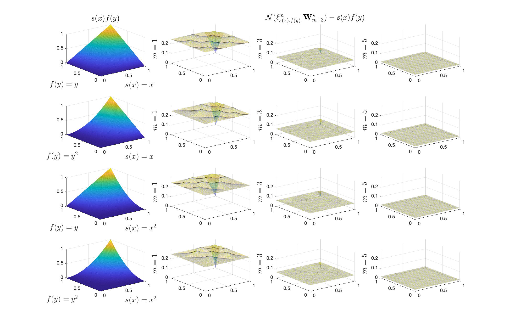
Figure 2: Illustration of Lemma 2.1

Next, we demonstrate Lemma 2.2 using two plots. In Figure 3, we let $r=3$, $\boldsymbol{\alpha}=(a,0,0)^{\top}$, and $\mathbf{x}=(x,1,1)^{\top}$. Therefore, $\mathcal{N}_{\boldsymbol{\ell}^{m}}(\boldsymbol{\ell}_{\mathbf{x}\,|\,{\boldsymbol{\alpha}}}\,|\,\mathbf{W}^{\star}_{m+3})$ should recover $x^{a}$. We thus plot

$$\mathcal{N}_{\boldsymbol{\ell}^{m}}(\boldsymbol{\ell}_{\mathbf{x}\,|\,{\boldsymbol{\alpha}}}\,|\,\mathbf{W}^{\star}_{m+3})-x^{a}\quad\text{for}\quad a\in[3],\ m\in\{1,3,5\}.$$ (5.1)

In Figure 4, we let $r=3$, $\boldsymbol{\alpha}=(a,a,0)^{\top}$, and $\mathbf{x}=(x,y,1)^{\top}$. Therefore, $\mathcal{N}_{\boldsymbol{\ell}^{m}}(\boldsymbol{\ell}_{\mathbf{x}\,|\,{\boldsymbol{\alpha}}}\,|\,\mathbf{W}^{\star}_{m+3})$ should recover $x^{a}y^{a}$. We thus plot

$$\mathcal{N}_{\boldsymbol{\ell}^{m}}(\boldsymbol{\ell}_{\mathbf{x}\,|\,{\boldsymbol{\alpha}}}\,|\,\mathbf{W}^{\star}_{m+3})-x^{a}y^{a}\quad\text{for}\quad a\in[3],\ m\in\{1,3,5\}.$$ (5.2)

Clearly the value of $\mathcal{N}_{\boldsymbol{\ell}^{m}}(\boldsymbol{\ell}_{\mathbf{x}\,|\,{\boldsymbol{\alpha}}}\,|\,\mathbf{W}^{\star}_{m+3})-\mathbf{x}^{\boldsymbol{\alpha}}$ is always non-negative. As $m$ goes up, $\mathcal{N}_{\boldsymbol{\ell}^{m}}(\boldsymbol{\ell}_{\mathbf{x}\,|\,{\boldsymbol{\alpha}}}\,|\,\mathbf{W}^{\star}_{m+3})-\mathbf{x}^{\boldsymbol{\alpha}}$ converges to 0 in each figure from the positive side regardless the value of $a$. Furthermore, it is interesting to see that the differences in both (5.1) and (5.2) actually remain at a constant level, which is only affected by the value of $m$ (i.e., the number of layers of HDNN).

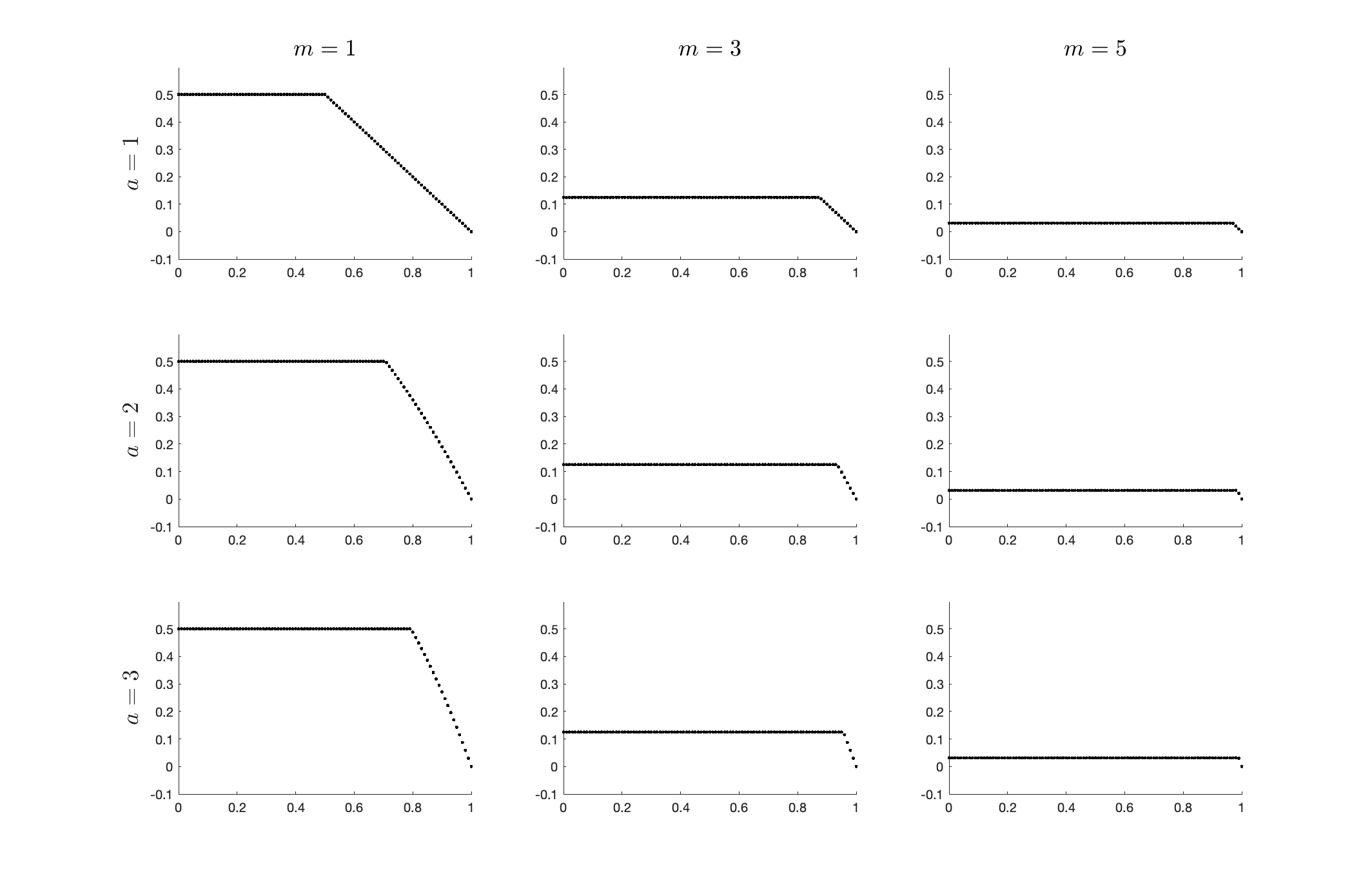
Figure 3: Plots of (5.1)

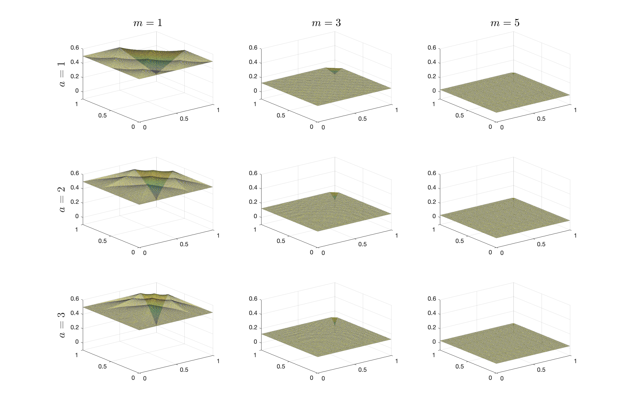
Figure 4: Plots of (5.2)

Finally, we plot $\sigma_{s}(\cdot)$ to justify Lemma 4.1, and let $\phi(\cdot)$ be Epanechnikov kernel (i.e., $\phi(u)=0.75(1-u^{2})I(|u|\leq 1)$) without loss of generality. We first look at the top plot of Figure 5. Here, $\sigma(\cdot)$ is plotted using the black solid line, and GELU (i.e., $\sigma_{G}(u)=u\Phi(u)$ with $\Phi(u)$ being the CDF of $N(0,1)$) is plotted using the magenta solid line. The blue dotted lines stands for $\sigma_{4}(\cdot)$, the cyan dashdot line stands for $\sigma_{8}(\cdot)$, and the red dashed line stands for $\sigma_{16}(\cdot)$. Obviously, $\sigma_{s}(\cdot)$ is able to mimic ReLU in a much better fashion, and the only difference happens at the origin. To see the difference in detail, we zoom in using the bottom plot of Figure 5. It is clear that $\sigma_{s}(\cdot)$ is quite smooth and moves towards $\sigma(\cdot)$ as $s$ increases. More importantly, unlike GELU, $\sigma_{s}(u)$ still acts as a linear term when $u\geq s^{-1}$, so it remains a low computational cost.

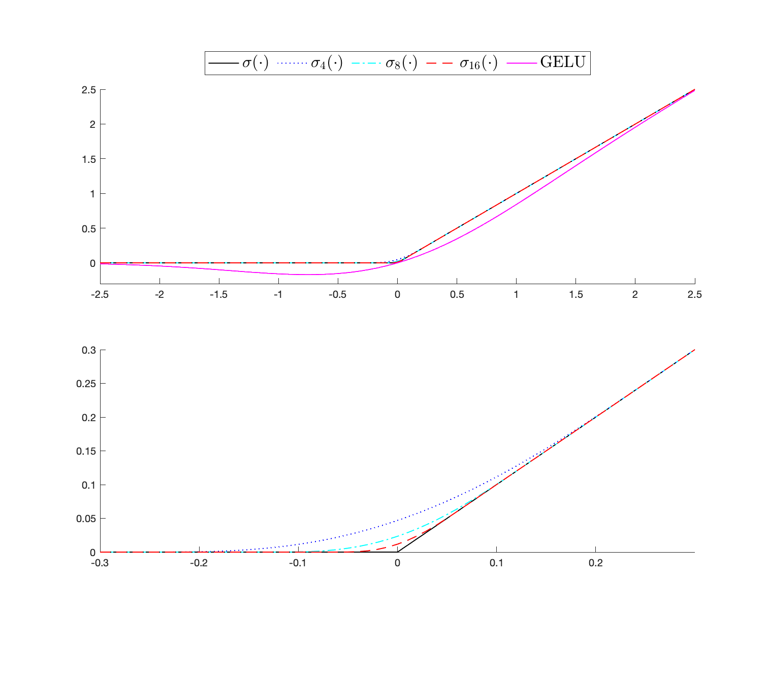
Figure 5: Plots of $\sigma_{s}(\cdot)$

5.2 On Results of Section 3

In this subsection, we conduct simulations to examine the theoretical findings for model (1.2). Specifically, the data generating process is as follows. Let

$$y_{t}=f_{\star}(\mathbf{z}_{1t}^{\top}\,\boldsymbol{\theta}_{\star 1},\ldots,\mathbf{z}_{rt}^{\top}\,\boldsymbol{\theta}_{\star r})+\varepsilon_{t},$$

where $\varepsilon_{t}=\rho_{\varepsilon}\varepsilon_{t-1}+v_{t}$ and $f_{\star}(\mathbf{x})=\frac{2}{r}\left(\sum_{j\text{ is odd}}(5x_{j}+\sin(2x_{j}))+\sum_{j\text{ is even}}\exp(2.5x_{j})\right)$. In the main text, we let $r=2$, and further examine the cases when $r=4,8$ in the supplementary appendix. It is well understood that when $r\geq 4$, a typical nonparametric method such as kernel method will break down. Of course, nothing comes for free. When $r=4,8$, our NN method takes much longer time to compute due to large dimension involved in the calculation.

That said, in what follows, we let

$$\boldsymbol{\theta}_{\star j}=(0.6,0.8)^{\top}\text{ with $j$ being odd},\quad\boldsymbol{\theta}_{\star j}=(0.6,-0.8)^{\top}\text{ with $j$ being even},$$

$$a=0.9,\quad\vartheta=2,\quad z_{it,j}\sim U(-1/1.4,1/1.4),\quad\rho_{\varepsilon}=0.2,$$

where $z_{it,j}$ stands for the $j^{th}$ element of $\mathbf{z}_{it}$. It is easy to know that as we set $a=0.9$, some observations will apparently be left out. Therefore, the design matches the framework of Sections 2 and 3.

For each generated dataset, we conduct estimation as in (3.3). After $J$ replications, we report the following measures:

$$\text{RMSE}_{\boldsymbol{\theta}} = \left\{\frac{1}{J}\sum_{j=1}^{J}\|\widehat{\boldsymbol{\theta}}_{j}-\boldsymbol{\theta}_{\star}\|^{2}\right\}^{1/2},$$

$$\text{RMSE}_{f} = \left\{\frac{1}{JL}\sum_{j=1}^{J}\sum_{l=1}^{L}\|\widehat{f}_{j}(\mathbf{x}_{l})-f_{\star}(\mathbf{x}_{l})\|^{2}\right\}^{1/2},$$

$$\text{CR}_{\boldsymbol{\theta}} = \frac{1}{Jd}\sum_{j=1}^{J}\sum_{s=1}^{d}I[(\widehat{\theta}_{j,s}-\theta_{\star,s})\in\text{CI}_{j,s}],$$

where $\widehat{\boldsymbol{\theta}}_{j}$ and $\widehat{f}_{j}(\cdot)$ stand for the estimates of $\boldsymbol{\theta}_{\star}$ and $f_{\star}(\cdot)$ in the $j^{th}$ replication, and $\widehat{\theta}_{j,s}$ and $\theta_{\star,s}$ are the $s^{th}$ elements of $\widehat{\boldsymbol{\theta}}_{j}$ and $\boldsymbol{\theta}_{\star}$. In addition, $\text{CI}_{j,s}$ is the 95% confidence interval for the $s^{th}$ element in the $j^{th}$ replication based on the bootstrap draws, and $\{\mathbf{x}_{l}\,|\,l\in 0\cup[L]\}$ are some pre-determined points: $\mathbf{x}_{l}=(-a+l\cdot 2a/L)\mathbf{1}_{r}.$ To implement the bootstrap procedure, we choose the Bartlett kernel (i.e., $y=(1-|x|)I(|x|\leq 1)$), and follow the suggestion from such as Palm et al. (2011) to let $\ell=\lfloor 1.75T^{1/3}\rfloor$ for simplicity. We limit the number of bootstrap replications to 100 due to time and computation constraints. Also we let $T\in\{500,1000,2000\}$, $h\asymp T^{-1/4}$, and $m\in\{3,4,5\}$, where $m$ controls the number of layers of in each hierarchy. Finally, to exam our argument under Lemma 4.1 we also repeat the above procedure using $\sigma_{s}(\cdot)$ by letting $s=32$, so $\sigma_{s}(\cdot)$ is sufficiently close to $\sigma(\cdot)$, and is smooth.

Table 1: RMSE and Coverage Rate ($r=2$)

		RMSE (via $\sigma$)				RMSE (via $\sigma_{s}$)
	$T$	$m=3$	$m=4$	$m=5$		$m=3$	$m=4$	$m=5$
$\text{RMSE}_{\boldsymbol{\theta}}$	500	0.0212	0.0187	0.0177		0.0169	0.0142	0.0162
	1000	0.0134	0.0137	0.0128		0.0101	0.0094	0.0078
	2000	0.0097	0.0097	0.0092		0.0087	0.0076	0.0084
$\text{RMSE}_{f}$	500	0.3929	0.4009	0.3969		0.4033	0.4396	0.3639
	1000	0.2823	0.2765	0.2744		0.2636	0.2624	0.2681
	2000	0.2003	0.2015	0.2000		0.1863	0.1839	0.1856
	Coverage Rate
$\text{CR}_{\boldsymbol{\theta}}$	500	0.8875	0.9125	0.9150		0.8850	0.8750	0.9375
	1000	0.9075	0.9225	0.9400		0.9075	0.9250	0.9550
	2000	0.9275	0.9325	0.9375		0.9125	0.9600	0.9500

We summarize the results of $r=2$ in Table 1 and provide the results of $r=4,8$ in Table B1 of the supplementary appendix. As shown in Table 1, it is clear that both $\text{RMSE}_{\boldsymbol{\theta}}$ and $\text{RMSE}_{f}$ converge to 0, and $\text{RMSE}_{\boldsymbol{\theta}}$ converges at a much faster rate. It is not surprising, as $\widehat{\boldsymbol{\theta}}$ enjoys a parametric rate. Additionally, we see that as the sample size goes up, $\text{CR}_{\boldsymbol{\theta}}$ converges to 95% which is the nominal rate. Overall, $m=5$ offers better finite sample performance, which is also consistent with the finding of Section 5.1. Due to the complexity of DNN and the slow rate of $\text{RMSE}_{f}$, we need reasonably large sample size, which is also required by some of the existing simulation designs using i.i.d. data (e.g., Du et al., 2021; Farrell et al., 2021). Last but not least, we see $\sigma_{s}(\cdot)$ and $\sigma(\cdot)$ offer equivalent finite sample performance. Although we see differences in the third digits, but in view of the number of replications of Monte Carlo design, we should not emphasize these differences too much. Again, to understand the differences between $\sigma_{s}(\cdot)$ and $\sigma(\cdot)$, one should conduct a systematic comparison as in Hendrycks and Gimpel (2023).

5.3 An Empirical Study

In this subsection, we examine the bond return predictability. Understanding the predictability of bond returns has always been a central topic in finance (e.g., Ludvigson and Ng, 2009; Andreasen et al., 2020; Borup et al., 2023). The literature seems to agree that excess bond returns are forecastable by financial indicators such as yield spreads (Andreasen et al., 2020), while also acknowledges the nonlinearity from modelling perspective (Borup et al., 2023). In addition, to avoid variable selection problem, one often conducts principal component analysis (PCA) to collect some key factors from a large group of macro variables to be the key predictors of the forecasting model (Ludvigson and Ng, 2009). The above features naturally fit our example of Section 4.

We consider two benchmark models in this section:

$$y_{t+1} = a+\varepsilon_{t+1},$$ (5.3)

$$y_{t+1} = a+\mathbf{x}_{t}^{\top}\boldsymbol{\beta}+\varepsilon_{t+1},$$ (5.4)

where $y_{t+1}$ denotes the 1-month log excess holding period return on a 2-month zero-coupon treasury bond. Here (5.3) is a simple constant mean model, while (5.4) is a typical one step ahead linear model including some key predictors. Specifically, $\mathbf{x}_{t}$ includes a set of variables adopted in Borup et al. (2023) and covers the period from December 1961 to December 2018: 1) yields spreads computed as the difference between the yield on a bond with 2 months to maturity and the implied yield on a one-month treasury bill obtained from CRSP; 2) forward spreads computed as the difference between the 2-month forward rate and the one-month yield; 3) the first principal component (PC) of yields obtained using 12, 24, 36, 48, and 60 month yields; 4) a linear combination of forward rates obtained from projecting 12, 24, 36, 48, and 60 month forward rates onto the mean excess bond return across the maturity spectrum; and 5) a linear combination of macroeconomic factors obtained using the FRED-MD database and estimated analogously to CP. As the first two predictors are observed, they form $\mathbf{z}_{1t}$. The last three predictors are obtained from estimation, so they form $\mathbf{z}_{2t}$ as specified in Example 1 of Section 1.

Having the dataset ready, we first partition the data into a training set $S_{tr}$ (data from 1961 to 2011) and a test set $S_{te}$ (data from 2012 and 2018) (referred to as Partition I). For each model, we run regression using training set only to obtain the parameter estimates, and calculate $\widehat{y}_{t}$ for the test set. For the DNN approach, we also let $m=3,4,5$ to examine the impact of different layers practically.

To evaluate the performance of different methods, we calculate

$$\text{RMSE}=\left\{\frac{1}{\sharp S_{te}}\sum_{t\in S_{te}}(\widehat{y}_{t}-y_{t})^{2}\right\}^{1/2}\quad\text{and}\quad\text{CS}=\frac{1}{\sharp S_{te}}\sum_{t\in S_{te}}I(\widehat{y}_{t}\cdot y_{t}>0),$$ (5.5)

where $\sharp S_{te}$ stands for the cardinality of $S_{te}$. The first measure is a typical root mean squared errors based on the test set, and the second measure examines the sign prediction and reports the percentage of correct sign prediction. There is a vast literature regarding sign prediction (e.g., Christoffersen and Diebold, 2006; Nyberg, 2011), which argues that return is not predictable in general, but one can forecast the sign of return much better. Although predicting the sign is not the focus of the paper, it is interesting to see how DNN performs practically along this line of research.

Alternatively, we consider a rolling window idea to partition the data (referred to as Partition II). The window size is always 50 years. For each window, we run regression using each model, and then use the estimated parameters to forecast the following year (i.e., the test set always includes data of one year). Again, we report RMSE and CS based on our forecasts.

Table 2: RMSE and CS

		Model (5.3)	Model (5.4)	DNN
				$m=3$	$m=4$	$m=5$
Partition I	RMSE	0.2267	0.2209	0.2138	0.2047	0.2098
	CS	0.5833	0.5833	0.5952	0.6429	0.6905
Partition II	RMSE	0.2274	0.2195	0.2025	0.2002	0.2095
	CS	0.5833	0.5833	0.6905	0.5952	0.6429

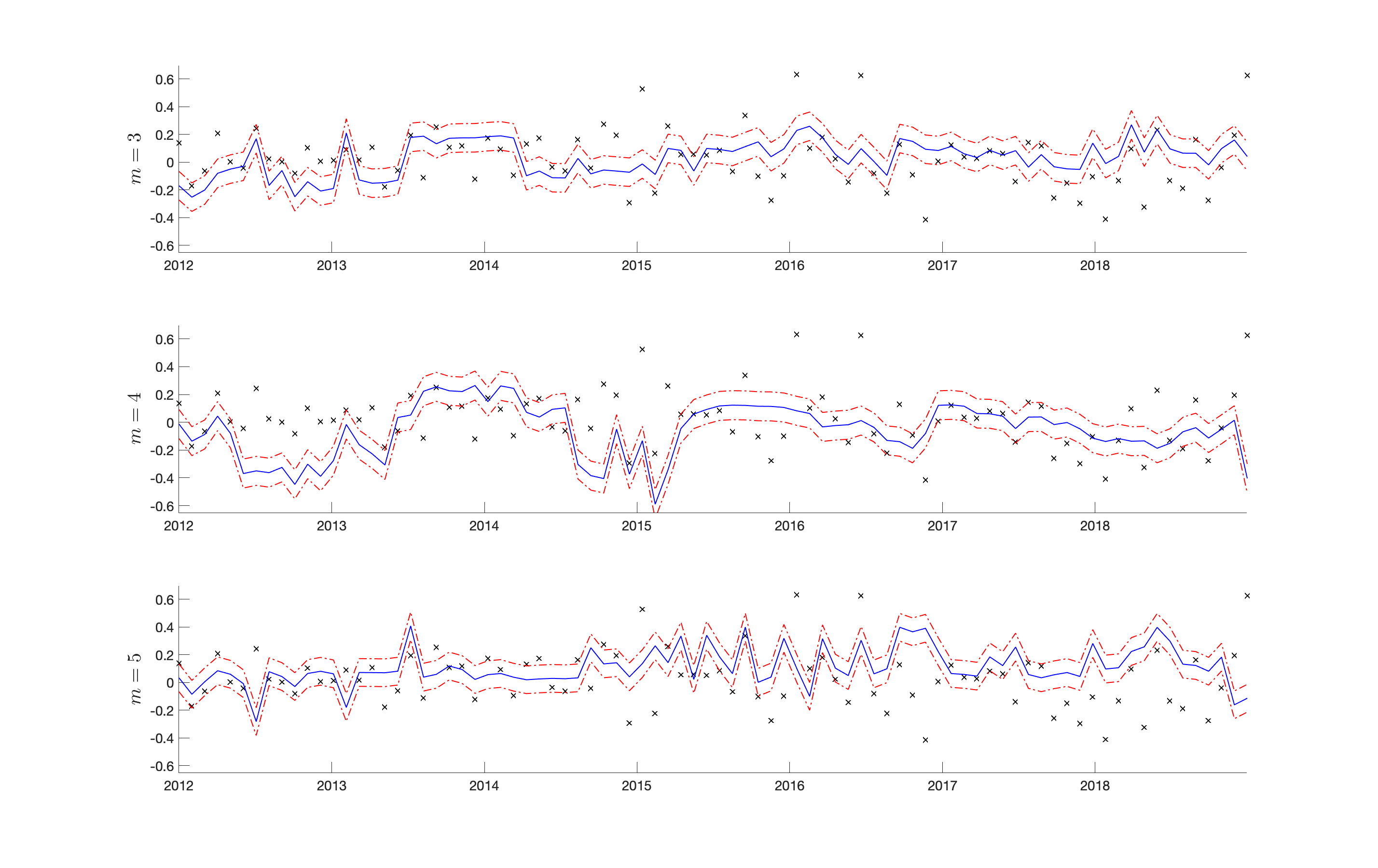
Figure 6: Examination using Test Set

We summarize the results in Table 2. As shown in the table, DNN approach in general outperforms Model (5.3) and Model (5.4) in terms of both RMSE and CS. Here, smaller RMSE implies less forecast errors, while higher CS means better sign prediction. To further see the differences when using different layers (i.e., $m=3,4,5$) for DNN approach, we plot the point forecasts and their confidence intervals using Partition I for example in Figure 6. In the figure, the actual $y_{t}$’s are marked using “x”, the estimated values are represented using blue solid lines, and the red dotted-hash lines stand for the 95% confidence intervals. When $m=5$, DNN approach seems to offer a better coverage for the period from 2012 to 2015, while for the period from 2016 to 2018, it is quite hard to cover all the points regardless the value of $m$. This finding is consistent with Borup et al. (2023), in which the authors argue that the predictability varies with respect to time and economic conditions. Certainly, one may conduct a more comprehensive investigation as in the literature, and we do not pursue these results further in order not to deviate from our main goal.

6 Conclusion with Discussion

Before concluding, we provide a few useful remarks.

On the Design of DNN — Note that we require $f_{\star}(\mathbf{x})$ to be defined on a compact set, but do not impose restriction on the range of $\{\mathbf{z}_{t}\}$. In fact, for time series data, it may make more sense to assume that $a$ is diverging, which is indeed achievable. Suppose that $\mathbf{z}_{t}$ follows a sub-Gaussian distribution. In this case, after some algebra we can relax the condition on $a$ to $\sqrt{\log(Th^{r})}\cdot a\to\infty.$ Apparently, there is a price that we have to pay, which is the slow rate of convergence. A similar treatment has also been discussed in Li et al. (2016) for example, so we do not further elaborate it here.

The total number of layers that we require for Theorem 2.1 is

$$\left\{\begin{array}[]{ll}(m+3)\cdot\lceil\log_{2}r\rceil&\text{for }r\geq 2\\ m+3&\text{for }r=1\end{array}\right..$$

The width of most layers in the hierarchy is 6. The sparsity occurs naturally in view of Definition 2.1 and Lemma 2.1.

Connection with Some Existing Studies — Recently, Du et al. (2021) and Farrell et al. (2021) apply DNN to study treatment effects using micro datasets, and Keane and Neal (2020) apply DNN to study climate data. Our research can be extended to related topics, and our analysis provides a numerical implementation perspective that complements existing studies. Specifically, we have a clear understanding of the minimization process.

To conclude, we consider the estimation of both the multi-index parameters and the link function involved in a class of semiparametric DNN models. We contribute to the design of DNN by i) providing more transparency for practical implementation, ii) defining different types of sparsity, iii) showing the differentiability, iv) pointing out the set of effective parameters, and v) offering a new variant of rectified linear activation function (ReLU), etc. The model setup also sheds light on how to generalize factor augmented models that are of practical significance. The asymptotic properties of the proposed estimates are derived accordingly, and they can be applied to a wide class of non– and semi–parametric models. Finally, we conduct extensive numerical studies to examine the theoretical findings.

Appendix A Notation & Preliminary Lemmas

In this appendix, we first introduce extra notations which will be repeatedly used in the development, and then present the preliminary lemmas.

Throughout, we let $I_{\mathbf{i}}(\mathbf{x})=I(\mathbf{x}\in C_{\mathbf{x}_{\mathbf{i}}}),$ where $C_{\mathbf{x}_{\mathbf{i}}}$ is defined in (2.3). For $\forall k\in\mathbb{N}$, denote a mapping $T^{k}:[0,2^{2-2k}]\mapsto[0,2^{-2k}]$ as follows:

$$T^{k}(x)=\frac{x}{2}\wedge\left(2^{1-2k}-\frac{x}{2}\right).$$ (A.1)

To see the validity of (A.1), we write

$$T^{k}(x) = \frac{x}{2}+0\wedge\left(2^{1-2k}-x\right)$$ (A.2)

$$= \frac{x}{2}-0\vee\left(x-2^{1-2k}\right)$$

$$= \sigma\left(\frac{x}{2}\right)-\sigma\left(x-2^{1-2k}\right),$$

where the third equality follows from the fact that $\sigma\left(\frac{x}{2}\right)=\frac{x}{2}$ because of $x$ being defined on $[0,2^{2-2k}]$. In view of (A.2), we partition $[0,2^{2-2k}]$ as $[0,2^{1-2k}]\cup[2^{1-2k},2^{2-2k}]$, and immediately obtain that

$$T^{k}(x)=\left\{\begin{array}[]{ll}\frac{1}{2}x&\text{for }x\in[0,2^{1-2k}]\\ 2^{1-2k}-\frac{1}{2}x&\text{for }x\in[2^{1-2k},2^{2-2k}]\end{array}\right.,$$

of which either expression on the right hand side fulfils $T^{k}(x)\in[0,2^{-2k}]$. Thus, we conclude $T^{k}:[0,2^{2-2k}]\to[0,2^{-2k}]$.

We then define $R^{k}:[0,1]\mapsto[0,2^{-2k}]$ as follows:

$$R^{k}(x)=T^{k}\circ T^{k-1}\circ\cdots\circ T^{1}(x),$$ (A.4)

and let further $\mathbf{R}_{m}(x)=(R^{1}(x),\ldots,R^{m}(x))^{\top}$. In Figure 7, we plot $R^{k}(x)$ with $k\in[4]$ for the purpose of demonstration. It is easy to see that $R^{k}(x)$ is piece wise linear, and the value of $R^{k}(x)$ shrinks towards 0 as $k$ increases.

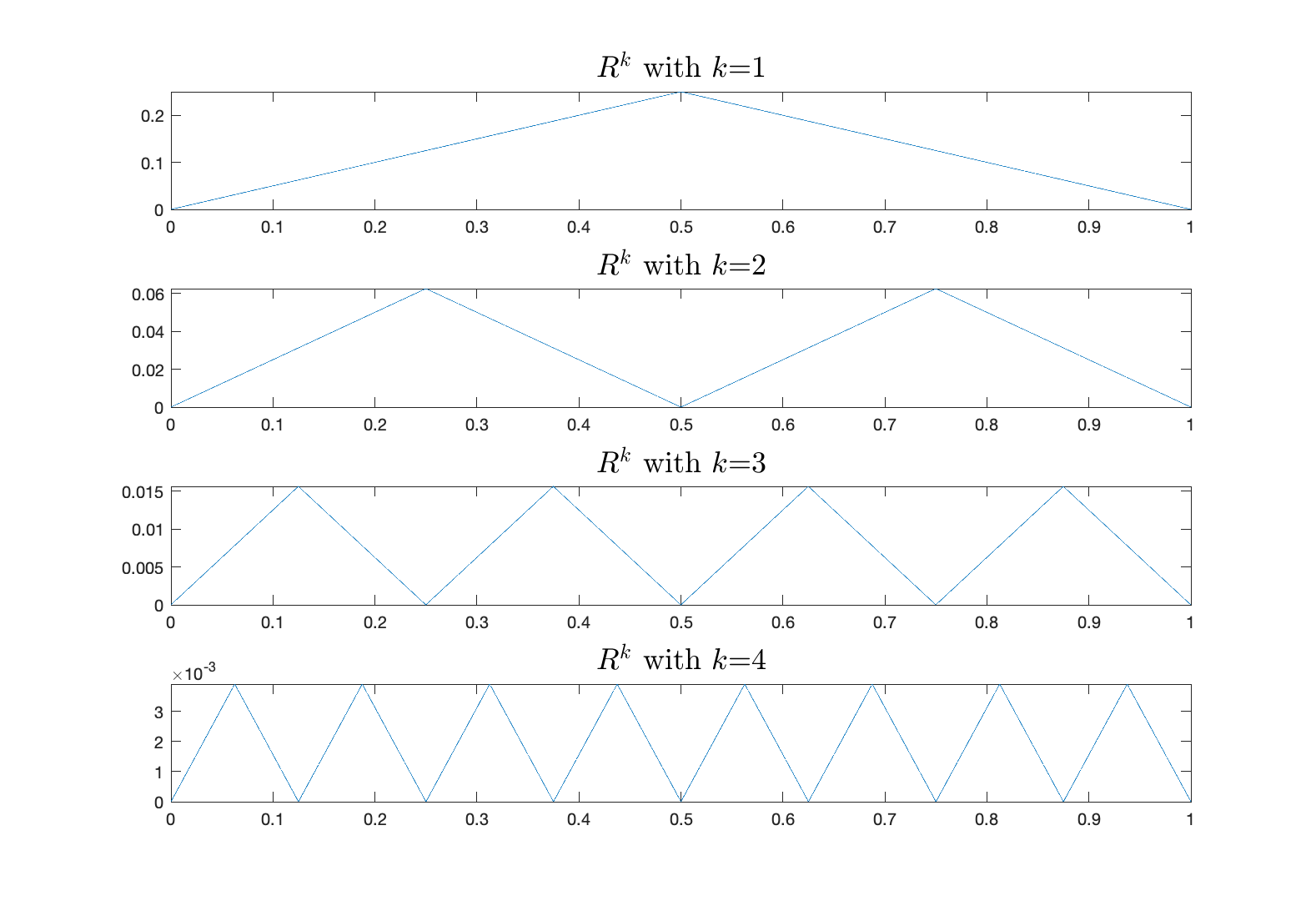
Figure 7: Plots of $R^{k}(x)$ with $k\in[4]$

Next, we provide a few preliminary lemmas.

Lemma A1.

Let $f\,:\,[-a,a]^{r}\to\mathbb{R}$ be a $(p,\mathscr{C})$-smooth function, where $p=\vartheta+s$. For $\forall\mathbf{x}_{0}\in[-a,a]^{r}$, let

$$p_{\vartheta}(\mathbf{x}\,|\,\mathbf{x}_{0})=\sum_{\|\mathbf{J}\|_{1}\leq\vartheta}\frac{1}{\mathbf{J}!}f^{(\mathbf{J})}(\mathbf{x}_{0})(\mathbf{x}-\mathbf{x}_{0})^{\mathbf{J}}.$$

Then for $\forall\boldsymbol{\delta}=(\delta_{1},\ldots,\delta_{r})^{\top}$ satisfying $\|\boldsymbol{\delta}\|_{1}\leq\vartheta$,

$$\|f^{(\boldsymbol{\delta})}(\mathbf{x})-p_{\vartheta}^{(\boldsymbol{\delta})}(\mathbf{x}\,|\,\mathbf{x}_{0})\|_{\infty}^{[-a,a]^{r}}\leq O(1)\|\|\mathbf{x}-\mathbf{x}_{0}\|^{p-\|\boldsymbol{\delta}\|_{1}}\|_{\infty}^{[-a,a]^{r}},$$

where $O(1)$ depends on $r$ and $\vartheta$ only.

Lemma A2.

For $\forall m\in\mathbb{N}$, $\|\mathbf{R}_{m}(x)\|_{1}$ admits a DNN representation:

$$\|\mathbf{R}_{m}(x)\|_{1} = \mathbf{w}_{\operatorname*{\text{out}}}^{\top}\boldsymbol{\sigma}_{\widetilde{\mathbf{v}}_{m}}\widetilde{\mathbf{w}}\,\boldsymbol{\sigma}_{\widetilde{\mathbf{v}}_{m-1}}\cdots\widetilde{\mathbf{w}}\,\boldsymbol{\sigma}_{\widetilde{\mathbf{v}}_{1}}(\mathbf{w}_{\operatorname*{\text{in}}}\cdot x):=\operatorname*{\mathcal{N}}(\mathbf{w}_{\operatorname*{\text{in}}}\cdot x\,|\,\mathbf{W}_{\mathbf{R}_{m}}),$$

where $\widetilde{\mathbf{w}}$ is defined in Lemma 2.1 already,

$$\mathbf{w}_{\operatorname*{\text{in}}}=\begin{pmatrix}\frac{1}{2}\\ 1\\ 0\end{pmatrix},\quad\mathbf{w}_{\operatorname*{\text{out}}}=\begin{pmatrix}1\\ -1\\ 1\end{pmatrix},\quad\text{and}\quad\widetilde{\mathbf{v}}_{k}=\begin{pmatrix}0\\ 2^{1-2k}\\ 0\end{pmatrix}\text{ for $k\in[m]$}.$$

According to Definition 1.1, the value of $\mathbf{W}_{\mathbf{R}_{m}}$ is obvious. It is noteworthy that $\widetilde{\mathbf{w}}$ is a $3\times 3$ square matrix, but only has rank 2.

Lemma A3.

For $\forall m\in\mathbb{N}$, $\|\mathbf{R}_{m}(x)\|_{1}$ is Lipschitz continuous on $[0,1]$, and is piecewise linear on the following intervals:

$$[\ell\cdot 2^{-m},(\ell+1)\cdot 2^{-m})\text{ for }\ell=0\cup[2^{m}-2],$$

$$[\ell\cdot 2^{-m},(\ell+1)\cdot 2^{-m}]\text{ for }\ell=2^{m}-1.$$

Let $\frac{\partial(\|\mathbf{R}_{m}(x)\|_{1})}{\partial x}$ be defined accordingly. Then we obtain that

1. $\|g(x)-\|\mathbf{R}_{m}(x)\|_{1}\|_{\infty}^{[0,1]}\leq 2^{-m}$,

2. $\left\|\frac{\partial(\|\mathbf{R}_{m}(x)\|_{1})}{\partial x}-\frac{\partial g(x)}{\partial x}\right\|_{\infty}^{[0,1]}\leq 2^{-m+1}$,

where $g(x)=x(1-x)$.

In Figure 8, we give some plots to illustrate our statements in Lemma A3. The difference between $\|\mathbf{R}_{m}(x)\|_{1}$ and $g(x)$ becomes visually negligible when $m\geq 3$.

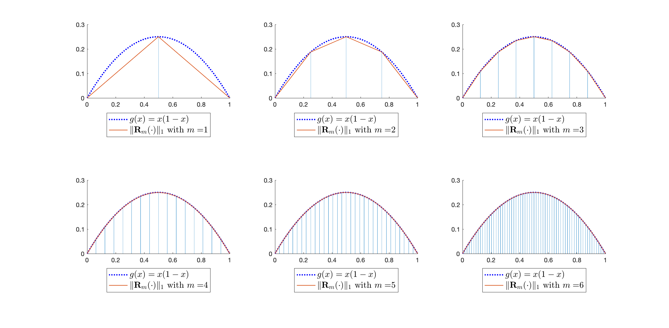
Figure 8: Illustration of Lemma A3

We now recall the mapping $\boldsymbol{\ell}_{\mathbf{x}\,|\,\boldsymbol{\alpha}}$ defined in the end of Section 1, which gives

$$\boldsymbol{\ell}_{\mathbf{x}\,|\,{\mathbf{1}_{r}}}=(\mathbf{x}^{\top},\mathbf{1}_{q}^{\top})^{\top}\quad\text{with}\quad q=\left\{\begin{array}[]{ll}2^{\lceil\log_{2}r\rceil}-r&\text{for }r\geq 2\\ 1&\text{for }r=1\end{array}\right..$$ (A.7)

We are then able to present the following lemma.

Lemma A4.

Using $\operatorname*{\mathcal{N}}(\boldsymbol{\ell}^{m}_{x,y}\,|\,\mathbf{W}^{\star}_{m+3})$ of Lemma 2.1, define $\mathcal{N}_{\boldsymbol{\ell}^{m}}(\boldsymbol{\ell}_{\mathbf{x}\,|\,{\mathbf{1}_{r}}}\,|\,\mathbf{W}^{\star}_{m+3})$ according to Definition 2.1, where $r\geq 2$, $\mathbf{x}\in[0,h]^{r}$, and $h\leq 1-\lceil\log_{2}r\rceil\cdot 2^{-m}$. Then the following results hold:

1. $0\leq\mathcal{N}_{\boldsymbol{\ell}^{m}}(\boldsymbol{\ell}_{\mathbf{x}\,|\,{\mathbf{1}_{r}}}\,|\,\mathbf{W}^{\star}_{m+3})\leq 1$ uniformly on $[0,h]^{r}$,

2. $0\leq\mathcal{N}_{\boldsymbol{\ell}^{m}}(\boldsymbol{\ell}_{\mathbf{x}\,|\,{\mathbf{1}_{r}}}\,|\,\mathbf{W}^{\star}_{m+3})-\mathbf{x}^{\mathbf{1}_{r}}\leq 3^{\lceil\log_{2}r\rceil-1}2^{-m}$ uniformly on $[0,h]^{r}$,

3. $\|\frac{\partial}{\partial x_{i}}[\mathcal{N}_{\boldsymbol{\ell}^{m}}(\boldsymbol{\ell}_{\mathbf{x}\,|\,{\mathbf{1}_{r}}}\,|\,\mathbf{W}^{\star}_{m+3})-\mathbf{x}^{\mathbf{1}_{r}}]\|_{\infty}^{[0,h]^{r}}\leq 3^{\lceil\log_{2}r\rceil-1}2^{-m}$ for $\forall i\in[r]$.

Lemma A5.

Suppose that $\boldsymbol{\Sigma}_{11}+\boldsymbol{\Sigma}_{12}+\boldsymbol{\Sigma}_{12}^{\top}$ is positive definite, where $\boldsymbol{\Sigma}_{11}$ and $\boldsymbol{\Sigma}_{12}$ are defined in Theorem 3.1. Under Assumptions 1-2, as $(h,Th^{r})\to(0,\infty)$,

1. $\frac{1}{\sqrt{T}}\sum_{t=1}^{T}\varepsilon_{t}\,\mathbf{f}^{(1)}_{\star}(\mathbf{z}_{t}\,\boldsymbol{\theta}_{\star})\,\widetilde{\mathbf{z}}_{t}I_{a,t}\to_{D}N(\mathbf{0},\boldsymbol{\Sigma}_{11}+\boldsymbol{\Sigma}_{12}+\boldsymbol{\Sigma}_{12}^{\top})$,

2. for $\forall\mathbf{x_{0}}\in[-a,a]^{r}$, $\frac{1}{\sqrt{Th^{r}}}\sum_{t=1}^{T}\sum_{\mathbf{i}\in[M]^{2}}\varepsilon_{t}I_{\mathbf{i},t,\mathbf{x}_{0}}\mathbf{H}^{-1}\boldsymbol{\psi}_{r_{\vartheta}}(\mathbf{z}_{t}\,\boldsymbol{\theta}_{\star}\,|\,\mathbf{x}_{\mathbf{i}})\to_{D}N(\mathbf{0},\boldsymbol{\Sigma}_{2,\mathbf{x}_{0}})$,

where $I_{\mathbf{i},t,\mathbf{x}_{0}}=I(\mathbf{x}_{0}\in C_{\mathbf{x}_{\mathbf{i}}})I_{\mathbf{i}}(\mathbf{z}_{t}\,\boldsymbol{\theta}_{\star})$ and $\boldsymbol{\Sigma}_{2,\mathbf{x}_{0}}=\sigma_{\varepsilon}^{2}\phi_{\boldsymbol{\theta}_{\star}}(\mathbf{x}_{0})\int_{[0,1]^{r}}\boldsymbol{\psi}_{r_{\vartheta}}(\mathbf{w})\boldsymbol{\psi}_{r_{\vartheta}}(\mathbf{w})^{\top}\mathrm{d}\mathbf{w}.$

In the appendices, we first provide some extra plots and simulation results in B1, and then give the proofs in Appendix B2.

Appendix B1 Extra Numerical Results

B1.1 Extra Plots

In this appendix, we provide some extra plots using $\sigma_{s}(\cdot)$. As in Figure 2 of the main text, we show that Lemma 2.1 still holds when $\sigma_{s}(\cdot)$ is adopted. The setting is the same as those in Figure 2, but we replace $\sigma(\cdot)$ with $\sigma_{s}(\cdot)$ in which $s=16,\,32$, and $\phi(\cdot)$ is chosen to be Epanechnikov kernel (i.e., $\phi(u)=0.75(1-u^{2})I(|u|\leq 1)$) without loss of generality.

As shown in Figure 2, Figures B2 and B2, the differences are overall at the same magnitude, and they all shrink towards 0 as $m$ increases. As $s$ increases, the differences of Figure B2 look more similar to those presented in 2.

In addition, we replot (5.1) and (5.2) of the main text using using $\sigma_{s}(\cdot)$. Again, we replace $\sigma(\cdot)$ with $\sigma_{s}(\cdot)$ in which $s=16,\,32$, and $\phi(\cdot)$ is chosen to be Epanechnikov kernel. The findings are almost the same as aforementioned. As $s$ increases, the differences in Figures B4 and B6 very much similar to those in Figures 3 and 4 of the main text. It is worth mentioning that in Figure 3, there are some obvious non–smooth changing points, which become much smoother in Figures B4 and B4 due to the use of $\sigma_{s}(\cdot)$.

Overall, we can conclude that the main results developed in Sections 2 and 3 remain valid by replacing $\sigma(\cdot)$ with $\sigma_{s}(\cdot)$.

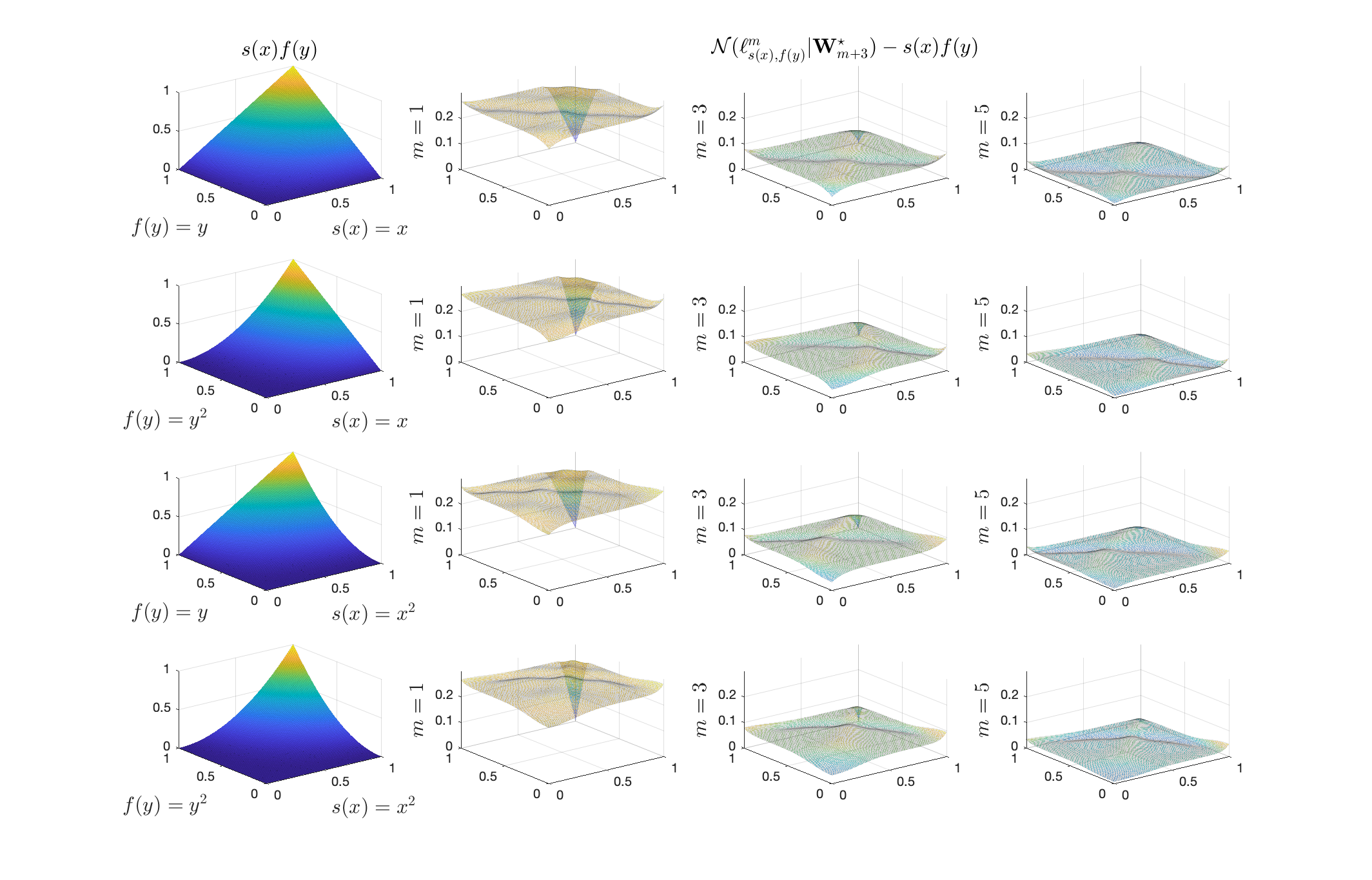
Figure B1: Illustration of Lemma 2.1 using $\sigma_{16}(\cdot)$

Figure B2: Illustration of Lemma 2.1 using $\sigma_{32}(\cdot)$

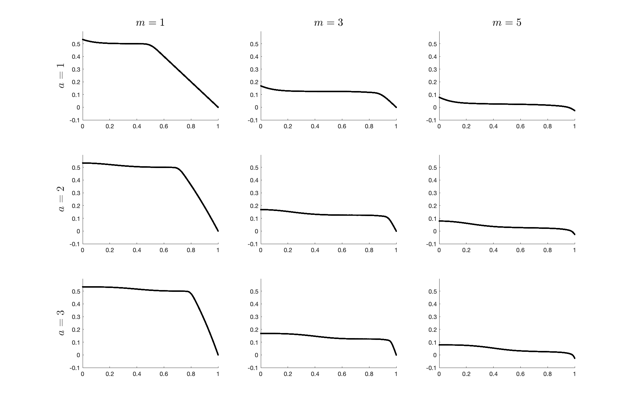
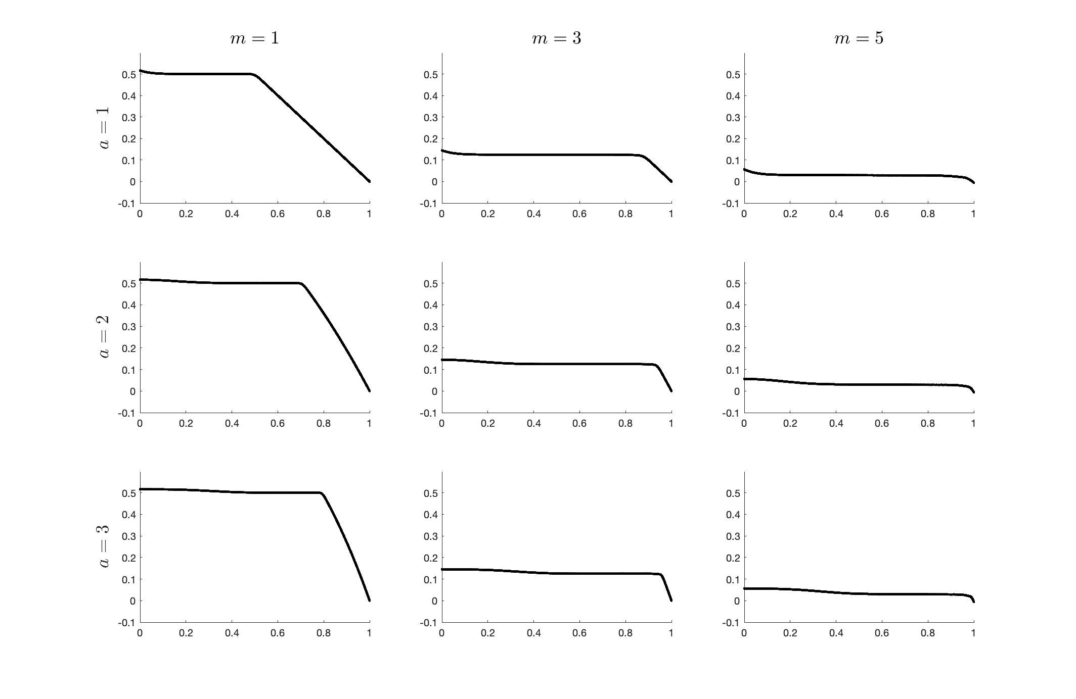
Figure B3: Plots of (5.1) using $\sigma_{16}(\cdot)$

Figure B4: Plots of (5.1) using $\sigma_{32}(\cdot)$

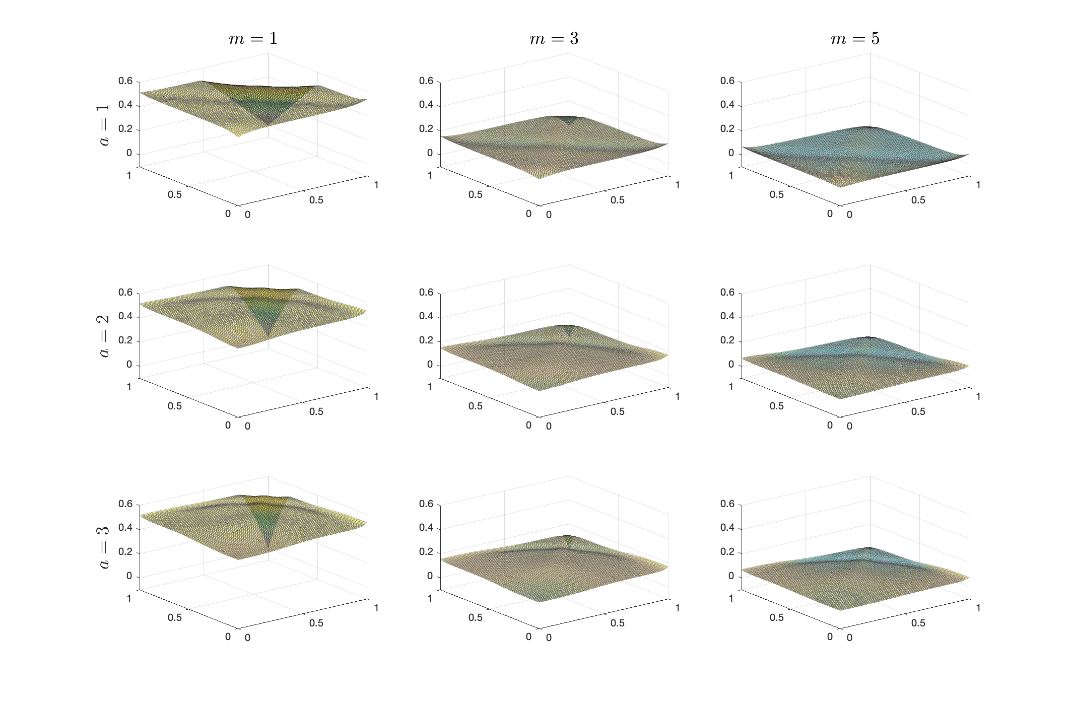
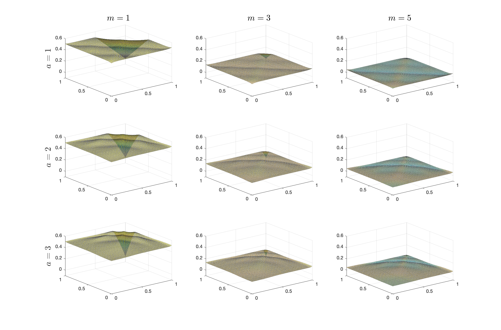
Figure B5: Plots of (5.2) using $\sigma_{16}(\cdot)$

Figure B6: Plots of (5.2) using $\sigma_{32}(\cdot)$

B1.2 Simulation Results with Large $r$

As mentioned in the main text, it is well understood that when $r\geq 4$, a typical nonparametric method such as kernel method will break down. Of course, nothing comes for free. When $r=4,8$, our NN method takes much longer time to compute due to large dimension involved in the calculation. Take $r=8$ for example, it takes a few hours to get one estimation done for $T\in\{1000,2000\}$. As a result, it is impossible for us to calculate coverage rates using bootstrap method plus a large number of simulation replications. In practice, as one does not need to repeatedly implement the bootstrap draws, calculating confidence interval is still feasible. That said, in what follows, we focus on bias and standard deviation, which are the focus of majority of DNN based studies anyway. Therefore, the following numerical results do not lose any generality.

Majority notations and quantities have been introduced in the main text. We present some new notations and measures below:

$$\text{Bias}_{\boldsymbol{\theta}} = \frac{1}{J}\sum_{j=1}^{J}\|\widehat{\boldsymbol{\theta}}_{j}-\boldsymbol{\theta}_{\star}\|_{2}/r,$$

$$\text{Bias}_{f} = \frac{1}{JL}\sum_{j=1}^{J}\sum_{l=1}^{L}|\widehat{f}_{j}(\mathbf{x}_{l})-f_{\star}(\mathbf{x}_{l})|,$$

$$\text{Std}_{\boldsymbol{\theta}} = \left\{\frac{1}{J}\sum_{j=1}^{J}\|\widehat{\boldsymbol{\theta}}_{j}-\overline{\boldsymbol{\theta}}\|_{2}/r\right\}^{1/2},$$

$$\text{Std}_{f} = \left\{\frac{1}{JL}\sum_{j=1}^{J}\sum_{l=1}^{L}|\widehat{f}_{j}(\mathbf{x}_{l})-\overline{f}_{j}(\mathbf{x}_{l})|\right\}^{1/2},$$ (B1.1)

where $\overline{\boldsymbol{\theta}}=\frac{1}{J}\sum_{j=1}^{J}\widehat{\boldsymbol{\theta}}_{j}$ and $\overline{f}_{j}(\mathbf{x}_{l})=\frac{1}{J}\sum_{j=1}^{J}\widehat{f}_{j}(\mathbf{x}_{l})$. Here $\mathbf{x}_{l}$’s are selected in the same way as in the main text. Note that ideally, we would like to select say 10 points on each dimension of $\mathbf{x}$ when evaluating the performance of $\widehat{f}$. However, it is not feasible practically, because $10^{r}$ with $r=8$ requires us to evaluate an extreme large number of points just for one simulation replication, which will definitely create lots of computation burden.

We summarize the results in Table B1. As we can see, the method presented in the paper still provides reasonable finite sample performance when $r=4,8$. A few facts emerge: (1). It seems that $\text{Bias}_{\boldsymbol{\theta}}$ has less bias via $\sigma(\cdot)$, and $\text{Std}_{\boldsymbol{\theta}}$ is smaller via $\sigma_{32}(\cdot)$. Thus, introducing $\sigma_{s}$ seems to be balancing bias and standard deviation if we just focus on the estimate of $\boldsymbol{\theta}_{\star}$. (2). The same pattern can be found for the estimate of $f_{\star}$. In this case, the biases associated with $\sigma_{32}(\cdot)$ seem to be much larger, but they do not increase much when $r$ changes from 4 to 8. (3) $m$ does not seem to play any serious role over all.

Table B1: Extra Simulation Results

				Bias			Std
			$T$	$m=3$	$m=4$	$m=5$	$m=3$	$m=4$	$m=5$
$r=4$	via $\sigma(\cdot)$	$\boldsymbol{\theta}$	500	0.0103	0.0080	0.0062	0.0305	0.0309	0.0323
			1000	0.0086	0.0072	0.0099	0.0222	0.0211	0.0213
			2000	0.0082	0.0085	0.0114	0.0147	0.0150	0.0154
		$f$	500	0.2450	0.2646	0.2694	0.3285	0.3289	0.3355
			1000	0.2528	0.2616	0.2571	0.2328	0.2281	0.2424
			2000	0.2647	0.2675	0.2630	0.1690	0.1598	0.1538
	via $\sigma_{32}(\cdot)$	$\boldsymbol{\theta}$	500	0.0042	0.0072	0.0033	0.0392	0.0477	0.0495
			1000	0.0044	0.0029	0.0016	0.0385	0.0385	0.0326
			2000	0.0016	0.0027	0.0047	0.0296	0.0307	0.0322
		$f$	500	0.6926	0.7338	0.5831	0.2821	0.2696	0.3010
			1000	0.6816	0.7352	0.5956	0.2151	0.1882	0.2048
			2000	0.6821	0.7259	0.5892	0.1409	0.1446	0.1352
$r=8$	via $\sigma(\cdot)$	$\boldsymbol{\theta}$	500	0.0114	0.0088	0.0100	0.0630	0.0655	0.0625
			1000	0.0108	0.0085	0.0115	0.0436	0.0445	0.0429
			2000	0.0090	0.0082	0.0096	0.0313	0.0312	0.0299
		$f$	500	0.2976	0.2656	0.2545	0.6052	0.6404	0.6536
			1000	0.2539	0.2689	0.2727	0.4445	0.4312	0.4159
			2000	0.2580	0.2821	0.2680	0.2811	0.3011	0.3073
	via $\sigma_{32}(\cdot)$	$\boldsymbol{\theta}$	500	0.0072	0.0060	0.0070	0.0572	0.0536	0.0619
			1000	0.0052	0.0037	0.0039	0.0458	0.0402	0.0511
			2000	0.0039	0.0026	0.0022	0.0387	0.0348	0.0346
		$f$	500	0.7018	0.6016	0.5444	0.4239	0.4467	0.4896
			1000	0.7134	0.5710	0.5389	0.2991	0.3290	0.3700
			2000	0.7079	0.5698	0.5268	0.2030	0.2105	0.2375

Appendix B2 Proofs

This appendix provides all the proofs. First, we denote

$$\mathbf{c}_{bias} = (\mathbf{c}_{\boldsymbol{\theta}}^{\top},c_{f})^{\top},$$ (B2.1)

$$\mathbf{c}_{\boldsymbol{\theta}} = \sum_{\mathbf{i}}\int_{C_{\mathbf{i}}}\phi(\mathbf{z})\sum_{\|\mathbf{J}\|_{1}=\vartheta}\frac{\vartheta(\mathbf{z}\,\boldsymbol{\theta}_{\star}-\mathbf{x}_{\mathbf{i}})^{\mathbf{J}}}{\mathbf{J}!}F_{\mathbf{i}}(\mathbf{z}\,\boldsymbol{\theta}_{\star})\mathbf{f}^{(1)}_{\star}(\mathbf{z}\,\boldsymbol{\theta}_{\star})\cdot\mathbf{z}^{\top}\mathbf{1}_{r}d\mathbf{z},$$

$$c_{f} = \sum_{\mathbf{i}}\frac{I(\mathbf{x}_{0}\in C_{\mathbf{X}_{\mathbf{i}}})}{h^{r}}\int_{C_{\mathbf{X}_{\mathbf{i}}}}\phi_{\boldsymbol{\theta}}(\mathbf{x})\sum_{\|\mathbf{J}\|_{1}=\vartheta}\frac{\vartheta(\mathbf{x}-\mathbf{x}_{\mathbf{i}})^{\mathbf{J}}}{\mathbf{J}!}F_{\mathbf{i}}(\mathbf{x})\mathbf{H}^{-1}\boldsymbol{\psi}_{r_{\vartheta}}(\mathbf{x}\,|\,\mathbf{x}_{\mathbf{i}})d\mathbf{x},$$

where $\phi(\cdot)$ denotes the density function of $\mathbf{z}_{t}$, $\phi_{\boldsymbol{\theta}}(\cdot)$ is defined in Assumption 2, and

$$F_{\mathbf{i}}(\mathbf{x})=\int_{0}^{1}\left[(1-w)^{\vartheta-1}f_{\star}^{(\mathbf{J})}(\mathbf{x}_{\mathbf{i}}+w(\mathbf{x}-\mathbf{x}_{\mathbf{i}}))-f_{\star}^{(\mathbf{J})}(\mathbf{x}_{\mathbf{i}})(\mathbf{x}-\mathbf{x}_{\mathbf{i}})^{\mathbf{J}}\right]\mathrm{d}w.$$

Due to the use of $(p,\mathscr{C})$-smooth, the term $F_{\mathbf{i}}(\mathbf{x})$ remains in $\mathbf{c}_{bias}$. See the proof of Lemma A1 for details.

Proof of Lemma A1:

Start with the case where $\|\boldsymbol{\delta}\|_{1}=0$. Write

$$f(\mathbf{x})-p_{\vartheta}(\mathbf{x}\,|\,\mathbf{x}_{0})$$

$$= f(\mathbf{x})-p_{\vartheta-1}(\mathbf{x}\,|\,\mathbf{x}_{0})-\sum_{\|\mathbf{J}\|_{1}=\vartheta}\frac{1}{\mathbf{J}!}f^{(\mathbf{J})}(\mathbf{x}_{0})(\mathbf{x}-\mathbf{x}_{0})^{\mathbf{J}}$$

$$= \sum_{\|\mathbf{J}\|_{1}=\vartheta}\frac{\vartheta}{\mathbf{J}!}\int_{0}^{1}(1-w)^{\vartheta-1}f^{(\mathbf{J})}(\mathbf{x}_{0}+w(\mathbf{x}-\mathbf{x}_{0}))(\mathbf{x}-\mathbf{x}_{0})^{\mathbf{J}}\mathrm{d}w$$

$$-\sum_{\|\mathbf{J}\|_{1}=\vartheta}\frac{\vartheta}{\mathbf{J}!}\int_{0}^{1}(1-w)^{\vartheta-1}f^{(\mathbf{J})}(\mathbf{x}_{0})(\mathbf{x}-\mathbf{x}_{0})^{\mathbf{J}}\mathrm{d}w$$

$$= \sum_{\|\mathbf{J}\|_{1}=\vartheta}\frac{\vartheta(\mathbf{x}-\mathbf{x}_{0})^{\mathbf{J}}}{\mathbf{J}!}\int_{0}^{1}\left[(1-w)^{\vartheta-1}f^{(\mathbf{J})}(\mathbf{x}_{0}+w(\mathbf{x}-\mathbf{x}_{0}))-f^{(\mathbf{J})}(\mathbf{x}_{0})(\mathbf{x}-\mathbf{x}_{0})^{\mathbf{J}}\right]\mathrm{d}w,$$

where the first equality follows from the definition of $p_{\vartheta}(\mathbf{x}\,|\,\mathbf{x}_{0})$, and the second equality follows from using the integral form of the remainder of Taylor expansion for $f(\mathbf{x})-p_{\vartheta-1}(\mathbf{x}\,|\,\mathbf{x}_{0})$ and the fact that $-\vartheta\int_{0}^{1}(1-w)^{\vartheta-1}\mathrm{d}w=1$.

Therefore, we can further write

$$\|f(\mathbf{x})-p_{\vartheta}(\mathbf{x}\,|\,\mathbf{x}_{0})\|_{\infty}^{[-a,a]^{r}} \leq O(1)\|\|\mathbf{x}-\mathbf{x}_{0}\|^{\vartheta+s}\|_{\infty}^{[-a,a]^{r}}$$

$$= O(1)\|\|\mathbf{x}-\mathbf{x}_{0}\|^{p}\|_{\infty}^{[-a,a]^{r}},$$

where the inequality follows from the property of $(p,\mathscr{C})$-smooth, and $p=\vartheta+s$ is by the definition of $(p,\mathscr{C})$-smooth.

Similarly, we can prove the results for $0<\|\boldsymbol{\delta}\|_{1}\leq\vartheta$. The proof is now completed. $\blacksquare$

Proof of Lemma A2:

First, we show that $R^{k}$ admits a few representations, which will facilitate the development. By (A.2), we note that for $k\geq 2$

$$T^{k}\circ T^{k-1}(x) = \sigma\left(\frac{1}{2}T^{k-1}(x)\right)-\sigma\left(T^{k-1}(x)-2^{1-2k}\right)$$

$$= \overline{\mathbf{w}}^{\top}\left(\begin{array}[]{c}\sigma\left(\frac{1}{2}T^{k-1}(x)\right)\\ \sigma\left(T^{k-1}(x)-2^{1-2k}\right)\end{array}\right)$$

$$= \overline{\mathbf{w}}^{\top}\boldsymbol{\sigma}_{\overline{\mathbf{v}}_{k}}(\underline{\mathbf{w}}\cdot T^{k-1}(x)),$$

where $\overline{\mathbf{w}}=(1,-1)^{\top}$, $\underline{\mathbf{w}}=(\frac{1}{2},1)^{\top}$, and $\overline{\mathbf{v}}_{k}=(0,2^{1-2k})^{\top}$. It then yields that for $k\geq 3$

$$T^{k}\circ T^{k-1}\circ T^{k-2}(x) = \overline{\mathbf{w}}^{\top}\boldsymbol{\sigma}_{\overline{\mathbf{v}}_{k}}(\underline{\mathbf{w}}\cdot T^{k-1}\circ T^{k-2}(x))$$

$$= \overline{\mathbf{w}}^{\top}\boldsymbol{\sigma}_{\overline{\mathbf{v}}_{k}}(\underline{\mathbf{w}}\cdot\overline{\mathbf{w}}^{\top}\boldsymbol{\sigma}_{\overline{\mathbf{v}}_{k-1}}(\underline{\mathbf{w}}\cdot T^{k-2}(x)))$$

$$= \overline{\mathbf{w}}^{\top}\boldsymbol{\sigma}_{\overline{\mathbf{v}}_{k}}(\underline{\overline{\mathbf{w}}}\cdot\boldsymbol{\sigma}_{\overline{\mathbf{v}}_{k-1}}(\underline{\mathbf{w}}\cdot T^{k-2}(x))),$$

where $\underline{\overline{\mathbf{w}}}=\underline{\mathbf{w}}\cdot\overline{\mathbf{w}}^{\top}$. Finally, we can write for $k\geq 2$

$$R^{k}(x)=\overline{\mathbf{w}}^{\top}\boldsymbol{\sigma}_{\overline{\mathbf{v}}_{k}}\,\underline{\overline{\mathbf{w}}}\,\boldsymbol{\sigma}_{\overline{\mathbf{v}}_{k-1}}\cdots\,\underline{\overline{\mathbf{w}}}\,\boldsymbol{\sigma}_{\overline{\mathbf{v}}_{1}}(\underline{\mathbf{w}}\cdot x),$$ (B2.3)

and

$$R^{k}(x) = \overline{\mathbf{w}}^{\top}\boldsymbol{\sigma}_{\overline{\mathbf{v}}_{k}}(\underline{\mathbf{w}}\cdot R^{k-1}(x)).$$ (B2.4)

We now start proving the main result of the lemma. For $m=1,2$, it is easy to see the validity of the lemma. Without loss of generality, we suppose that $m\geq 3$ in what follows. Note that by (B2.3) and (B2.4), we can obtain that

$$\|\mathbf{R}_{m}(x)\|_{1} = \overline{\mathbf{w}}^{\top}\boldsymbol{\sigma}_{\overline{\mathbf{v}}_{m}}(\underline{\mathbf{w}}\cdot R^{m-1}(x))+\|\mathbf{R}_{m-1}(x)\|_{1}$$ (B2.5)

$$= \mathbf{w}_{\operatorname*{\text{out}}}^{\top}\left(\begin{matrix}\boldsymbol{\sigma}_{\overline{\mathbf{v}}_{m}}(\underline{\mathbf{w}}\cdot R^{m-1}(x))\\ \|\mathbf{R}_{m-1}(x)\|_{1}\end{matrix}\right)$$

$$= \mathbf{w}_{\operatorname*{\text{out}}}^{\top}\boldsymbol{\sigma}_{\widetilde{\mathbf{v}}_{m}}\left(\begin{matrix}\underline{\mathbf{w}}\cdot R^{m-1}(x)\\ \|\mathbf{R}_{m-1}(x)\|_{1}\end{matrix}\right)$$

$$= \mathbf{w}_{\operatorname*{\text{out}}}^{\top}\boldsymbol{\sigma}_{\widetilde{\mathbf{v}}_{m}}\widetilde{\mathbf{w}}\left(\begin{matrix}\boldsymbol{\sigma}_{\overline{\mathbf{v}}_{m-1}}(\underline{\mathbf{w}}\cdot R^{m-2}(x))\\ \|\mathbf{R}_{m-2}(x)\|_{1}\end{matrix}\right)$$

$$= \mathbf{w}_{\operatorname*{\text{out}}}^{\top}\boldsymbol{\sigma}_{\widetilde{\mathbf{v}}_{m}}\widetilde{\mathbf{w}}\,\boldsymbol{\sigma}_{\widetilde{\mathbf{v}}_{m-1}}\left(\begin{matrix}\underline{\mathbf{w}}\cdot R^{m-2}(x)\\ \|\mathbf{R}_{m-2}(x)\|_{1}\end{matrix}\right)$$

$$= \mathbf{w}_{\operatorname*{\text{out}}}^{\top}\boldsymbol{\sigma}_{\widetilde{\mathbf{v}}_{m}}\widetilde{\mathbf{w}}\,\boldsymbol{\sigma}_{\widetilde{\mathbf{v}}_{m-1}}\cdots\widetilde{\mathbf{w}}\,\boldsymbol{\sigma}_{\widetilde{\mathbf{v}}_{1}}(\mathbf{w}_{\operatorname*{\text{in}}}\cdot x),$$

where $\widetilde{\mathbf{v}}_{k}=(\overline{\mathbf{v}}_{k}^{\top},0)^{\top}$ for $k\in[m]$, $\mathbf{w}_{\operatorname*{\text{out}}}=(\overline{\mathbf{w}}^{\top},1)^{\top}$, $\mathbf{w}_{\operatorname*{\text{in}}}=(\underline{\mathbf{w}}^{\top},0)^{\top}$,

$$\widetilde{\mathbf{w}}=\begin{pmatrix}\underline{\mathbf{w}}\cdot\overline{\mathbf{w}}^{\top}&\mathbf{0}_{2}\\ \overline{\mathbf{w}}^{\top}&1\end{pmatrix}=\begin{pmatrix}\underline{\mathbf{w}}&\mathbf{0}_{2}\\ 1&1\end{pmatrix}\cdot\begin{pmatrix}\overline{\mathbf{w}}^{\top}&0\\ \mathbf{0}_{2}^{\top}&1\end{pmatrix},$$

and the last line of (B2.5) follows from repeating the procedure from the third equality to the fifth equality.

The proof is now completed. $\blacksquare$

Proof of Lemma A3:

(1). Recall that we let $g(x)=x(1-x)$ for notational simplicity in the body of this lemma. We first show that

$$R^{k}(\cdot) [\ell\cdot 2^{-k},(\ell+1)\cdot 2^{-k}] \ell=0\cup[2^{k}-1]$$ is piecewise linear on for (B2.6)

with endpoints

$$\left\{\begin{array}[]{ll}R^{k}\left(\frac{\ell}{2^{k}}\right)=2^{-2k}&\text{$\ell$ is odd}\\ R^{k}\left(\frac{\ell}{2^{k}}\right)=0&\text{$\ell$ is even}\end{array}\right..$$ (B2.9)

In view of Figure 7, the argument of (B2.6) can easily be proved by using induction, so we omit the details here.

In what follows, we show that for $\forall m\geq 1$,

$$g(\ell\cdot 2^{-m})=\|\mathbf{R}_{m}(\ell\cdot 2^{-m})\|_{1}\quad\text{for}\quad\ell\in 0\cup[2^{m}]$$ (B2.10)

using induction over $m$. For $m=1$, we have

$$\left\{\begin{array}[]{ll}g(\ell\cdot 2^{-1})=0&\ell\in\{0,2\},\\ g(\ell\cdot 2^{-1})=2^{-2}&\ell=1.\end{array}\right.$$

Apparently, (B2.10) holds, which can also be verified in view of Figure 7.

For the inductive step, we now suppose that the claim holds for $m$, and consider two cases: (1). $\ell$ being even, and (2). $\ell$ being odd respectively. We start with Case (1). If $\ell$ is even, we have

$$R^{m+1}(\ell\cdot 2^{-m-1})=0$$ (B2.12)

according to (B2.9). Therefore,

$$g(\ell\cdot 2^{-m-1}) = g(\ell/2\cdot 2^{-m})$$

$$= \|\mathbf{R}_{m}(\ell/2\cdot 2^{-m})\|_{1}$$

$$= \|\mathbf{R}_{m}(\ell\cdot 2^{-m-1})\|_{1}$$

$$= \|\mathbf{R}_{m+1}(\ell\cdot 2^{-m-1})\|_{1},$$

where the second equality follows from (B2.10) and $\ell$ being even, and the fourth equality follows from (B2.12).

It thus remains to consider Case (2), i.e., $\ell$ being odd. By (B2.6), it is not hard to see that given $\ell$ being odd, $x\mapsto\|\mathbf{R}_{m}(x)\|_{1}$ is linear on

$$[(\ell-1)/2\cdot 2^{-m},(\ell+1)/2\cdot 2^{-m}]$$ (B2.13)

$$= [(\ell-1)\cdot 2^{-m-1},(\ell+1)\cdot 2^{-m-1}].$$

In addition, by the definition of $g(x)$, for $\forall w$

$$g(x)-\frac{g(x+w)+g(x-w)}{2}=w^{2}.$$

Therefore, for $x=\ell\cdot 2^{-m-1}$ and $w=2^{-m-1}$, we have

$$2^{-2m-2} = g(\ell\cdot 2^{-m-1})-\frac{g(\ell\cdot 2^{-m-1}+2^{-m-1})+g(\ell\cdot 2^{-m-1}-2^{-m-1})}{2}$$ (B2.14)

$$= g(\ell\cdot 2^{-m-1})-\frac{g((\ell+1)/2\cdot 2^{-m})+g((\ell-1)/2\cdot 2^{-m})}{2}$$

$$= g(\ell\cdot 2^{-m-1})-\frac{1}{2}\left(\|\mathbf{R}_{m}((\ell+1)/2\cdot 2^{-m})\|_{1}+\|\mathbf{R}_{m}((\ell-1)/2\cdot 2^{-m})\|_{1}\right)$$

$$= g(\ell\cdot 2^{-m-1})-\frac{1}{2}\left(\|\mathbf{R}_{m}((\ell+1)\cdot 2^{-m-1})\|_{1}+\|\mathbf{R}_{m}((\ell-1)\cdot 2^{-m-1})\|_{1}\right)$$

$$= g(\ell\cdot 2^{-m-1})-\|\mathbf{R}_{m}(\ell\cdot 2^{-m-1})\|_{1},$$

where the third equality follows from (B2.10), and the fifth equality follows from the fact that $x\mapsto\|\mathbf{R}_{m}(x)\|_{1}$ is linear on $[(\ell-1)\cdot 2^{-m-1},(\ell+1)\cdot 2^{-m-1}]$ as mentioned in (B2.13). In connection with the fact $R^{m+1}(\ell\cdot 2^{-m-1})=2^{-2m-2}$ by (B2.9), (B2.14) yields that

$$g(\ell\cdot 2^{-m-1})=2^{-2m-2}+\|\mathbf{R}_{m}(\ell\cdot 2^{-m-1})\|_{1}=\|\mathbf{R}_{m+1}(\ell\cdot 2^{-m-1})\|_{1}.$$

Putting the development of Case (1) and Case (2) together completes the inductive step.

So far we have proved that $R^{*}(x)\equiv\|\mathbf{R}_{m}(x)\|_{1}$ interpolates $g(x)$ at the points $\ell\cdot 2^{-m}$ and is linear on the intervals $[\ell\cdot 2^{-m},(\ell+1)\cdot 2^{-m}]$. Therefore, we have for $x\in[\ell\cdot 2^{-m},(\ell+1)\cdot 2^{-m}]$

$$\frac{R^{*}(x)-R^{*}(\ell\cdot 2^{-m})}{x-\ell\cdot 2^{-m}}=\frac{R^{*}((\ell+1)\cdot 2^{-m})-R^{*}(x)}{(\ell+1)\cdot 2^{-m}-x},$$

which yields that

$$R^{*}(x) = (2^{m}x-\ell)R^{*}((\ell+1)\cdot 2^{-m})+(\ell+1-2^{m}x)R^{*}(\ell\cdot 2^{-m})$$

$$= (2^{m}x-\ell)g((\ell+1)\cdot 2^{-m})+(\ell+1-2^{m}x)g(\ell\cdot 2^{-m}).$$

Thus, for any $x$, there exists an $\ell$ such that

$$\left|g(x)-\|\mathbf{R}_{m}(x)\|_{1}\right| = \left|g(x)-(2^{m}x-\ell)g((\ell+1)\cdot 2^{-m})-(\ell+1-2^{m}x)g(\ell\cdot 2^{-m})\right|$$ (B2.15)

$$= \left|g(x)-g(\ell\cdot 2^{-m})-(2^{m}x-\ell)[g((\ell+1)\cdot 2^{-m})-g(\ell\cdot 2^{-m})]\right|$$

$$\leq |x-\ell\cdot 2^{-m}|+2^{m}|(x-\ell\cdot 2^{-m})[g((\ell+1)\cdot 2^{-m})-g(\ell\cdot 2^{-m})]|$$

$$\leq |x-\ell\cdot 2^{-m}|+2^{m}|x-\ell\cdot 2^{-m}|2^{-m}$$

$$= 2|x-\ell\cdot 2^{-m}|\leq 2^{-m},$$

where the second inequality follows from the fact that $g$ is Lipschitz continuous with Lipschitz constant one, and the last steps follows from assuming $x$ is closer to $\ell\cdot 2^{-m}$. If $x$ is closer to $(\ell+1)2^{-m}$, one can easily modify the above step to ensure $|g(x)-\|\mathbf{R}_{m}(x)\|_{1}|\leq 2^{-m}$ as well.

In connection with Lemma A2, the proof of the first result is now completed.

(2). Next, we consider the derivative of $\|\mathbf{R}_{m}(x)\|_{1}$, and recall that we have shown that $\|\mathbf{R}_{m}(x)\|_{1}$ is piecewise linear on $[\ell\cdot 2^{-m},(\ell+1)\cdot 2^{-m}]$ for $\ell=0\cup[2^{m}-1]$. Therefore, we now partition $\|\mathbf{R}_{m}(x)\|_{1}$ using the following intervals:

$$[\ell\cdot 2^{-m},(\ell+1)\cdot 2^{-m})\text{ for }\ell=0\cup[2^{m}-2],$$

$$[\ell\cdot 2^{-m},(\ell+1)\cdot 2^{-m}]\text{ for }\ell=2^{m}-1.$$

Similarly, we define $\frac{\partial(\|\mathbf{R}_{m}(x)\|_{1})}{\partial x}$ on the same set of intervals.

Note that

$$\frac{\partial(\|\mathbf{R}_{m}(x)\|_{1})}{\partial x} = \frac{\partial g(x)}{\partial x}+\frac{\partial(\|\mathbf{R}_{m}(x)\|_{1}-g(x))}{\partial x}.$$ (B2.16)

In what follows, we focus on $\frac{\partial(\|\mathbf{R}_{m}(x)\|_{1}-g(x))}{\partial x}$ below. As in (B2.15), for any $x$, there exists an $\ell$ so that we can write

$$\left|\frac{\partial(\|\mathbf{R}_{m}(x)\|_{1}-g(x))}{\partial x}\right|$$ (B2.17)

$$= \left|\frac{\partial}{\partial x}\left(g(\ell\cdot 2^{-m})+(2^{m}x-\ell)[g((\ell+1)\cdot 2^{-m})-g(\ell\cdot 2^{-m})]-g(x)\right)\right|$$

$$= \left|2^{m}[g((\ell+1)\cdot 2^{-m})-g(\ell\cdot 2^{-m})]-g^{(1)}(x)\right|$$

$$= \left|2^{m}[(\ell+1)\cdot 2^{-m}-\ell\cdot 2^{-m}]\cdot g^{(1)}(\tilde{x})-g^{(1)}(x)\right|$$

$$= \left|g^{(1)}(\tilde{x})-g^{(1)}(x)\right|\leq 2^{-m+1},$$

where the first equality follows from the second equality of (B2.15), the second equality follows from Mean Value theorem with $\tilde{x}$ in between $(\ell+1)\cdot 2^{-m}$ and $\ell\cdot 2^{-m}$, and the last inequality follows from both $\tilde{x}$ and $x$ are in between $(\ell+1)\cdot 2^{-m}$ and $\ell\cdot 2^{-m}$ and the fact that $g^{(1)}(x)=1-2x$.

By (B2.16) and (B2.17), we conclude that

$$\left\|\frac{\partial(\|\mathbf{R}_{m}(x)\|_{1})}{\partial x}-\frac{\partial g(x)}{\partial x}\right\|_{\infty}^{[0,1]}\leq 2^{-m+1}.$$

The proof of the second result is now completed. $\blacksquare$

Proof of Lemma 2.1:

Let $g(x)=x(1-x)$ for notational simplicity. Simple algebra shows that

$$g\left(\frac{x-y+1}{2}\right)-g\left(\frac{x+y}{2}\right)+\frac{x+y}{2}-\frac{1}{4}=xy.$$ (B2.18)

Additionally, let $H:[0,1]\mapsto[0,\infty)$ be a generic non-negative function.

(1). We now start our investigation. First, we note that by the development of Lemma A2, it is easy to see that for $\forall z_{1},z_{2}\in[0,1]$

$$\|\mathbf{R}_{m+1}(z_{1})\|_{1}+H(z_{2})$$ (B2.19)

$$= \mathbf{w}_{\operatorname*{\text{out}}}^{\top}\boldsymbol{\sigma}_{\widetilde{\mathbf{v}}_{m+1}}\widetilde{\mathbf{w}}\,\boldsymbol{\sigma}_{\widetilde{\mathbf{v}}_{m}}\cdots\,\widetilde{\mathbf{w}}\,\boldsymbol{\sigma}_{\widetilde{\mathbf{v}}_{1}}(\mathbf{z})$$

$$= \operatorname*{\mathcal{N}}(\mathbf{z}\,|\,\mathbf{W}_{\mathbf{R}_{m}}),$$

where $\mathbf{z}=(\frac{1}{2}z_{1},z_{1},H(z_{2}))^{\top}$, and $\operatorname*{\mathcal{N}}(\cdot\,|\,\mathbf{W}_{\mathbf{R}_{m}})$ is defined in Lemma A2.

Next, we show that there is a DNN with $m+3$ hidden layers that computes the function

$$(x,y)\mapsto\sigma\left(\big{\|}\mathbf{R}_{m+1}\big{(}\frac{x-y+1}{2}\big{)}\big{\|}_{1}-\big{\|}\mathbf{R}_{m+1}\big{(}\frac{x+y}{2}\big{)}\big{\|}_{1}+\frac{x+y+2^{-m}}{2}-\frac{1}{4}\right)\wedge 1.$$

In order to do so, we apply (B2.19) by replacing $\mathbf{z}$ with

$$\widetilde{\boldsymbol{\ell}}_{x,y}^{m}=\left(\frac{x-y+1}{4},\frac{x-y+1}{2},\frac{x+y+2^{-m}}{2}\right)^{\top},$$

and

$$\overline{\boldsymbol{\ell}}_{x,y}=\left(\frac{x+y}{4},\frac{x+y}{2},\frac{1}{4}\right)^{\top}$$

respectively. It then gives a combination of two parallel DNNs:

$$\begin{pmatrix}\operatorname*{\mathcal{N}}(\widetilde{\boldsymbol{\ell}}_{x,y}^{m}\,|\,\mathbf{W}_{\mathbf{R}_{m}})\\ \operatorname*{\mathcal{N}}(\overline{\boldsymbol{\ell}}_{x,y}\,|\,\mathbf{W}_{\mathbf{R}_{m}})\end{pmatrix}=\begin{pmatrix}\mathbf{w}_{\operatorname*{\text{out}}}^{\top}\boldsymbol{\sigma}_{\widetilde{\mathbf{v}}_{m+1}}\widetilde{\mathbf{w}}\,\boldsymbol{\sigma}_{\widetilde{\mathbf{v}}_{m}}\cdots\,\widetilde{\mathbf{w}}\,\boldsymbol{\sigma}_{\widetilde{\mathbf{v}}_{1}}(\widetilde{\boldsymbol{\ell}}_{x,y}^{m})\\ \mathbf{w}_{\operatorname*{\text{out}}}^{\top}\boldsymbol{\sigma}_{\widetilde{\mathbf{v}}_{m+1}}\widetilde{\mathbf{w}}\,\boldsymbol{\sigma}_{\widetilde{\mathbf{v}}_{m}}\cdots\,\widetilde{\mathbf{w}}\,\boldsymbol{\sigma}_{\widetilde{\mathbf{v}}_{1}}(\overline{\boldsymbol{\ell}}_{x,y})\end{pmatrix}$$ (B2.21)

$$= (\mathbf{I}_{2}\otimes\mathbf{w}_{\operatorname*{\text{out}}}^{\top})\,\boldsymbol{\sigma}_{\mathbf{1}_{2}\otimes\widetilde{\mathbf{v}}_{m+1}}(\mathbf{I}_{2}\otimes\widetilde{\mathbf{w}})\,\boldsymbol{\sigma}_{\mathbf{1}_{2}\otimes\widetilde{\mathbf{v}}_{m}}\cdots(\mathbf{I}_{2}\otimes\widetilde{\mathbf{w}})\,\boldsymbol{\sigma}_{\mathbf{1}_{2}\otimes\widetilde{\mathbf{v}}_{1}}(\boldsymbol{\ell}^{m}_{x,y})$$

$$:= \widetilde{\mathbf{w}}_{\operatorname*{\text{out}}}^{\top}\,\boldsymbol{\sigma}_{\boldsymbol{\nu}_{m+1}}\widetilde{\mathbf{w}}_{\operatorname*{\text{mid}}}\,\boldsymbol{\sigma}_{\boldsymbol{\nu}_{m}}\cdots\,\widetilde{\mathbf{w}}_{\operatorname*{\text{mid}}}\,\boldsymbol{\sigma}_{\boldsymbol{\nu}_{1}}(\boldsymbol{\ell}^{m}_{x,y}),$$

where $\boldsymbol{\ell}^{m}_{x,y}$ has been defined in the body of this lemma, and

$$\widetilde{\mathbf{w}}_{\operatorname*{\text{out}}}=\mathbf{I}_{2}\otimes\mathbf{w}_{\operatorname*{\text{out}}},$$

$$\widetilde{\mathbf{w}}_{\operatorname*{\text{mid}}}=\mathbf{I}_{2}\otimes\widetilde{\mathbf{w}},$$

$$\boldsymbol{\nu}_{k}=\mathbf{1}_{2}\otimes\widetilde{\mathbf{v}}_{k}\text{ for }k\in[m+1].$$

It is easy to see that (B2.21) admits the following mapping:

$$(x,y)\mapsto\begin{pmatrix}\|\mathbf{R}_{m+1}\left((x-y+1)/2\right)\|_{1}+\frac{x+y+2^{-m}}{2}\\ \|\mathbf{R}_{m+1}\left((x+y)/2\right)\|_{1}+\frac{1}{4}\end{pmatrix}.$$ (B2.22)

Below, we further apply to the output of (B2.22) the two hidden layer network

$$(u,v)\mapsto\sigma_{-1}(-\sigma_{-1}(-\overline{\mathbf{w}}^{\top}\mathbf{v}^{*})) = \sigma(1-\sigma(1-(u-v)))$$ (B2.23)

$$= \sigma(1-\max(1-u+v,0))$$

$$= \sigma(1-1-\max(-u+v,-1))$$

$$= \sigma(\min(u-v,1))$$

$$= \sigma(u-v)\wedge 1,$$

where $\overline{\mathbf{w}}=(1,-1)^{\top}$, $\mathbf{v}^{*}=(u,v)^{\top}$, and the above calculation should be straightforward.

The network formed by (B2.22) and (B2.23) must compute (B2), of which the output always belongs to $[0,1]$ in view of the right hand side of (B2.23). Specifically, the DNN has the following representation:

$$\sigma_{-1}(-\sigma_{-1}\,\overline{\boldsymbol{\omega}}\,\boldsymbol{\sigma}_{\boldsymbol{\nu}_{m+1}}\widetilde{\mathbf{w}}_{\operatorname*{\text{mid}}}\,\boldsymbol{\sigma}_{\boldsymbol{\nu}_{m}}\cdots\,\widetilde{\mathbf{w}}_{\operatorname*{\text{mid}}}\,\boldsymbol{\sigma}_{\boldsymbol{\nu}_{1}}(\boldsymbol{\ell}^{\star}_{x,y})):=\operatorname*{\mathcal{N}}(\boldsymbol{\ell}^{m}_{x,y}\,|\,\mathbf{W}^{\star}_{m+3}),$$ (B2.24)

where

$$\overline{\boldsymbol{\omega}}=-\overline{\mathbf{w}}^{\top}\widetilde{\mathbf{w}}_{\operatorname*{\text{out}}}^{\top}=-(1,-1)(\mathbf{I}_{2}\otimes\mathbf{w}_{\operatorname*{\text{out}}}^{\top})=(-\mathbf{w}_{\operatorname*{\text{out}}}^{\top},\mathbf{w}_{\operatorname*{\text{out}}}^{\top}).$$

Moreover, by direct calculation, we have $\operatorname*{\mathcal{N}}(\boldsymbol{\ell}^{m}_{x,y}\,|\,\mathbf{W}^{\star}_{m+3})=1$ at $(x,y)=(1,1)$. The first result then follows.

(2). Below, we let again $g(w)=w(1-w)$, and consider $\operatorname*{\mathcal{N}}(\boldsymbol{\ell}^{m}_{x,y}\,|\,\mathbf{W}^{\star}_{m+3})$ defined in (B2.24) on the following set:

$$(x,y)\in[0,1-2^{-m}]\times[0,1]:=\mathbb{C}_{m}.$$

For $(x,y)\in\mathbb{C}_{m}$, we write

$$\|\mathbf{R}_{m+1}\left((x-y+1)/2\right)\|_{1}-\|\mathbf{R}_{m+1}\left((x+y)/2\right)\|_{1}+\frac{x+y+2^{-m}}{2}-\frac{1}{4}$$ (B2.25)

$$\leq g((x-y+1)/2)-\|\mathbf{R}_{m+1}\left((x+y)/2\right)\|_{1}+\frac{x+y+2^{-m}}{2}-\frac{1}{4}$$

$$= \frac{-(x-y)^{2}+2x+2y}{4}-\|\mathbf{R}_{m+1}\left((x+y)/2\right)\|_{1}+2^{-m-1}$$

$$\leq \frac{x+y+2^{-m}}{2}\leq 1,$$

where the first inequality follows from the fact that $\|\mathbf{R}_{m+1}\left(w\right)\|_{1}\leq g(w)$ (see Figure 8 for example), the first equality follows from the fact that

$$g((x-y+1)/2)+\frac{x+y}{2}-\frac{1}{4}=\frac{-(x-y)^{2}+2x+2y}{4},$$

and the third inequality follows from the fact that for $\forall(x,y)\in\mathbb{C}_{m}$

$$\frac{x+y+2^{-m}}{2}\leq\frac{1-2^{-m}+1+2^{-m}}{2}=1.$$

Additionally,

$$\|\mathbf{R}_{m+1}\left((x-y+1)/2\right)\|_{1}-\|\mathbf{R}_{m+1}\left((x+y)/2\right)\|_{1}+\frac{x+y+2^{-m}}{2}-\frac{1}{4}$$ (B2.26)

$$\geq g((x-y+1)/2)-2^{-m-1}-\|\mathbf{R}_{m+1}\left((x+y)/2\right)\|_{1}+\frac{x+y+2^{-m}}{2}-\frac{1}{4}$$

$$\geq g((x-y+1)/2)-2^{-m-1}-g((x+y)/2)+\frac{x+y+2^{-m}}{2}-\frac{1}{4}$$

$$= xy-2^{-m-1}+2^{-m-1}\geq 0,$$

where the first inequality follows from using Lemma A3, the second inequality follows from the fact that $\|\mathbf{R}_{m+1}\left(w\right)\|_{1}\leq g(w)$, the equality follows from (B2.18), and the last inequality follows from $xy\geq 0$ on $\mathbb{C}_{m}$.

By (B2.23), (B2.25), and (B2.26), we obtain that on $\mathbb{C}_{m}$,

$$\operatorname*{\mathcal{N}}(\boldsymbol{\ell}^{m}_{x,y}\,|\,\mathbf{W}^{\star}_{m+3})$$ (B2.27)

$$= \|\mathbf{R}_{m+1}\left((x-y+1)/2\right)\|_{1}-\|\mathbf{R}_{m+1}\left((x+y)/2\right)\|_{1}+\frac{x+y+2^{-m}}{2}-\frac{1}{4},$$

which falls in $[0,1]$ uniformly in $(x,y)\in\mathbb{C}_{m}$.

Further, we can obtain that

$$\|\mathbf{R}_{m+1}\left((x-y+1)/2\right)\|_{1}-\|\mathbf{R}_{m+1}\left((x+y)/2\right)\|_{1}+\frac{x+y+2^{-m}}{2}-\frac{1}{4}$$ (B2.28)

$$\leq g((x-y+1)/2)-g((x+y)/2)+2^{-m-1}+\frac{x+y+2^{-m}}{2}-\frac{1}{4}$$

$$= xy+2^{-m},$$

where the inequality follows from using Lemma A3 and the fact that $\|\mathbf{R}_{m+1}\left(w\right)\|_{1}\leq g(w)$, and the equality follows from (B2.18).

By (B2.26), (B2.27) and (B2.28), we obtain that on $\mathbb{C}_{m}$,

$$0\leq\operatorname*{\mathcal{N}}(\boldsymbol{\ell}^{m}_{x,y}\,|\,\mathbf{W}^{\star}_{m+3})-xy\leq 2^{-m},$$

which is the second result of this lemma.

(3). First, note that by Lemma 2.1, $\operatorname*{\mathcal{N}}(\boldsymbol{\ell}^{m}_{x,y}\,|\,\mathbf{W}^{\star}_{m+3})$ is piecewise linear on $\mathbb{C}_{m}$. By (B2.27), we can write

$$\left\|\frac{\partial}{\partial x}[\operatorname*{\mathcal{N}}(\boldsymbol{\ell}^{m}_{x,y}\,|\,\mathbf{W}^{\star}_{m+1})-xy]\right\|_{\infty}^{\mathbb{C}_{m}}$$ (B2.29)

$$= \Big{\|}\frac{\partial}{\partial x}\Big{[}\|\mathbf{R}_{m+1}\left((x-y+1)/2\right)\|_{1}-\|\mathbf{R}_{m+1}\left((x+y)/2\right)\|_{1}+\frac{x+y+2^{-m}}{2}-\frac{1}{4}$$

$$-xy\Big{]}\Big{\|}_{\infty}^{\mathbb{C}_{m}}$$

$$= \Big{\|}\frac{\partial}{\partial x}\Big{[}\|\mathbf{R}_{m+1}\left((x-y+1)/2\right)\|_{1}-\|\mathbf{R}_{m+1}\left((x+y)/2\right)\|_{1}$$

$$-g((x-y+1)/2)+g((x+y)/2)\Big{]}\Big{\|}_{\infty}^{\mathbb{C}_{m}}$$

$$\leq \Big{\|}\frac{\partial}{\partial x}\Big{[}\|\mathbf{R}_{m+1}\left((x-y+1)/2\right)\|_{1}-g((x-y+1)/2)\Big{]}\Big{\|}_{\infty}^{\mathbb{C}_{m}}$$

$$+\Big{\|}\frac{\partial}{\partial x}\Big{[}\mathbf{R}_{m+1}\left((x+y)/2\right)\|_{1}-g((x+y)/2)\Big{]}\Big{\|}_{\infty}^{\mathbb{C}_{m}}$$

$$\leq 2\cdot 2^{-m-1}\cdot\frac{1}{2}=2^{-m-1},$$

where the first equality follows (B2.27), the second equality follows from (B2.18), and the second inequality follows from Lemma A3.2 and the chain rule.

The proof is now completed. $\blacksquare$

Proof of Lemma A4:

Before proceeding further, recall that we have defined $\operatorname*{\mathcal{N}}(\boldsymbol{\ell}^{m}_{x,y}\,|\,\mathbf{W}^{\star}_{m+3})$ in Lemma 2.1, and have defined $\boldsymbol{\ell}_{\mathbf{x}\,|\,{\mathbf{1}_{r}}}$ in (A.7). By Definition 2.1 about a pair-wise HDNN, we define

$$\mathcal{N}_{\boldsymbol{\ell}^{m}}(\boldsymbol{\ell}_{\mathbf{x}\,|\,{\mathbf{1}_{r}}}\,|\,\mathbf{W}^{\star}_{m+3}),$$ (B2.30)

which will be repeatedly used below.

By the construction of (B2.30), we need to invoke Lemma 2.1 $\lceil\log_{2}r\rceil-1$ times for $r\geq 2$, so we require

$$h+(\lceil\log_{2}r\rceil-1)\cdot 2^{-m}\leq 1-2^{-m}$$ (B2.31)

$$\Rightarrow h\leq 1-\lceil\log_{2}r\rceil\cdot 2^{-m}.$$

As a consequence, the output still falls in the range $[0,1-2^{-m}]$ after using Lemma 2.1.2 $\lceil\log_{2}r\rceil-1$ times.

Just in the proof of this lemma, when no misunderstanding arises below, we write

$$\boldsymbol{\ell}_{\mathbf{x}\,|\,{\mathbf{1}_{r}}}:=\boldsymbol{\ell}$$ (B2.32)

for notational simplicity. Accordingly, for any two given positive integers $j_{1}\leq j_{2}$, we let $\boldsymbol{\ell}_{j_{1}:j_{2}}$ be a column vector including the elements from $j_{1}^{th}$ position to $j_{2}^{th}$ position of $\boldsymbol{\ell}$. When $j_{1}=j_{2}$, we write $\boldsymbol{\ell}_{j_{1}}$ for simplicity. Also, it is worth mentioning that

$$\operatorname*{\mathcal{N}}(\boldsymbol{\ell}_{1,1}^{m}\,|\,\mathbf{W}^{\star}_{m+3})=1$$ (B2.33)

by Lemma 2.1.1.

We are now ready to start the investigation.

(1). The first result follows immediately by Lemma 2.1.1 and the construction of $\mathcal{N}_{\boldsymbol{\ell}^{m}}(\boldsymbol{\ell}_{\mathbf{x}\,|\,{\mathbf{1}_{r}}}\,|\,\mathbf{W}^{\star}_{m+3})$ according to Definition 2.1.

(2). Note that if $(a,b)\in\mathbb{C}^{m}$ and $(c,d)\in\mathbb{C}^{m}$, we have

$$\operatorname*{\mathcal{N}}(\boldsymbol{\ell}_{a,b}^{m}\,|\,\mathbf{W}^{\star}_{m+3})-cd$$

$$= \operatorname*{\mathcal{N}}(\boldsymbol{\ell}_{a,b}^{m}\,|\,\mathbf{W}^{\star}_{m+3})-ab+ab-cd$$

$$= \operatorname*{\mathcal{N}}(\boldsymbol{\ell}_{a,b}^{m}\,|\,\mathbf{W}^{\star}_{m+3})-ab+b\cdot(a-c)+c\cdot(b-d).$$

Using Lemma 2.1.2 and the facts that $(a,b)\in\mathbb{C}^{m}$ and $(c,d)\in\mathbb{C}^{m}$, we obtain that

$$0\leq\operatorname*{\mathcal{N}}(\boldsymbol{\ell}_{a,b}^{m}\,|\,\mathbf{W}^{\star}_{m+3})-cd\leq 2^{-m}+b\cdot(a-c)+c\cdot(b-d).$$ (B2.34)

We are now ready to approximate $\mathbf{x}^{\mathbf{1}_{r}}$. For the first $2^{2}$ elements of $\boldsymbol{\ell}^{\dagger}$, we have

$$\mathcal{N}_{\boldsymbol{\ell}^{m}}(\boldsymbol{\ell}_{1:4}\,|\,\mathbf{W}^{\star}_{m+3})-\boldsymbol{\ell}_{1:4}^{\mathbf{1}_{4}}$$

$$= \mathcal{N}_{\boldsymbol{\ell}^{m}}(\boldsymbol{\ell}_{1:4}\,|\,\mathbf{W}^{\star}_{m+3})-\operatorname*{\mathcal{N}}(\boldsymbol{\ell}^{m}_{\boldsymbol{\ell}_{1},\boldsymbol{\ell}_{2}}\,|\,\mathbf{W}^{\star}_{m+3})\operatorname*{\mathcal{N}}(\boldsymbol{\ell}^{m}_{\boldsymbol{\ell}_{3},\boldsymbol{\ell}_{4}}\,|\,\mathbf{W}^{\star}_{m+3})$$

$$+\operatorname*{\mathcal{N}}(\boldsymbol{\ell}^{m}_{\boldsymbol{\ell}_{1},\boldsymbol{\ell}_{2}}\,|\,\mathbf{W}^{\star}_{m+3})\operatorname*{\mathcal{N}}(\boldsymbol{\ell}^{m}_{\boldsymbol{\ell}_{3},\boldsymbol{\ell}_{4}}\,|\,\mathbf{W}^{\star}_{m+3})-\boldsymbol{\ell}_{1:4}^{\mathbf{1}_{4}}.$$

Using (B2.34) and Lemma 2.1.2, we can further obtain that

$$0\leq\mathcal{N}_{\boldsymbol{\ell}^{m}}(\boldsymbol{\ell}_{1:4}\,|\,\mathbf{W}^{\star}_{m+3})-\boldsymbol{\ell}_{1:4}^{\mathbf{1}_{4}}\leq 3\cdot 2^{-m}.$$ (B2.35)

Similarly, for the first $2^{3}$ elements of $\boldsymbol{\ell}$, we have

$$0\leq\mathcal{N}_{\boldsymbol{\ell}^{m}}(\boldsymbol{\ell}_{1:8}\,|\,\mathbf{W}^{\star}_{m+3})-\boldsymbol{\ell}_{1:8}^{\mathbf{1}_{8}}\leq 3^{2}\cdot 2^{-m},$$ (B2.36)

where we have used (B2.31), (B2.35), and Lemma 2.1.2.

We can keep doing this for the first $2^{\zeta}$ elements of $\boldsymbol{\ell}$ with $\zeta\geq 2$. By induction we obtain that for $\boldsymbol{\ell}$ defined in (B2.32)

$$0\leq\mathcal{N}_{\boldsymbol{\ell}^{m}}(\boldsymbol{\ell}\,|\,\mathbf{W}^{\star}_{m+3})-\boldsymbol{\ell}^{\mathbf{1}_{2^{\lceil\log_{2}r\rceil}}}=\mathcal{N}_{\boldsymbol{\ell}^{m}}(\boldsymbol{\ell}\,|\,\mathbf{W}^{\star}_{m+3})-\mathbf{x}^{\mathbf{1}_{r}}\leq 3^{\lceil\log_{2}r\rceil-1}2^{-m},$$

where $\boldsymbol{\ell}^{\mathbf{1}_{2^{\lceil\log_{2}r\rceil}}}=\mathbf{x}^{\mathbf{1}_{r}}$ is obvious by the construction. Thus, the second result follows.

(3). Consider $\frac{\partial}{\partial x_{i}}\mathcal{N}_{\boldsymbol{\ell}^{m}}(\boldsymbol{\ell}\,|\,\mathbf{W}^{\star}_{m+3})$, where $x_{i}$ stands for the $i^{th}$ element of $\mathbf{x}$. Note that

$$\frac{\partial}{\partial x_{i}}\mathcal{N}_{\boldsymbol{\ell}^{m}}(\boldsymbol{\ell}\,|\,\mathbf{W}^{\star}_{m+3})=\frac{\partial}{\partial x_{i}}(\mathbf{x}^{\mathbf{1}_{r}})+\frac{\partial}{\partial x_{i}}[\mathcal{N}_{\boldsymbol{\ell}^{m}}(\boldsymbol{\ell}\,|\,\mathbf{W}^{\star}_{m+3})-\mathbf{x}^{\mathbf{1}_{r}}].$$

Thus, we focus on $\frac{\partial}{\partial x_{i}}[\mathcal{N}_{\boldsymbol{\ell}^{m}}(\boldsymbol{\ell}\,|\,\mathbf{W}^{\star}_{m+3})-\mathbf{x}^{\mathbf{1}_{r}}]$ below, and without loss of generality let $i=1$.

Write

$$\frac{\partial}{\partial x_{1}}[\mathcal{N}_{\boldsymbol{\ell}^{m}}(\boldsymbol{\ell}_{1:4}\,|\,\mathbf{W}^{\star}_{m+3})-\boldsymbol{\ell}_{1:4}^{\mathbf{1}_{4}}]$$

$$= \frac{\partial}{\partial x_{1}}\Big{[}\mathcal{N}_{\boldsymbol{\ell}^{m}}(\boldsymbol{\ell}_{1:4}\,|\,\mathbf{W}^{\star}_{m+3})-\operatorname*{\mathcal{N}}(\boldsymbol{\ell}^{m}_{\boldsymbol{\ell}_{1},\boldsymbol{\ell}_{2}}\,|\,\mathbf{W}^{\star}_{m+3})\operatorname*{\mathcal{N}}(\boldsymbol{\ell}^{m}_{\boldsymbol{\ell}_{3},\boldsymbol{\ell}_{4}}\,|\,\mathbf{W}^{\star}_{m+3})$$

$$+\operatorname*{\mathcal{N}}(\boldsymbol{\ell}^{m}_{\boldsymbol{\ell}_{1},\boldsymbol{\ell}_{2}}\,|\,\mathbf{W}^{\star}_{m+3})\operatorname*{\mathcal{N}}(\boldsymbol{\ell}^{m}_{\boldsymbol{\ell}_{3},\boldsymbol{\ell}_{4}}\,|\,\mathbf{W}^{\star}_{m+3})-\boldsymbol{\ell}_{1:4}^{\mathbf{1}_{4}}\Big{]}.$$

By (B2.31), it is easy to obtain that

$$\left\|\frac{\partial}{\partial x_{1}}\Big{[}\mathcal{N}_{\boldsymbol{\ell}^{m}}(\boldsymbol{\ell}_{1:4}\,|\,\mathbf{W}^{\star}_{m+3})-\operatorname*{\mathcal{N}}(\boldsymbol{\ell}^{m}_{\boldsymbol{\ell}_{1},\boldsymbol{\ell}_{2}}\,|\,\mathbf{W}^{\star}_{m+3})\operatorname*{\mathcal{N}}(\boldsymbol{\ell}^{m}_{\boldsymbol{\ell}_{3},\boldsymbol{\ell}_{4}}\,|\,\mathbf{W}^{\star}_{m+3})\Big{]}\right\|_{\infty}^{[0,h]^{4}}\leq 2^{-m},$$

and

$$\left\|\frac{\partial}{\partial x_{1}}\big{[}\operatorname*{\mathcal{N}}(\boldsymbol{\ell}^{m}_{\boldsymbol{\ell}_{1},\boldsymbol{\ell}_{2}}\,|\,\mathbf{W}^{\star}_{m+3})\operatorname*{\mathcal{N}}(\boldsymbol{\ell}^{m}_{\boldsymbol{\ell}_{3},\boldsymbol{\ell}_{4}}\,|\,\mathbf{W}^{\star}_{m+3})-\boldsymbol{\ell}_{1:4}^{\mathbf{1}_{4}}\big{]}\right\|_{\infty}^{[0,h]^{4}}$$

$$= \Big{\|}\frac{\partial}{\partial x_{1}}\big{[}\operatorname*{\mathcal{N}}(\boldsymbol{\ell}^{m}_{\boldsymbol{\ell}_{1},\boldsymbol{\ell}_{2}}\,|\,\mathbf{W}^{\star}_{m+3})\big{(}\operatorname*{\mathcal{N}}(\boldsymbol{\ell}^{m}_{\boldsymbol{\ell}_{3},\boldsymbol{\ell}_{4}}\,|\,\mathbf{W}^{\star}_{m+3})-\boldsymbol{\ell}_{3:4}^{\mathbf{1}_{2}}\big{)}$$

$$+\big{(}\operatorname*{\mathcal{N}}(\boldsymbol{\ell}^{m}_{\boldsymbol{\ell}_{1},\boldsymbol{\ell}_{2}}\,|\,\mathbf{W}^{\star}_{m+3})-\boldsymbol{\ell}_{1:2}^{\mathbf{1}_{2}}\big{)}\boldsymbol{\ell}_{3:4}^{\mathbf{1}_{2}}\big{]}\Big{\|}_{\infty}^{[0,h]^{4}}$$

$$\leq \Big{\|}\frac{\partial}{\partial x_{1}}\big{[}\operatorname*{\mathcal{N}}(\boldsymbol{\ell}^{m}_{\boldsymbol{\ell}_{1},\boldsymbol{\ell}_{2}}\,|\,\mathbf{W}^{\star}_{m+3})\big{]}\big{(}\operatorname*{\mathcal{N}}(\boldsymbol{\ell}^{m}_{\boldsymbol{\ell}_{3},\boldsymbol{\ell}_{4}}\,|\,\mathbf{W}^{\star}_{m+3})-\boldsymbol{\ell}_{3:4}^{\mathbf{1}_{2}}\big{)}\Big{\|}_{\infty}^{[0,h]^{4}}$$

$$+\Big{\|}\frac{\partial}{\partial x_{1}}\big{[}\operatorname*{\mathcal{N}}(\boldsymbol{\ell}^{m}_{\boldsymbol{\ell}_{1},\boldsymbol{\ell}_{2}}\,|\,\mathbf{W}^{\star}_{m+3})-\boldsymbol{\ell}_{1:2}^{\mathbf{1}_{2}}\big{]}\boldsymbol{\ell}_{3:4}^{\mathbf{1}_{2}}\big{]}\Big{\|}_{\infty}^{[0,h]^{4}}$$

$$= 2^{-m}+2^{-m}=2\cdot 2^{-m},$$

where we have used Lemma 2.1 of the main text and the chain rule. Thus, we can conclude that

$$\left\|\frac{\partial}{\partial x_{1}}[\mathcal{N}_{\boldsymbol{\ell}^{m}}(\boldsymbol{\ell}_{1:4}\,|\,\mathbf{W}^{\star}_{m+3})-\boldsymbol{\ell}_{1:4}^{\mathbf{1}_{4}}]\right\|_{\infty}^{[0,h]^{4}}\leq 3\cdot 2^{-m}.$$

Repeat the above procedure as in the second step of this lemma. Then we are able to conclude the validity of the third result. The proof is now completed. $\blacksquare$

Proof of Lemma 2.2:

Without loss of generality, we assume all elements of $\boldsymbol{\alpha}$ are greater than 0. If one element is 0 (say $\alpha_{1}=0$), we just rearrange $\boldsymbol{\ell}_{\mathbf{x}\,|\,{\boldsymbol{\alpha}}}$ as follows:

$$\boldsymbol{\ell}_{\mathbf{x}\,|\,{\boldsymbol{\alpha}}}=(x_{2}^{\alpha_{2}},\ldots,x_{r}^{\alpha_{r}},\mathbf{1}_{q}^{\top},x_{1}^{\alpha_{1}})^{\top}=(x_{2}^{\alpha_{2}},\ldots,x_{r}^{\alpha_{r}},\mathbf{1}_{q}^{\top},1)^{\top},$$

which has no impact on the proof at all.

Apparently, we have

$$\mathbf{x}^{\boldsymbol{\alpha}}=\boldsymbol{\ell}_{\mathbf{x}\,|\,{\boldsymbol{\alpha}}}^{\mathbf{1}_{2^{\lceil\log_{2}r\rceil}}}=\prod_{i=1}^{r}x_{i}^{\alpha_{i}},$$

which in connection with Lemma A4 immediately yields the three results of this lemma. Here the third result follows from the chain rule of the derivative. The proof is now completed. $\blacksquare$

Proof of Lemma 2.3:

Recall that we have defined the necessary monomials in Section 1. By Lemma A1, we can find a $p_{\vartheta}(\mathbf{x}\,|\,\mathbf{x}_{0})$ admitting a form of $p_{\vartheta}(\mathbf{x}\,|\,\mathbf{x}_{0}):=\boldsymbol{\psi}_{r_{\vartheta}}(\mathbf{x}\,|\,\mathbf{x}_{0})^{\top}\boldsymbol{\beta}_{\star}$ such that

$$\sup_{C_{\mathbf{x}_{0},h}}|f_{\star}(\mathbf{x})-p_{\vartheta}(\mathbf{x}\,|\,\mathbf{x}_{0})|=O(h^{p}),$$

where $\boldsymbol{\beta}_{\star}$ is an $r_{\vartheta}\times 1$ vector depending on $\mathbf{x}_{0}$.

To proceed, we note that as $h\to 0$, it is guaranteed that

$$\mathbf{x}-\mathbf{x}_{0}\in[0,h]^{r}\subseteq[0,1]^{r}$$

in the definition of $C_{\mathbf{x}_{0},h}$. Also, recall that we have defined $\boldsymbol{\psi}_{r_{\vartheta}}(\mathbf{x}|\mathbf{x}_{0})$ in the end of Section 1. Then we write

$$\sup_{C_{\mathbf{x}_{0},h}}|f_{\star}(\mathbf{x})-\mathbf{N}(\mathbf{x}\,|\,\mathbf{x}_{0})^{\top}\boldsymbol{\beta}_{\star}|$$

$$\leq \sup_{C_{\mathbf{x}_{0},h}}|f_{\star}(\mathbf{x})-p_{\vartheta}(\mathbf{x}\,|\,\mathbf{x}_{0})|+\sup_{C_{\mathbf{x}_{0},h}}|p_{\vartheta}(\mathbf{x}\,|\,\mathbf{x}_{0})-\mathbf{N}(\mathbf{x}\,|\,\mathbf{x}_{0})^{\top}\boldsymbol{\beta}_{\star}|$$

$$\leq O(h^{p})+\|\boldsymbol{\beta}_{\star}\|\cdot\sup_{C_{\mathbf{x}_{0},h}}\|\boldsymbol{\psi}_{r_{\vartheta}}(\mathbf{x}\,|\,\mathbf{x}_{0})-\mathbf{N}(\mathbf{x}\,|\,\mathbf{x}_{0})\|$$

$$\leq O(h^{p})+\|\boldsymbol{\beta}_{\star}\|\cdot\sqrt{r_{\vartheta}}\cdot 3^{\lceil\log_{2}\vartheta\rceil-1}2^{-m}=O(h^{p}+2^{-m}),$$

where the second inequality follows from Lemma A1, and the third inequality follows from Lemma 2.2 and the definitions of $\boldsymbol{\psi}_{r_{\vartheta}}(\mathbf{x}\,|\,\mathbf{x}_{0})$ and $\mathbf{N}(\mathbf{x}\,|\,\mathbf{x}_{0})$.

The proof is now completed. $\blacksquare$

Proof of Theorem 2.1:

By construction of $C_{\mathbf{x}_{\mathbf{i}},h}$’s, for $\forall\mathbf{x}\in[-a,a]^{r}$, we can always find a $C_{\mathbf{x}_{\mathbf{i}},h}$ to ensure

$$\mathbf{x}\in C_{\mathbf{x}_{\mathbf{i}},h}.$$ (B2.37)

Also, we note that $I_{\mathbf{i}}(\mathbf{x})\cdot I_{\mathbf{j}}(\mathbf{x})=0$ when $\mathbf{i}\neq\mathbf{j}$. Therefore, for any $\mathbf{x}\in[-a,a]^{r}$, there is only one $C_{\mathbf{x}_{\mathbf{i}},h}$ to ensure (B2.37). Finally, invoking Lemma 2.3, the result follows. $\blacksquare$

Proof of Lemma 3.1:

Write

$$Q_{T}(\boldsymbol{\theta},\mathbf{B})=\frac{1}{T}\sum_{t=1}^{T}[y_{t}-\mathscr{N}(\mathbf{z}_{t}\,\boldsymbol{\theta}\,|\,,\mathbf{B})]^{2}$$

$$= \frac{1}{T}\sum_{t=1}^{T}\big{[}f_{\star}(\mathbf{z}_{t}\,\boldsymbol{\theta}_{\star})-\mathscr{N}(\mathbf{z}_{t}\,\boldsymbol{\theta}_{\star}\,|\,\mathbf{B}_{\star})+\mathscr{N}(\mathbf{z}_{t}\,\boldsymbol{\theta}_{\star}\,|\,\mathbf{B}_{\star})-\mathscr{N}(\mathbf{z}_{t}\,\boldsymbol{\theta}\,|\,\mathbf{B}_{\star})$$

$$+\mathscr{N}(\mathbf{z}_{t}\,\boldsymbol{\theta}\,|\,\mathbf{B}_{\star})-\mathscr{N}(\mathbf{z}_{t}\,\boldsymbol{\theta}\,|\,\mathbf{B})+\varepsilon_{t}\big{]}^{2}$$

$$= \frac{1}{T}\sum_{t=1}^{T}[f_{\star}(\mathbf{z}_{t}\,\boldsymbol{\theta}_{\star})-\mathscr{N}(\mathbf{z}_{t}\,\boldsymbol{\theta}_{\star}\,|\,\mathbf{B}_{\star})]^{2}+\frac{1}{T}\sum_{t=1}^{T}[\mathscr{N}(\mathbf{z}_{t}\,\boldsymbol{\theta}_{\star}\,|\,\mathbf{B}_{\star})-\mathscr{N}(\mathbf{z}_{t}\,\boldsymbol{\theta}\,|\,\mathbf{B}_{\star})]^{2}$$

$$+\frac{1}{T}\sum_{t=1}^{T}[\mathscr{N}(\mathbf{z}_{t}\,\boldsymbol{\theta}\,|\,\mathbf{B}_{\star})-\mathscr{N}(\mathbf{z}_{t}\,\boldsymbol{\theta}\,|\,\mathbf{B})]^{2}+\frac{1}{T}\sum_{t=1}^{T}\varepsilon_{t}^{2}$$

$$+\frac{2}{T}\sum_{t=1}^{T}[f_{\star}(\mathbf{z}_{t}\,\boldsymbol{\theta}_{\star})-\mathscr{N}(\mathbf{z}_{t}\,\boldsymbol{\theta}_{\star}\,|\,\mathbf{B}_{\star})][\mathscr{N}(\mathbf{z}_{t}\,\boldsymbol{\theta}_{\star}\,|\,\mathbf{B}_{\star})-\mathscr{N}(\mathbf{z}_{t}\,\boldsymbol{\theta}\,|\,\mathbf{B}_{\star})]$$

$$+\frac{2}{T}\sum_{t=1}^{T}[f_{\star}(\mathbf{z}_{t}\,\boldsymbol{\theta}_{\star})-\mathscr{N}(\mathbf{z}_{t}\,\boldsymbol{\theta}_{\star}\,|\,\mathbf{B}_{\star})][\mathscr{N}(\mathbf{z}_{t}\,\boldsymbol{\theta}\,|\,\mathbf{B}_{\star})-\mathscr{N}(\mathbf{z}_{t}\,\boldsymbol{\theta}\,|\,\mathbf{B})]$$

$$+\frac{2}{T}\sum_{t=1}^{T}[f_{\star}(\mathbf{z}_{t}\,\boldsymbol{\theta}_{\star})-\mathscr{N}(\mathbf{z}_{t}\,\boldsymbol{\theta}_{\star}\,|\,\mathbf{B}_{\star})]\varepsilon_{t}$$

$$+\frac{2}{T}\sum_{t=1}^{T}[\mathscr{N}(\mathbf{z}_{t}\,\boldsymbol{\theta}_{\star}\,|\,\mathbf{B}_{\star})-\mathscr{N}(\mathbf{z}_{t}\,\boldsymbol{\theta}\,|\,\mathbf{B}_{\star})][\mathscr{N}(\mathbf{z}_{t}\,\boldsymbol{\theta}\,|\,\mathbf{B}_{\star})-\mathscr{N}(\mathbf{z}_{t}\,\boldsymbol{\theta}\,|\,\mathbf{B})]$$

$$+\frac{2}{T}\sum_{t=1}^{T}[\mathscr{N}(\mathbf{z}_{t}\,\boldsymbol{\theta}_{\star}\,|\,\mathbf{B}_{\star})-\mathscr{N}(\mathbf{z}_{t}\,\boldsymbol{\theta}\,|\,\mathbf{B}_{\star})]\varepsilon_{t}$$

$$+\frac{2}{T}\sum_{t=1}^{T}[\mathscr{N}(\mathbf{z}_{t}\,\boldsymbol{\theta}\,|\,\mathbf{B}_{\star})-\mathscr{N}(\mathbf{z}_{t}\,\boldsymbol{\theta}\,|\,\mathbf{B})]\varepsilon_{t}$$

$$:= Q_{T,1}+\cdots+Q_{T,10},$$

where the definitions of $Q_{T,j}$ for $j\in[10]$ are obvious. In what follows, we consider these terms one by one.

Among $Q_{T,j}$’s, some of them can be studied quite easily. For example, by Theorem 2.1, it is straightforward to obtain

$$Q_{T,1}=O(h^{2p}+2^{-2m}),$$

which in connection with Cauchy-Schwarz inequality yields that

$$\sup_{\boldsymbol{\theta},\mathbf{B}}|Q_{T,j}|=O_{P}(h^{p}+2^{-m})\quad\text{for}\quad j=5,6,7.$$

Also, by Assumption 2, it is obvious

$$Q_{T,4}=\sigma_{\varepsilon}^{2}+o_{P}(1).$$

We next consider $\frac{1}{T}\sum_{t=1}^{T}\mathscr{N}(\mathbf{z}_{t}\,\boldsymbol{\theta}\,|\,\mathbf{B})\varepsilon_{t}$. Note that by Theorem 2.1 we can write

$$\frac{1}{T}\sum_{t=1}^{T}\mathscr{N}(\mathbf{z}_{t}\,\boldsymbol{\theta}\,|\,\mathbf{B})\varepsilon_{t} = \sum_{\mathbf{i}\in[M]^{2}}\boldsymbol{\beta}_{\mathbf{i}}^{\top}\frac{1}{T}\sum_{t=1}^{T}I_{\mathbf{i}}(\mathbf{z}_{t})\,\mathbf{N}(\mathbf{z}_{t}\,\boldsymbol{\theta}\,|\,\mathbf{x}_{\mathbf{i}})\varepsilon_{t}$$

$$\asymp \sum_{\mathbf{i}\in[M]^{2}}\boldsymbol{\beta}_{\mathbf{i}}^{\top}\frac{1}{T}\sum_{t=1}^{T}I_{\mathbf{i}}(\mathbf{z}_{t})\,\boldsymbol{\psi}_{r_{\vartheta}}(\mathbf{z}_{t}\,\boldsymbol{\theta}\,|\,\mathbf{x}_{\mathbf{i}})\varepsilon_{t},$$

where the last step follows from Lemma 2.2, and the proof of Lemma 2.3. Here, it is easy to show that

$$\sup_{\boldsymbol{\theta}}\left\|\frac{1}{T}\sum_{t=1}^{T}I_{\mathbf{i}}(\mathbf{z}_{t})\,\boldsymbol{\psi}_{r_{\vartheta}}(\mathbf{z}_{t}\,\boldsymbol{\theta}\,|\,\mathbf{x}_{\mathbf{i}})\varepsilon_{t}\right\|=o_{P}(1)$$

using the facts that $r_{\vartheta}$ is fixed, and $\boldsymbol{\psi}_{r_{\vartheta}}(\mathbf{z}\,\boldsymbol{\theta}\,|\,\mathbf{x}_{\mathbf{i}})$ is formed by $(\mathbf{z}\,\boldsymbol{\theta}-\mathbf{x}_{\mathbf{i}})^{\mathbf{J}}$ with $0\leq|\mathbf{J}|\leq\vartheta$. Thus, simple algebra shows that

$$\sup_{\boldsymbol{\theta},\mathbf{B}}\frac{1}{M^{r}}|Q_{T,j}|=o_{P}(1)\quad\text{for}\quad j=9,10.$$

With the above results in hand, we only need to pay attention to $Q_{T,2}$, $Q_{T,3}$ and $Q_{T,8}$. To study $Q_{T,3}$, we note that

$$\frac{1}{h^{r}}\sum_{\mathbf{i}\in[M]^{r}}E\left[I_{\mathbf{i}}(\mathbf{z}_{t})\mathbf{H}^{-1}\boldsymbol{\psi}_{r_{\vartheta}}(\mathbf{z}_{t}\,\boldsymbol{\theta}\,|\,\mathbf{x}_{\mathbf{i}})\boldsymbol{\psi}_{r_{\vartheta}}(\mathbf{z}_{t}\,\boldsymbol{\theta}\,|\,\mathbf{x}_{\mathbf{i}})^{\top}\mathbf{H}^{-1}\right]$$ (B2.38)

$$= \frac{1}{h^{r}}\sum_{\mathbf{i}\in[M]^{r}}\int_{\mathbf{w}\in C_{\mathbf{x}_{\mathbf{i}}}}\mathbf{H}^{-1}\boldsymbol{\psi}_{r_{\vartheta}}(\mathbf{w}\,|\,\mathbf{x}_{\mathbf{i}})\boldsymbol{\psi}_{r_{\vartheta}}(\mathbf{w}\,|\,\mathbf{x}_{\mathbf{i}})^{\top}\mathbf{H}^{-1}\phi_{\boldsymbol{\theta}}(\mathbf{w})\mathrm{d}\mathbf{w}$$

$$= \sum_{\mathbf{i}\in[M]^{r}}\phi_{\boldsymbol{\theta}}(\mathbf{x}_{\mathbf{i}})\int_{[0,1]^{r}}\boldsymbol{\psi}_{r_{\vartheta}}(\mathbf{w})\,\boldsymbol{\psi}_{r_{\vartheta}}(\mathbf{w})^{\top}\mathrm{d}\mathbf{w}\cdot(1+o(1)),$$

where the first equality follows from the construction of $C_{\mathbf{i}}$ in (3.2), and the second equality follows from integration by substitution and Assumption 2. Then we can write

$$Q_{T,3} = \frac{1}{T}\sum_{t=1}^{T}[\mathscr{N}(\mathbf{z}_{t}\,\boldsymbol{\theta}\,|\,\mathbf{B}_{\star})-\mathscr{N}(\mathbf{z}_{t}\,\boldsymbol{\theta}\,|\,\mathbf{B})]^{2}$$ (B2.39)

$$\asymp \sum_{\mathbf{i}\in[M]^{r}}\frac{1}{T}\sum_{t=1}^{T}I_{\mathbf{i}}(\mathbf{z}_{t})\left[\boldsymbol{\psi}_{r_{\vartheta}}(\mathbf{z}_{t}\,\boldsymbol{\theta}\,|\,\mathbf{x}_{\mathbf{i}})^{\top}\mathbf{H}^{-1}\mathbf{H}(\boldsymbol{\beta}_{\star\mathbf{i}}-\boldsymbol{\beta}_{\mathbf{i}})\right]^{2}$$

$$\asymp h^{r}\sum_{\mathbf{i}\in[M]^{r}}\|\mathbf{H}(\boldsymbol{\beta}_{\star\mathbf{i}}-\widehat{\boldsymbol{\beta}}_{\mathbf{i}})\|^{2}\asymp\frac{1}{M^{r}}\sum_{\mathbf{i}\in[M]^{r}}\|\mathbf{H}(\boldsymbol{\beta}_{\star\mathbf{i}}-\widehat{\boldsymbol{\beta}}_{\mathbf{i}})\|^{2},$$

where the second step follows from Lemma 2.2, Theorem 2.1 and $I_{\mathbf{i}}(\mathbf{z}\,\boldsymbol{\theta})I_{\mathbf{j}}(\mathbf{z}\,\boldsymbol{\theta})=0$ for $\mathbf{i}\neq\mathbf{j}$, the third step follows from (B2.38) and Assumption 2, and the last step follows from the definition of $h$.

Note further that by (B2.39), $Q_{T,2}+Q_{T,3}+Q_{T,8}$ admits a quadratic form using matrix notation which reaches its minimum value (i.e., 0) at $(\boldsymbol{\theta}_{\star},\mathbf{B}_{\star})$. From here, using Assumption 2, it is easy to see that $\|\widehat{\boldsymbol{\theta}}-\boldsymbol{\theta}_{\star}\|=o_{P}(1)$ and $\frac{1}{M^{r}}\sum_{\mathbf{i}\in[M]^{r}}\|\mathbf{H}(\boldsymbol{\beta}_{\star\mathbf{i}}-\widehat{\boldsymbol{\beta}}_{\mathbf{i}})\|^{2}=o_{P}(1)$ must be satisfied. Otherwise, in view of the continuity of the quadratic form, it is easy to know that $Q_{T,2}+Q_{T,3}+Q_{T,8}=c>0$ for some positive constant $c$ in probability one. The proof is now completed.$\blacksquare$

Proof of Lemma A5:

We consider the two asymptotic distributions one by one below.

(1). For notational simplicity, we let

$$\widetilde{\mathbf{A}}_{T} = \frac{1}{\sqrt{T}}\sum_{t=1}^{T}\varepsilon_{t}\cdot\mathbf{f}^{(1)}_{\star}(\mathbf{z}_{t}\,\boldsymbol{\theta}_{\star})\cdot\widetilde{\mathbf{z}}_{t}\cdot I_{a,t}:=\frac{1}{\sqrt{T}}\sum_{t=1}^{T}\varepsilon_{t}\mathbf{A}_{t},$$ (B2.40)

where the definition of $\mathbf{A}_{t}$ is obvious.

We now proceed to prove the asymptotic normality for $\frac{1}{\sqrt{T}}\sum_{t=1}^{T}\varepsilon_{t}\mathbf{A}_{t}$. Obviously, we have

$$E[\widetilde{\mathbf{A}}_{T}\widetilde{\mathbf{A}}_{T}^{\top}] = \frac{1}{T}\sum_{t,s=1}^{T}E[\varepsilon_{t}\varepsilon_{s}\,I_{a,t}I_{a,s}\,\mathbf{f}^{(1)}_{\star}(\mathbf{z}_{t}\,\boldsymbol{\theta}_{\star})\,\widetilde{\mathbf{z}}_{t}\widetilde{\mathbf{z}}_{s}^{\top}\,\mathbf{f}^{(1)}_{\star}(\mathbf{z}_{t}\,\boldsymbol{\theta}_{\star})]$$ (B2.41)

$$\to \boldsymbol{\Sigma}_{11}+\boldsymbol{\Sigma}_{12}+\boldsymbol{\Sigma}_{12}^{\top}.$$

Below, we use small-block and large-block to prove the normality. To employ the small-block and large-block arguments, we partition the set $\{1,\ldots,T\}$ into $2k_{T}+1$ subsets with large blocks of size $l_{T}$ and small blocks of size $s_{T}$ and the last remaining set of size $T-k_{T}(l_{T}+s_{T})$, where $l_{T}$ and $s_{T}$ are selected such that

$$s_{T}\to\infty,\quad\frac{s_{T}}{l_{T}}\to 0,\quad\frac{l_{T}^{1+\nu}}{T^{\frac{\nu}{2}}}\to 0,\quad\text{and}\quad k_{T}\equiv\left\lfloor\frac{T}{l_{T}+s_{T}}\right\rfloor,$$

and $\nu$ is defined in Assumption 2.

For $j=1,\ldots,k_{T}$, define

$$\boldsymbol{\xi}_{j}=\sum_{t=(j-1)(l_{T}+s_{T})+1}^{jl_{T}+(j-1)s_{T}}\varepsilon_{t}\mathbf{A}_{t},\quad\boldsymbol{\eta}_{j}=\sum_{t=jl_{T}+(j-1)s_{T}+1}^{j(l_{T}+s_{T})}\varepsilon_{t}\mathbf{A}_{t},\quad\boldsymbol{\zeta}=\sum_{t=k_{T}(l_{T}+s_{T})+1}^{T}\varepsilon_{t}\mathbf{A}_{t}.$$

Note that $\alpha(T)=o(1/T)$ and $k_{T}s_{T}/T\to 0$. By direct calculation, we immediately obtain that

$$\frac{1}{T}E\left\|\sum_{j=1}^{k_{T}}\boldsymbol{\eta}_{j}\right\|^{2}\to 0\quad\text{and}\quad\frac{1}{T}E\left\|\boldsymbol{\zeta}\right\|^{2}\to 0.$$

Therefore,

$$\frac{1}{\sqrt{T}}\sum_{t=1}^{T}\varepsilon_{t}\mathbf{A}_{t}=\frac{1}{\sqrt{T}}\sum_{j=1}^{k_{T}}\boldsymbol{\xi}_{j}+o_{P}(1).$$

By Proposition 2.6 of Fan and Yao (2003), we have as $T\to 0$

$$\left|E\left[\exp\left(\frac{iw}{\sqrt{T}}\sum_{j=1}^{k_{T}}\boldsymbol{\xi}_{j}\right)\right]-\prod_{j=1}^{k_{T}}E\left[\exp\left(\frac{iw\boldsymbol{\xi}_{j}}{\sqrt{T}}\right)\right]\right|$$

$$\leq 16(k_{T}-1)\alpha(s_{T})\to 0,$$

where $i$ is the imaginary unit. In connection with (B2.40) and (B2.41), the Feller condition is fulfilled as follows:

$$\frac{1}{T}\sum_{j=1}^{k_{T}}E[\boldsymbol{\xi}_{j}\boldsymbol{\xi}_{j}^{\top}]\to\boldsymbol{\Sigma}_{11}+\boldsymbol{\Sigma}_{12}+\boldsymbol{\Sigma}_{12}^{\top}.$$

Also, we note that

$$E[\|\boldsymbol{\xi}_{1}\|^{2}\cdot I(\|\boldsymbol{\xi}_{1}\|\geq\epsilon\sqrt{T})] \leq \{E\|\boldsymbol{\xi}_{1}\|^{2\cdot\frac{2+\nu}{2}}\}^{\frac{2}{2+\nu}}\left\{E[I(\|\boldsymbol{\xi}_{1}\|\geq\epsilon\sqrt{T})]\right\}^{\frac{\nu}{2+\nu}}$$

$$\leq \{E\|\boldsymbol{\xi}_{1}\|^{2+\nu}\}^{\frac{2}{2+\nu}}\left\{\frac{E\|\boldsymbol{\xi}_{1}\|^{2+\nu}}{\epsilon^{2+\nu}T^{\frac{2+\nu}{2}}}\right\}^{\frac{\nu}{2+\nu}}$$

$$= \frac{1}{\epsilon^{\nu}T^{\frac{\nu}{2}}}\left\{E\|\boldsymbol{\xi}_{1}\|^{2+\nu}\right\}^{\frac{1}{2+\nu}\cdot(2+\nu)}$$

$$= O(1)\frac{l_{T}^{2+\nu}}{\epsilon^{\nu}T^{\frac{\nu}{2}}}E\|\varepsilon_{1}\mathbf{A}_{1}\|^{2+\nu}$$

$$= O(1)\frac{l_{T}^{2+\nu}}{T^{\frac{\nu}{2}}},$$

where the first inequality follows from Hölder inequality, the second inequality follows from Chebyshev’s inequality, and the second equality follows from Minkowski inequality. Consequently,

$$\frac{1}{T}\sum_{j=1}^{k_{T}}E[\|\boldsymbol{\xi}_{j}\|^{2}\cdot I(\|\boldsymbol{\xi}_{j}\|\geq\epsilon\sqrt{T})]=O\left(\frac{k_{T}l_{T}^{2+\nu}}{TT^{\frac{\nu}{2}}}\right)=O\left(\frac{l_{T}^{1+\nu}}{T^{\frac{\nu}{2}}}\right)=o(1),$$

where the last step follows from the choice of $l_{T}$ as specified above. Therefore, the Lindberg condition is justified. Using a Cramér-Wold device, the first result follows immediately by the standard argument.

(2). Without loss generality, we suppose that $\mathbf{x}_{0}\in C_{\mathbf{i}}$ for some $\mathbf{i}$. For notational simplicity, we further let

$$\widetilde{\mathbf{C}}_{T} = \frac{1}{\sqrt{Th^{r}}}\sum_{t=1}^{T}\varepsilon_{t}I_{\mathbf{i}}(\mathbf{z}_{t})\mathbf{H}^{-1}\boldsymbol{\psi}_{r_{\vartheta}}(\mathbf{z}_{t}\,\boldsymbol{\theta}_{\star}\,|\,\mathbf{x}_{\mathbf{i}}):=\frac{1}{\sqrt{Th^{r}}}\sum_{t=1}^{T}\varepsilon_{t}\mathbf{C}_{t},$$ (B2.42)

where the second equality follows from Lemma 2.2, and the definition of $\mathbf{C}_{t}$ is obvious.

We now proceed and write

$$E\left[\left(\frac{1}{\sqrt{Th^{r}}}\sum_{t=1}^{T}\varepsilon_{t}\mathbf{C}_{t}\right)\left(\frac{1}{\sqrt{Th^{2}}}\sum_{t=1}^{T}\varepsilon_{t}\mathbf{C}_{t}\right)^{\top}\right]$$ (B2.43)

$$= \frac{1}{Th^{r}}\sum_{t=1}^{T}\sigma_{\varepsilon}^{2}E[\mathbf{C}_{t}\mathbf{C}_{t}^{\top}]+\frac{1}{h^{r}}\sum_{t=1}^{T-1}(1-t/T)E[\mathbf{C}_{1+t}\mathbf{C}_{1}^{\top}\varepsilon_{1}\varepsilon_{1+t}]$$

$$+\frac{1}{h^{r}}\sum_{t=1}^{T-1}(1-t/T)E[\mathbf{C}_{1}\mathbf{C}_{1+t}^{\top}\varepsilon_{1}\varepsilon_{1+t}],$$

where the last two terms are the same up to a transpose operation.

The term $\frac{1}{h^{r}}\sum_{t=1}^{T-1}(1-t/T)E[\mathbf{C}_{1}\mathbf{C}_{1+t}^{\top}\varepsilon_{1}\varepsilon_{1+t}]$ on the right hand side can be bounded as follows.

$$\|E[\mathbf{C}_{1}\mathbf{C}_{1+t}^{\top}\varepsilon_{1}\varepsilon_{1+t}]\|$$

$$\leq O(1)\alpha(t)^{\nu/(2+\nu)}\left\{E\|\mathbf{C}_{1}\varepsilon_{1}\|^{2+\nu}\right\}^{2/(2+\nu)}$$

$$\leq O(1)\alpha(t)^{\nu/(2+\nu)}\left\{E\|\mathbf{C}_{1}\varepsilon_{1}\|^{2+\nu}]\frac{1}{h^{r}}\right\}^{2/(2+\nu)}\cdot(h^{r})^{2/(2+\nu)}$$

$$= O((h^{r})^{2/(2+\nu)})\alpha(t)^{\nu/(2+\nu)}.$$

Thus, we have

$$\left\|\frac{1}{h^{r}}\sum_{t=1}^{T-1}(1-t/T)E[\mathbf{C}_{1}\mathbf{C}_{1+t}^{\top}\varepsilon_{1}\varepsilon_{1+t}]\right\|$$

$$\leq O(1)\frac{1}{h^{r}}\sum_{t=1}^{d_{T}}\left\|E[\mathbf{C}_{1}\mathbf{C}_{1+t}^{\top}\varepsilon_{1}\varepsilon_{1+t}]\right\|+O(1)\frac{1}{h^{r}}\sum_{t=d_{T}+1}^{T}\left\|E[\mathbf{C}_{1}\mathbf{C}_{1+t}^{\top}\varepsilon_{1}\varepsilon_{1+t}]\right\|$$

$$\leq O(1)h^{r}\sum_{t=1}^{d_{T}}\left\|E[\frac{1}{h^{r}}I_{\mathbf{i}}(\mathbf{z}_{1})\frac{1}{h^{r}}I_{\mathbf{i}}(\mathbf{z}_{1+t})\varepsilon_{1}\varepsilon_{1+t}]\right\|$$

$$+O(1)\frac{1}{h^{r}}\sum_{t=d_{T}+1}^{T}\left\|E[\mathbf{C}_{1}\mathbf{C}_{1+t}^{\top}\varepsilon_{1}\varepsilon_{1+t}]\right\|$$

$$\leq O(1)h^{r}d_{T}+O(1)\frac{(h^{r})^{2/(2+\nu)}}{h^{r}}\sum_{t=d_{T}+1}^{T}\alpha^{\nu/(2+\nu)}(t)$$

$$= O(1)h^{r}d_{T}+O(1)\frac{1}{h^{\frac{r\nu}{2+\nu}}}\sum_{t=d_{T}+1}^{T}\alpha^{\nu/(2+\nu)}(t)=o(1),$$

where $\nu>0$ is defined in Assumption 2, and the last step follows from Assumption 2.1 that we can choose $d_{T}$ to ensure

$$d_{T}h^{r}\to 0\quad\text{and}\quad\sum_{t=d_{T}+1}^{T}\alpha^{\nu/(2+\nu)}(t)=o\left(h^{\frac{r\nu}{2+\nu}}\right),$$ (B2.44)

which can be achieved by choosing $d_{T}=\lfloor T^{c_{1}}\rfloor$, $h=T^{-c_{2}}$ and $\alpha(t)=t^{-c_{3}}$ for some suitable $c_{1}>0$, $c_{2}>0$ and $c_{3}>0$, for example.

Thus, we can conclude that

$$E\left[\left(\frac{1}{\sqrt{Th^{r}}}\sum_{t=1}^{T}\varepsilon_{t}\mathbf{C}_{t}\right)\left(\frac{1}{\sqrt{Th^{r}}}\sum_{t=1}^{T}\varepsilon_{t}\mathbf{C}_{t}\right)^{\top}\right]$$ (B2.45)

$$= \frac{1}{Th^{r}}\sum_{t=1}^{T}\sigma_{\varepsilon}^{2}E[\mathbf{C}_{t}\mathbf{C}_{t}^{\top}]+o(1)$$

$$\to \sigma_{\varepsilon}^{2}\phi_{\boldsymbol{\theta}_{0}}(\mathbf{x}_{0})\int_{[0,1]^{r}}\boldsymbol{\psi}_{r_{\vartheta}}(\mathbf{w})\,\boldsymbol{\psi}_{r_{\vartheta}}(\mathbf{w})^{\top}\mathrm{d}\mathbf{w},$$

where the last line follows from the development of (B2.38) and the continuity of $\phi_{\boldsymbol{\theta}_{0}}$ by Assumption 2.

Below, we further use small-block and large-block to prove the normality. To employ the small-block and large-block arguments, we partition the set $\{1,\ldots,T\}$ into $2k_{T}+1$ subsets with large blocks of size $l_{T}$ and small blocks of size $s_{T}$ and the last remaining set of size $T-k_{T}(l_{T}+s_{T})$, where $l_{T}$ and $s_{T}$ are selected such that

$$s_{T}\to\infty,\quad\frac{s_{T}}{l_{T}}\to 0,\quad\frac{l_{T}^{1+\nu}}{(Th^{r})^{\frac{\nu}{2}}}\to 0,\quad\text{and}\quad k_{T}\equiv\left\lfloor\frac{T}{l_{T}+s_{T}}\right\rfloor,$$

and $\nu$ is defined in Assumption 2.

For $j=1,\ldots,k_{T}$, define

$$\boldsymbol{\xi}_{j}=\sum_{t=(j-1)(l_{T}+s_{T})+1}^{jl_{T}+(j-1)s_{T}}\frac{1}{\sqrt{h^{r}}}\mathbf{C}_{t}\varepsilon_{t},\quad\boldsymbol{\eta}_{j}=\sum_{t=jl_{T}+(j-1)s_{T}+1}^{j(l_{T}+s_{T})}\frac{1}{\sqrt{h^{r}}}\mathbf{C}_{t}\varepsilon_{t},$$

$$\boldsymbol{\zeta}=\sum_{t=k_{T}(l_{T}+s_{T})+1}^{T}\frac{1}{\sqrt{h^{r}}}\mathbf{C}_{t}\varepsilon_{t}.$$

Note that $\alpha(T)=o(1/T)$ and $k_{T}s_{T}/T\to 0$. By direct calculation, we immediately obtain that

$$\frac{1}{T}E\left\|\sum_{j=1}^{k_{T}}\boldsymbol{\eta}_{j}\right\|^{2}\to 0\quad\text{and}\quad\frac{1}{T}E\left\|\boldsymbol{\zeta}\right\|^{2}\to 0.$$

Therefore,

$$\frac{1}{\sqrt{Th^{r}}}\sum_{t=1}^{T}\mathbf{C}_{t}\varepsilon_{t}=\frac{1}{\sqrt{T}}\sum_{j=1}^{k_{T}}\boldsymbol{\xi}_{j}+o_{P}(1).$$

By Proposition 2.6 of Fan and Yao (2003), we have as $T\to 0$

$$\left|E\left[\exp\left(\frac{iw}{\sqrt{T}}\sum_{j=1}^{k_{T}}\boldsymbol{\xi}_{j}\right)\right]-\prod_{j=1}^{k_{T}}E\left[\exp\left(\frac{iw\boldsymbol{\xi}_{j}}{\sqrt{T}}\right)\right]\right|$$

$$\leq 16(k_{T}-1)\alpha(s_{T})\to 0,$$

where $i$ is the imaginary unit. In connection with (B2.43)-(B2.45), the Feller condition is fulfilled as follows:

$$\frac{1}{T}\sum_{j=1}^{k_{T}}E[\boldsymbol{\xi}_{j}\boldsymbol{\xi}_{j}^{\top}]\to\sigma_{\varepsilon}^{2}\phi_{\boldsymbol{\theta}_{0}}(\mathbf{x}_{0})\int_{[0,1]^{r}}\boldsymbol{\psi}_{r_{\vartheta}}(\mathbf{w})\,\boldsymbol{\psi}_{r_{\vartheta}}(\mathbf{w})^{\top}\mathrm{d}\mathbf{w}.$$

Also, we note that

$$E[\|\boldsymbol{\xi}_{1}\|^{2}\cdot I(\|\boldsymbol{\xi}_{1}\|\geq\epsilon\sqrt{T})] \leq \{E\|\boldsymbol{\xi}_{1}\|^{2\cdot\frac{2+\nu}{2}}\}^{\frac{2}{2+\nu}}\left\{E[I(\|\boldsymbol{\xi}_{1}\|\geq\epsilon\sqrt{T})]\right\}^{\frac{\nu}{2+\nu}}$$

$$\leq \{E\|\boldsymbol{\xi}_{1}\|^{2+\nu}\}^{\frac{2}{2+\nu}}\left\{\frac{E\|\boldsymbol{\xi}_{1}\|^{2+\nu}}{\epsilon^{2+\nu}T^{\frac{2+\nu}{2}}}\right\}^{\frac{\nu}{2+\nu}}$$

$$= \frac{1}{\epsilon^{\nu}T^{\frac{\nu}{2}}}\left\{E\|\boldsymbol{\xi}_{1}\|^{2+\nu}\right\}^{\frac{1}{2+\nu}\cdot(2+\nu)}$$

$$= O(1)\frac{l_{T}^{2+\nu}}{\epsilon^{\nu}T^{\frac{\nu}{2}}}E\|\mathbf{C}_{1}\varepsilon_{1}\|^{2+\nu}\cdot\frac{1}{h^{\frac{r}{2}\cdot(2+\nu)}}$$

$$= O(1)\frac{l_{T}^{2+\nu}}{\epsilon^{\nu}(Th^{r})^{\frac{\nu}{2}}}\cdot\frac{1}{h^{r}}E\|\mathbf{C}_{1}\varepsilon_{1}\|^{2+\nu}$$

$$= O(1)\frac{l_{T}^{2+\nu}}{(Th^{r})^{\frac{\nu}{2}}},$$

where the first inequality follows from Hölder inequality, the second inequality follows from Chebyshev’s inequality, and the second equality follows from Minkowski inequality. Consequently,

$$\frac{1}{T}\sum_{j=1}^{k_{T}}E[\|\boldsymbol{\xi}_{j}\|^{2}\cdot I(\|\boldsymbol{\xi}_{j}\|\geq\epsilon\sqrt{T})]=O\left(\frac{k_{T}l_{T}^{2+\nu}}{T(Th^{r})^{\frac{\nu}{2}}}\right)=O\left(\frac{l_{T}^{1+\nu}}{(Th^{r})^{\frac{\nu}{2}}}\right)=o(1),$$

where the last step follows from the choice of $l_{T}$ as specified above. Therefore, the Lindberg condition is justified. Using a Cramér-Wold device, the CLT follows immediately by the standard argument.

The proof is now completed.$\blacksquare$

Proof of Theorem 3.1:

We now start the investigation.

By the first order condition, we have

$$0 = \frac{\partial Q_{T}(\boldsymbol{\theta},\mathbf{B})}{\partial\boldsymbol{\theta}}\big{|}_{(\boldsymbol{\theta},\mathbf{B})=(\widehat{\boldsymbol{\theta}},\widehat{\mathbf{B}})}$$ (B2.46)

$$= -\frac{2}{T}\sum_{t=1}^{T}[y_{t}-\mathscr{N}(\mathbf{z}_{t}\,\widehat{\boldsymbol{\theta}}\,|\,\widehat{\mathbf{B}})]\sum_{\mathbf{i}}I_{\mathbf{i}}(\mathbf{z}_{t})\,\frac{\partial\mathscr{N}(\mathbf{z}_{t}\,\widehat{\boldsymbol{\theta}}\,|\,\widehat{\boldsymbol{\beta}}_{\mathbf{i}})}{\partial\boldsymbol{\theta}}$$

$$\asymp -\frac{2}{T}\sum_{t=1}^{T}[y_{t}-\mathscr{N}(\mathbf{z}_{t}\,|\,\widehat{\boldsymbol{\theta}},\widehat{\mathbf{B}})]\,\mathbf{f}^{(1)}_{\star}(\mathbf{z}_{t}\,\boldsymbol{\theta}_{\star})\widetilde{\mathbf{z}}_{t}I_{a,t}$$

$$:= -2\mathbf{A}_{T,\boldsymbol{\theta}}(\widehat{\boldsymbol{\theta}},\widehat{\mathbf{B}}),$$

where the third line follows from Lemma 2.2 and Lemma 3.1. Similarly, we have

$$0 = \frac{\partial Q_{T}(\boldsymbol{\theta},\mathbf{B})}{\partial\boldsymbol{\beta}_{\mathbf{i}}}\big{|}_{(\boldsymbol{\theta},\mathbf{B})=(\widehat{\boldsymbol{\theta}},\widehat{\mathbf{B}})}$$ (B2.47)

$$= -\frac{2}{T}\sum_{t=1}^{T}[y_{t}-\mathscr{N}(\mathbf{z}_{t}\,\widehat{\boldsymbol{\theta}}\,|\,\widehat{\mathbf{B}})]I_{\mathbf{i}}(\mathbf{z}_{t})\,\frac{\partial\mathscr{N}(\mathbf{z}_{t}\,\widehat{\boldsymbol{\theta}}\,|\,\widehat{\boldsymbol{\beta}}_{\mathbf{i}})}{\partial\boldsymbol{\beta}_{\mathbf{i}}}$$

$$\asymp -\frac{2}{T}\sum_{t=1}^{T}[y_{t}-\mathscr{N}(\mathbf{z}_{t}\,\widehat{\boldsymbol{\theta}}\,|\,\widehat{\mathbf{B}})]\,I_{\mathbf{i}}(\mathbf{z}_{t})\boldsymbol{\psi}_{r_{\vartheta}}(\mathbf{z}_{t}\,\widehat{\boldsymbol{\theta}}\,|\,\mathbf{x}_{\mathbf{i}})$$

$$:= -2\mathbf{A}_{T,\boldsymbol{\beta}_{\mathbf{i}}}(\widehat{\boldsymbol{\theta}},\widehat{\boldsymbol{\beta}}_{\mathbf{i}}),$$

where we have used Lemma 2.2 again to obtain the third equality.

To proceed, we further label $\boldsymbol{\beta}_{\mathbf{i}}$’s and $C_{\mathbf{i}}$’s as

$$\boldsymbol{\beta}_{1},\ldots,\boldsymbol{\beta}_{M^{r}}\quad\text{and}\quad C_{1},\ldots,C_{M^{r}}$$

respectively. Thus, we define

$$\mathbf{V}(\boldsymbol{\theta},\mathbf{B})=(\boldsymbol{\theta}^{\top},\boldsymbol{\beta}_{1}^{\top},\ldots,\boldsymbol{\beta}_{{M^{r}}}^{\top})^{\top},$$

$$\mathbf{R}_{T}=\operatorname*{\textrm{diag}}\{\sqrt{T}\mathbf{I}_{d},\sqrt{Th^{r}}\mathbf{H}\},$$

$$\overline{\mathbf{I}}_{\mathbf{x}_{0}}=\operatorname*{\textrm{diag}}\{I(\mathbf{x}_{0}\in[-a,a]^{r})\mathbf{I}_{d},\mathbf{I}_{\mathbf{x}_{0}}\},$$

$$\mathbf{I}_{\mathbf{x}_{0}}=\left(I(\mathbf{x}_{0}\in C_{1})\mathbf{I}_{r_{\vartheta}},\ldots,I(\mathbf{x}_{0}\in C_{M^{r}})\mathbf{I}_{r_{\vartheta}}\right),$$

$$\widetilde{\mathbf{I}}_{\mathbf{x}_{0}}=\operatorname*{\textrm{diag}}\{I(\mathbf{x}_{0}\in[-a,a]^{r})\mathbf{I}_{d},I(\mathbf{x}_{0}\in C_{1})\mathbf{I}_{r_{\vartheta}},\ldots,I(\mathbf{x}_{0}\in C_{M^{r}})\mathbf{I}_{r_{\vartheta}}\},$$

$$\mathbf{A}_{T}(\boldsymbol{\theta},\mathbf{B})=(\mathbf{A}_{T,\boldsymbol{\theta}}(\boldsymbol{\theta},\mathbf{B})^{\top},\mathbf{A}_{T,\boldsymbol{\beta}_{1}}(\boldsymbol{\theta},\mathbf{B})^{\top},\ldots,\mathbf{A}_{T,\boldsymbol{\beta}_{M^{r}}}(\boldsymbol{\theta},\mathbf{B})^{\top})^{\top},$$

$$\mathbf{C}_{T}(\boldsymbol{\theta},\mathbf{B})=\begin{pmatrix}\frac{\partial\mathbf{A}_{T,\boldsymbol{\theta}}(\boldsymbol{\theta},\mathbf{B})}{\boldsymbol{\theta}^{\top}}&\frac{\partial\mathbf{A}_{T,\boldsymbol{\theta}}(\boldsymbol{\theta},\mathbf{B})}{\boldsymbol{\beta}_{1}^{\top}}&\frac{\partial\mathbf{A}_{T,\boldsymbol{\theta}}(\boldsymbol{\theta},\mathbf{B})}{\partial\boldsymbol{\beta}_{2}^{\top}}&\cdots&\frac{\partial\mathbf{A}_{T,\boldsymbol{\theta}}(\boldsymbol{\theta},\mathbf{B})}{\partial\boldsymbol{\beta}_{M^{r}}^{\top}}\\ \frac{\partial\mathbf{A}_{T,\boldsymbol{\beta}_{1}}(\boldsymbol{\theta},\mathbf{B})}{\partial\boldsymbol{\theta}^{\top}}&\frac{\partial\mathbf{A}_{T,\boldsymbol{\beta}_{1}}(\boldsymbol{\theta},\mathbf{B})}{\partial\boldsymbol{\beta}_{1}^{\top}}&\mathbf{0}&\cdots&\mathbf{0}\\ \frac{\partial\mathbf{A}_{T,\boldsymbol{\beta}_{2}}(\boldsymbol{\theta},\mathbf{B})}{\partial\boldsymbol{\theta}^{\top}}&\mathbf{0}&\frac{\partial\mathbf{A}_{T,\boldsymbol{\beta}_{2}}(\boldsymbol{\theta},\mathbf{B})}{\partial\boldsymbol{\beta}_{2}^{\top}}&\cdots&\mathbf{0}\\ \vdots&\vdots&\vdots&\ddots&\vdots\\ \frac{\partial\mathbf{A}_{T,\boldsymbol{\beta}_{M^{r}}}(\boldsymbol{\theta},\mathbf{B})}{\partial\boldsymbol{\theta}^{\top}}&\mathbf{0}&\mathbf{0}&\cdots&\frac{\partial\mathbf{A}_{T,\boldsymbol{\beta}_{M^{r}}}(\boldsymbol{\theta},\mathcal{B})}{\partial\boldsymbol{\beta}_{M^{r}}^{\top}}\end{pmatrix}.$$ (B2.48)

We establish a joint CLT. By Taylor expansion, simple algebra shows that

$$\widetilde{\mathbf{I}}_{\mathbf{x}_{0}}\mathbf{A}_{T}(\boldsymbol{\theta},\mathbf{B})\big{|}_{(\boldsymbol{\theta},\mathbf{B})=(\boldsymbol{\theta}_{\star},\mathbf{B}_{\star})} = \widetilde{\mathbf{I}}_{\mathbf{x}_{0}}\mathbf{C}_{T}(\boldsymbol{\theta},\mathbf{B})\big{|}_{(\boldsymbol{\theta},\mathbf{B})=(\widetilde{\boldsymbol{\theta}},\widetilde{\mathbf{B}})}(\mathbf{V}(\widehat{\boldsymbol{\theta}},\widehat{\mathbf{B}})-\mathbf{V}(\boldsymbol{\theta}_{\star},\mathbf{B}_{\star})),$$

where $(\widetilde{\boldsymbol{\theta}},\widetilde{\mathbf{B}})$ lie between $(\widehat{\boldsymbol{\theta}},\widehat{\mathbf{B}})$ and $(\boldsymbol{\theta}_{\star},\mathbf{B}_{\star})$. In connection with the fact that $[-a,a]^{r}=\cup_{i=1}^{M^{r}}C_{i}$ and $C_{i}\cap C_{j}=\emptyset$ for $i\neq j$, it is easy to see that

$$\mathbf{R}_{T}\overline{\mathbf{I}}_{\mathbf{x}_{0}}(\mathbf{V}(\widehat{\boldsymbol{\theta}},\widehat{\mathbf{B}})-\mathbf{V}(\boldsymbol{\theta}_{\star},\mathbf{B}_{\star}))$$

$$= \left(\mathbf{R}_{T}^{-1}\overline{\mathbf{I}}_{\mathbf{x}_{0}}\cdot\mathbf{C}_{T}(\boldsymbol{\theta},\mathbf{B})\big{|}_{(\boldsymbol{\theta},\mathbf{B})=(\widetilde{\boldsymbol{\theta}},\widetilde{\mathbf{B}})}\cdot\overline{\mathbf{I}}_{\mathbf{x}_{0}}^{\top}\mathbf{R}_{T}^{-1}\right)^{-1}\cdot\mathbf{R}_{T}^{-1}\cdot\overline{\mathbf{I}}_{\mathbf{x}_{0}}\mathbf{A}_{T}(\boldsymbol{\theta},\mathbf{B})\big{|}_{(\boldsymbol{\theta},\mathbf{B})=(\boldsymbol{\theta}_{\star},\mathbf{B}_{\star})}.$$

Note that the evaluation of $\mathbf{R}_{T}^{-1}\overline{\mathbf{I}}_{\mathbf{x}_{0}}\cdot\mathbf{C}_{T}(\boldsymbol{\theta},\mathbf{B})\big{|}_{(\boldsymbol{\theta},\mathbf{B})=(\widetilde{\boldsymbol{\theta}},\widetilde{\mathbf{B}})}\cdot\overline{\mathbf{I}}_{\mathbf{x}_{0}}^{\top}\mathbf{R}_{T}^{-1}$ is straightforward and similar to (B2.41) and (B2.43) after invoking Weak Law of Large Numbers and noting that $\mathbf{C}_{T}(\boldsymbol{\theta},\mathbf{B})$ is continuous with respect to $(\boldsymbol{\theta},\mathbf{B})$. Therefore, we focus on $\mathbf{R}_{T}^{-1}\overline{\mathbf{I}}_{\mathbf{x}_{0}}\cdot\mathbf{A}_{T}(\boldsymbol{\theta},\mathbf{B})\big{|}_{(\boldsymbol{\theta},\mathbf{B})=(\boldsymbol{\theta}_{\star},\mathbf{B}_{\star})}$ below.

Write

$$\sqrt{T}\mathbf{A}_{T,\boldsymbol{\theta}}(\boldsymbol{\theta},\mathbf{B})\big{|}_{(\boldsymbol{\theta},\mathbf{B})=(\boldsymbol{\theta}_{\star},\mathbf{B}_{\star})}$$ (B2.49)

$$= \frac{1}{\sqrt{T}}\sum_{t=1}^{T}[f_{\star}(\mathbf{z}_{t}\,\boldsymbol{\theta}_{\star})+\varepsilon_{t}-\mathscr{N}(\mathbf{z}_{t}\,\boldsymbol{\theta}_{\star}\,|\,\mathbf{B}_{\star})]\cdot\mathbf{f}^{(1)}_{\star}(\mathbf{z}_{t}\,\boldsymbol{\theta}_{\star})\cdot\widetilde{\mathbf{z}}_{t}\cdot I_{a,t}$$

$$= \frac{1}{\sqrt{T}}\sum_{t=1}^{T}\varepsilon_{t}\cdot\mathbf{f}^{(1)}_{\star}(\mathbf{z}_{t}\,\boldsymbol{\theta}_{\star})\cdot\widetilde{\mathbf{z}}_{t}\cdot I_{a,t}$$

$$+\frac{1}{\sqrt{T}}\sum_{t=1}^{T}[f_{\star}(\mathbf{z}_{t}\,\boldsymbol{\theta}_{\star})-\mathscr{N}(\mathbf{z}_{t}\,\boldsymbol{\theta}_{\star}\,|\,\mathbf{B}_{\star})]\cdot\mathbf{f}^{(1)}_{\star}(\mathbf{z}_{t}\,\boldsymbol{\theta}_{\star})\cdot\widetilde{\mathbf{z}}_{t}\cdot I_{a,t}.$$

Here, it is easy to see that the bias term converges to

$$c_{\boldsymbol{\theta}} = \sum_{\mathbf{i}}\int_{C_{\mathbf{i}}}\phi(\mathbf{z})\sum_{\|\mathbf{J}\|_{1}=\vartheta}\frac{\vartheta(\mathbf{z}\,\boldsymbol{\theta}_{\star}-\mathbf{x}_{\mathbf{i}})^{\mathbf{J}}}{\mathbf{J}!}F_{\mathbf{i}}(\mathbf{z}\,\boldsymbol{\theta}_{\star})\mathbf{f}^{(1)}_{\star}(\mathbf{z}\,\boldsymbol{\theta}_{\star})\cdot\mathbf{z}^{\top}\mathbf{1}_{r}d\mathbf{z},$$

where

$$F_{\mathbf{i}}(\mathbf{x})=\int_{0}^{1}\left[(1-w)^{\vartheta-1}f^{(\mathbf{J})}(\mathbf{x}_{\mathbf{i}}+w(\mathbf{x}-\mathbf{x}_{\mathbf{i}}))-f^{(\mathbf{J})}(\mathbf{x}_{\mathbf{i}})(\mathbf{x}-\mathbf{x}_{\mathbf{i}})^{\mathbf{J}}\right]\mathrm{d}w.$$

Without loss of generality, we suppose that $\mathbf{x}_{0}\in C_{\mathbf{i}}$, and then write

$$\sqrt{Th^{r}}\mathbf{H}^{-1}\mathbf{A}_{T,\boldsymbol{\beta}_{\mathbf{i}}}(\boldsymbol{\theta},\boldsymbol{\beta}_{\mathbf{i}})\big{|}_{(\boldsymbol{\theta},\mathbf{B})=(\boldsymbol{\theta}_{\star},\mathbf{B}_{\star})}$$ (B2.50)

$$= \frac{1}{\sqrt{Th^{r}}}\mathbf{H}^{-1}\sum_{t=1}^{T}[y_{t}-\mathscr{N}(\mathbf{z}_{t}\,\boldsymbol{\theta}_{\star}\,|\,\mathbf{B}_{\star})]I_{\mathbf{i}}(\mathbf{z}_{t})\boldsymbol{\psi}_{r_{\vartheta}}(\mathbf{z}_{t}\,\boldsymbol{\theta}_{\star}\,|\,\mathbf{x}_{\mathbf{i}})$$

$$= \frac{1}{\sqrt{Th^{r}}}\sum_{t=1}^{T}\varepsilon_{t}I_{\mathbf{i}}(\mathbf{z}_{t})\mathbf{H}^{-1}\boldsymbol{\psi}_{r_{\vartheta}}(\mathbf{z}_{t}\,\boldsymbol{\theta}_{\star}\,|\,\mathbf{x}_{\mathbf{i}})$$

$$+\frac{1}{\sqrt{Th^{r}}}\sum_{t=1}^{T}[f_{\star}(\mathbf{z}_{t}\,\boldsymbol{\theta}_{\star})-\mathscr{N}(\mathbf{z}_{t}\,\boldsymbol{\theta}_{\star}\,|\,\mathbf{B}_{\star})]I_{\mathbf{i}}(\mathbf{z}_{t})\mathbf{H}^{-1}\boldsymbol{\psi}_{r_{\vartheta}}(\mathbf{z}_{t}\,\boldsymbol{\theta}_{\star}\,|\,\mathbf{x}_{\mathbf{i}}).$$

Here, the bias term converges to

$$c_{f} = \sum_{\mathbf{i}}\frac{I(\mathbf{x}_{0}\in C_{\mathbf{X}_{\mathbf{i}}})}{h^{r}}\int_{C_{\mathbf{X}_{\mathbf{i}}}}\phi_{\boldsymbol{\theta}}(\mathbf{x})\sum_{\|\mathbf{J}\|_{1}=\vartheta}\frac{\vartheta(\mathbf{x}-\mathbf{x}_{\mathbf{i}})^{\mathbf{J}}}{\mathbf{J}!}F_{\mathbf{i}}(\mathbf{x})\mathbf{H}^{-1}\boldsymbol{\psi}_{r_{\vartheta}}(\mathbf{x}\,|\,\mathbf{x}_{\mathbf{i}})d\mathbf{x}.$$

In addition, we note that

$$\left\|\frac{\sqrt{h^{r}}}{Th^{r}}\mathbf{H}^{-1}\frac{\partial\mathbf{A}_{T,\boldsymbol{\beta}_{\mathbf{i}}}^{(1)}(\boldsymbol{\theta},\mathbf{B})}{\partial\boldsymbol{\theta}^{\top}}\big{|}_{(\boldsymbol{\theta},\mathbf{B})=(\widetilde{\boldsymbol{\theta}},\widetilde{\mathbf{B}})}\right\|$$ (B2.51)

$$= \left\|\mathbf{H}^{-1}\frac{\sqrt{h^{r}}}{Th^{r}}\sum_{t=1}^{T}I_{\mathbf{i}}(\mathbf{z}_{t})\boldsymbol{\psi}_{r_{\vartheta}}(\mathbf{z}_{t}\,\boldsymbol{\theta}_{\star}\,|\,\mathbf{x}_{\mathbf{i}})\widetilde{\mathbf{z}}_{t}^{\top}\mathbf{f}^{(1)}_{\star}(\mathbf{z}_{t}\,\boldsymbol{\theta}_{\star})\right\|$$

$$\leq O(1)\frac{\sqrt{h^{r}}}{Th^{r}}\sum_{t=1}^{T}I_{\mathbf{i}}(\mathbf{z}_{t})\|\mathbf{H}^{-1}\boldsymbol{\psi}_{r_{\vartheta}}(\mathbf{z}_{t}\,\boldsymbol{\theta}_{\star}\,|\,\mathbf{x}_{\mathbf{i}})\|\cdot\|\mathbf{f}^{(1)}_{\star}(\mathbf{z}_{t}\,\boldsymbol{\theta}_{\star})\|$$

$$= \sqrt{h^{r}}\cdot\phi_{\boldsymbol{\theta}_{\star}}(\mathbf{x}_{0})\cdot\|\mathbf{f}^{(1)}_{\star}(\mathbf{x}_{0})\|\int_{[0,1]^{r}}\|\boldsymbol{\psi}_{r_{\vartheta}}(\mathbf{w})\|\mathrm{d}\mathbf{w}\cdot(1+o_{P}(1))$$

$$= O_{P}(\sqrt{h^{r}}),$$

where the inequality follows from $\mathbf{z}_{t}\in C_{\mathbf{i}}$ (i.e., belonging to a bounded set by design), and the second equity follows from the integration by substitution and Assumption 2.

Finally, invoking Lemma A5 and in view of (B2.49)-(B2.51), the result follows immediately. $\blacksquare$

Proof of Corollary 3.1:

In view of the development of Theorem 3.1, we consider the following term only:

$$\frac{1}{\sqrt{T}}\sum_{t=1}^{T}\varepsilon_{t}\cdot\mathbf{f}^{(1)}_{\star}(\mathbf{z}_{t}\,\boldsymbol{\theta}_{\star})\cdot\widetilde{\mathbf{z}}_{t}\cdot I_{a,t}\cdot\eta_{t}:=\frac{1}{\sqrt{T}}\sum_{t=1}^{T}\varepsilon_{t}\mathbf{A}_{t}\eta_{t}.$$

For the rest of the terms, the development can be done similarly but much simpler.

Using the Cramér-Wold device, let $\boldsymbol{\ell}$ be a $d\times 1$ vector and $\|\boldsymbol{\ell}\|=1$. Thus, we consider

$$B^{*}=\frac{1}{\sqrt{T}}\sum_{t=1}^{T}\varepsilon_{t}\boldsymbol{\ell}^{\top}\mathbf{A}_{t}\eta_{t}.$$

The goal is to show that

$$B^{*}\to_{D^{*}}N(0,\boldsymbol{\ell}^{\top}(\boldsymbol{\Sigma}_{11}+\boldsymbol{\Sigma}_{12}+\boldsymbol{\Sigma}_{21}^{\top})\boldsymbol{\ell}),$$ (B2.52)

which in connection with Theorem 3.1 immediately yields the result.

We now consider

$$E^{*}[(B^{*})^{2}] = \frac{1}{T}\sum_{t,s=1}^{T}\varepsilon_{t}\varepsilon_{s}\boldsymbol{\ell}^{\top}\mathbf{A}_{t}\mathbf{A}_{s}\boldsymbol{\ell}E[\eta_{t}\eta_{s}]$$

$$= \frac{1}{T}\sum_{t,s=1}^{T}\varepsilon_{t}\varepsilon_{s}\boldsymbol{\ell}^{\top}\mathbf{A}_{t}\mathbf{A}_{s}\boldsymbol{\ell}+\frac{1}{T}\sum_{t,s=1}^{T}\varepsilon_{t}\varepsilon_{s}\boldsymbol{\ell}^{\top}\mathbf{A}_{t}\mathbf{A}_{s}\boldsymbol{\ell}(E[\eta_{t}\eta_{s}]-1)$$

Note that

$$E\left|\frac{1}{T}\sum_{t,s=1}^{T}\varepsilon_{t}\varepsilon_{s}\boldsymbol{\ell}^{\top}\mathbf{A}_{t}\mathbf{A}_{s}\boldsymbol{\ell}(E[\eta_{t}\eta_{s}]-1)\right|$$

$$\leq \frac{1}{T}E\left|\sum_{t=1}^{d_{T}}\sum_{s=1}^{T-t}\varepsilon_{t}\varepsilon_{s}\boldsymbol{\ell}^{\top}\mathbf{A}_{t}\mathbf{A}_{s}\boldsymbol{\ell}(E[\eta_{t}\eta_{s}]-1)\right|+\frac{1}{T}E\left|\sum_{t=d_{T}+1}^{T}\sum_{s=1}^{T-t}\varepsilon_{t}\varepsilon_{s}\boldsymbol{\ell}^{\top}\mathbf{A}_{t}\mathbf{A}_{s}\boldsymbol{\ell}(E[\eta_{t}\eta_{s}]-1)\right|$$

$$= O(1)\sum_{t=1}^{d_{T}}|a(t/\ell)-a(0)|+\sum_{t=d_{T}+1}^{T}E|\varepsilon_{0}\varepsilon_{t}|$$

$$\leq O(1)d_{T}^{2}/\ell+\sum_{t=d_{T}+1}^{T}E|\varepsilon_{0}\varepsilon_{t}|=o(1),$$

where the second inequality follows from $a(w)$ being Lipschitz continuous on $[-1,1]$, and the last equality holds by letting $d_{T}^{2}/\ell\to 0$ and $d_{T}\to\infty$. In addition, using the property of $\ell$ dependent time series, we know that $E|(B^{*})^{2}-E[(B^{*})^{2}]|=o(1)$ by the development of Theorem 1 of Hansen (1992). Then we can further obtain that $E^{*}[(B^{*})^{2}]=\boldsymbol{\ell}^{\top}(\sigma_{\varepsilon}^{2}\boldsymbol{\Sigma}_{1}+\boldsymbol{\Sigma}_{3}+\boldsymbol{\Sigma}_{3}^{\top})\boldsymbol{\ell}+o_{P}(1)$.

We now rewrite $B^{*}$ as follows.

$$B^{*}=\sum_{j=1}^{K}\nu_{j}^{*}+\sum_{j=1}^{K}\varpi_{j}^{*},$$ (B2.53)

where

$$\nu_{j}^{*}=\sum_{t=B_{j}+1}^{B_{j}+r_{1}}\frac{1}{\sqrt{T}}\varepsilon_{t}\boldsymbol{\ell}^{\top}\mathbf{A}_{t}\eta_{\boldsymbol{\theta},t},\quad\varpi_{j}^{*}=\sum_{t=B_{j}+r_{1}+1}^{B_{j}+r_{1}+r_{2}}\frac{1}{\sqrt{T}}\varepsilon_{t}\boldsymbol{\ell}^{\top}\mathbf{A}_{t}\eta_{\boldsymbol{\theta},t}.$$

Moreover, $B_{j}=(j-1)(r_{1}+r_{2})$, and without loss of generality we suppose that $K=T/(r_{1}+r_{2})$ is an integer for simplicity. Otherwise, one needs to include the remaining terms in (B2.53) which are negligible for an obvious reason. In addition, we let

$$(r_{1},r_{2})\to(\infty,\infty),\quad\left(\frac{r_{2}}{r_{1}},\frac{r_{1}}{T}\right)\to(0,0),\quad r_{1}\geq\ell,$$ (B2.54)

so the blocks $\varpi_{j}^{*}$’s are mutually independent by the construction of $\xi_{t}$’s. Note that by $\frac{r_{2}}{r_{1}}\to 0$ of (B2.54),

$$\frac{Kr_{2}}{T}\to 0\quad\text{and}\quad\frac{Kr_{1}}{T}\to 1.$$

By construction, a direct calculation on the small blocks shows that

$$EE^{*}\left[\left(\sum_{j=1}^{K}\varpi_{j}^{*}\right)^{2}\right]=\sum_{j=1}^{K}EE^{*}[(\varpi_{j}^{*})^{2}]=O(1)\frac{Kr_{2}}{T}=o(1).$$

Therefore, the term $\sum_{j=1}^{K}\varpi_{j}^{*}$ of (B2.53) is negligible.

Next, we employ the Lindeberg CLT to establish the asymptotic normality of $\sum_{j=1}^{K}\nu_{j}^{*}$. Recall that we have shown that $E^{*}[(B^{*})^{2}]=\boldsymbol{\ell}^{\top}(\sigma_{\varepsilon}^{2}\boldsymbol{\Sigma}_{1}+\boldsymbol{\Sigma}_{3}+\boldsymbol{\Sigma}_{3}^{\top})\boldsymbol{\ell}+o_{P}(1)$ and $\sum_{j=1}^{K}\varpi_{j}^{*}$ of (B2.53) is negligible, so it is easy to know that

$$E^{*}(\sum_{j=1}^{K}\nu_{j}^{*})^{2}=\boldsymbol{\ell}^{\top}(\sigma_{\varepsilon}^{2}\boldsymbol{\Sigma}_{1}+\boldsymbol{\Sigma}_{3}+\boldsymbol{\Sigma}_{3}^{\top})\boldsymbol{\ell}+o_{P}(1).$$

Similar arguments can be seen in (A.8)-(A.9) of Chen et al. (2012). That said, we just need to verify that for $\forall\epsilon>0$

$$\sum_{j=1}^{K}E^{*}\left[(\nu_{j}^{*})^{2}\cdot I\left(|\nu_{j}^{*}|>\epsilon\right)\right]=o_{P}(1).$$ (B2.55)

Before proceeding further, we point out that the series $\frac{1}{\sqrt{T}}\varepsilon_{t}\boldsymbol{\ell}^{\top}\mathbf{A}_{t}\eta_{t}$ is in fact a mixingale sequence mentioned in Definition 1 of Hansen (1991), where the term $|\frac{1}{\sqrt{T}}\varepsilon_{t}\boldsymbol{\ell}^{\top}\mathbf{A}_{t}\eta_{t}|$ is equivalent to $c_{i}$ in the notation of Hansen (1991). This is not hard to justify given $\{\xi_{t}\}$ is an $\ell$-dependent series. When $m$ in the notation of Hansen (1991) is greater than $\ell$, all the requirements of Definition 1 of Hansen (1991) are fulfilled. Thus, it allows us to invoke the asymptotic properties associated to the mixingale sequence in the following development.

Write

$$\sum_{j=1}^{K}\mathbb{E}^{*}[(\nu_{j}^{*})^{2}\cdot I(|\nu_{j}^{*}|>\epsilon)]$$

$$\leq \sum_{j=1}^{K}\{\mathbb{E}^{*}|(\nu_{j}^{*})^{2}|^{\delta/2}\}^{2/\delta}\cdot\{\mathbb{E}^{*}[I(|\nu_{j}^{*}|>\epsilon)]\}^{(\delta-2)/\delta}\leq\sum_{j=1}^{K}\{\mathbb{E}^{*}|(\nu_{j}^{*})^{2}|^{\delta/2}\}^{2/\delta}\left\{\frac{\mathbb{E}^{*}|\nu_{j}^{*}|^{\delta}}{\epsilon^{\delta}}\right\}^{(\delta-2)/\delta}$$

$$= \epsilon^{\delta-2}\sum_{j=1}^{K}\mathbb{E}^{*}|\nu_{j}^{*}|^{\delta}=\epsilon^{\delta-2}\sum_{j=1}^{K}\left\{\mathbb{E}^{*}\left[\left(\sum_{t=B_{j}+1}^{B_{j}+r_{1}}\frac{1}{\sqrt{T}}\varepsilon_{t}\boldsymbol{\ell}^{\top}\mathbf{A}_{t}\eta_{t}\right)^{\delta}\right]\right\}^{\frac{1}{\delta}\cdot\delta}$$

$$\leq O(1)\epsilon^{\delta-2}\sum_{j=1}^{K}\left\{\sum_{t=B_{j}+1}^{B_{j}+r_{1}}\left(\frac{1}{\sqrt{T}}\varepsilon_{t}\boldsymbol{\ell}^{\top}\mathbf{A}_{t}\eta_{t}\right)^{2}\right\}^{\frac{1}{2}\cdot\delta}$$

$$\leq O(1)\epsilon^{\delta-2}\sum_{j=1}^{K}r_{1}^{\delta/2-1}\sum_{t=B_{j}+1}^{B_{j}+r_{1}}\left(\frac{1}{\sqrt{T}}\varepsilon_{t}\boldsymbol{\ell}^{\top}\mathbf{A}_{t}\eta_{t}\right)^{\delta}$$

$$\leq O(1)\epsilon^{\delta-2}\frac{r_{1}^{\delta/2-1}}{T^{\delta/2-1}}\cdot\frac{1}{T}\sum_{t=1}^{T}\left(\varepsilon_{t}\boldsymbol{\ell}^{\top}\mathbf{A}_{t}\eta_{t}\right)^{\delta}$$

$$= O_{P}(1)\frac{r_{1}^{\delta/2-1}}{T^{\delta/2-1}}=o_{P}(1),$$

where the first inequality follows from the Hölder inequality, the second inequality follows from the Chebyshev’s inequality, the third inequality follows from Lemma 2 of Hansen (1991), and the last equality follows from $r_{1}/(Th)\to 0$ and $\delta>2$ (say, letting $\delta=4$). Thus, we can conclude the validity of (B2.55).

Based on the above development, we are readily to conclude that (B2.52) holds. The proof is now completed. $\blacksquare$

Proof of Lemma 4.2:

Write

$$\widehat{\boldsymbol{\Lambda}}\,\boldsymbol{\Sigma}_{\mathbf{X}} = \frac{1}{nT}(\boldsymbol{\Lambda}\mathbf{Z}_{2}^{\top}+\mathbf{V})(\boldsymbol{\Lambda}\mathbf{Z}_{2}^{\top}+\mathbf{V})^{\top}\widehat{\boldsymbol{\Lambda}}$$ (B2.56)

$$= \frac{1}{nT}\boldsymbol{\Lambda}\mathbf{Z}_{2}^{\top}\mathbf{Z}_{2}\boldsymbol{\Lambda}^{\top}\widehat{\boldsymbol{\Lambda}}+\frac{1}{nT}\boldsymbol{\Lambda}\mathbf{Z}_{2}^{\top}\mathbf{V}^{\top}\widehat{\boldsymbol{\Lambda}}+\frac{1}{nT}\mathbf{V}\mathbf{Z}_{2}\boldsymbol{\Lambda}^{\top}\widehat{\boldsymbol{\Lambda}}+\frac{1}{nT}\mathbf{V}\mathbf{V}^{\top}\boldsymbol{\Lambda}.$$

Consider the terms on the right hand side of (B2.56) one by one below.

First, write

$$\frac{1}{\sqrt{n}}\left\|\frac{1}{nT}\boldsymbol{\Lambda}\mathbf{Z}_{2}^{\top}\mathbf{V}^{\top}\widehat{\boldsymbol{\Lambda}}\right\|_{2}\leq O(1)\frac{1}{\sqrt{n}T}\|\mathbf{Z}_{2}^{\top}\mathbf{V}^{\top}\|_{2},$$

where the inequality follows from the facts $\frac{1}{n}\widehat{\boldsymbol{\Lambda}}^{\top}\widehat{\boldsymbol{\Lambda}}=\mathbf{I}_{d_{2}}$ and $\frac{1}{n}\boldsymbol{\Lambda}^{\top}\boldsymbol{\Lambda}\to_{P}\boldsymbol{\Sigma}_{\boldsymbol{\Lambda}}$. Note further that

$$E\|\mathbf{Z}_{2}^{\top}\mathbf{V}^{\top}\|^{2}=E\left\|\sum_{t=1}^{T}\mathbf{z}_{2t}\mathbf{V}_{t}^{\top}\right\|^{2}=\sum_{i=1}^{n}\sum_{t=1}^{T}\sum_{s=1}^{T}E[v_{it}v_{is}\mathbf{z}_{2t}^{\top}\mathbf{z}_{2s}]=O(nT),$$ (B2.57)

where the third equality follows from Assumption 4.1. Thus, we have

$$\frac{1}{\sqrt{n}}\left\|\frac{1}{nT}\boldsymbol{\Lambda}\mathbf{Z}_{2}^{\top}\mathbf{V}^{\top}\widehat{\boldsymbol{\Lambda}}\right\|_{2}=O_{P}\left(\frac{1}{\sqrt{T}}\right).$$

Similarly, we obtain that

$$\frac{1}{\sqrt{n}}\left\|\frac{1}{nT}\mathbf{V}\mathbf{Z}_{2}\boldsymbol{\Lambda}^{\top}\widehat{\boldsymbol{\Lambda}}\right\|_{2}=O_{P}\left(\frac{1}{\sqrt{T}}\right).$$

Next, we write

$$E\left\|\frac{1}{nT}\mathbf{V}\mathbf{V}^{\top}\right\|^{2} = \frac{1}{n^{2}T^{2}}\sum_{i=1}^{n}\sum_{j=1}^{n}\sum_{t=1}^{T}\sum_{s=1}^{T}E[v_{it}v_{is}v_{jt}v_{js}]$$ (B2.58)

$$= \frac{1}{n^{2}T^{2}}\sum_{t=1}^{T}\sum_{s=1}^{T}\left(\sum_{i=1}^{n}\mathbb{E}[v_{it}^{2}v_{is}^{2}]+\sum_{i=1}^{n}\sum_{j\neq i}\mathbb{E}[v_{it}v_{is}v_{jt}v_{js}]\right)$$

$$= \frac{1}{n^{2}T^{2}}\sum_{t=1}^{T}\left(\sum_{i=1}^{n}\mathbb{E}[v_{it}^{4}]+\sum_{i=1}^{n}\sum_{j\neq i}\mathbb{E}[(v_{it}v_{jt}-\sigma_{v,ij})^{2}]\right)$$

$$+\frac{1}{n^{2}T^{2}}\sum_{t=1}^{T}\sum_{s\neq t}\left(\sum_{i=1}^{n}\mathbb{E}[v_{it}^{2}v_{is}^{2}]+\sum_{i=1}^{n}\sum_{j\neq i}\mathbb{E}[(v_{it}v_{jt}-\sigma_{v,ij})(v_{is}v_{js}-\sigma_{v,ij})]\right)$$

$$+\frac{1}{n^{2}}\sum_{i=1}^{n}\sum_{j\neq i}\sigma_{v,ij}^{2}.$$

By Assumption 4.1, we can obtain that

$$|E[(v_{it}v_{jt}-\sigma_{v,ij})(v_{is}v_{js}-\sigma_{v,ij})]|$$ (B2.59)

$$\leq O(1)\alpha(|t-s|)^{\nu/(2+\nu)}\{E|v_{it}v_{jt}-\sigma_{v,ij}|^{2+\nu}\}^{2/(2+\nu)}$$

using the mixing condition along time dimension. Bring (B2.59) into (B2.58), it is obvious that

$$E\left\|\frac{1}{nT}\mathbf{V}\mathbf{V}^{\top}\right\|^{2}=O\left(\frac{1}{n}+\frac{1}{T}\right).$$ (B2.60)

Therefore, we can conclude that

$$\frac{1}{\sqrt{n}}\left\|\widehat{\boldsymbol{\Lambda}}\,\boldsymbol{\Sigma}_{\mathbf{X}}-\frac{1}{nT}\boldsymbol{\Lambda}\mathbf{Z}_{2}^{\top}\mathbf{Z}_{2}\boldsymbol{\Lambda}^{\top}\widehat{\boldsymbol{\Lambda}}\right\|_{2}=O_{P}\left(\frac{1}{\sqrt{n\wedge T}}\right),$$ (B2.61)

which yields that

$$\frac{1}{n}\left\|\boldsymbol{\Lambda}^{\top}\widehat{\boldsymbol{\Lambda}}\,\boldsymbol{\Sigma}_{\mathbf{X}}-\frac{1}{T}\mathbf{Z}_{2}^{\top}\mathbf{Z}_{2}\boldsymbol{\Lambda}^{\top}\widehat{\boldsymbol{\Lambda}}\right\|_{2}=O_{P}\left(\frac{1}{\sqrt{n\wedge T}}\right),$$

and

$$\left\|\boldsymbol{\Sigma}_{\mathbf{X}}-\frac{\widehat{\boldsymbol{\Lambda}}^{\top}\boldsymbol{\Lambda}}{n}\cdot\frac{\mathbf{Z}_{2}^{\top}\mathbf{Z}_{2}}{T}\cdot\frac{\boldsymbol{\Lambda}^{\top}\widehat{\boldsymbol{\Lambda}}}{n}\right\|_{2}=O_{P}\left(\frac{1}{\sqrt{n\wedge T}}\right).$$

We now proceed, and note

$$\widehat{\mathbf{z}}_{2t} = \frac{1}{n}\,\widehat{\boldsymbol{\Lambda}}^{\top}\mathbf{X}_{t}=\frac{1}{n}\,\widehat{\boldsymbol{\Lambda}}^{\top}(\boldsymbol{\Lambda}\mathbf{z}_{2t}+\mathbf{V}_{t}),$$

which in connection with (B2.56) yields that

$$\frac{1}{T}\sum_{t=1}^{T}\left(\widehat{\mathbf{z}}_{2t}-\frac{1}{n}\,\widehat{\boldsymbol{\Lambda}}^{\top}\boldsymbol{\Lambda}\mathbf{z}_{2t}\right)$$

$$= \frac{1}{n^{2}T^{2}}\sum_{t=1}^{T}\boldsymbol{\Sigma}_{\mathbf{X}}^{-1}\left(\widehat{\boldsymbol{\Lambda}}^{\top}\boldsymbol{\Lambda}\mathbf{Z}_{2}^{\top}\mathbf{Z}_{2}\boldsymbol{\Lambda}^{\top}+\widehat{\boldsymbol{\Lambda}}^{\top}\mathbf{V}\mathbf{Z}_{2}\boldsymbol{\Lambda}^{\top}+\widehat{\boldsymbol{\Lambda}}^{\top}\boldsymbol{\Lambda}\mathbf{Z}_{2}^{\top}\mathbf{V}^{\top}+\boldsymbol{\Lambda}^{\top}\mathbf{V}\mathbf{V}^{\top}\right)\mathbf{V}_{t}$$

$$= \boldsymbol{\Sigma}_{\mathbf{X}}^{-1}\frac{\widehat{\boldsymbol{\Lambda}}^{\top}\boldsymbol{\Lambda}}{n}\cdot\frac{\mathbf{Z}_{2}^{\top}\mathbf{Z}_{2}}{T}\cdot\frac{\sum_{t=1}^{T}\boldsymbol{\Lambda}^{\top}\mathbf{V}_{t}}{nT}+\boldsymbol{\Sigma}_{\mathbf{X}}^{-1}\frac{\widehat{\boldsymbol{\Lambda}}^{\top}\mathbf{V}\mathbf{Z}_{2}}{nT}\cdot\frac{\sum_{t=1}^{T}\boldsymbol{\Lambda}^{\top}\mathbf{V}_{t}}{nT}$$

$$+\boldsymbol{\Sigma}_{\mathbf{X}}^{-1}\frac{\widehat{\boldsymbol{\Lambda}}^{\top}\boldsymbol{\Lambda}}{n}\cdot\frac{\sum_{t=1}^{T}\mathbf{Z}_{2}^{\top}\mathbf{V}^{\top}\mathbf{V}_{t}}{nT^{2}}+\boldsymbol{\Sigma}_{\mathbf{X}}^{-1}\frac{\boldsymbol{\Lambda}^{\top}}{\sqrt{n}}\cdot\frac{p\mathbf{V}\mathbf{V}^{\top}}{nT}\cdot\frac{\sum_{t=1}^{T}\mathbf{V}_{t}}{\sqrt{n}T}.$$

Using Assumption 4.1, it is easy to show

$$\left\|\boldsymbol{\Sigma}_{\mathbf{X}}^{-1}\frac{\widehat{\boldsymbol{\Lambda}}^{\top}\boldsymbol{\Lambda}}{n}\cdot\frac{\mathbf{Z}_{2}^{\top}\mathbf{Z}_{2}}{T}\cdot\frac{\sum_{t=1}^{T}\boldsymbol{\Lambda}^{\top}\mathbf{V}_{t}}{nT}\right\|=O_{P}\left(\frac{1}{\sqrt{nT}}\right).$$

Note further that

$$\left\|\boldsymbol{\Sigma}_{\mathbf{X}}^{-1}\frac{\widehat{\boldsymbol{\Lambda}}^{\top}\mathbf{V}\mathbf{Z}_{2}}{nT}\cdot\frac{\sum_{t=1}^{T}\boldsymbol{\Lambda}^{\top}\mathbf{V}_{t}}{nT}\right\|\leq O_{P}(1)\frac{\|\widehat{\boldsymbol{\Lambda}}\|}{\sqrt{n}}\cdot\frac{\|\mathbf{V}\mathbf{Z}_{2}\|}{\sqrt{n}T}\cdot\frac{\|\sum_{t=1}^{T}\boldsymbol{\Lambda}^{\top}\mathbf{V}_{t}\|}{nT}=o_{P}\left(\frac{1}{\sqrt{nT}}\right),$$

$$\left\|\boldsymbol{\Sigma}_{\mathbf{X}}^{-1}\frac{\widehat{\boldsymbol{\Lambda}}^{\top}\boldsymbol{\Lambda}}{n}\cdot\frac{\sum_{t=1}^{T}\mathbf{Z}_{2}^{\top}\mathbf{V}^{\top}\mathbf{V}_{t}}{nT^{2}}\right\|\leq O_{P}(1)\frac{\|\mathbf{Z}_{2}^{\top}\mathbf{V}^{\top}\|}{\sqrt{n}T}\cdot\frac{\|\sum_{t=1}^{T}\mathbf{V}_{t}\|}{\sqrt{n}T}=O_{P}\left(\frac{1}{T}\right),$$

$$\left\|\boldsymbol{\Sigma}_{\mathbf{X}}^{-1}\frac{\boldsymbol{\Lambda}^{\top}}{\sqrt{n}}\cdot\frac{\mathbf{V}\mathbf{V}^{\top}}{nT}\cdot\frac{\sum_{t=1}^{T}\mathbf{V}_{t}}{\sqrt{n}T}\right\|=O_{P}(1)\frac{\|\widehat{\boldsymbol{\Lambda}}\|}{\sqrt{n}}\cdot\frac{\|\mathbf{V}\mathbf{V}^{\top}\|}{nT}\cdot\frac{\|\sum_{t=1}^{T}\mathbf{V}_{t}\|}{\sqrt{n}T}=O_{P}\left(\frac{1}{\sqrt{T(n\wedge T)}}\right),$$

where we have used Assumption 4, (B2.57), and (B2.60).

Putting everything together, the result follows. $\blacksquare$

Proof of Theorem 4.1:

The consistency can be proved in exactly the same way as in Lemma 3.1, and we focus on the asymptotic distribution below. Similar to the proof of Theorem 3.1, we start with

$$0 = \frac{\partial\widehat{Q}_{T}(\boldsymbol{\theta},\mathbf{B})}{\partial\boldsymbol{\theta}}\big{|}_{(\boldsymbol{\theta},\mathbf{B})=(\widecheck{\boldsymbol{\theta}},\widecheck{\mathbf{B}})}$$

$$= -\frac{2}{T}\sum_{t=1}^{T}[y_{t}-\mathscr{N}(\widehat{\mathbf{z}}_{t}\,\widecheck{\boldsymbol{\theta}}\,|\,\widecheck{\mathbf{B}})]\sum_{\mathbf{i}}I_{\mathbf{i}}(\widehat{\mathbf{z}}_{t})\,\frac{\partial\mathscr{N}(\widehat{\mathbf{z}}_{t}\,\widecheck{\boldsymbol{\theta}}\,|\,\widecheck{\boldsymbol{\beta}}_{\mathbf{i}})}{\partial\boldsymbol{\theta}}$$

$$= -\frac{2}{T}\sum_{t=1}^{T}\varepsilon_{t}\sum_{\mathbf{i}}I_{\mathbf{i}}(\widehat{\mathbf{z}}_{t})\,\frac{\partial\mathscr{N}(\widehat{\mathbf{z}}_{t}\,\widecheck{\boldsymbol{\theta}}\,|\,\widecheck{\boldsymbol{\beta}}_{\mathbf{i}})}{\partial\boldsymbol{\theta}}$$

$$-\frac{2}{T}\sum_{t=1}^{T}[f_{\star}(\mathbf{z}_{t}\,\boldsymbol{\theta}_{\star})-\mathscr{N}(\widehat{\mathbf{z}}_{t}\,\widecheck{\boldsymbol{\theta}}\,|\,\widecheck{\mathbf{B}})]\sum_{\mathbf{i}}I_{\mathbf{i}}(\widehat{\mathbf{z}}_{t})\,\frac{\partial\mathscr{N}(\widehat{\mathbf{z}}_{t}\,\widecheck{\boldsymbol{\theta}}\,|\,\widecheck{\boldsymbol{\beta}}_{\mathbf{i}})}{\partial\boldsymbol{\theta}}$$

$$= -\frac{2}{T}\sum_{t=1}^{T}\varepsilon_{t}\sum_{\mathbf{i}}I_{\mathbf{i}}(\widehat{\mathbf{z}}_{t})\,\frac{\partial\mathscr{N}(\widehat{\mathbf{z}}_{t}\,\widecheck{\boldsymbol{\theta}}\,|\,\widecheck{\boldsymbol{\beta}}_{\mathbf{i}})}{\partial\boldsymbol{\theta}}$$

$$-\frac{2}{T}\sum_{t=1}^{T}[f_{\star}(\mathbf{z}_{t}\,\boldsymbol{\theta}_{\star})-f_{\star}(\widehat{\mathbf{z}}_{t}\mathbf{W}_{\boldsymbol{\Lambda}}^{-1}\boldsymbol{\theta}_{\star})]\sum_{\mathbf{i}}I_{\mathbf{i}}(\widehat{\mathbf{z}}_{t})\,\frac{\partial\mathscr{N}(\widehat{\mathbf{z}}_{t}\,\widecheck{\boldsymbol{\theta}}\,|\,\widecheck{\boldsymbol{\beta}}_{\mathbf{i}})}{\partial\boldsymbol{\theta}}$$

$$-\frac{2}{T}\sum_{t=1}^{T}[f_{\star}(\widehat{\mathbf{z}}_{t}\mathbf{W}_{\boldsymbol{\Lambda}}^{-1}\boldsymbol{\theta}_{\star})-\mathscr{N}(\widehat{\mathbf{z}}_{t}\,\widecheck{\boldsymbol{\theta}}\,|\,\widecheck{\mathbf{B}})]\sum_{\mathbf{i}}I_{\mathbf{i}}(\widehat{\mathbf{z}}_{t})\,\frac{\partial\mathscr{N}(\widehat{\mathbf{z}}_{t}\,\widecheck{\boldsymbol{\theta}}\,|\,\widecheck{\boldsymbol{\beta}}_{\mathbf{i}})}{\partial\boldsymbol{\theta}}.$$

Note that

$$\frac{1}{T}\sum_{t=1}^{T}[f_{\star}(\mathbf{z}_{t}\,\boldsymbol{\theta}_{\star})-f_{\star}(\widehat{\mathbf{z}}_{t}\mathbf{W}_{\boldsymbol{\Lambda}}^{-1}\boldsymbol{\theta}_{\star})]\sum_{\mathbf{i}}I_{\mathbf{i}}(\widehat{\mathbf{z}}_{t})\,\frac{\partial\mathscr{N}(\widehat{\mathbf{z}}_{t}\,\widecheck{\boldsymbol{\theta}}\,|\,\widecheck{\boldsymbol{\beta}}_{\mathbf{i}})}{\partial\boldsymbol{\theta}}=o_{P}\left(\frac{1}{\sqrt{T}}\right),$$

where $\mathbf{W}_{\boldsymbol{\Lambda}}=\operatorname*{\textrm{diag}}\{\mathbf{I}_{d_{1}},\frac{1}{n}\,\widehat{\boldsymbol{\Lambda}}^{\top}\boldsymbol{\Lambda}\}$, and the rate $o_{P}\left(\frac{1}{\sqrt{T}}\right)$ follows from Taylor expansion and Lemma 4.2.

Then the rest development of the first result is similar to those in Theorem 3.1 by conducting Taylor expansion at $(\mathbf{W}_{\boldsymbol{\Lambda}}^{-1}\boldsymbol{\theta}_{\star},\mathbf{B}_{\star})$. $\blacksquare$

Proof of Corollary 4.1:

By Lemma A1, we can find a $p_{\vartheta}(\mathbf{x}\,|\,\mathbf{x}_{0})$ admitting a form of $p_{\vartheta}(\mathbf{x}\,|\,\mathbf{x}_{0}):=\boldsymbol{\psi}_{r_{\vartheta}}(\mathbf{x}\,|\,\mathbf{x}_{0})^{\top}\boldsymbol{\beta}_{\star}$ such that

$$\sup_{C_{\mathbf{x}_{0},h}}|f_{\star}^{(\boldsymbol{\delta})}(\mathbf{x})-p_{\vartheta}^{(\boldsymbol{\delta})}(\mathbf{x}\,|\,\mathbf{x}_{0})|=O(h^{p-\|\boldsymbol{\delta}\|_{1}}),$$

where $\boldsymbol{\beta}_{\star}$ is an $r_{\vartheta}\times 1$ vector depending on $\mathbf{x}_{0}$.

To proceed, we note that as $h\to 0$, it is guaranteed that

$$\mathbf{x}-\mathbf{x}_{0}\in[0,h]^{r}\subseteq[0,1]^{r}$$

in the definition of $C_{\mathbf{x}_{0},h}$. Also, for notational simplicity, define

$$\boldsymbol{\psi}_{r_{\vartheta}}^{(\boldsymbol{\delta})}(\mathbf{x})=(\psi_{1}^{(\boldsymbol{\delta})}(\mathbf{x}),\ldots,\psi_{r_{\vartheta}}^{(\boldsymbol{\delta})}(\mathbf{x}))^{\top}.$$

Then we write

$$\sup_{C_{\mathbf{x}_{0},h}}|f_{\star}^{(\boldsymbol{\delta})}(\mathbf{x})-\mathbf{N}_{\boldsymbol{\delta}}(\mathbf{x}\,|\,\mathbf{x}_{0})^{\top}\boldsymbol{\beta}_{\star}|$$

$$\leq \sup_{C_{\mathbf{x}_{0},h}}|f_{\star}^{(\boldsymbol{\delta})}(\mathbf{x})-p_{\vartheta}^{(\boldsymbol{\delta})}(\mathbf{x}\,|\,\mathbf{x}_{0})|+\sup_{C_{\mathbf{x}_{0},h}}|p_{\vartheta}^{(\boldsymbol{\delta})}(\mathbf{x}\,|\,\mathbf{x}_{0})-\mathbf{N}_{\boldsymbol{\delta}}(\mathbf{x}\,|\,\mathbf{x}_{0})^{\top}\boldsymbol{\beta}_{\star}|$$

$$\leq O(h^{p-\|\boldsymbol{\delta}\|_{1}})+\|\boldsymbol{\beta}_{\star}\|\cdot\sup_{C_{\mathbf{x}_{0},h}}\|\boldsymbol{\psi}_{r_{\vartheta}}^{(\boldsymbol{\delta})}(\mathbf{x}\,|\,\mathbf{x}_{0})-\mathbf{N}_{\boldsymbol{\delta}}(\mathbf{x}\,|\,\mathbf{x}_{0})\|$$

$$\leq O(h^{p-\|\boldsymbol{\delta}\|_{1}})+\|\boldsymbol{\beta}_{\star}\|\cdot\sqrt{r_{\vartheta}}\cdot 3^{\lceil\log_{2}\vartheta\rceil-1}2^{-m}$$

$$= O(h^{p-\|\boldsymbol{\delta}\|_{1}}+2^{-m}),$$

where the second inequality follows from Lemma A1, and the third inequality follows from Lemma 2.2 and the definitions of $\boldsymbol{\psi}_{r_{\vartheta}}^{(\boldsymbol{\delta})}(\mathbf{x}\,|\,\mathbf{x}_{0})$ and $\mathbf{N}_{\boldsymbol{\delta}}(\mathbf{x}\,|\,\mathbf{x}_{0})$.

The proof is now completed. $\blacksquare$

Proof of Lemma 4.1:

(1). By Theorem 9.42 of Rudin (2004), we may take derivative under the integral. Note that $\phi_{s}(x)=s\phi(sx)$, and

$$\sup_{u}|\sigma_{s}(u)-\sigma(u)| = \sup_{u}\left|\int\sigma(x)\phi_{s}(x-u)dx-\sigma(u)\right|$$

$$\leq \sup_{u}\int|\sigma(x+u)-\sigma(u)|\phi_{s}(x)dx$$

$$\leq c\int|x|\phi_{s}(x)dx=\frac{c}{s}\int|x|\phi(x)dx.$$

(2). Note that we can always write

$$\sigma_{s}(u)-\sigma(u) = \int[\sigma(x+u)-\sigma(u)]\phi_{s}(x)dx$$

$$= \int[\sigma(x+u)-\sigma(u)]s\phi(sx)dx$$

$$= \int[\sigma(x/s+u)-\sigma(u)]\phi(x)dx,$$

where the third equality follows from integration by substitution.

In what follows, we consider two cases: (i) $u\geq 0$ and (ii) $u<0$. For case (i), write

$$\sigma_{s}(u)-\sigma(u) = \int_{-1}^{-su}[0-u]\phi(x)dx+\frac{1}{s}\int_{-su}^{1}x\phi(x)dx$$

$$= -u\int_{-1}^{-su}\phi(x)dx+\frac{1}{s}\int_{-su}^{1}x\phi(x)dx,$$

where the first equality follows from the definition of $\sigma(\cdot)$. Note further that if $su\geq 1$ (i.e., $u\geq s^{-1}$), we obtain that

$$\sigma_{s}(u)-\sigma(u)=0$$

by the definition of $\phi(\cdot)$. Therefore, it remains to consider the case $0\leq su\leq 1$ (i.e., $0\leq u\leq\frac{1}{s}$), then it is obvious that

$$\sigma_{s}(u)-\sigma(u) = -u\int_{-1}^{-su}\phi(x)dx+\frac{1}{s}\int_{-su}^{su}x\phi(x)dx+\frac{1}{s}\int_{su}^{1}x\phi(x)dx$$

$$= -u\int_{-1}^{-su}\phi(x)dx+\frac{1}{s}\int_{su}^{1}x\phi(x)dx$$

$$= u\int_{1}^{su}\phi(x)dx+\frac{1}{s}\int_{su}^{1}x\phi(x)dx$$

$$= \int_{su}^{1}\frac{x-su}{s}\phi(x)dx,$$

where the second equality follows from $\phi(x)$ being symmetric, and the third equality follows from integration by substitution. As $\phi(x)$ is nonnegative by Assumption 3, it immediately yields that

$$0\leq\sigma_{s}(u)-\sigma(u)\leq O(1)\frac{1}{s}.$$

For case (ii), it is easy to know that

$$\sigma_{s}(u)-\sigma(u) = \frac{1}{s}\int_{-su}^{1}x\phi(x)dx.$$

For $su\leq-1$ (i.e., $u\leq-s^{-1}$), we have

$$\sigma_{s}(u)-\sigma(u)=0$$

by the definition of $\phi(\cdot)$. Thus, it remains to consider $-1\leq su\leq 0$ (i.e., $-\frac{1}{s}\leq u\leq 0$), then it is obvious that

$$0\leq\sigma_{s}(u)-\sigma(u)\leq O(1)\frac{1}{s}.$$

Collecting the results for both cases (i) and (ii), we conclude that for $|u|\leq s^{-1}$

$$0\leq\sigma_{s}(u)-\sigma(u)\leq O(1)s^{-1},$$

and for $|u|>s^{-1}$

$$\sigma_{s}(u)-\sigma(u)=0.$$

The proof is now completed. $\blacksquare$

References

(1)
Ahn and Horenstein (2013)
Ahn, S. C. and Horenstein, A. R. (2013), ‘Eigenvalue ratio test for the number of factors’,
Econometrica81(3), 1203–1227.
Andreasen et al. (2020)
Andreasen, M. M., Engsted, T., Møller, S. V. and Sander, M.
(2020), ‘The Yield Spread and Bond Return
Predictability in Expansions and Recessions’, The Review of Financial
Studies34(6), 2773–2812.
Andrews (1991)
Andrews, D. W. K. (1991), ‘Heteroskedasticity
and autocorrelation consistent covariance matrix estimation’, Econometrica59(3), 817–858.
Athey (2019)
Athey, S. (2019), The impact of machine
learning on economics, in J. G. Ajay Agrawal and A. Goldfarb,
eds, ‘The Economics of Artificial Intelligence: An Agenda’, pp. 507–547.
Bai and Ng (2002)
Bai, J. and Ng, S. (2002),
‘Determining the number of factors in approximate factor models’, Econometrica70(1), 191–221.
Bartlett et al. (2021)
Bartlett, P. L., Montanari, A. and Rakhlin, A. (2021), ‘Deep learning: A statistical viewpoint’, Acta
Numerica30, 87201.
Bauer and Kohler (2019)
Bauer, B. and Kohler, M. (2019),
‘On Deep Learning as a Remedy for the Curse of Dimensionality in
Nonparametric Regression’, The Annals of Statistics47(4), 2261–2285.
Bernanke et al. (2005)
Bernanke, B. S., Boivin, J. and Eliasz, P. (2005), ‘Measuring the Effects of Monetary Policy: A
Factor-Augmented Vector Autoregressive (FAVAR) Approach’, The Quarterly
Journal of Economics120(1), 387–422.
Borup et al. (2023)
Borup, D., Eriksen, J. N., Kjær, M. M. and Thyrsgaard, M.
(2023), ‘Predicting bond return
predictability’, Management Science, forthcoming .
Chen et al. (2012)
Chen, J., Gao, J. and Li, D. (2012),
‘A new diagnostic test for cross-section uncorrelatedness in nonparametric
panel data models’, Econometric Theory28(5), 1144–1163.
Christoffersen and Diebold (2006)
Christoffersen, P. F. and Diebold, F. X. (2006), ‘Financial asset returns, direction-of-change
forecasting, and volatility dynamics’, Management Science52(8), 1273–1287.
Dong et al. (2016)
Dong, C., Gao, J. and Tjøstheim, D. (2016), ‘Estimation for single-index and partially linear
single-index integrated models’, The Annals of Statistics44(1), 425–453.
Dong and Linton (2018)
Dong, C. and Linton, O. (2018),
‘Additive nonparametric models with time variable and both stationary and
nonstationary regressors’, Journal of Econometrics207(1), 212–236.
Du et al. (2021)
Du, X., Fan, Y., Lv, J., Sun, T. and Vossler, P. (2021), Dimension-free average treatment effect inference
with deep neural networks.
Available at https://doi.org/10.48550/arXiv.2112.01574.
Dubey et al. (2022)
Dubey, S. R., Singh, S. K. and Chaudhuri, B. B. (2022), ‘Activation functions in deep learning: A
comprehensive survey and benchmark’, Neurocomputing503, 92–108.
Fan and Gu (2022)
Fan, J. and Gu, Y. (2022), Factor
augmented sparse throughput deep relu neural networks for high dimensional
regression.
Available at https://doi.org/10.48550/arXiv.2210.02002.
Fan et al. (2016)
Fan, J., Liao, Y. and Wang, W. (2016), ‘Projected Principal Component Analysis in Factor Models’, The
Annals of Statistics44(1), 219–254.
Fan et al. (2021)
Fan, J., Ma, C. and Zhong, Y. (2021), ‘A selective overview of deep learning’, Statistical Science36(2), 264–290.
Fan and Yao (2003)
Fan, J. and Yao, Q. (2003), Nonlinear Time Series: Nonparametric and Parametric Methods,
Springer-Verlag.
Farrell et al. (2021)
Farrell, M. H., Liang, T. and Misra, S. (2021), ‘Deep neural networks for estimation and inference’,
Econometrica89(1), 181–213.
Fu et al. (2023)
Fu, Z., Su, L. and Wang, X. (2023),
‘Estimation and inference on time-varying FAVAR models’, Journal of
Business & Economic Statistics0(0), 1–15.
Gao (2007)
Gao, J. (2007), Nonlinear Time Series:
Semiparametric and Nonparametric Methods, Vol. 108, Chapman & Hall/CRC
Monographs on Statistics and Applied Probability, London.
Glorot et al. (2011)
Glorot, X., Bordes, A. and Bengio, Y. (2011), Deep sparse rectifier neural networks, in
G. Gordon, D. Dunson and M. Dudík, eds, ‘Proceedings of the
Fourteenth International Conference on Artificial Intelligence and
Statistics’, Vol. 15 of Proceedings of Machine Learning Research,
pp. 315–323.
Gu et al. (2020)
Gu, S., Kelly, B. and Xiu, D. (2020), ‘Empirical asset pricing via machine learning’, The Review of
Financial Studies33(5), 2223–2273.
Günther and Fritsch (2010)
Günther, F. and Fritsch, S. (2010), ‘Neuralnet: Training of neural networks’, R
Journal2, 30–38.
Hansen (1991)
Hansen, B. E. (1991), ‘Strong laws for
dependent heterogeneous processes’, Econometric Theory7(2), 213–221.
Hansen (1992)
Hansen, B. E. (1992), ‘Consistent covariance
matrix estimation for dependent heterogeneous processes’, Econometrica60(4), 967–972.
He et al. (2023)
He, X., Pan, X., Tan, K. M. and Zhou, W.-X. (2023), ‘Smoothed quantile regression with large-scale
inference’, Journal of Econometrics232, 367–388.
Horowitz and Mammen (2007)
Horowitz, J. L. and Mammen, E. (2007), ‘Rate-optimal estimation for a general class of nonparametric regression
models with unknown link functions’, The Annals of Statistics35(6), 2589–2619.
Hristache et al. (2001)
Hristache, M., Juditsky, A., Polzehl, J. and Spokoiny, V.
(2001), ‘Structure adaptive approach for
dimension reduction’, The Annals of Statistics29(6), 1537–1566.
Kaastra and Boyd (1996)
Kaastra, I. and Boyd, M. (1996),
‘Designing a neural network for forecasting financial and economic time
series’, Neurocomputing10(3), 215–236.
Keane and Neal (2020)
Keane, M. and Neal, T. (2020),
‘Comparing deep neural network and econometric approaches to predicting the
impact of climate change on agricultural yield’, The Econometrics
Journal23(3), S59–S80.
Kingma and Ba (2015)
Kingma, D. and Ba, J. (2015), Adam:
A method for stochastic optimization, in ‘International Conference on
Learning Representations (ICLR)’, San Diega, CA, USA.
Kohler and Krzyźak (2017)
Kohler, M. and Krzyźak, A. (2017), ‘Nonparametric regression based on hierarchical interaction models’, IEEE Transactions on Information Theory63(3), 341–356.
Lam and Yao (2012)
Lam, C. and Yao, Q. (2012), ‘Factor
modeling for high-dimensional time series: Inference for the number of
factors’, The Annals of Statistics40(2), 694–726.
LeCun et al. (2015)
LeCun, Y., Bengio, Y. and Hinton, G. (2015), ‘Deep learning’, Nature521, 436–444.
Li et al. (2016)
Li, D., Tjøstheim, D. and Gao, J. (2016), ‘Estimation in nonlinear regression with Harris
recurrent Markov chains’, The Annals of Statistics44(5), 1957–1987.
Ludvigson and Ng (2009)
Ludvigson, S. C. and Ng, S. (2009),
‘Macro Factors in Bond Risk Premia’, The Review of Financial Studies22(12), 5027–5067.
Ma and He (2016)
Ma, S. and He, X. (2016),
‘Inference for single-index quantile regression models with profile
optimization’, The Annals of Statistics44(3), 1234–1268.
Ma and Song (2015)
Ma, S. and Song, P. X. K. (2015),
‘Varying index coefficient models’, Journal of the American Statistical
Association110(509), 341–356.
Newey and West (1987)
Newey, W. K. and West, K. D. (1987),
‘A simple, positive semi-definite, heteroskedasticity and autocorrelation
consistent covariance matrix’, Econometrica55(3), 703–708.
Nyberg (2011)
Nyberg, H. (2011), ‘Forecasting the direction
of the us stock market with dynamic binary probit models’, International
Journal of Forecasting27(2), 561–578.
Palm et al. (2011)
Palm, F., Smeekes, S. and Urbain, J.-P. (2011), ‘Cross-sectional dependence robust block bootstrap
panel unit root tests’, Journal of Econometrics163(1), 85–104.
Rudin (2004)
Rudin, W. (2004), Principles of
Mathematical Analysis, McGraw-Hill Companies, Inc., New York.
Schmidt-Hieber (2020)
Schmidt-Hieber, J. (2020), ‘Nonparametric
Regression Using Deep Neural Networks with ReLU Activation Function’, The Annals of Statistics48(4), 1875–1897.
Shao (2010)
Shao, X. (2010), ‘The dependent wild
bootstrap’, Journal of the American Statistical Association105(489), 218–235.
Shao (2015)
Shao, X. (2015), ‘Self-normalization for time
series: A review of recent developments’, Journal of the American
Statistical Association110(512), 1797–1817.
Xia (2008)
Xia, Y. (2008), ‘A multiple-index model and
dimension reduction’, Journal of the American Statistical Association103(484), 1631–1640.
Xia et al. (1999)
Xia, Y., Tong, H. and Li, W. K. (1999), ‘On extended partially linear single–index models’,
Biometrika86(4), 831–842.
Zhou et al. (2023)
Zhou, W., Gao, J., Harris, D. and Kew, H. (2023), ‘Semiparametric single–index cointegration with
nonstationary predictors’, Forthcoming in Journal of Econometrics240(12), 1–20.
Online Supplementary Appendices to