Revivals in time-evolution quasi-periodic problems

Abstract

We examine the influence of quasi-periodic boundary conditions on the phenomenon of revivals in linear dispersive PDEs. We show that, in general, quasi-periodic problems do not support the revival effect at rational times. Our method is based on a correspondence between quasi-periodic and periodic problems. We prove that the solution to a quasi-periodic problem is expressed via the solution to a corresponding periodic problem, and vice-versa. Then, our main results follow by deriving a representation of the periodic problem solution in terms of a composition of solutions for a particular class of periodic problems, where the latter supports the classical revival and fractalisation dichotomy at rational and irrational times.

1 Introduction

In this work, we are interested in the revival effect in the following time-evolution problem, which we will call the quasi-periodic problem,

$$\partial_{t}u(x,t)=-iP(-i\partial_{x})u(x,t),\quad u(x,0)=u_{0}(x)$$ (1)

$$e^{i2\pi\theta}\partial_{x}^{m}u(0,t)=\partial_{x}^{m}u(2\pi,t),\quad m=0,1\dots,n-1.$$

Here $(x,t)\in[0,2\pi]\crossproduct[0,\infty)$, $\theta\in(0,1)$, $n\in\mathbb{Z}$ such that $n\geq 3$, and $P$ is the polynomial of order $n$ given by

$$P(\lambda)=\sum_{m=0}^{n}\alpha_{m}\lambda^{m},\quad\alpha_{m}\in\mathbb{Z},\quad\alpha_{n}\not=0.$$ (2)

Note that the PDE in (1) is a linear dispersive PDE with dispersion relation $\omega(\lambda)=P(\lambda)$.

The phenomenon of revivals, as was shown by Olver in [1], occurs in the class of linear dispersive PDEs in (1) under periodic boundary conditions (that is if we allow $\theta=0$ in (1)). Plainly, this means that for a given arbitrary initial condition, the solution evaluated at times that are rational multiples of the period $(t/2\pi\in\mathbb{Q})$, called rational times, is expressed in terms of a finite linear combination of periodic translations of the initial condition. This recurrence of the initial function in the structure of the solution at rational times is referred to as the revival effect [2]. In particular, due to the revival effect, when the initial function has finitely many jump discontinuities, then the solution at rational times exhibits a finite number of jump discontinuities.

The revival effect at rational times is in contrast to the behaviour of the solution at irrational times ($t/2\pi\not\in\mathbb{Q}$). Indeed, under periodic boundary conditions, the solution at irrational times evolves from an initially discontinuous function to a continuous one. Moreover, for appropriate singular initial conditions, the profiles of the real and imaginary parts of the solution display a fractal-like behaviour. This is known as the fractalisation effect and was examined by Chousionis, Erdoğan and Tzirakis in [3], for the monomial case $P(\lambda)=\lambda^{n}$, $n\geq 3$, and extended later in the monograph [4] by Erdoğan and Tzirakis for general $P$ as in (2).

Our motivation for studying the revival effect in the quasi-periodic problem (1) stems from our previous work [5]. In [5], it was shown that at rational times the revival property holds for the quasi-periodic free linear Schródninger equation ($P(\lambda)=\lambda^{2}$), but, in general, it breaks down for the solution to the quasi-periodic Airy PDE ($P(\lambda)=\lambda^{3}$). Here, we generalise the collapse of revivals from the quasi-periodic Airy PDE [5] to higher-order linear dispersive PDEs (see Theorem 2.1). As a consequence of the analysis, we are also able to identify a class of periodic problems that do not support revivals (see Theorem 2.2).

The class of quasi-periodic problems (1) provide an additional model of time-evolution problems for which we can establish a universal theory of revivals for the whole family of equations. With the exception of [6] and [7], where the revival effect was considered in periodic two-component linear systems of dispersive equations and in periodic dispersive hyperbolic equations, in the case of other types of time-evolution problems with periodic or non-periodic boundary conditions, the examination of the revival effect has been considered only on a case-by-case scenario. For instance, we refer to [8], [9], [5]. For further context see the review paper [10].

The paper is based on Chapter 8 of the author’s PhD thesis [11], in which the revival effect was examined in the quasi-periodic problem (1) only for the monomial case $P(\lambda)=\lambda^{n}$. The structure of the paper is as follows. In Section 2 we present the main results and briefly describe our methodology. The full proofs are given in Section 3. In Section 4, we make a few remarks on the second-order case and describe the consequences of the analysis on the fractal dimension of the solutions to higher-order models. Notice that in (1), we have excluded dispersion relations given by a real quadratic polynomial. This case has been addressed extensively in the literature, both in the periodic and the quasi-periodic setting. For example, it includes the free linear Schrödinger equation ($P(\lambda)=\lambda^{2}$), which is regarded as the standard model for the study of revivals. Numerical examples that illustrate the validity of our results are included in Section 5. In Section 6, we apply our method to the cubic non-linear Schrödinger equation, and thus we extend the revival effect from the periodic setting, considered in [12], to the quasi-periodic case. We also briefly describe two possible approaches in order to examine the revival effect in the Korteweg-de Vries equation with quasi-periodic boundary conditions. A summary of our findings is given in Section 7.

2 Statement of main results

One of our main contributions is the following theorem which describes the influence of quasi-periodic boundary conditions on the behaviour of the solution at rational times.

Theorem 2.1.

Fix $\theta\in(0,1)$, integer $n\geq 3$ and let $p$ and $q$ be positive, co-prime integers. Assume that $u_{0}\in L^{2}(0,2\pi)$. Then, at rational times $t_{r}=2\pi\frac{p}{q}$, the solution to the quasi-periodic problem (1) satisfies the following.

• If $\theta\in\mathbb{Q}$, then $u(x,t_{r})$ is a finite linear combination of translated copies of $u_{0}$.

• If $\theta\not\in\mathbb{Q}$ and $u_{0}$ is of bounded variation over $[0,2\pi]$, then $u(x,t_{r})$ is a continuous function of $x\in[0,2\pi]$ and $e^{i2\pi\theta}u(0,t_{r})=u(2\pi,t_{r})$.

According to Theorem 2.1 the regularity of the solution at rational times depends on the value of the quasi-periodic parameter $\theta$. Indeed, given a piece-wise continuous initial function $u_{0}$ of bounded variation on $[0,2\pi]$, the solution at rational times displays the following dichotomy.

• For $\theta\in\mathbb{Q}$, $u(x,t_{r})$ is piece-wise continuous. Indeed, it is given by a finite linear combination of translations of $u_{0}$. Hence, the revival effect persists in this case.

• For $\theta\not\in\mathbb{Q}$, any initial jump discontinuity disappears and the solution becomes a continuous function of $x\in[0,2\pi]$, satisfying the boundary condition $e^{i2\pi\theta}u(0,t_{r})=u(2\pi,t_{r})$. Hence, there is no revival of the initial jump discontinuities.

Therefore, in contrast to the classical (periodic) revival result by Olver [1], Theorem 2.1 implies that, in general, the quasi-periodic problem (1) does not exhibit revivals at rational times. The revival property survives only when $\theta$ is rational.

For the proof of Theorem 2.1, we develop a different approach than the one in [5] for the Airy PDE. The latter was based on the Fourier method in connection with the orthonormal basis of $L^{2}(0,2\pi)$

$$\phi_{j}(x)=\frac{e^{i(j+\theta)x}}{\sqrt{2\pi}},\quad j\in\mathbb{Z}.$$ (3)

Note that $\{\phi_{j}\}_{j\in\mathbb{Z}}$ is the family of eigenfunctions of the underlying spatial linear differential operator $P(-i\partial_{x})$ in (1), defined on an appropriate dense domain of $L^{2}(0,2\pi)$ incorporating the quasi-periodic boundary conditions. The associated eigenvalues are $\{P(j+\theta)\}_{j\in\mathbb{Z}}$. Thus, the existence and uniqueness of an $L^{2}(0,2\pi)$ solution to (1) for any initial data $u_{0}\in L^{2}(0,2\pi)$ follows from the Fourier method.

Instead of analysing the revival effect via the generalised Fourier series representation of the solution, below we consider the revival effect in the following periodic problem posed on $[0,2\pi]$,

$$\partial_{t}z(x,t)=-iA(-i\partial_{x})z(x,t),\quad z(x,0)=z_{0}(x)$$ (4)

$$\partial_{x}^{m}z(0,t)=\partial_{x}^{m}z(2\pi,t),\quad m=0,1,\dots,n-1,$$

where $A$ is the polynomial (of order $n\geq 3$) given by

$$A(\lambda)=\sum_{m=2}^{n}\alpha_{m}\sum_{k=2}^{m}\pmqty{undef}\theta^{m-k}\lambda^{k}.$$ (5)

The periodic problem (4) arises naturally by considering the transformation

$$u(x,t)=e^{-i(P(\theta)t-\theta x)}z^{*}(x-s_{\theta}t,t)$$ (6)

where, $z^{*}$ denotes the $2\pi$-periodic extension of $z$ in the space variable, see (7), and $s_{\theta}$ is a real constant which depends on $\theta$ and is defined by (9).

As we show later in Lemma 3.5, the solution to the quasi-periodic problem (1), with initial condition $u_{0}(x)$, is given at any time $t\geq 0$ via (6), where $z(x,t)$ solves the periodic problem (4) with initial condition $z_{0}(x)=e^{-i\theta x}u_{0}(x)$.

Consequently, it is enough to examine the revivals only in the periodic problem and then transfer our results to the quasi-periodic problem by means of (6). The next theorem describes the behaviour of the solution to the periodic problem (4) at rational times. It is a recasting of Theorem 2.1.

Theorem 2.2.

Fix $\theta\in(0,1)$, integer $n\geq 3$ and let $p$ and $q$ be positive, co-prime integers. Assume that $z_{0}\in L^{2}(0,2\pi)$. Then, at rational times $t_{r}=2\pi\frac{p}{q}$, the solution to the periodic problem (4) satisfies the following.

• If $\theta\in\mathbb{Q}$, then $z(x,t_{r})$ is a finite linear combination of periodically translated copies of $z_{0}$.

• If $\theta\not\in\mathbb{Q}$ and $z_{0}$ is of bounded variation over $[0,2\pi]$, then $z(x,t_{r})$ is a continuous function of $x\in[0,2\pi]$ and such that $z(0,t_{r})=z(2\pi,t_{r})$.

Theorem 2.2 implies that whenever $\theta$ is not rational, the periodic problem (4) does not support the revival effect at rational times. This immediatly yields the conclusion of Theorem 2.1 through (6). More generally, we may deduce that linear dispesvive PDEs with dispersion relation a polynomial of order $n\geq 3$, exhibit revivals at rational times if and only if the coefficients of the polynomial are all rational (since after appropriate scaling, we can reduce to integer coefficients). Again, notice that Theorem 2.2 is in contrast to the classical revival theory [1] by identifying a class of periodic problems for linear dispersive PDEs of order $n\geq 3$, that does not in general support the revival effect at rational times.

With respect to the revival property, the connection between the two time-evolution problems, (1) and (4), is now clear. Roughly, given the correspondence (6), Theorems 2.1 and 2.2 are equivalent. The revival effect is present at rational times in the quasi-periodic problem (1) if and only if it is present at rational times in the periodic problem (4), which holds if and only if $\theta$ is rational.

The proof of Theorem 2.2 will be obtained by deriving at any positive time a solution representation to the periodic problem (4) in terms of an iteration of compositions of the solution operators to simpler periodic problems which exhibit the revival/fractalisation dichotomy at rational and irrational times. This is the context of the next section which gives the proof of our main two results, Theorem 2.1 and 2.2.

3 Proof of main results

In the first part of this section we prove Lemma 3.5 which implies (6). The proof of Theorem 2.2 is given in the second part. Then, as described above, Theorem 2.1 follows immediately.

First, let us establish the notation. Because the revival phenomenon is given in terms of translations, we require extending functions outside $[0,2\pi]$. More specifically, we consider the periodic extension of a function and its translation.

Definition 3.1.

Given a function $f$ on $[0,2\pi)$, we denote by $f^{*}$ the $2\pi$-periodic extension to $\mathbb{R}$, which is defined as follows

$$f^{*}(x)=f(x-2\pi m),\quad 2\pi m\leq x<2\pi(m+1),\ m\in\mathbb{Z}.$$ (7)

Definition 3.2.

For fixed $s\in\mathbb{R}$, we denote by $\mathcal{T}_{s}$ the periodic translation operator on $L^{2}(0,2\pi)$, which is the defined as follows

$$\mathcal{T}_{s}f(x)=f^{*}(x-s),\quad f\in L^{2}(0,2\pi).$$ (8)

We also introduce the following real constant which depends on $\theta$.

Definition 3.3.

For fixed $\theta\in(0,1)$, we define the real constant $s_{\theta}$ by

$$s_{\theta}=P^{\prime}(\theta)=\sum_{m=1}^{n}m\alpha_{m}\theta^{m-1}\in\mathbb{R},$$ (9)

where $P^{\prime}$ is the derivative of the polynomial $P$ given by (2).

The translation by $s_{\theta}t$ enables the connection between the periodic (4) and the quasi-periodic (1) problems, see (6) or equivalently (15).

3.1 Periodic and quasi-periodic correspondences

The underline key idea in the transformation (6) originates from the (invertible) map

$$g(x)=e^{-i\theta x}f(x),$$ (10)

which implies that if $e^{i2\pi\theta}f(0)=f(2\pi)$, then $g$ is $2\pi$-periodic. We can view (10), as a transformation of quasi-periodic to periodic boundary conditions, and vice-versa, similar to the spectral analysis encountered in Floquet’s theory of the linear Schrödinger equation with periodic potential [13, Section 7.6].

In the next lemma, we first consider a modification of (10), that incorporates the time dependence and give a first correspondence between the quasi-periodic problem (1) and a periodic problem. Recall that $P$, $A$ and $s_{\theta}$ are given by (2), (5) and (9) respectively.

Lemma 3.4.

Fix $\theta\in(0,1)$ and an integer $n\geq 3$. Consider the transformation

$$w(x,t)=e^{i(P(\theta)t-\theta x)}u(x,t).$$ (11)

Then, the function $w=w(x,t)$ satisfies the periodic time-evolution problem

$$\big{(}\partial_{t}+s_{\theta}\partial_{x}\big{)}w(x,t)=-iA(-i\partial_{x})w(x,t),\quad w(x,0)=e^{-i\theta x}u_{0}(x),$$ (12)

$$\partial_{x}^{m}w(0,t)=\partial_{x}^{m}w(2\pi,t),\quad m=0,1,\dots,n-1,$$

if and only if the function $u=u(x,t)$ satisfies the quasi-periodic problem (1) with $u(x,0)=u_{0}(x)$.

Proof.

We assume that the function $u=u(x,t)$ is the solution to the quasi-periodic problem (1). We show that if $w=w(x,t)$ is given by (11), then it satisfies the time-evolution problem (12). The converse implication is also true by reversing the argument.

Taking the time derivative in (11) and using that $\partial_{t}u=-iP(-i\partial_{x})u$, we have that

$$\partial_{t}w(x,t) =iP(\theta)w(x,t)+\sum_{m=0}^{n}(-i)^{m+1}\alpha_{m}e^{i(P(\theta)t-\theta x)}\partial_{x}^{m}u(x,t).$$ (13)

We claim that

$$e^{i(P(\theta)t-\theta x)}\partial_{x}^{m}u(x,t)=\big{(}\partial_{x}+i\theta\big{)}^{m}w(x,t),\quad\forall\ m\in\mathbb{N}.$$ (14)

It is straightforward to see that the claim holds for $m=1$ and $2$, and we proceed by induction. Given that it is true for $m$, we examine the case $m+1$. We have

$$\partial_{x}\Big{(}e^{i(P(\theta)t-\theta x)}\partial_{x}^{m}u(x,t)\Big{)}=\partial_{x}\Big{(}\big{(}\partial_{x}+i\theta\big{)}^{m}w(x,t)\Big{)}$$

which gives

$$e^{i(P(\theta)t-\theta x)}\partial_{x}^{m+1}u(x,t)=\Big{(}\partial_{x}\big{(}\partial_{x}+i\theta\big{)}^{m}+i\theta\big{(}\partial_{x}+i\theta\big{)}^{m}\Big{)}w(x,t).$$

Using the Binomial Theorem, we have that

$$e^{i(P(\theta)t-\theta x)}\partial_{x}^{m+1}u(x,t) =\Bigg{(}\partial_{x}\Big{(}\sum_{k=0}^{m}\pmqty{undef}(i\theta)^{m-k}\partial_{x}^{k}\Big{)}+i\theta\Big{(}\sum_{k=0}^{m}\pmqty(i\theta)^{m-k}\partial_{x}^{k}\Big{)}\Bigg{)}w(x,t)$$

$$=\Bigg{(}\sum_{k=0}^{m}\pmqty(i\theta)^{m-k}\partial_{x}^{k+1}+\sum_{k=0}^{m}\pmqty{undef}(i\pi\theta)^{m-k+1}\partial_{x}^{k}\Bigg{)}w(x,t).$$

We expand the sums over $k$ and find that

$$e^{i(P(\theta)t-\theta x)}\partial_{x}^{m+1}u(x,t) =\Bigg{(}\partial_{x}^{m+1}+\pmqty{undef}i\theta\partial_{x}^{m}+\pmqty{undef}(i\theta)^{2}\partial_{x}^{m-1}+\dots$$

$$\qquad+\pmqty{undef}(i\theta)^{m}\partial_{x}+\pmqty{undef}i\theta\partial_{x}^{m}+\pmqty{undef}(i\theta)^{2}\partial_{x}^{m-1}+\dots$$

$$\qquad+\pmqty{undef}(i\theta)^{m}\partial_{x}+(i\theta)^{m+1}\Bigg{)}w(x,t)$$

$$=\Bigg{(}\partial_{x}^{m+1}+\pmqty{undef}i\theta\partial_{x}^{m}+\pmqty{undef}(i\theta)^{2}\partial_{x}^{m-1}+\dots$$

$$\qquad+\pmqty{undef}(i\theta)^{m}\partial_{x}+(i\theta)^{m+1}\Bigg{)}w(x,t)$$

$$=\Bigg{(}\sum_{k=0}^{m+1}\pmqty{undef}\big{(}i\theta)^{m+1-k}\partial_{x}^{k}\Bigg{)}w(x,t)$$

$$=\big{(}\partial_{x}+i\theta\big{)}^{m+1}w(x,t).$$

Hence, (14) holds true and by substitution into (13), we arrive at

$$\partial_{t}w(x,t) =iP(\theta)w(x,t)+\sum_{m=0}^{n}(-i)^{m+1}\alpha_{m}\big{(}\partial_{x}+i\theta\big{)}^{m}w(x,t)$$

$$=iP(\theta)w(x,t)+\sum_{m=0}^{n}(-i)^{m+1}\alpha_{m}\sum_{k=0}^{m}\pmqty{undef}(i\theta)^{m-k}\partial_{x}^{k}w(x,t)$$

$$=iP(\theta)w(x,t)-i\Big{(}\alpha_{0}+\alpha_{1}\theta+\sum_{m=2}^{n}(-i)^{m}\alpha_{m}(i\theta)^{m}\Big{)}w(x,t)$$

$$\quad-\Big{(}\alpha_{1}-\sum_{m=2}^{n}(-i)^{m+1}\alpha_{m}m(i\theta)^{m-1}\Big{)}\partial_{x}w(x,t)$$

$$\quad+\sum_{m=2}^{n}(-i)^{m+1}\alpha_{m}\sum_{k=2}^{m}\pmqty(i\theta)^{m-k}\partial_{x}^{k}w(x,t).$$

Thus,

$$\big{(}\partial_{t}+s_{\theta}\partial_{x}\big{)}w(x,t)=-iA(-i\partial_{x})w(x,t),$$

as claimed. Moreover, at time $t=0$, we obtain from (11), the initial condition $w(x,0)=e^{-i\theta x}u_{0}(x)$.

Finally, we need to show that $w(x,t)$ satisfies the periodic boundary conditions on the interval $[0,2\pi]$. For any $m=0,1,\dots,n-1$ we have from (14) at $x=2\pi$,

$$\partial_{x}^{m}w(2\pi,t) =e^{iP(\theta)t}e^{-i2\pi\theta}\partial_{x}^{m}u(2\pi,t)-\sum_{k=0}^{m-1}\pmqty{undef}(i\theta)^{m-k}\partial_{x}^{k}w(2\pi,t)$$

$$=e^{iP(\theta)t}\partial_{x}^{m}u(0,t)-\sum_{k=0}^{m-1}\pmqty(i\theta)^{m-k}\partial_{x}^{k}w(2\pi,t).$$

As $w(0,t)=w(2\pi,t)$ and $\partial_{x}w(2\pi,t)=\partial_{x}w(2\pi,t)$, assuming that $\partial_{x}^{k}w(0,t)=\partial_{x}^{k}w(2\pi,t)$ holds for $k=0,1,\dots,m-1$, the above equation gives

$$\partial_{x}^{m}w(2\pi,t)=e^{iP(\theta)t}\partial_{x}^{m}u(0,t)-\sum_{k=0}^{m-1}\pmqty{undef}(i\theta)^{m-k}\partial_{x}^{k}w(0,t)=\partial_{x}^{m}w(0,t).$$

∎

The next lemma gives the central correspondence between the quasi-periodic (1) and periodic (4) problems. The solution to the periodic problem is given via the periodic translation $\mathcal{T}_{-s_{\theta t}}$ of the solution to the quasi-periodic problem, essentially via the application of a Galilean transformation, after multiplying by $e^{i(P(\theta)t-\theta x)}$. Since the periodic translation operator is unitary, we can apply the inverse $\mathcal{T}_{s_{\theta}t}$ and obtain the solution of the quasi-periodic problem in terms of the solution to the periodic problem, see (6) or (17) below. Recall that $P$, $\mathcal{T}_{-s_{\theta}t}$ and $s_{\theta}$ are given by (2), (8) and (9) respectively.

Lemma 3.5.

Fix $\theta\in(0,1)$ and an integer $n\geq 3$. Consider the transformation

$$z(x,t)=e^{i((P(\theta)-\theta s_{\theta})t-\theta x)}\mathcal{T}_{-s_{\theta}t}u(x,t).$$ (15)

Then, the function $z=z(x,t)$ satisfies the periodic problem (4) with initial data $z_{0}(x)=e^{-i\theta x}u_{0}(x)$ if and only if the function $u=u(x,t)$ satisfies the quasi-periodic problem (1) with initial data $u_{0}(x)$.

Proof.

From Lemma 3.4, we know that if $u(x,t)$ satisfies the quasi-periodic problem (1), then the function

$$w(x,t)=e^{i(P(\theta)t-\theta x)}u(x,t)$$ (16)

satisfies the periodic problem (12). We apply on $w(x,t)$ the Galilean transformation

$$x=y+s_{\theta}\tau,\quad t=\tau.$$

Notice that,

$$\partial_{\tau}w=\big{(}\partial_{t}+s_{\theta}\partial_{x}\big{)}w,\quad\partial_{y}^{m}w=\partial_{x}^{m}w,\quad m=1,\dots,n.$$

Therefore, the function

$$z(y,\tau)=w(y+s_{\theta}\tau,\tau)=e^{-i\big{(}(P(\theta)-\theta s_{\theta})\tau-\theta y\big{)}}\mathcal{T}_{-s_{\theta}\tau}u(y,\tau)$$

satisfies the periodic problem (4). The converse implication follows similarly by applying on $z(x,t)$ the transformation $x=y-s_{\theta}\tau$, $t=\tau$ and then Lemma 3.4. ∎

Solving for $u(x,t)$ in (15) we have that

$$u(x,t)=e^{-i(P(\theta)t-\theta x)}\mathcal{T}_{s_{\theta}t}z(x,t),$$ (17)

which express the relation (6), but in terms of the periodic translation operator. So, by Lemma 3.5, the solution $u(x,t)$ of the quasi-periodic problem (1) is given by (17) in terms of the solution $z(x,t)$ of the periodic problem (4), with $z_{0}(x)=e^{-i\theta x}u_{0}(x)$.

From now on, we focus only on the periodic problem for the formulation of the revival effect. Indeed at any time $t$, and thus also at rational times, the behaviour of the quasi-periodic problem is determined by the behaviour of the periodic problem via (17).

3.2 Analysis of the revival effect

In this part, we prove Theorem 2.2 and describe the behaviour of the solution to the periodic problem (4) at rational times ($t/2\pi\in\mathbb{Q}$). Then, as a consequence of Theorem 2.2 and in conjunction with (17), Theorem 2.1 follows immediately.

Theorem 2.2 is derived as a corollary of a special representation of the solution at any fixed time $t\geq 0$, see Proposition 3.7. The representation is given by a composition of solution operators associated with the family of purely periodic problems on $[0,2\pi]$

$$\partial_{t}v(x,t)=-i(-i\partial_{x})^{n}v(x,t),\quad v(x,0)=v_{0}(x),$$ (18)

$$\partial_{x}^{m}v(0,t)=\partial_{x}^{m}v(a,t),\quad m=0,1,\dots,n-1,$$

where $n\in\mathbb{N}$. The consideration of (18) allows a simple and clear application of known results on the revival and fractalisation phenomena as we precisely illustrate below.

It is known that for any initial condition $v_{0}$ in $L^{2}(0,2\pi)$, there exists in $L^{2}(0,2\pi)$ a unique solution (in the weak sense, see [14]) to (18). In particular at any fixed time $t\geq 0$, the solution has the Fourier series representation given by

$$v(x,t)=\sum_{j\in\mathbb{Z}}\widehat{v_{0}}(j)e^{-ij^{n}t}e_{j}(x),$$

where

$$e_{j}(x)=\frac{e^{ijx}}{\sqrt{2\pi}},\quad\widehat{v_{0}}(j)=\langle v_{0},e_{j}\rangle=\int_{0}^{2\pi}v_{0}(x)\overline{e_{j}(x)}dx,$$ (19)

with $\langle\cdot,\cdot\rangle$ denoting the standard inner-product in $L^{2}(0,2\pi)$.

In order to simplify our arguments below, we introduce the solution operators corresponding to the family of time-evolution problems (18).

Definition 3.6.

For each $n\in\mathbb{N}$ and fixed $t\in\mathbb{R}$, we define the map $\mathcal{R}_{n}(t):L^{2}(0,2\pi)\rightarrow L^{2}(0,2\pi)$ by

$$\quad\mathcal{R}_{n}(t)v_{0}(x)=\sum_{j\in\mathbb{Z}}\widehat{v_{0}}(j)e^{-ij^{n}t}e_{j}(x).$$ (20)

In the special case of $n=1$, $\mathcal{R}_{1}(t)$ coincides with the definition of the periodic translation operator $\mathcal{T}_{t}$, since $\langle T_{t}v_{0},e_{j}\rangle=\widehat{v_{0}}(j)e^{-ijt}$. In general, for each $n\in\mathbb{N}$, the family $\{\mathcal{R}_{n}(t)\}_{t\in\mathbb{R}}$ defines a group of strongly-continuous unitary operators in $L^{2}(0,2\pi)$, parameterised by $t\in\mathbb{R}$. So, for a given $v_{0}\in L^{2}(0,2\pi)$, we can write the solution to (18) as

$$v(x,t)=\mathcal{R}_{n}(t)v_{0}(x),$$ (21)

at time $t\geq 0$.

In the next crucial statement we formulate an effective representation of the solution $z(x,t)$ to the periodic problem (4), which enables to isolate the behaviour at rational times. The representation is given in terms of compositions of the operators $\mathcal{R}_{n}(t)$, for $n\in\mathbb{N}$ and $t\in\mathbb{R}$.

Proposition 3.7.

Fix $\theta\in(0,1)$ and an integer $n\geq 3$. Then, for any $z_{0}\in L^{2}(0,2\pi)$, the solution to (4) at each fixed time $t\geq 0$ admits the representation

$$z(x,t)=\prod_{m=2}^{n-1}\prod_{k=2}^{m}\mathcal{R}_{k}\Bigg{(}\alpha_{m+1}\pmqty{undef}\theta^{m+1-k}t\Bigg{)}\Big{[}\prod_{\ell=2}^{n}\mathcal{R}_{\ell}(\alpha_{\ell}t)z_{0}(x)\Big{]}.$$

Proof.

For any $t\geq 0$, the solution in $L^{2}(0,2\pi)$ to (4) is given by

$$z(x,t)=\sum_{j\in\mathbb{Z}}\widehat{z_{0}}e^{-iA(j)t}e_{j}(x).$$

We can write $e^{-iA(j)t}$ as follows

$$e^{-iA(j)t} =\prod_{m=2}^{n}\prod_{k=2}^{m}\exp(-i\alpha_{m}j^{k}\pmqty{undef}\theta^{m-k}t)$$

$$=\prod_{m=2}^{n-1}\prod_{k=2}^{m}\exp(-i\alpha_{m+1}j^{k}\pmqty{undef}\theta^{m+1-k}t)\prod_{\ell=2}^{n}e^{-i\alpha_{\ell}j^{\ell}t}.$$

Therefore, by using (20), we have that

$$z(x,t) =\sum_{j\in\mathbb{Z}}\widehat{z}_{0}(j)\prod_{m=2}^{n-1}\prod_{k=2}^{m}\exp(-i\alpha_{m+1}j^{k}\pmqty{undef}\theta^{m+1-k}t)\prod_{\ell=2}^{n}e^{-i\alpha_{\ell}j^{\ell}t}e_{j}(x)$$

$$=\prod_{m=2}^{n-1}\prod_{k=2}^{m}\mathcal{R}_{k}\Bigg{(}\alpha_{m+1}\pmqty{undef}\theta^{m+1-k}t\Bigg{)}\Big{[}\sum_{j\in\mathbb{Z}}\widehat{z}_{0}(j)\prod_{\ell=2}^{n}e^{-i\alpha_{\ell}j^{\ell}t}e_{j}(x)\Big{]}$$

$$=\prod_{m=2}^{n-1}\prod_{k=2}^{m}\mathcal{R}_{k}\Bigg{(}\alpha_{m+1}\pmqty{undef}\theta^{m+1-k}t\Bigg{)}\Big{[}\prod_{\ell=2}^{n}\mathcal{R}_{\ell}(\alpha_{\ell}t)z_{0}(x)\Big{]}.$$

This is exactly the representation in the statement. ∎

The representation in Proposition 3.7 allows us to explore the revival effect at rational times for the periodic problem (4) and prove Theorem 2.2 by applying the following known result for the simpler periodic problems (18). A full proof of this statement is omitted and can be found in [4, Theorems 2.14 and 2.16].

Theorem 3.8 ([4]).

Fix integer $n\geq 2$ and $v_{0}\in L^{2}(0,2\pi)$. Consider at time $t>0$, the solution $v(x,t)=\mathcal{R}_{n}(t)v_{0}(x)$ to the time-evolution problem (18). Then, we have the following.

• If $t=2\pi\frac{p}{q}$, where $p$ and $q$ are positive, co-prime integers, then

  $$\mathcal{R}_{n}\Big{(}2\pi\frac{p}{q}\Big{)}v_{0}(x)=\frac{1}{q}\sum_{k,m=0}^{q-1}e^{2\pi i(-m^{k}\frac{p}{q}+m\frac{n}{q})}\mathcal{T}_{2\pi\frac{k}{q}}v_{0}(x).$$ (22)

• If $t/2\pi\not\in\mathbb{Q}$ and $v_{0}$ is of bounded variation over $[0,2\pi]$, then $v(x,t)=\mathcal{R}_{n}(t)v_{0}(x)$ is a continuous function of $x\in[0,2\pi]$ and such that $v(0,t)=v(2\pi,t)$.

Due to Theorem 3.8, we notice that at rational times $t=2\pi\frac{p}{q}$, the solution operator $\mathcal{R}_{n}(t)$ is a finite linear combination of periodic translation operators

$$\mathcal{R}_{n}\big{(}2\pi\frac{p}{q}\big{)}=\frac{1}{q}\sum_{k,m=0}^{q-1}e^{2\pi i(-m^{n}\frac{p}{q}+m\frac{k}{q})}\mathcal{T}_{2\pi\frac{k}{q}}.$$ (23)

Following [5], we refer to $\mathcal{R}_{n}(2\pi p/q)$ as the periodic revival operator of order $n$ at $(p,q)$. The revival operators are a tool to identify the revival effect and at the same time they provide a compact notation for it.

We are now in place to establish Theorem 2.2. It is a consequence of Proposition 3.7 and Theorem 3.8. The next corollary gives part $(i)$ of the theorem.

Corollary 3.9 (Theorem 2.2-(i)).

Fix integer $n\geq 3$, $\theta\in\mathbb{Q}\cap(0,1)$ and consider the periodic problem (4) for $z=z(x,t)$ with initial condition $z_{0}\in L^{2}(0,2\pi)$. Then, at any rational time $t_{r}=2\pi\frac{p}{q}$, the solution is given by a finite linear combination of periodic translations of the initial data $z_{0}$.

Proof.

Let $\theta=\frac{p_{1}}{q_{1}}\in\mathbb{Q}$. Then, from Proposition 3.7 we have that

$$z(x,t_{r})=\prod_{m=2}^{n-1}\prod_{k=2}^{m}\mathcal{R}_{k}\Bigg{(}\alpha_{m+1}\pmqty{undef}\frac{p_{1}^{m+1-k}}{q_{1}^{m+1-k}}t_{r}\Bigg{)}\Big{[}\prod_{\ell=2}^{n}\mathcal{R}_{\ell}(\alpha_{\ell}t_{r})z_{0}(x)\Big{]}.$$

Notice that because for each $\ell=2,\dots,n$, $\alpha_{\ell}$ is an integer, it follows that the times $\alpha_{\ell}t_{r}$ are all rational times. Consequently, $\mathcal{R}_{\ell}(\alpha_{\ell}t_{r})$ represents a revival operator in accordance with (23). Similarly, the times

$$\alpha_{m+1}\pmqty{undef}\frac{p_{1}^{m+1-k}}{q_{1}^{m+1-k}}t_{r}=2\pi\frac{\alpha_{m+1}(m+1)!p_{1}^{m+1-k}p}{(m+1-k)!k!q_{1}^{m+1-k}q}$$

are also rational times since $m$, $k$, $p_{1}$, $q_{1}$, $p$, $q$ assume only integer values. Therefore, for each $m=2,\dots,(n-1)$ and $k=2,\dots,m$, the operators

$$\mathcal{R}_{k}\Bigg{(}\alpha_{m+1}\pmqty{undef}\frac{p_{1}^{m+1-k}}{q_{1}^{m+1-k}}t_{r}\Bigg{)}$$

represent revival operators given by (23). ∎

We now consider the case when $\theta\in(0,1)$, $\theta\not\in\mathbb{Q}$. The following corollary corresponds to part $(ii)$ of Theorem 2.2.

Corollary 3.10 (Theorem 2.2-(ii)).

Fix integer $n\geq 3$, $\theta\in(0,1)\setminus\mathbb{Q}$ and consider the periodic problem (4) for $z=z(x,t)$. Assume that the initial condition $z_{0}$ is of bounded variation over $[0,2\pi]$. Then, at any rational time $t_{r}=2\pi\frac{p}{q}$, the solution is a continuous function of $x\in[0,2\pi]$ and such that $z(0,t)=z(2\pi,t)$.

Proof.

From Proposition 3.7, we have that

$$z(x,t_{r})=\prod_{m=2}^{n-1}\prod_{k=2}^{m}\mathcal{R}_{k}\Bigg{(}\alpha_{m+1}\pmqty{undef}\theta^{m+1-k}t_{r}\Bigg{)}\Big{[}\prod_{\ell=2}^{n}\mathcal{R}_{\ell}(\alpha_{\ell}t_{r})z_{0}(x)\Big{]}.$$

First, notice that for each $\ell=2,\dots,n$, $\alpha_{\ell}$ is an integer. Thus, it follows that the times $\alpha_{\ell}t_{r}$ are rational times. Consequently, due to (23), $\mathcal{R}_{\ell}(\alpha_{\ell}t_{r}z_{0}(x))$ is a finite linear combination of periodic translations of $z_{0}$. For simplicity, set

$$v_{0}(x)=\prod_{\ell=2}^{n}\mathcal{R}_{\ell}(\alpha_{\ell}t_{r}z_{0}(x))$$

From the above we know that $v_{0}$ is of bounded variation over $[0,2\pi]$. On the other hand, because the parameter $\theta$ is a fixed irrational number in $(0,1)$ the times

$$t_{\theta}=2\pi\alpha_{m+1}\pmqty{undef}\theta^{m+1-k}\frac{p}{q}$$

are irrational times, and thus due to Theorem 3.8-$(ii)$, for any $k=2,\dots,m$, with $m=2,\dots,n-1$, the functions $\mathcal{R}_{k}(t_{\theta})v_{0}(x)$ are $2\pi$-periodic, continuous functions of $x\in[0,2\pi]$. ∎

Finally, Theorem 2.1 comes as a result of Lemma 3.5, in particular from (17), combined with Corollaries 3.9 and 3.10 or equivalently Theorem 2.2.

4 Second-order case and fractal dimensions

In the previous sections we did not consider second-order quasi-periodic problems

$$\partial_{t}u(x,t)=-i\Big{(}\sum_{m=0}^{2}\alpha_{m}\big{(}-i\partial_{x}\big{)}^{m}\Big{)}u(x,t),\quad u(x,0)=u_{0}(x),$$ (24)

$$e^{i2\pi\theta}\partial_{x}^{m}u(0,t)=\partial_{x}^{m}u(2\pi,t),\quad m=0,1,$$

where $\alpha_{m}\in\mathbb{Z}$, $\alpha_{2}\not=0$. We now show that this case is isolated, as the revival effect is present at rational times not only for rational values of $\theta$ but for any $\theta\in(0,1)$. Indeed, first, note that Lemma 3.5 holds for the case $n=2$, that is for the quasi-periodic problem (24). It follows that the solution to (24) is given by

$$u(x,t)=\exp(-i(t\sum_{m=0}^{2}\alpha_{m}\theta^{m}-\theta x))\mathcal{T}_{s_{\theta}t}z(x,t),$$ (25)

where $s_{\theta}=\alpha_{1}+\alpha_{2}\theta\in\mathbb{R}$ and $z(x,t)$ solves the second-order periodic problem

$$\partial_{t}z(x,t)=i\alpha_{2}\partial_{x}^{2}z(x,t),\quad z=(x,0)=z_{0}(x),$$ (26)

$$\partial_{x}^{m}z(0,t)=\partial_{x}^{m}z(2\pi,t),\quad m=0,1,$$

with $z_{0}(x)=e^{-i\theta x}u_{0}(x)$.

At any time $t\geq 0$, the solution to (26) admits the Fourier series representation

$$z(x,t)=\sum_{j\in\mathbb{Z}}\widehat{z_{0}}(j)e^{-i\alpha_{2}j^{2}t}e_{j}(x),$$

or equivalently, $z(x,t)=\mathcal{R}_{2}(\alpha_{2}t)z_{0}(x)$, in terms of the unitary group $\mathcal{R}_{2}(t)$ defined by (20). So, since $\alpha_{2}$ is an integer, we have that at rational times $t_{r}=2\pi\frac{p}{q}$, $\mathcal{R}_{2}(\alpha_{2}t_{r})$ defines a periodic revival operator of order 2 defined by (23). The latter implies the validity of the revival effect in the periodic problem (26) and consequently, via (25), in the quasi-periodic problem for any $\theta\in(0,1)$. In particular, notice that the transformation (25) only changes the boundary conditions from quasi-periodic to periodic. It does not affect the structure of the PDE in (26), in the sense that the transformed equation also has integer coefficients which allows the revival effect to persist. The situation is even more clear in the case of the linear Schrödinger equation.

Indeed, for the values $a_{0}=a_{1}=0$, $a_{2}=1$, the second-order model (24) reduces to the free linear Schrödinger equation (FLS) $\partial_{t}u=i\partial_{x}^{2}u$. Observe that in this case the transformation (25) leaves the FLS equation invariant, which is know as the Galilean invariance of the FLS equation [15], and only changes the boundary conditions from quasi-periodic in (24) to periodic in (26). Hence, the revival phenomenon in the quasi-periodic FLS equation follows immediately from the known periodic case and as a direct consequence of the Galilean invariance. This observation adds an alternative proof of the revival property in the quasi-periodic FLS equation, see [8] and [5] respectively for two other proofs, where a more general class of quasi-periodic boundary conditions is treated. Moreover, as we briefly outline in Section 6, the proof given here allows the consideration of the revivals in the cubic non-linear Schrödinger equation with quasi-periodic boundary conditions.

In the literature, the revival and fractalisation dichotomy in the FLS equation is also known as the Talbot effect, a diffraction phenomenon in optics, see for instance [16, Section 3.19]. The connection between the Talbot effect and the revival and fractalisation phenomena was originated in the work of Berry and Klein [17] in 1996, with the terminology being interchangeable nowadays. However, in 1992, Oskolkov [18] had already analysed to some extend the behaviour of the solution at rational and irrational times for bounded variation initial conditions. Other notable works include the paper of Taylor [19] in 2003, who re-discovered that the periodic FLS equation exhibits revivals at rational times and extended it to the higher-dimensional torus and sphere and the already mentioned work of Olver [1] in 2010, who named the revival effect dispersive quantisation due to the dispersive nature of the equations and the property of their solution to quantised into a finite number of copies of the initial datum. Precise statements of some of these results can be found in [4, Section 2.3], as we have mentioned in previous parts of the paper.

Furthermore, with respect to the fractalisation effect, Berry and Klein [17] conjectured that at irrational times the solution profiles of the periodic FLS equation have fractal dimension $3/2$ (the term refers to the upper Minkowski dimension, otherwise known as box counting dimension, see [20]), for given piece-wise constant initial conditions. A full proof of this conjecture was given in 2000 by Rodnianski in [21] based on previous work with Kapitanski [22] for a general class of initial data with low Sobolev regularity.

In order to draw some conclusions on the fractal dimension of the the real and imaginary parts of the solutions to quasi-periodic problems, below we present Rodnianski’s result and its extension to the periodic problems (18), for $n\geq 3$, by Chousionis, Erdoğan and Tzirakis [3, Theorem 3.12], see also [4, Theorem 2.16].

Theorem 4.1 ([21], [3, 4]).

Fix integer $n\geq 2$ and consider the periodic boundary value problem (18). Let $v_{0}$ be a function of bounded variation over $[0,2\pi]$ and such that

$$v_{0}\not\in\bigcup_{s>1/2}H^{s}_{\text{per}}(0,2\pi),$$

where the function space $H^{s}_{\text{per}}(0,2\pi)$ denotes the $2\pi$-periodic Sobolev space of order $s\geq 0$,

$$H^{s}_{\text{per}}(0,2\pi)=\Big{\{}\ v_{0}\in L^{2}(0,2\pi)\ ;\ \sum_{j\in\mathbb{Z}}(1+j^{2})^{s}|\widehat{f}(j)|^{2}<\infty\Big{\}}.$$

Then, for irrational values of $t/2\pi$, the fractal dimension of the graph of the functions $\text{Re}\big{(}v(x,t)\big{)}$ and $\text{Im}\big{(}v(x,t)\big{)}$ lies in $[1+2^{1-n},2-2^{1-n}]$.

Let us now consider the quasi-periodic problems and assume that $u_{0}$ is of bounded variation on $[0,2\pi]$ and such that

$$z_{0}(\cdot)=e^{-i\theta x}u_{0}(\cdot)\not\in\bigcup_{s>1/2}H^{s}_{\text{per}}(0,2\pi).$$

In the case of the second-order problem (24), it follows that the fractal dimension of the real and imaginary parts of the solution at irrational times ($t/2\pi\not\in\mathbb{Q}$) is $3/2$. This is due to (25) and the assumption that $\alpha_{2}\in\mathbb{Z}$ combined with Thoerem 4.1 applied to the solution $z(x,t)$ of the periodic problem (26).

For the solution $u(x,t)$ of the higher-order quasi-periodic problem (1) recall from (17) that at a rational time $t_{r}=2\pi\frac{p}{q}$ it is given by

$$u(x,t_{r})=e^{-i(P(\theta)t_{r}-\theta x)}\mathcal{T}_{s_{\theta}t_{r}}z(x,t_{r}),$$

where from Proposition 3.7 we have that

$$z(x,t_{r})=\prod_{m=2}^{n-1}\prod_{k=2}^{m}\mathcal{R}_{k}\Bigg{(}\alpha_{m+1}\pmqty{undef}\theta^{m+1-k}t_{r}\Bigg{)}v_{0}(x),\text{ with }v_{0}(x)=\prod_{\ell=2}^{n}\mathcal{R}_{\ell}(\alpha_{\ell}t_{r})z_{0}(x).$$

Note that because $v_{0}$ is a finite linear combination of periodic translations of $z_{0}$, it satisfies the same hypothesis as $z_{0}$. If $n=3$, then $z(x,t_{r})$ becomes

$$z(x,t_{r})=\mathcal{R}_{2}\Big{(}2\pi\frac{\alpha_{3}p}{q}\theta\Big{)}v_{0}(x),\text{ with }v_{0}(x)=\mathcal{R}_{2}\Big{(}2\pi\frac{\alpha_{2}p}{q}\Big{)}\mathcal{R}_{3}\Big{(}2\pi\frac{\alpha_{3}p}{q}\Big{)}z_{0}(x).$$

Assuming that $\theta\not\in\mathbb{Q}$, it follows that the time $2\pi\frac{a_{3}p}{q}\theta$ is an irrational time, and therefore by Theorem 4.1 the fractal dimension of $\real(z(x,t_{r}))$ and $\imaginary(z(x,t_{r}))$ is $3/2$. Hence, regarding the solution of the quasi-periodic problem (1), we deduce that when $n=3$ the fractal dimension of $\real(u(x,t_{r}))$ and $\imaginary(u(x,t_{r}))$ is also $3/2$. For $n\geq 4$, we do not know explicitly the fractal dimensions. Indeed, the action on $v_{0}$ of each of the operators

$$\mathcal{R}_{k}\Bigg{(}\alpha_{m+1}\pmqty{undef}\theta^{m+1-k}t_{r}\Bigg{)}$$

might change the fractal dimension according to Theorem 4.1. More importantly, such an action could result in functions that are not necessarily of bounded variation which in turn restricts the repeated application of Theorem 4.1.

5 Numerical examples

In this section, we give numerical examples that illustrate our main results. We consider the quasi-periodic problem (1) with $P(\lambda)=\lambda^{n}$, $n\geq 3$ and piece-wise constant initial data at time $t=0$, see Figure 1, given by

$$u_{0}(x)=\begin{cases}1,\quad x\in\big{(}\frac{\pi}{2},\frac{3\pi}{2}\big{)},\\ 0,\quad x\in(0,2\pi)\setminus\big{(}\frac{\pi}{2},\frac{3\pi}{2}\big{)}.\end{cases}$$ (27)

For fixed $n\geq 3$ and $t>0$, the solution is given by the eigenfunction expansion

$$u(x,t)=\frac{i}{2\pi}\sum_{j\in\mathbb{Z}}\frac{e^{-\frac{3\pi i}{2}(j+\theta)}-e^{-\frac{\pi i}{2}(j+\theta)}}{j+\theta}\exp(i\big{(}(j+\theta)x-(j+\theta)^{n}t\big{)}),$$ (28)

with respect to the orthonormal basis $\{\phi_{j}\}_{j\in\mathbb{Z}}$ given by (3).

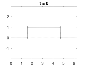
Figure 1: Real (solid) and imaginary (dashed) profiles of the piece-wise constant initial function (27).

Using Octave, we plot the real and imaginary parts of the solution (28) for $n=3$, $4$, $5$ at the rational time $t=\frac{2\pi}{3}$ by truncating the series and taking around 1000 terms. In Figure 2, we consider $\theta=\frac{1}{4}$ and observe piece-wise constant profiles. This confirms the first part of Theorem 2.1 which implies that the revival effect appears for rational values of $\theta\in(0,1)$. On the other hand for irrational values, the second part of Theorem 2.1 implies that the revival effect breaks down at rational times and the solution becomes continuous on $[0,2\pi]$ and such that $e^{i2\pi\theta}u(0,t)=u(2\pi,t)$, which is exactly what we observe in Figure 3. In particular, in Figure 3 we see that the solution profiles have the form of continuous but nowhere differentiable functions, indicating that the fractalisation effect occurs at rational times when $\theta$ is irrational. The latter is true at least for $n=3$, with the fractal dimension being $3/2$, as we deduced in Section 4. In contrast to the higher-order models, the second-order case exhibits revivals at rational times for any choice of $\theta\in(0,1)$. This is illustrated in Figure 4 where we plot the real and imaginary parts of (28), when $n=2$ and $t=\frac{2\pi}{3}$, and we observe piece-wise constant profiles for both $\theta=\frac{1}{4}$ and $\theta=\frac{\sqrt{2}}{4}$, as expected by (25).

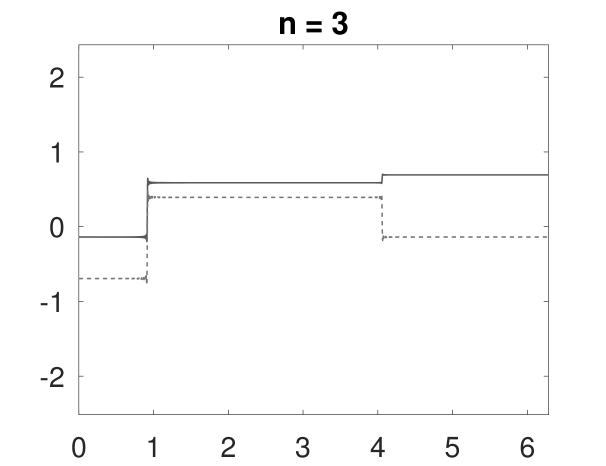
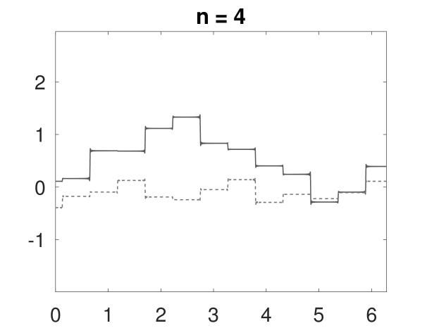
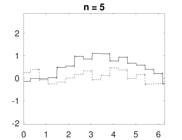
Figure 2: Real (solid) and imaginary (dashed) profiles of the solution (28) at rational time $t=\frac{2\pi}{3}$ when $\theta=\frac{1}{4}$ and $n=3$, $4$, $5$.

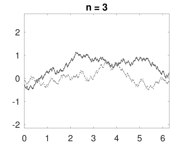
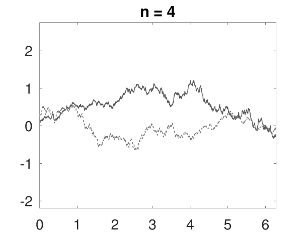
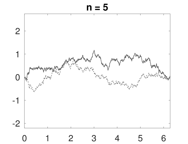
Figure 3: Real (solid) and imaginary (dashed) profiles of the solution (28) at rational time $t=\frac{2\pi}{3}$ when $\theta=\frac{\sqrt{2}}{4}$ and $n=3$, $4$, $5$.

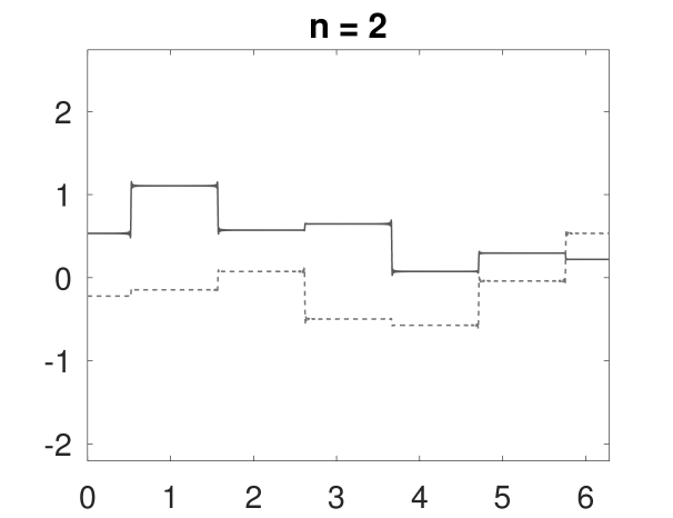
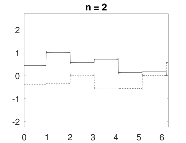
Figure 4: Real (solid) and imaginary (dashed) profiles of the solution (28) at rational time $t=\frac{2\pi}{3}$ when $n=2$ and $\theta=\frac{1}{4}$ or $\theta=\frac{\sqrt{2}}{4}$, respectively.

6 Two non-linear equations

The revival and fractalisation phenomena have also been considered in the non-linear regime. In [12, 23], Erdoğan and Tzirakis examined the Talbot effect under periodic boundary conditions on $[0,2\pi]$ in the context of the cubic non-linear Schrödinger (NLS) equation

$$\partial_{t}u(x,t)=i\partial_{x}^{2}u(x,t)+i|u(x,t)|^{2}u(x,t)$$

and the Korteweg–de Vries (KdV) equation

$$\partial_{t}u(x,t)=-\partial_{x}^{3}u(x,t)-2u(x,t)\partial_{x}u(x,t),$$

respectively. The results in [12] and [23] showed that for initial data of bounded variation, the difference between the solution and the linear evolution, at any positive time, is more regular than the initial function. Thus, in both cases, the revival/fractalisation dichotomy is characterised in terms of change in the regularity of the solution at rational/irrational times. Numerical evidence on the Talbot effect for both equations can be found in the papers of [24] and [25] by Chen and Olver.

Similar to the FLS equation, the cubic NLS equation is invariant under the Galilean transformation

$$u(x,t)=e^{-i\theta^{2}t}e^{i\theta x}\mathcal{T}_{2\theta t}z(x,t).$$

Therefore, we can extend the results in [12] from the periodic to the quasi-periodic setting.

Theorem 6.1.

Fix $\theta\in(0,1)$ and consider the quasi-periodic problem for the NLS equation

$$\partial_{t}u(x,t)=i\partial_{x}^{2}u(x,t)+i|u(x,t)|^{2}u(x,t),\quad u(x,0)=u_{0}(x),$$ (29)

$$e^{i2\pi\theta}u(0,t)=u(2\pi,t),\quad e^{i2\pi\theta}\partial_{x}u(0,t)=\partial_{x}u(2\pi,t).$$

Assume that $u_{0}$ is of bounded variation on $[0,2\pi]$. Then, we have the following.

• For rational values of $t/2\pi$, the solution $u(x,t)$ is a bounded function with at most countably many discontinuities.

• If $t/2\pi$ is an irrational number, then the solution $u(x,t)$ is a continuous function of $x\in[0,2\pi]$ and such that $e^{i2\pi\theta}u(0,t)=u(2\pi,t)$.

Proof.

Due to the Galilean invariance of the cubic NLS equation, the solution to the quasi-periodic problem (29) is given by

$$u(x,t)=e^{-i\theta^{2}t}e^{i\theta x}\mathcal{T}_{2\theta t}z(x,t),$$

where $z(x,t)$ solves the cubic NLS with periodic boundary conditions on $[0,2\pi]$

$$\partial_{t}z(x,t)=i\partial_{x}^{2}z(x,t)+i|z(x,t)|^{2}z(x,t),\quad z(x,0)=z_{0}(x),$$

$$z(0,t)=z(2\pi,t),\quad\partial_{x}z(0,t)=\partial_{x}z(2\pi,t),$$

and with initial value $z_{0}(x)=e^{-i\theta x}u_{0}(x)$. Since $u_{0}$ is a function of bounded variation, the function $z_{0}$ is also of bounded variation as the product of the non-zero continuous function $e^{-i\theta x}$ and $u_{0}$. Moreover, from [12, Theorem 1], we know that the statement of the theorem holds for the solution $z(x,t)$ to the periodic problem. Thus, the theorem holds for $u(x,t)$ as well. ∎

If we further assume that the function $z_{0}(x)=e^{-i\theta x}u_{0}(x)$ does not belong to any of the Sobolev space $H^{s}_{\text{per}}(0,2\pi)$, for any $s>1/2$, then we can deduce that either the real or the imaginary part of the solution $u(x,t)$ to the quasi-periodic problem (29) has fractal dimension $3/2$ at irrational times, since the same is true of the solution to the periodic problem, see [12, Theorem 1].

Compared to the quasi-periodic cubic NLS, the previous trick does not work in the case of the quasi-periodic KdV equation

$$\partial_{t}u(x,t)=-\partial_{x}^{3}u(x,t)-2u(x,t)\partial_{x}u(x,t),\quad u(x,0)=u_{0}(x),$$ (30)

$$e^{i2\pi\theta}\partial_{x}^{m}u(0,t)=\partial_{x}^{m}u(2\pi,t),\quad m=0,1,2,\quad\theta\in(0,1).$$

Therefore, we describe below two possible ideas in order to examine the revival and fractalisation effects in this case.

Under the transformation

$$u(x,t)=e^{i(\theta^{3}t+\theta x)}w(x,t),$$

the quasi-periodic problem (30) is converted to the periodic problem

$$\partial_{t}w(x,t)=\big{(}-\partial_{x}^{3}-3i\theta\partial_{x}^{2}+3\theta^{2}\partial_{x}\big{)}w(x,t)+N(x,t,w,\partial_{x}w),\quad w(x,0)=e^{-i\theta x}u_{0}(x),$$ (31)

$$\partial_{x}^{m}w(0,t)=\partial_{x}^{m}w(2\pi,t),\quad m=0,1,2,$$

where the non-linear term is given by

$$N(x,t,w,\partial_{x}w)=-e^{i(\theta^{3}t-\theta x)}\big{(}2i\theta w^{2}(x,t)+2w(x,t)\partial_{x}w(x,t)\big{)}.$$

First, we remark that, to our knowledge, there is no result that indicates the well-posedness in $L^{2}(0,2\pi)$ of either of the two initial-boundary value problems (30) and (31). Therefore, a first direction would be to analyse this aspect. We suspect that the framework provided by Ruzhanski and Tokmagambeto in [26] should be valuable for the analysis of the quasi-periodic problem (30), whereas for the corresponding periodic problem (31) it might be feasible to adopt some of the arguments of Miyaji and Tsutsumi in [27] on the analysis of the periodic third-order Lugiato-Lefever equation in conjunction with the more recent work on the Talbot effect for the same equation [28] by Cho, Kim and Seo.

Finally, if we assume that there exists a well-posed setting for either (30) or (31), then a natural question that arises is if the revival phenomenon breaks whenever $\theta$ is irrational, similar to the corresponding linear problems. In other words, if we fix $\theta$ to be an irrational number in $(0,1)$, then is there a smoothing effect on the solution of either (30) or (31) at rational times ($t/2\pi\in\mathbb{Q}$)?

7 Conclusion

The main goal of this work was to examine the revival effect in the context of time-evolution problems with quasi-periodic boundary conditions. Theorem 2.1 establishes that for a piece-wise continuous initial condition in $L^{2}(0,2\pi)$, the quasi-periodic problem (1) of order $n\geq 3$ supports the revival effect at rational times only when the boundary parameter $\theta$ is a rational number. Otherwise, for irrational values of $\theta$, the solution at rational times becomes continuous and quasi-periodic, so the revival (of the initial jump discontinuities) breaks down.

The proof of Theorem 2.1 was obtained as a consequence of combining Lemma 3.5 and Theorem 2.2. Lemma 3.5 allows to study the revival effect in the quasi-periodic problem (1) by means of the periodic problem (4). In turn, Theorem 2.2 illustrates that the periodic problem (4) supports the revival property if and only if $\theta$ is rational. The latter also implies that periodic linear dispersive PDEs with polynomial dispersion relation of order $n\geq 3$ can exhibit revivals only when the coefficients of the dispersion relation are all rational.

Further consequences of our approach included the verification and the extension in the quasi-periodic setting and for any $\theta\in(0,1)$ of the Talbot effect in the free linear Schrödinger and the cubic non-linear Schödinger equations, respectively.

Acknowledgements The author thanks Lyonell Boulton and Beatrice Pelloni for their useful comments and suggestions on previous versions of the manuscript. The work was funded by EPSRC through Heriot-Watt University support for Research Associate positions, under the Additional Funding Programme for the Mathematical Sciences. Also, part of this research was conducted during the author’s PhD studies which were supported by the Maxwell Institute Graduate School in Analysis and its Applications, a Centre for Doctoral Training funded by EPSRC (grant EP/L016508/01), the Scottish Funding Council, Heriot-Watt University and the University of Edinburgh.

References

- [1] Peter J Olver “Dispersive quantization” In The American Mathematical Monthly 117.7 Taylor & Francis, 2010, pp. 599–610
- [2] Michael Berry, Irene Marzoli and Wolfgang Schleich “Quantum carpets, carpets of light” In Physics World 14.6 IOP Publishing, 2001, pp. 39–46
- [3] Vasilis Chousionis, M Burak Erdoğan and Nikolaos Tzirakis “Fractal solutions of linear and nonlinear dispersive partial differential equations” In Proceedings of the London Mathematical Society 110.3 Oxford University Press, 2014, pp. 543–564
- [4] M Burak Erdoğan and Nikolaos Tzirakis “Dispersive partial differential equations. Wellposedness and applications” London Mathematical Society Student Texts. Cambridge University Press, Cambridge, 2016
- [5] Lyonell Boulton, George Farmakis and Beatrice Pelloni “Beyond periodic revivals for linear dispersive PDEs” In Proceedings of the Royal Society A 477.2251 The Royal Society Publishing, 2021, pp. 20210241
- [6] Zihan Yin, Jing Kang and Changzheng Qu “Dispersive quantization and fractalization for multi-component dispersive equations” In Physica D: Nonlinear Phenomena 444 Elsevier, 2023, pp. 133598
- [7] George Farmakis et al. “New Revival Phenomena for Bidirectional Dispersive Hyperbolic Equations” In arXiv preprint arXiv:2309. 14890, 2023
- [8] Peter J Olver, Natalie E Sheils and David A Smith “Revivals and Fractalisation in the linear free space Schrödinger equation” In Quarterly of Applied Mathematics 78.2, 2020, pp. 161–192
- [9] Lyonell Boulton, Peter J Olver, Beatrice Pelloni and David A Smith “New revival phenomena for linear integro–differential equations” In Studies in Applied Mathematics 147.4 Wiley Online Library, 2021, pp. 1209–1239
- [10] David A Smith “Revivals and Fractalization” In Dynamical System Web, 2020, pp. 1–8
- [11] Georgios Farmakis “Revivals in Time Evolution Problems”, 2022
- [12] M. B. Erdoǧan and N. Tzirakis “Talbot effect for the cubic non-linear Schrödinger equation on the torus” In Mathematical Research Letters 20.6 International Press of Boston, Inc., 2013, pp. 1081–1090
- [13] David Borthwick “Spectral Theory: Basic Concepts and Applications” Springer Nature, 2020
- [14] John M Ball “Strongly continuous semigroups, weak solutions, and the variation of constants formula” In Proceedings of the American Mathematical Society 63.2, 1977, pp. 370–373
- [15] Felipe Linares and Gustavo Ponce “Introduction to nonlinear dispersive equations” Second edition. Universitext. Springer, New York, 2015
- [16] Gregory J Gbur “Mathematical methods for optical physics and engineering” Cambridge University Press, Cambridge, 2011
- [17] Michael Victor Berry and Sz Klein “Integer, fractional and fractal Talbot effects” In Journal of Modern Optics 43.10 Taylor & Francis, 1996, pp. 2139–2164
- [18] KI Oskolkov “A class of I.M. Vinogradov’s series and its applications in harmonic analysis” In Progress in approximation theory 19 Springer Series in Computational Mathematics, Springer, New York, 1992, pp. 353–402
- [19] Michael Taylor “The Schrödinger equation on spheres” In Pacific Journal of Mathematics 209.1 Mathematical Sciences Publishers, 2003, pp. 145–155
- [20] Pertti Mattila “Geometry of sets and measures in Euclidean spaces. Fractals and rectifiability” Cambridge Studies in Advanced Mathematics. Cambridge University Press, Cambridge, 1999
- [21] Igor Rodnianski “Fractal solutions of the Schrödinger equation” In Contemporary Mathematics 255 Providence, RI; American Mathematical Society; 1999, 2000, pp. 181–188
- [22] Lev Kapitanski and Igor Rodnianski “Does a quantum particle know the time?” In Emerging applications of number theory The IMA Volumes in Mathematicsits Applications, 109, Springer, New York, 1999, pp. 355–371
- [23] Mehmet Burak Erdoğan and Nikolaos Tzirakis “Global smoothing for the periodic KdV evolution” In International Mathematics Research Notices 2013.20 OUP, 2013, pp. 4589–4614
- [24] Gong Chen and Peter J Olver “Dispersion of discontinuous periodic waves” In Proceedings of the Royal Society A 469.2149 The Royal Society Publishing, 2013, pp. 20120407
- [25] Gong Chen and Peter J Olver “Numerical simulation of nonlinear dispersive quantization” In Discrete and Continuous Dynamical Systems 34.3 American Institute of Mathematical Sciences, 2014, pp. 991–1008
- [26] Michael Ruzhansky and Niyaz Tokmagambetov “Nonharmonic analysis of boundary value problems” In International Mathematics Research Notices 2016.12 Oxford University Press, 2016, pp. 3548–3615
- [27] Tomoyuki Miyaji and Yoshio Tsutsumi “Existence of global solutions and global attractor for the third order Lugiato–Lefever equation on T” In Annales de l’Institut Henri Poincaré C, Analyse non linéaire 34.7, 2017, pp. 1707–1725
- [28] Gunwoo Cho, Seongyeon Kim and Ihyeok Seo “Talbot effect for the third order Lugiato-Lefever equation” In arXiv preprint arXiv:2304.10964, 2023