Spontaneous baryogenesis and generation of gravitational waves in a new model of quintessential $\alpha$-attractor

Abstract

We apply a new version of quintessential $\alpha$-attractor inflaton potential (arXiv: 2305.00230 [gr-qc]) to make a detailed analysis of the phenomenon of spontaneous baryogenesis in the post-inflationary kination period. In this context, we compute various temperatures viz., the temperature at the end of inflation (or start of kination) ($T_{\mathrm{end}}$), maximum thermalization temperature ($T_{\mathrm{th}}$), freeze-out temperature ($T_{F}$), the temperature of radiation domination ($T_{\mathrm{rad}}$), their respective number of e-folds, the densities viz., total field energy density ($\rho_{\mathrm{kin}}$), radiation density ($\rho_{\mathrm{rad}}$) and the freeze-out values of baryon-to-entropy ratio ($\eta_{F}$) at different mass scales ($M$, $\tilde{M}$), as functions of $\alpha$. The numerical calculations show that the baryon-to-entropy ratio is obtained as: for $\alpha=0.29-0.30$, $\eta_{F}=8.7\times 10^{-11}-8.5\times 10^{-11}$ and for $\alpha=4.2-4.3$, $\eta_{F}=8.5\times 10^{-11}-8.6\times 10^{-11}$. The results are found to satisfy experimental bounds quite satisfactorily. We also find a blue-tilted spectrum of relic gravitational waves (GW) of frequencies lying in two narrow bands corresponding to the two regions of $\alpha$, indicated above, viz., $f_{\mathrm{end}}=2.00\times 10^{10}-2.10\times 10^{10}$ Hz for lower region of $\alpha$ and $f_{\mathrm{end}}=2.12\times 10^{10}-2.11\times 10^{10}$ Hz for higher region of $\alpha$, during transition from inflation to kination, which is supported by current literature. The present-day peak values of the amplitudes of GWs emitted during radiation domination, ($(\Omega_{\mathrm{GW},0}^{(\mathrm{RD})})_{\mathrm{peak}}$), are found to be $\sim 10^{-7}$, which is consistent with the requirement for nucleosynthesis and the associated root-mean-square values, ($\Omega_{\mathrm{GW},0}^{(\mathrm{RD})}\sim 10^{-18}$), conform to the characteristic strain of the ongoing GW-detectors. In this way, a unified picture of the roles of quintessential $\alpha$-attractor model, considered here, in inflation, quintessence, spontaneous baryogenesis and the gravitational waves production, emerges from the present study.

I Introduction

The matter-antimatter asymmetry is an intriguing phenomenon in the frontiers of particle physics and cosmology. There is no known exact mechanism to generate the tiny baryon-to-entropy ratio $\eta\approx(8.6\pm 0.1)\times 10^{-11}$ [1, 2, 3, 4], which is a crucial requirement for big bang nucleosynthesis (BBN) and is almost fixed from the early universe to the present day. One can imagine that, due to some exotic process in the early universe, baryon number conservation was violated, which led to the excess number densities of particles over those of anti-particles. This process is popularly known as Baryogenesis. In 1967, Andrei Sakharov proposed three criteria [5], based on symmetry principles, in order to achieve the baryon asymmetry: i) Baryon number ($B$) violation, ii) Charge conjugation ($C$) and charge conjugation-parity ($CP$) violations and iii) thermal non-equilibrium in presence of charge conjugation-parity-time reversal ($CPT$) invariance. The first condition is trivial in order to achieve a baryon asymmetric universe with $\Delta B\neq 0$. Since any stipulation of $C$ and $CP$ invariance would be compatible with the $B$ invariance, $C$ and $CP$ violations are essentially needed to ensure $B$ violation [6]. This is Sakharov’s second criterion. Now, to maintain the excess of baryons the rate of $B$ violation should be very small compared to the expansion rate of the universe, otherwise the $CPT$ invariance and hence the $T$ violation would bring back the universe in a state of $\Delta B=0$, through thermal equilibrium. It is only possible by the ‘departure from thermal equilibrium’, which is Sakharov’s third condition. The last condition is important because in a phase of matter-antimatter symmetry, no preferred direction of time can be made, but thermal out-of equilibrium sets a unique direction of flow of time from the early universe to the present day.

The Standard Model (SM) of particle physics can accommodate large $B$ violation [7] at high temperature by sphaleron transition [8] between the degenerate $SU(2)$ vacua and very small CP violation [6]. However, it can not meet Sakharov’s third criterion, as this requires a Strong First Order Electroweak Phase Transition (SFOEWPT) [9, 10, 11, 12], which is not possible to achieve in SM [13, 14, 15] for experimentally favored Higgs mass [16, 17].

This was already evident in the large value ($\sim 10^{12}$) [7] of the ratio ($B$ violation rate/universe expansion rate), calculated in the SM. However, a small value of the ratio consistent with the SFOEWPT can be obtained in a number of Beyond Standard Models (BSMs) (for a review, see Ref. [9]), at the TeV scale.

Another angle of comparison between the SM and the BSMs is the fact that in the former the Higgs mass is unstable against the bosonic and the fermionic loop corrections, whereas in the latter it is not, due to the cancellation effects. These theoretical findings make the situation somewhat confusing because the experimental Higgs (mass $\sim 126$ GeV) in the LHC experiments [18, 19] is SM-like. Only future collider experiments might resolve some of these issues by either proving or disproving the BSMs.

An interesting alternative approach is to relax Sakharov’s third criterion by invoking an effective formulation beyond conventional particle physics models in order to generate the required baryon asymmetry in a scenario of thermal equilibrium à la spontaneous baryogenesis (SB) [20, 21, 22, 23, 24, 25, 26, 27, 28, 29, 30, 31, 32, 4, 33, 34, 35, 36, 37, 38, 39, 40, 41]. This approach is highly non-trivial because, generically, the average value of baryon number density in thermal equilibrium is zero. However, a non-zero value can be obtained even in thermal equilibrium, by the spontaneous breaking of the CPT invariance [20] due to the kinetic energy of a rolling scalar field $\phi$. This is particularly seen to manifest through the derivative coupling of the scalar field with a non-conserving baryon current $J^{\mu}_{b}$ as $\partial_{\mu}\phi J^{\mu}_{b}$ [4, 29]. The $\phi$ field acts as a pseudo-Nambu-Goldstone boson [42, 43] in an approximate $U(1)$ symmetry [20, 44, 43]. (See for related studies in particle physics, [22, 45] and in inflationary cosmology, [44, 43, 46].)

Nowadays, in the interface of particle physics and cosmology, this scenario is popularly known as quintessential baryogenesis [47, 48, 49, 50, 51, 52] in the paradigm of inflationary quintessence [53], since the idea of rolling scalar field is inbuilt in this kind of inflationary framework. Quite interestingly, here, the scalar field playing the roles of inflaton and quintessence, can also trigger the process of baryogenesis. The quintessential inflaton field when traverses through the kination regime [54] after inflation, particle production starts to reheat the universe either gravitationally [55, 56, 57, 58, 59, 60] or through instant preheating (IP) [61, 62, 63]. These particles interact with the scalar field leading to SB at a temperature between $\sim 10^{8}-10^{12}$ GeV, which is higher than that of radiation era ($\sim 10^{7}$ GeV). In this course, the $\phi$-field spends longer time in the kination period than in inflation. Consequently, thermal equilibrium manifests before radiation fills the universe. The rate of baryon non-conserving process decreases, as the universe cools down due to Hubble expansion, which ceases to act below a certain temperature $T_{F}$, called the freeze-out temperature. The temperature at which baryogenesis takes place, should be above $T_{F}$ otherwise the CPT symmetry could be restored and baryon asymmetry would not occur. The actual value of $T_{F}$ and the energy scale of baryon non-conservation depend on the specific physical processes involved, provided that the back reactions of the reheating particles on the scalar field dynamics are negligibly small [64], ensuring that the field velocity $\partial_{0}\phi$ does not vanish.

The most clear evidence of quintessential SB scenario in the present and future experiments would be the detection of the relic gravitational waves, originated from the quantum fluctuations during inflation at sub-Hubble scale, which re-enter the Hubble horizon at different epochs. During transition from inflation to kination, due to a sharp change in the metric structure [47], gravitational waves (GWs) of high frequencies $\sim 10^{10}$ Hz, called blue-tilted GWs are emitted, while during matter domination red-tilted GWs of frequencies $\sim 10^{-17}-10^{-19}$ Hz are emitted [65, 50]. The stochastic signature of the former type of GWs are instrumental in the verification of various BBN constraints [66, 67]. Overproduction of GWs would lead to spike in their energy densities [68], which could be threatening to nucleosynthesis process. These aspects specifically depend upon the particular modes of particle production involved after inflation. Specifically, gravitational reheating produces GW-energy too large to begin the nucleosynthesis, therefore inefficient to satisfy the required BBN constraints [66, 67], whereas the IP is more efficacious in this regard. Another important aspect is the amplitudes of the GWs, called the characteristic strain, which is extremely small $\sim 10^{-18}$ (see figure 11), thereby making the detection processes too difficult and complicated. In fact such a tiny value of the GW-amplitude carries indirect signatures of small values of tensor-to-scalar ratio and the amplitudes of CMB $B$ modes. That is why, the detection of primordial GWs are the targets of many ongoing and forthcoming cosmological surveys. See section IV.4 for details.

According to the current studies, the quintessential versions of $\alpha$-attractors have been identified to be efficacious in explaining the observational bounds of both inflation and dark energy. See Ref. [69] for example. Recently in Ref. [70], the present authors have explored various aspects of the quintessential inflationary regime for a specific model, by constraining the parameter $\alpha$ and fixing the energy scales of inflation and quintessence. They showed that for $0.1\leq\alpha\leq 4.3$, the model is just appropriate for satisfying the Planck data with $68\%$ CL. Now, it will be interesting to examine this new model in the context of SB. The present paper, therefore, aims at revisiting the scenario of SB with the newly obtained range of $\alpha$ and study the applicability of the new potential [70] in estimating various constraints of quintessential inflationary baryogenesis and the associated gravitational waves.

The outline of the present paper is as follows. It contains a preamble in Section II, explaining the kination period through the definition of a number of temperatures in the context of post-inflationary particle production. Section III gives a brief review of SB. The new quintessential $\alpha$-attractor inflaton potential is applied to analyze the baryogenesis scenario, whose results are illustrated in Section IV. The spectra of relic gravitational waves associated with this potential are also analyzed in the same section (sub-section IV.4). Finally, Section V contains some concluding remarks.

II The post-inflationary kination period

In the standard formulation of inflationary quintessence [53], the $\phi$ field enters into a kinetic energy dominated phase called kination [54], just after the end of inflation. This period of expansion can be characterized by the scale factor ($a$)-dependent energy density [68]

$$\rho_{\mathrm{kin}}(a)=\rho_{\mathrm{end}}\left(\frac{a_{\mathrm{end}}}{a}\right)^{6}$$ (1)

and Hubble rate

$$H_{\mathrm{kin}}(a)=\sqrt{\frac{\rho_{\mathrm{kin}}(a)}{3M_{p}^{2}}}=H_{\mathrm{end}}\left(\frac{a_{\mathrm{end}}}{a}\right)^{3}.$$ (2)

Here, the subscript ‘end’ denotes the respective parameters at the point where the inflation ends (and kination begins) and $M_{p}(=1/\sqrt{8\pi G})$ is the reduced Planck mass. The constants $\rho_{\mathrm{end}}$ and $H_{\mathrm{end}}$ are the inputs from a specific model of inflation, depending on the nature of the potential $V(\phi)$. At the end of inflation, $\phi$ reaches $\phi_{\mathrm{end}}$ and the corresponding value of the potential, $V_{\mathrm{end}}=V(\phi_{\mathrm{end}})$, is obtained from equating the first potential slow-roll parameter $\epsilon_{V}$ to unity. Since in this period of expansion, the kinetic energy of the $\phi$ field grows up to be comparable with the potential energy (i.e. $\dot{\phi}^{2}\sim V(\phi)$), we can write

$$\rho_{\mathrm{kin}}=\frac{\dot{\phi}^{2}}{2}+V(\phi)\approx\frac{3}{2}\dot{\phi}^{2}.$$ (3)

The end-value of the potential is therefore induced in $\rho_{\mathrm{end}}$ and $H_{\mathrm{end}}$ through the approximation, $\dot{\phi}_{\mathrm{end}}^{2}\approx V_{\mathrm{end}}$ as

$$H_{\mathrm{end}}=\sqrt{\frac{\rho_{\mathrm{end}}}{3M_{p}^{2}}}\approx\sqrt{\frac{V_{\mathrm{end}}}{2M_{p}^{2}}}.$$ (4)

Now from Eqs. (1), (3) and (4) we get

$$\frac{3}{2}\dot{\phi}^{2}\approx\frac{3}{2}V_{\mathrm{end}}\left(\frac{a_{\mathrm{end}}}{a}\right)^{6},$$ (5)

which yields the field velocity of the form

$$\dot{\phi}\approx\sqrt{V_{\mathrm{end}}}\left(\frac{a_{\mathrm{end}}}{a}\right)^{3}.$$ (6)

Here the constants $\sqrt{V_{\mathrm{end}}}$ and $a_{\mathrm{end}}$ indicate that the field dynamics depends on the particular inflationary model. However, Ref. [68] shows that if the kinetic energy of the field is taken to be extremely large ($\dot{\phi}^{2}\gg V(\phi)$) in comparison to the potential energy (i.e. complete free-fall), then the dynamics of the field will be model-independent. On the other hand, in our formalism, we have considered kinetic energy to be comparable to the potential energy during kination, and therefore we have always retained the effects of $V(\phi)$ during kination in the constants like $V_{\mathrm{end}}$ and $a_{\mathrm{end}}$ following Ref. [53], as it will be shown, the potential will have a significant role to play in the process of SB.

Now, due to the expansion of the universe, $\dot{\phi}$ becomes significantly small during kination with the increase in the scale factor $a$ and thereby the total energy density diminishes rapidly until radiation takes over through reheating associated with particle production. During the transition from inflation to kination, due to a non-adiabatic change of the metric structure [47], an easy-to-realize mechanism of reheating is gravitational particle production (GPP) [55, 56, 57, 58, 59, 60]. But it is not so effective so far as various constraints of BBN [63, 50] are concerned. For example, GPP produces an insufficient amount of radiation density to start nucleosynthesis. GPP has been therefore replaced by an efficient method, called instant preheating (IP) [61, 62, 63]. See Ref. [63] for details of this procedure, specifically for $\alpha$-attractor. Generally, it is an instantaneous (within one cycle of oscillation of the inflaton field), non-perturbative mechanism of reheating due to the effects of ‘broad parametric resonance’ (BPR) [71, 72, 73, 61], characterized by fast energy transfer from the inflaton field to the superheavy massive particles produced, whose masses are typically $\sim 10^{17}-10^{18}$ GeV [61]. But in the case of quintessential inflation, as there is no minimum where the inflaton field can oscillate, rather a quintessential run-away, the BPR does not work. Just after the end of inflation, almost instantaneously the non-oscillating inflaton field produces superheavy particles, which again decay into fermions or bosons depending upon the nature of interactions. The elementary particles thus created give rise to a radiation density [74, 63, 50, 68]

$$\rho_{\mathrm{rad}}(a)=\left[\frac{gM_{p}H_{\mathrm{end}}}{2\pi^{3/2}}\left(\frac{a_{\mathrm{end}}}{a}\right)^{2}\right]^{2},$$ (7)

where $g(<1)$ is the positive coupling of IP. The associated temperature [75, 68] in unit of $M_{p}$ can be derived from Eq. (7) as,

$$\begin{split}T(a)&=\left(\frac{30}{\pi^{2}g_{*}}\rho_{\mathrm{rad}}(a)\right)^{1/4}\\ &=\left(\frac{15g^{2}M_{p}^{2}H_{\mathrm{end}}^{2}}{2\pi^{5}g_{*}}\right)^{1/4}\left(\frac{a_{\mathrm{end}}}{a}\right).\end{split}$$ (8)

Here, $g_{*}$ denotes the total number of degrees of freedom of the relativistic particles produced through IP. The factor in the first bracket containing constant terms has the dimension of temperature. Therefore it can be taken as a constant temperature term,

$$T_{\mathrm{end}}=\left(\frac{15g^{2}M_{p}^{2}H_{\mathrm{end}}^{2}}{2\pi^{5}g_{*}}\right)^{1/4},$$ (9)

such that,

$$T=T_{\mathrm{end}}\left(\frac{a_{\mathrm{e}nd}}{a}\right).$$ (10)

$T_{\mathrm{end}}$ actually denotes the temperature at the instant of ending of inflation and beginning of kination at the scale factor $a=a_{\mathrm{end}}$. It is model-dependent, since, according to Eqs. (4) and (9) $T_{\mathrm{end}}\propto V_{\mathrm{end}}^{1/4}$.

Now, with the expansion of the universe, the decay rate with coupling $\beta$ [74, 76, 50] of the massive particles produced through IP decreases and let at $a=a_{\mathrm{th}}$ it becomes equal to the Hubble rate of expansion (see Eq. (2)). At this particular scale factor, thermal equilibrium commences and it is found to be,

$$a_{\mathrm{th}}=\left(\frac{2^{9/2}\pi^{6}T_{\mathrm{end}}^{4}}{g^{3}\beta^{4}M_{p}^{3}H_{\mathrm{end}}}\right)^{1/4}a_{\mathrm{end}},$$ (11)

which is, when applied in Eq. (10), gives the temperature at the thermal equilibrium,

$$T_{\mathrm{th}}=\left(\frac{g^{3}\beta^{4}M_{p}^{3}H_{\mathrm{end}}}{2^{9/2}\pi^{6}}\right)^{1/4}.$$ (12)

This is the maximum temperature of the universe after inflation that can be attained in thermal equilibrium, called the maximum thermalization temperature [47]. After this event, the total energy density of the scalar field becomes weaker and, as a consequence, radiation starts to emerge as a major component of the universe.

Eq. (10) can be instrumental in evaluating the temperature during the era of radiation domination. Let us call the temperature as $T_{\mathrm{rad}}$ when the radiation domination starts and the corresponding scale factor as $a_{\mathrm{rad}}$. At this scale factor, there will be a cross-over between two densities $\rho_{\mathrm{kin}}$ and $\rho_{\mathrm{rad}}$ (see Eqs. (1) and (7)), which means that at this stage $\rho_{\mathrm{kin}}(a_{\mathrm{rad}})=\rho_{\mathrm{rad}}(a_{\mathrm{rad}})$ (this happens at a particular value of e-folds) and thereafter $\rho_{\mathrm{rad}}$ will exceed $\rho_{\mathrm{kin}}$. This aspect will be illustrated in the specific case of $\alpha$-attractor potential in Section IV. Now, from Eqs. (1) and (7) we get

$$a_{\mathrm{rad}}=\left(\frac{12\pi^{3}}{g^{2}}\right)^{1/2}a_{\mathrm{end}}$$ (13)

and from Eqs. (10) and (13) we have

$$T_{\mathrm{rad}}=\left(\frac{g^{2}}{12\pi^{3}}\right)^{1/2}T_{\mathrm{end}}.$$ (14)

Eq. (13) (Eq. (14)) shows that the ratio of the scale factors (temperatures) in the radiation domination era and the corresponding end-value depends only on the coupling constant of IP. In Section IV, this finding will play an important role in analyzing the evolution of the universe during kination, for the potential considered in the present paper.

The three temperatures $T_{\mathrm{end}}$, $T_{\mathrm{th}}$ and $T_{\mathrm{rad}}$ are crucial in jointly framing the whole scenario of the kination period. We can determine their values by doing a model-independent estimate. We take the help of an empirical formula [77] relating the inflationary energy scale (in the unit of reduced Planck mass) with the tensor-to-scalar ratio $r$:

$$V^{1/4}(r)\approx r^{1/4}\times\left(\frac{10^{16.5}}{2.43\times 10^{18}}\right)M_{p}.$$ (15)

A good slow-roll inflaton potential always supports a small value of $r$ ($r<0.064$ [78, 79]) and hence a small $\epsilon_{V}$, since $r=16\epsilon_{V}$. Therefore, it will be reasonable to consider a rough estimation $V\approx V_{\mathrm{end}}$, in a model-independent way. Thus, if we take $r=0.05$, then from Eqs. (15) and (4), we obtain

$$V_{\mathrm{end}}^{1/4}=6.15\times 10^{-3}M_{p}$$ (16)

and

$$H_{\mathrm{end}}=2.67\times 10^{-5}M_{p}.$$ (17)

Choosing $\beta\sim 10^{-1}$, $g\sim 10^{-4}$ and $g_{*}\sim 10^{2}$ (based on various literature of IP, for example, [61, 63]), we finally obtain

$$T_{\mathrm{end}}=6.46\times 10^{-6}M_{p}=1.57\times 10^{13}\quad\mathrm{GeV},$$ (18)

$$T_{\mathrm{th}}=5.92\times 10^{-7}M_{p}=1.44\times 10^{12}\quad\mathrm{GeV}$$ (19)

and

$$T_{\mathrm{rad}}=3.35\times 10^{-11}M_{p}=8.14\times 10^{7}\quad\mathrm{GeV}.$$ (20)

Eqs. (18) - (20) show that $T_{\mathrm{end}}/T_{\mathrm{th}}\approx 10.9$ and $T_{\mathrm{rad}}/T_{\mathrm{th}}\approx 5.6\times 10^{-5}$. Therefore it is clear that thermal equilibrium is reached shortly after the end of inflation and long before the advent of the radiation era, which is an essential requirement for the SB.

III Basic framework of spontaneous baryogenesis

The relevant Lagrangian here is,

$$\mathcal{L}_{\phi}=\left(-\frac{1}{2}g^{\mu\nu}\partial_{\mu}\phi\partial_{\nu}\phi-V(\phi)-\mathcal{L}_{\mathrm{eff}}\right),$$ (21)

where the quintessential inflaton field $\phi$ is in the Friedmann metric background $g_{\mu\nu}$ of signature $(-,+,+,+)$. In addition, $\phi$ is coupled with a non-conserving baryon current $J^{\mu}$ by the following $CP$-odd effective interaction [47, 4, 50, 52]

$$\mathcal{L}_{\mathrm{eff}}=\frac{\lambda^{\prime}}{M}\partial_{\mu}\phi J^{\mu},$$ (22)

$\lambda^{\prime}$ being a dimensionless coupling constant and the mass scale $M<M_{P}$ signifies a sub-Planckian cut-off of the effective theory. The associated energy-momentum tensor can be obtained from the equation

$$T^{\mu}_{\nu}=\delta^{\mu}_{\nu}\mathcal{L}_{\phi}-2g^{\mu\alpha}\frac{\partial\mathcal{L}_{\phi}}{\partial g^{\alpha\nu}}.$$ (23)

The scalar field $\phi$ is spatially homogenized by the cosmic expansion after inflation. All primordial quantum fluctuations ($\delta\phi$) buried in $\phi$ within the Hubble sphere are transferred to density perturbations, whose imprints are detected in the anisotropies of the cosmic microwave background. The remaining $\phi$ field is now completely classical and time-dependent only. Therefore, in Eq. (23) only $\mu=0$ component of $J^{\mu}$ viz., $J^{0}=n-\bar{n}$ will contribute, which measures the difference between the number densities of baryons ($n$) and ant-baryons ($\bar{n}$). Following these arguments from Eq. (23), the field density takes the form (see Appendix A)

$$\begin{split}\rho&=-T_{0}^{0}=\left(\frac{\dot{\phi}^{2}}{2}+V(\phi)\right)+\left(-\frac{\lambda^{\prime}}{M}\dot{\phi}\left(n-\bar{n}\right)\right)\\ &=\rho_{0}+\left(n\delta\mathcal{E}+\bar{n}\delta\bar{\mathcal{E}}\right),\end{split}$$ (24)

where $\delta\mathcal{E}=-\delta\bar{\mathcal{E}}=-\frac{\lambda^{\prime}\dot{\phi}}{M}$. $\rho_{0}$ is the interaction-free part of the density $\rho$. The second term indicates that, if the field velocity $\dot{\phi}$ is appreciably non-zero (i.e. $\phi$ is a fast-rolling scalar field), then for each baryon (anti-baryon), an extra amount of energy density $\delta\mathcal{E}(\delta\bar{\mathcal{E}})$ would appear in the total energy density budget of the universe. The extra positive and negative energy density terms originate from the interaction term $\partial_{\mu}\phi J^{\mu}$ responsible for spontaneous $CPT$ symmetry breaking at a scale below the Planck mass, as explained in Section I, which ultimately ensure the baryon-excess ($n>\bar{n}$) in the universe. If, on the other hand, $CPT$ symmetry is not broken in thermal equilibrium, there would be no baryon asymmetry i.e. $n=\bar{n}$. We shall calculate $n-\bar{n}$ in the next paragraph and show that it is positive definite. At the thermal equilibrium, this additional energy per baryon (anti-baryon) is recognized as an effective chemical potential $\mu$ ($-\mu$) [4]. Alternative realizations of chemical potentials, in this context, can be seen in Refs. [34, 35].

We explicitly compute the baryon excess by considering the statistical phase space distribution function in thermal equilibrium,

$$f(\epsilon,\mu)=\frac{1}{e^{\left(\frac{\epsilon-\mu}{T}\right)}+1}=\frac{1}{e^{\left(\frac{|\vec{p}|-\mu}{T}\right)}+1},$$ (25)

of an ensemble of massless relativistic baryons of momentum $\vec{p}$ at a particular energy level $\epsilon=|\vec{p}|$ with degeneracy $\tilde{g}$ as,

$$\Delta n=n-\bar{n}=\int\tilde{g}\frac{d^{3}\vec{p}}{(2\pi)^{3}}\left[f(\epsilon,\mu)-f(\epsilon,-\mu)\right],$$ (26)

with the convention $c=\hbar=k_{B}=1$. Under the high temperature approximation, $\mu/T\ll 1$, Eq. (26) reduces to (see Appendix B)

$$\Delta n\approx\frac{\tilde{g}\mu T^{2}}{6}=\frac{\tilde{g}\lambda^{\prime}\dot{\phi}T^{2}}{6M}>0.$$ (27)

The temporal behavior of $\phi$, determined by $\dot{\phi}$, is encoded in the solution of its equation of motion under the effective interaction of Eq. (22) during kination in expanding background. We derive that equation of motion, using Eq. (21) from the Euler-Lagrange equation

$$\left[\partial_{\mu}\left(\frac{\partial}{\partial_{\mu}\phi}\right)-\frac{\partial}{\partial\phi}\right]\sqrt{-g}\mathcal{L}_{\phi}=0,$$ (28)

as (see Appendix C)

$$\left[1-\frac{\tilde{g}}{6}\left(\frac{\lambda^{\prime}M_{p}}{M}\right)^{2}\left(\frac{T}{M_{p}}\right)^{2}\right]\left(\ddot{\phi}+3H\dot{\phi}\right)+\frac{dV(\phi)}{d\phi}=0.$$ (29)

The second term in the third bracket signifies the back-reaction on $\phi$ of the coupling described in Eq (22). According to the Carroll bound [64, 10] $\frac{\lambda^{\prime}M_{p}}{M}<8$, and as described in Section I, the baryon asymmetry operates at temperature $T$ lying in the range $T_{F}<T<T_{\mathrm{th}}$, where $T_{\mathrm{th}}\sim 10^{-7}M_{p}$ (see Eq. (19)), which implies $T/M_{p}\ll 1$. Therefore the effect of back-reaction vis-à-vis the second term is very small. Then from Eq. (29) the dynamical equation of $\phi$ reduces to

$$\ddot{\phi}+3H\dot{\phi}+\frac{dV(\phi)}{d\phi}\approx 0,$$ (30)

which is the well-known Klein-Gordon equation of the scalar field $\phi$.

Now, in the kination regime, the field $\phi$ is predominantly controlled by its kinetic energy density, which is approximately equal (i.e. comparable) to the potential energy density $V(\phi)$ (see Eq. (3)). Therefore, $\frac{dV(\phi)}{d\phi}\approx\frac{d\dot{\phi}^{2}}{d\phi}=0$ (since $\phi$ and $\dot{\phi}$ are mutually independent quantities) and consequently, the potential gradient in Eq. (30) can be neglected. Thus we get

$$\ddot{\phi}+3H\dot{\phi}\approx 0.$$ (31)

Considering $H=\frac{\dot{a}}{a}$ in Eq. (31) we obtain,

$$\frac{1}{a^{3}}\frac{d}{dt}\left(a^{3}\dot{\phi}\right)=0,$$ (32)

whose solution is given by

$$\dot{\phi}=\frac{C}{a^{3}},$$ (33)

where $C$ is a constant. Using the approximation $\dot{\phi}_{\mathrm{end}}=\dot{\phi}(a_{\mathrm{end}})\approx\sqrt{V_{\mathrm{end}}}$ indicated in Section II as initial condition, we obtain $C=\sqrt{V_{\mathrm{end}}}\left(a_{\mathrm{end}}\right)^{3}$ and thus Eq. (33) matches with Eq. (6). Therefore, under negligible amount of back-reaction, the effective interaction gives the same equation of kination, as described in Section II. This indicates that the approximations mentioned in Section II are fairly consistent with the framework of SB.

According to Eqs. (6) and (10) the field velocity $\dot{\phi}$ can be parameterized as a function of temperature as

$$\dot{\phi}(T)=\sqrt{V_{\mathrm{end}}}\left(\frac{T}{T_{\mathrm{end}}}\right)^{3}.$$ (34)

Eqs. (27) and (34) show that the baryon excess $\Delta n$ is only temperature dependent. It is conveniently measured with respect to the entropy density $s$ (given in Refs. [4, 50, 52]) as

$$\begin{split}\eta_{T}&=\left(\frac{\Delta n}{s}\right)=\frac{\left(\frac{\tilde{g}\lambda^{\prime}\dot{\phi}T^{2}}{6M}\right)}{\left(\frac{2\pi^{2}g_{*}T^{3}}{45}\right)}\\ &=\frac{15}{4\pi^{2}}\left(\frac{\lambda^{\prime}}{M}\right)\left(\frac{\tilde{g}}{g_{*}}\right)\left(\frac{\dot{\phi}(T)}{T}\right).\end{split}$$ (35)

This is called the baryon-to-entropy ratio (BTER) at a finite temperature $T$. Since $\dot{\phi}(T)\propto T^{3}$, $\eta_{T}\propto T^{2}$, i.e. $\eta_{T}$ decreases as the temperature of the universe decreases with expansion. But, as explained in Section I, this will continue up to the freeze-out temperature $T_{F}$. Below $T_{F}$ the baryon non-conserving processes fall out of thermal equilibrium and no further baryons are generated. As a result, $\eta_{F}$ saturates at a freeze out value

$$\eta_{F}=\frac{15}{4\pi^{2}}\left(\frac{\lambda^{\prime}}{M}\right)\left(\frac{\tilde{g}}{g_{*}}\right)\left(\frac{\dot{\phi}(T_{F})}{T_{F}}\right),$$ (36)

which acts as a standard measure of the observed baryon asymmetry in the present universe. Therefore it should conform with the experimental value of $\eta$, mentioned in Section I.

Following Eqs. (4), (9), (10), (12) and (34) the freeze out value of the field velocity takes the form

$$\begin{split}\dot{\phi}(T_{F})&=\sqrt{2M_{p}^{2}}H_{\mathrm{end}}\left(\frac{T_{F}}{T_{\mathrm{end}}}\right)^{3}\\ &=\sqrt{2M_{p}^{2}}\beta^{2}\left(\frac{\pi g_{*}}{60}\right)^{3/4}\frac{T_{F}^{3}}{T_{\mathrm{th}}^{2}}.\end{split}$$ (37)

We now finally obtain from Eqs. (36) and (37),

$$\begin{split}\eta_{F}&=\frac{15\sqrt{2}}{4\pi^{2}}\left(\frac{\pi g_{*}}{60}\right)^{3/4}\left(\frac{\tilde{g}}{g_{*}}\right)\left(\frac{\lambda^{\prime}M_{p}}{M}\right)\left(\frac{\beta T_{F}}{T_{\mathrm{th}}}\right)^{2}\\ &=1.8599\times 10^{-4}\times\left(\frac{\lambda^{\prime}M_{p}}{M}\right)\left(\frac{T_{F}}{T_{\mathrm{th}}}\right)^{2},\end{split}$$ (38)

where $\tilde{g}\sim 1$ and we put the values of $g_{*}$ and $\beta$, used for evaluating the temperatures of Eqs. (18) - (20). Here, $T_{\mathrm{th}}$ bears the signature of the inflaton potential, while $M$ and $T_{F}$ are specific to the particular baryon non-conserving process involved. Thus, in precise evaluation of $\eta_{F}$ in light of the observed value, the data for both the inflation and the baryon asymmetry phenomenology play the determining roles. However, in order to keep the thermal equilibrium during baryogenesis, the $T_{F}$ should lie within $T_{\mathrm{rad}}$ and $T_{\mathrm{th}}$. In fact, by the Carroll bound, a rough estimate of $T_{F}$ can be computed as $T_{F}=1.42\times 10^{-10}M_{p}=3.46\times 10^{8}$ GeV, if $T_{\mathrm{th}}$ and $\eta_{F}$ are allowed to take the model-independent value (see Eq. 19) and the observational bound (mentioned in Section I), respectively.

IV Results and discussion

Let us begin with the following quintessential $\alpha$-attractor potential, developed recently in Ref. [70]

$$V(\phi)=V_{*}(n,\alpha)e^{-n\left(1-\tanh{\frac{\phi}{\sqrt{6\alpha}M_{p}}}\right)}.$$ (39)

$V_{*}(n,\alpha)$ is the COBE/Planck-normalized inflationary energy scale, which is a function of model parameters $n$ and $\alpha$ and has been derived in Ref. [70]. The associated first potential slow-roll parameter is found to be

$$\epsilon_{V}(\phi)=\left[\left(\frac{n}{\sqrt{12\alpha}}\right)^{1/2}\operatorname{sech}{\frac{\phi}{\sqrt{6\alpha}M_{p}}}\right]^{4}.$$ (40)

When $\phi=\phi_{\mathrm{end}}$, $\epsilon_{V}(\phi_{\mathrm{end}})=1$, from which we obtain the end-value of $\phi$:

$$\phi_{\mathrm{end}}=\sqrt{6\alpha}M_{p}\operatornamewithlimits{sech^{-1}}\left(\frac{\sqrt{12\alpha}}{n}\right)^{1/2}$$ (41)

and the corresponding end-value expression of the potential of Eq.(39) is

$$V_{\mathrm{end}}(n,\alpha)=V_{*}(n,\alpha)e^{-n\left[1-\sqrt{1-\left(\frac{\sqrt{12\alpha}}{n}\right)}\right]}.$$ (42)

Figure 1: The beginning and the end of the energy scales of inflation in GeV for $n=122$, plotted against $\alpha$ between $0.1$ and $4.3$. The small variation of $V_{\mathrm{end}}^{1/4}$ near the value $4\times 10^{15}$ GeV is shown in the inset.

Figure 1 shows the variations of $V_{*}^{1/4}$ and $V_{\mathrm{end}}^{1/4}$ with $\alpha$ from $\alpha=0.1$ to $4.3$ for $n=122$. The choices of $\alpha$ and $n$ are based upon the results in Ref. [70]. Depending upon the values of $\alpha$, inflation occurs at a scale $V_{*}^{1/4}$, lying between $\sim 10^{15}-10^{16}$ GeV (see the green curve), but it ends at a scale $V_{\mathrm{end}}^{1/4}$, which is strictly around $\sim 10^{15}$ GeV (see the orange curve) for all allowed values of $\alpha$, which is also the point of initialization of the kination period. As $\alpha$ increases, the difference between the two energy scales viz., $V_{*}^{1/4}$ and $V_{\mathrm{end}}^{1/4}$ also increases because of the double pole behavior (discussed in Ref. [70]) of the inflaton potential of Eq. (39). When $\alpha$ is small, the potential is of slow-roll type, where the beginning and the end of energy scales of inflation are almost of the same order. But as $\alpha$ increases, the potential becomes of the power-law type and the two energy scales start to differ up to $\sim 10$ GeV. The order of magnitude of $V_{\mathrm{end}}^{1/4}$ is instrumental in obtaining correct ranges of the energy densities and temperatures of the universe during kination, as will be described in next subsections.

IV.1 Evolution of the energy densities

The evolution of various energy densities in the kination period primarily depends upon the ratio $a/a_{\mathrm{end}}$, which is measured through the number of e-folds $N$, elapsed after the end of inflation,

$$N\equiv\int_{0}^{N}dN^{\prime}=\int_{a_{\mathrm{end}}}^{a}d\ln{a^{\prime}}=\ln{\left(\frac{a}{a_{\mathrm{end}}}\right)}.$$ (43)

Now, from Eqs. (1), (2), (4, (7) and (43) we get

$$\left(\frac{\rho_{\mathrm{kin}}}{V_{\mathrm{end}}}\right)=\frac{3}{2}e^{-6N},$$ (44)

$$\left(\frac{H_{\mathrm{kin}}^{2}M_{p}^{2}}{V_{\mathrm{end}}}\right)=\frac{1}{2}e^{-6N}$$ (45)

and

$$\left(\frac{\rho_{\mathrm{rad}}}{V_{\mathrm{end}}}\right)=\frac{g^{2}}{8\pi^{3}}e^{-4N}.$$ (46)

Figure 2: Evolution of the dimensionless post-inflationary energy densities with the number of e-folds. At $N\approx 12.17$, the total energy density of the quintessential inflaton field and that of radiation become equal and after that radiation starts to dominate i.e. radiation era begins.

In figure 2 the behaviors of the energy density functions, stated above, are described with the expansion of the universe, measured by the number of e-folds $N$. It is clear that, $\rho_{\mathrm{kin}}\sim\rho_{\mathrm{rad}}=10^{-32}V_{\mathrm{end}}\sim 10^{28}$ (Gev)⁴. This amount of energy density is sufficient for satisfying the observational data of primordial nucleosynthesis [47, 52], which has become possible for selecting the IP as a proper reheating mechanism instead of the gravitational reheating or GPP. Such a choice therefore sets a perfect stage for the successful SB process, which will be understood more clearly later. Another interesting observation in figure 2 is that, there is a cross-over between $\rho_{\mathrm{kin}}$ and $\rho_{\mathrm{rad}}$ at $N\approx 12.17$. The radiation density begins to be greater than the field density when the expansion of the universe reaches $12.17$ numbers of e-folds after inflation ends. Even more crucial is that, this value is model-independent (which will be explained in the next sub-section) i.e. for all models, the radiation domination occurs after $12.17$ e-folds from the end of inflation. Only the magnitudes of the said energy densities at that specific number of e-folds depend upon the potential concerned. This value of $N$ limits the maximum amount of expansion, below which the SB takes place. Once the radiation density becomes larger than the field density, the process of baryogenesis stops. To get acquainted with this scenario with further clarity, the evolution of temperatures of the universe at different phases should be carefully examined.

IV.2 Evolution of the temperatures

In the left panel of figure 3, the evolution of $T/T_{\mathrm{end}}$ is shown as a function of number of e-folds $N$, which is independent of the values of $\alpha$. According to Eqs. (10) and (43) the temperature of the universe falls exponentially after the completion of inflation, from $T=T_{\mathrm{end}}$ (see Eq. (9)). In the right panel of figure 3, the dependencies of $T_{\mathrm{end}}$ and $H_{\mathrm{end}}$ on $\alpha$ are shown. $T_{\mathrm{end}}$ is $\sim 10^{12}$ GeV for all values of $\alpha$. This is the temperature at the entry-level (since here $N=0$) of the kination period.

Figure 3: Left panel: Variation of temperature with number of e-folds $N$ starting from $T=T_{\mathrm{end}}$. Right panel: The $\alpha$-dependencies of $T_{\mathrm{end}}$ and $H_{\mathrm{end}}$ indicate that kination starts at temperature $\sim 10^{12}$ GeV.

Now, as the universe enters into kination, thermal equilibrium is not attained soon. It requires some time (or some extra e-folds), which is needed for the initiation of the interaction of the field with the particles produced via reheating. The maximum thermalization temperature $T_{\mathrm{th}}$ (see Eq. (12)) determines the threshold of this equilibrium.

Figure 4: Left panel: The number of e-folds required to attain the thermal equilibrium at $T=T_{\mathrm{th}}$. Right panel: The dependency of $T_{\mathrm{th}}$ on $\alpha$ depicts the fact that thermal equilibrium starts at a temperature around $10^{11}$ GeV.

If the $N(T_{\mathrm{th}})$ is the number of e-folds passed to reach the thermal equilibrium, then from Eq. (10) and (43),

$$N(T_{\mathrm{th}})=\ln{\left(\frac{T_{\mathrm{end}}}{T_{\mathrm{th}}}\right)},$$ (47)

which is roughly $1.69-1.83$ depending on $\alpha$ chosen for the potential and the associated maximum thermalization temperature is $\sim 10^{11}$ GeV (see figure 4). Therefore, approximately after $2$ e-folds, when the temperature drops from $10^{12}$ GeV to $10^{11}$ GeV, equilibrium is achieved. After that, the quintessential baryogenesis takes place by the spontaneous $CPT$ symmetry breaking, as explained in Sections I and III. Therefore, $T_{\mathrm{th}}$ refers to the maximum possible temperature below which baryogenesis takes place.

The baryon non-conserving process remains active until the radiation does not overpower the total field density and thereafter, when the radiation density crosses the field density at temperature $T_{\mathrm{rad}}$ (see Eq. (14)), the process of baryogenesis stops. Thus, SB should occur above $T_{\mathrm{rad}}$ and it therefore acts as the minimum possible temperature above which baryogenesis must occur. Actually, the baryon number violating process ceases to act, specifically at freeze-out temperature $T_{F}$, which will be shown in next sub-section lying between $T_{\mathrm{th}}$ and $T_{\mathrm{rad}}$.

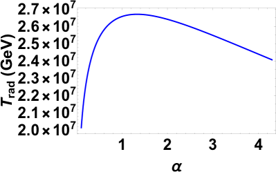
Figure 5: Left panel: The number of e-folds needed to begin the radiation domination at $T=T_{\mathrm{rad}}$. Right panel: The dependency of $T_{\mathrm{rad}}$ on $\alpha$ depicts that the radiation domination is found to be prevalent at temperature around $10^{7}$ GeV.

Let $T_{\mathrm{rad}}$ be attained at the cost of $N(T_{\mathrm{rad}})$ number of e-folds, then from Eqs. (14) and (43)

$$N(T_{\mathrm{rad}})=\ln{\left(\frac{T_{\mathrm{end}}}{T_{\mathrm{rad}}}\right)}=\frac{1}{2}\ln{\left(\frac{12\pi^{3}}{g^{2}}\right)}=12.1698.$$ (48)

Therefore the radiation begins to dominate for the potential considered in Eq. (39) exactly at $12.1698$ e-folds after inflation at the temperature around $10^{7}$ GeV (see figure 5). Interestingly, this result matches with the one at the ‘crossing point’ of energy densities in figure 2 corresponding to the model considered here.

Up to now, it is easily realizable that, SB would occur at any temperature between $\sim 10^{11}-10^{7}$ GeV with the number of e-folds lying in the range $1.69-12.17$. However, the exact value of this temperature can be estimated from the freeze-out temperature $T_{F}$, which is linked with the BTER, calculated in next sub-section.

To get a rough estimate of $T_{F}$, if we assume that at the freeze-out point $\eta_{F}$ is equal to the experimental value $\eta=8.6\times 10^{-11}$ in Eq. (38), $\frac{\lambda^{\prime}M_{p}}{M}$ is restricted between $1$ and $8$ according to Carroll bound, say, $\frac{\lambda^{\prime}M_{p}}{M}=5$ and $T_{\mathrm{th}}=7.5\times 10^{11}$ GeV, taken from figure 4, then within the model concerned $T_{F}$ can be calculated to be $2.28\times 10^{8}$ GeV, which is above $T_{\mathrm{rad}}$ ($\sim 10^{7}$ GeV, see figure 5). Now, in the next sub-section it will be interesting to look at the conditions in which $T_{F}$ acquires the value of this order.

IV.3 Calculations of $T_{F}$ and $\eta_{F}$

In order to compute the freeze-out temperature $T_{F}$, we consider a $B$-violating and $(B-L)$-conserving process, of which the rate, derived from an SM four-fermion non-renormalizable point interaction [47, 10, 50, 52, 75], can be written as,

$$\Gamma_{B-L}(T)=\frac{\bar{g}^{2}}{\tilde{M}^{4}}T^{5},$$ (49)

where $\bar{g}<1$ is the coupling constant and $\tilde{M}$ indicates the effective cut-off of the said interaction. At the specific temperature, $T_{F}$, the rate $\Gamma_{B-L}$ becomes of the same order as that of the Hubble expansion rate $H_{\mathrm{kin}}$ of the universe i.e. $\Gamma_{B-L}(T_{F})\sim H_{\mathrm{kin}}(T_{F})$ (called the freeze-out condition) and beyond that no $B$-violation takes place. Consequently, the baryon number saturates at the freeze-out value. Now, using Eqs. (2), (10) and (49), we obtain

$$T_{F}=\frac{H_{\mathrm{end}}^{1/2}\tilde{M}^{2}}{T_{\mathrm{end}}^{3/2}\bar{g}}.$$ (50)

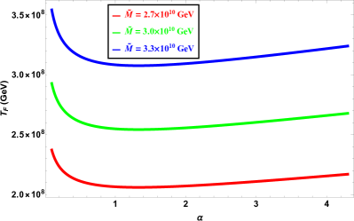
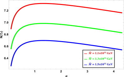
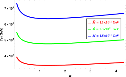
Figure 6: Left column: Number of e-folds elapsed to attain the freezing of baryon non-conserving process at different mass scales. Right column: The variations of freeze-out temperatures with $\alpha$ show that, freezing happens at $\sim 10^{8}-10^{9}$ GeV for a given value of $\tilde{M}$ and $\bar{g}=0.8$. For a particular value of $\alpha$, larger value of number of e-folds corresponds to smaller value of $T_{F}$, which is consistent with the evolution of temperature of the universe with its expansion, described in previous sub-section. With the increase of the mass scale $\tilde{M}$, the number of e-folds decreases and $T_{F}$ increases for a given value of $\alpha$, which are also clear from Eqs. (50) and (51).

The required number of e-folds to reach the temperature $T_{F}$ can be calculated from Eqs. (10) and (43) (as done before in the cases of $N(T_{\mathrm{th}})$ and $N(T_{\mathrm{rad}})$) as,

$$N(T_{F})=\ln{\left(\frac{T_{\mathrm{end}}}{T_{F}}\right)}.$$ (51)

In figure 6 the freeze-out temperature $T_{F}$ (see Eq. (50)) and the corresponding number of e-folds $N(T_{F})$ are plotted as functions of $\alpha$ for various values of the mass-scale $\tilde{M}$. Here, $\tilde{M}$ is so chosen that $T_{F}$ could lie between $T_{\mathrm{th}}$ ($\sim 10^{11}$ GeV) and $T_{\mathrm{rad}}$ ($\sim 10^{7}$ GeV), as stated in previous sub-section. Figure 6 highlights that, depending upon the values of $\tilde{M}$, the freezing of $B$-violating process occurs at a temperature around $10^{8}-10^{9}$ GeV when the universe has covered $6.3-10.2$ number of e-folds, which lie in the midst of thermalization and radiation domination.

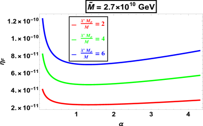
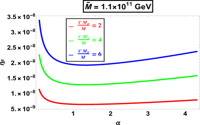
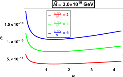
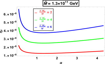
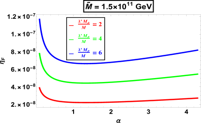
Figure 7: Variations of freeze-out values of BTER with $\alpha$ for three values of $M$ and two sets of values of $\tilde{M}$ corresponding to $\sim 10^{10}$ GeV and $\sim 10^{11}$ GeV. For a particular values of $\alpha$ and $\tilde{M}$, $\eta_{F}$ decreases with the increase in $M$. Similarly, for a particular values of $\alpha$ and $M$, $\eta_{F}$ increases with the increase in $\tilde{M}$.

Finally the task is to estimate the freeze-out value of BTER, $\eta_{F}$, from Eq. (38). To compute the $\eta_{F}$ as function of $\alpha$, three values of $M$ viz., $M=\lambda^{\prime}M_{p}/2=1.2\times 10^{18}$ GeV, $\lambda^{\prime}M_{p}/4=6.07\times 10^{17}$ GeV, $\lambda^{\prime}M_{p}/6=4.05\times 10^{17}$ GeV for $\lambda^{\prime}\approx 1$ and the estimated values of $T_{\mathrm{th}}$ and $T_{F}$ shown in figures 4 and 6, respectively, have been considered. The choices of $\tilde{M}$ remains the same as shown in figure 6. Two sets of $\tilde{M}$, each containing three values, corresponding to $\tilde{M}\sim 10^{10}$ GeV and $\tilde{M}\sim 10^{11}$ GeV are taken into account.

In figure 7, the obtained values of $\eta_{F}$ with the variation of $\alpha$ from $\alpha=0.1$ to $\alpha=4.3$ are shown. The left column corresponds to the variations when $\tilde{M}\sim 10^{10}$ GeV and the right column comprises that for $\tilde{M}\sim 10^{11}$ GeV. The results show that the cut-off scale $M$ has no such significant effects, where as, $\tilde{M}$ affects $\eta_{F}$ significantly. When $\tilde{M}\sim 10^{10}$ GeV, $\eta_{F}$ is of the order of $10^{-10}-10^{-11}$, which is required for obtaining the experimental bound. Similarly, when $\tilde{M}\sim 10^{11}$ GeV, $\eta_{F}$ is of the order of $10^{-7}-10^{-9}$, which is higher than that of the experimental bound.

For $\tilde{M}=2.7\times 10^{10}$ GeV and $M=4.05\times 10^{17}$ GeV (see the blue curve of the first plot in left column of figure 7), two ranges of values of $\eta_{F}$ are found to be closest to the experimental value, $\eta\approx(8.6\pm 0.1)\times 10^{-11}$. They are $\eta_{F}=8.7\times 10^{-11}-8.5\times 10^{-11}$ for $\alpha=0.29-0.3$ respectively and $\eta_{F}=8.5\times 10^{-11}-8.6\times 10^{-11}$ for $\alpha=4.2-4.3$ respectively. Therefore, there exists two ranges viz., $\alpha=0.29-0.3$ and $\alpha=4.2-4.3$ corresponding to the lower and upper ends of $\alpha$, respectively, in which the calculated BTER satisfies the experimental value with specified error bar for the mass scales $\tilde{M}=2.7\times 10^{10}$ GeV and $M=4.05\times 10^{17}$ GeV.

Table 1: Calculate values of $\eta_{F}$, $T_{\mathrm{th}}$ and $T_{F}$ for two ranges of values of $\alpha$, where $\eta_{F}$ satisfies the experimental requirement: $\eta\approx(8.6\pm 0.1)\times 10^{-11}$.

$\alpha$	$\eta_{F}/(10^{-11})$	$T_{\mathrm{th}}/(10^{11})$	$T_{F}/(10^{8})$	$\frac{T_{\mathrm{th}}}{T_{F}}\times 10^{-3}$
$0.29-0.3$	$8.7-8.5$	$7.78-7.79$	$2.175-2.17$	$3.577-3.59$
$4.2-4.3$	$8.5-8.6$	$7.83-7.81$	$2.15-2.17$	$3.642-3.599$

Table 1 shows that, in the regime, where $\eta_{F}$ satisfies the experimental value, the maximum thermalization temperature is found to be $T_{\mathrm{th}}=7.78\times 10^{11}-7.79\times 10^{11}$ GeV for $\alpha=0.29-0.3$ and $T_{\mathrm{th}}=7.83\times 10^{11}-7.81\times 10^{11}$ GeV for $\alpha=4.2-4.3$ (see figure 4). Similarly, the freeze-out temperature is obtained as $T_{F}=2.175\times 10^{8}-2.17\times 10^{8}$ GeV for $\alpha=0.29-0.3$ and $T_{F}=2.15\times 10^{8}-2.17\times 10^{8}$ GeV for $\alpha=4.2-4.3$ (see the red curve in the first plot of second column of figure 6). Here, $T_{\mathrm{th}}/T_{F}=3.577\times 10^{3}-3.59\times 10^{3}$ for $\alpha=0.29-0.3$ and $T_{\mathrm{th}}/T_{F}=3.642\times 10^{3}-3.599\times 10^{3}$ for $\alpha=4.2-4.3$, which are close to the value given in Ref. [50]. In these two ranges of $\alpha$, the temperature at the end of inflation (or the start of kination) $T_{\mathrm{end}}$ and the temperature of radiation domination, $T_{\mathrm{rad}}$, are obtained as, $T_{\mathrm{end}}=4.60\times 10^{12}-4.65\times 10^{12}$ GeV, $T_{\mathrm{rad}}=2.38\times 10^{7}-2.39\times 10^{7}$ GeV for $\alpha=0.29-0.3$ and $T_{\mathrm{end}}=4.66\times 10^{12}-4.63\times 10^{12}$ GeV, $T_{\mathrm{rad}}=2.42\times 10^{7}-2.4\times 10^{7}$ GeV for $\alpha=4.2-4.3$ (see figures 3 and 5). Also, the symmetry breaking scale $M$ ($\sim 10^{17}$ GeV) is found to be $10^{5}$ times larger than the Hubble rate $H_{\mathrm{end}}$ ($\sim 10^{12}$ GeV) (see figure 3), which is an important result according to Ref. [4].

Thus, from all the analyses done so far, it can be said that, for the potential concerned in Eq. (39) the SB takes place at the temperature $T$ lying within the following inequality

$$\begin{split}&T_{\mathrm{rad}}(\sim 10^{7}\mathrm{GeV})<T_{F}(\sim 10^{8}\mathrm{GeV})<T(\mathrm{GeV})\\ &<T_{\mathrm{th}}(\sim 10^{11}\mathrm{GeV})<T_{\mathrm{end}}(\sim 10^{12}\mathrm{GeV})\\ &<M(\sim 10^{17}\mathrm{GeV})<M_{p}(\sim 10^{18}\mathrm{GeV}).\end{split}$$ (52)

IV.4 Spectra of the relic gravitational waves

Gravitational waves (GWs) are the results of tensor perturbations in spatially-flat FLRW metric defined by (written in standard notations) [77]

$$ds^{2}=-dt^{2}+a^{2}(t)\left(\delta_{mn}+h_{mn}\right)dx^{m}dx^{n}.$$ (53)

$h_{mn}$ are the metric perturbations, which are transverse ($\partial_{m}h_{mn}=0$) having two crossed polarization states and trace-less ($h_{mm}=0$). The root-mean-square (RMS) value of the amplitudes of the GW spectrum, $\Omega_{GW}(k,\tau)$, is measured as the ratio of logarithmic derivative of GW energy density $\rho_{GW}$ with respect to the mode $k$ and the conformal time ($\tau$)-dependent critical energy density $\rho_{c}=3M_{p}^{2}H^{2}(\tau)$ [65, 52]. This can be transferred to its present-day value $\Omega_{GW,0}$ [65, 52] by extracting the effects of (dimensionless) inflationary tensor power spectrum $\Delta^{2}_{h}(k)$ (see [80] for the calculations of mode-dependent tensor power spectrum) at present-day, through a transfer function $T_{\mathrm{trans}}^{2}(k,\tau)$ [81, 82, 83]. This function encodes the post-inflationary evolution of a mode $k$ from horizon re-entry to time ($\tau$) of observation. Now, a number of expressions of $\Omega_{GW,0}$ exist depending upon the various epochs in which the modes re-enter the horizon. Among them, only the kinetic-dominated (KD) and radiation-dominated (RD) epochs are the subjects of interest in the present work. They are given by [76, 65, 50, 52, 84],

$$\Omega^{(\mathrm{RD})}_{GW,0}(k)=\left(\frac{\Omega_{\mathrm{rad},0}}{6\pi^{2}}\right)\left(\frac{H_{\mathrm{inf}}^{2}}{M_{p}^{2}}\right)\left(\frac{g_{*}}{g_{*,0}}\right)\left(\frac{g_{*s,0}}{g_{*s}}\right)^{4/3}$$ (54)

for $k_{\mathrm{equal}}<k\leq k_{\mathrm{rad}}$ and

$$\Omega^{(\mathrm{KD})}_{GW,0}(k)=\Omega^{(\mathrm{RD})}_{GW,0}(k)\left(\frac{k}{k_{\mathrm{rad}}}\right)$$ (55)

for $k_{\mathrm{rad}}<k\leq k_{\mathrm{end}}$. $\Omega_{\mathrm{rad},0}=9.13\times 10^{-5}$ [79, 78] is the present-day density parameter of radiation. $g_{*s}$ and $g_{*}$ are relativistic degrees of freedom corresponding to entropy density and radiation density respectively, which are of the same order i.e. $10^{2}$ [52]. $g_{*s,0}=3.91$ and $g_{*,0}=3.36$ are their present values [79, 78]. The subscripts ‘end’, ‘rad’ and ‘equal’ in $k$ refer to the modes taking re-entry during the end of inflation (or start of kination), radiation era and matter-radiation equality, respectively. Here, $H_{\mathrm{inf}}$ refers to the inflationary Hubble parameter which is generically mode-dependent (see Ref. [80]) and hence a little complicated. But it can be simplified for the plateau-type potential considered here (see Eq. (39)), for which tensor-to-scalar ratio is small, by approximating $H_{\mathrm{inf}}\approx H_{\mathrm{end}}$, which is $k$-independent. Therefore the GW spectrum during the radiation era is roughly scale-independent. It depends only on $\alpha$ through $H_{\mathrm{end}}$, while that for kinetic domination is slightly blue-tilted, which will be examined in the next paragraph. In figure 8, we plot the RMS values of the amplitudes of the present-day RD-GW spectrum against $\alpha$, and the results show that they are $\sim 10^{-18}$, which is indeed very small, lying within the projected ranges of various ongoing experiments (see figure 11). The corresponding peak value [65, 52, 50] is given by,

$$\left(\Omega^{RD}_{GW,0}\right)_{\mathrm{peak}}=\Omega^{RD}_{GW,0}\left(\frac{T_{\mathrm{end}}}{T_{\mathrm{rad}}}\right)^{2}.$$ (56)

In figure 9 the peak values of amplitudes of present-day RD-GW spectrum are plotted against $\alpha$, in which the peak values are found to be $\sim 10^{-7}$, which satisfy the following constraint of BBN [66, 67]

$$\left(\Omega^{RD}_{GW,0}\right)_{\mathrm{peak}}<2.46\times 10^{-6}.$$ (57)

For $\alpha=0.29-0.3$ we get $\Omega^{(\mathrm{RD})}_{GW,0}=3.14\times 10^{-18}-3.2\times 10^{-18}$ and $\left(\Omega^{RD}_{GW,0}\right)_{\mathrm{peak}}=1.16\times 10^{-7}-1.2\times 10^{-7}$. Similarly, for $\alpha=4.2-4.3$ we obtain $\Omega^{(\mathrm{RD})}_{GW,0}=3.3\times 10^{-18}-3.23\times 10^{-18}$ and $\left(\Omega^{RD}_{GW,0}\right)_{\mathrm{peak}}=1.22\times 10^{-7}-1.2\times 10^{-7}$.

Therefore, the potential considered in Eq. (39) is viable in making a reliable connection between the GeV-scale - (spontaneous) baryogenesis and the BBN.

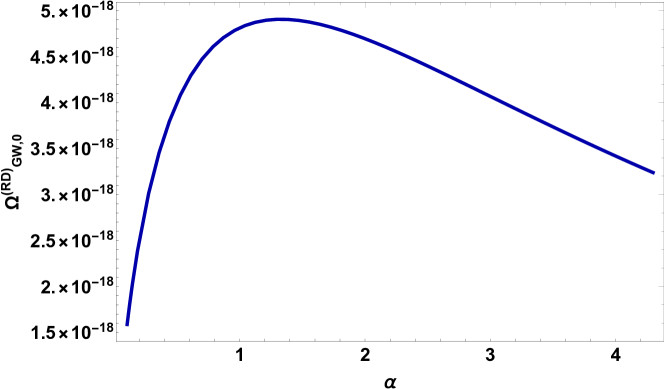
Figure 8: Plot of the RMS values of the amplitudes for the present-day RD-GW spectrum against $\alpha$.

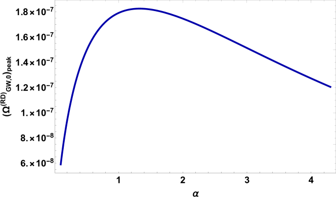
Figure 9: Plot of the peak values of the amplitudes for the present-day RD-GW spectrum against $\alpha$.

The GW frequencies [76, 65] having wave vectors $k_{\mathrm{rad}}$ and $k_{\mathrm{end}}$ indicated in Eqs. (54) and (55) can be calculated using,

$$f_{\mathrm{rad}}=1600\times\left(\frac{T_{\mathrm{rad}}}{10^{10}\mathrm{GeV}}\right)\mathrm{Hz}$$ (58)

and

$$f_{\mathrm{end}}=8900\times\left(\frac{H_{\mathrm{inf}}}{g\times 10^{4}\mathrm{GeV}}\right)^{1/2}\mathrm{Hz}.$$ (59)

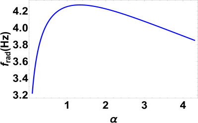
Figure 10: GW frequencies of the modes taking re-entry during radiation domination and the end of inflation (i.e. start of kination).

Figure 10 shows that the obtained values of $f_{\mathrm{end}}$ and $f_{\mathrm{rad}}$ are $\sim 10^{10}$ Hz and $\sim 10^{1}$ Hz respectively. For $\alpha=0.29-0.3$ we get $f_{\mathrm{end}}=2\times 10^{10}-2.1\times 10^{10}$ Hz and $f_{\mathrm{rad}}=3.7-3.78$ Hz. Similarly, for $\alpha=4.2-4.3$ we obtain $f_{\mathrm{end}}=2.12\times 10^{10}-2.11\times 10^{10}$ Hz and $f_{\mathrm{rad}}=3.8-3.78$ Hz. The $f_{\mathrm{end}}$ frequencies are large enough and hence they are often called the blue tilted [85, 65, 50]. Ref. [50] shows that the frequencies of the modes entering the horizon at present and during matter-radiation equality (corresponding to $k_{\mathrm{equal}}$) are of the order of $10^{-19}$ Hz and $10^{-17}$ Hz respectively, for which they are termed as the red tilted.

Therefore, during the transition from inflation to kination GWs of very high frequencies (blue tilted) are emitted. This is because a sharp transition takes place from periods of inflation to kination due to a change of metric structure. Other transitions are smooth for which the corresponding emitted GWs are of low frequencies (red tilted). However, all GWs have very low amplitudes and therefore they are too feeble to detect.

In the present era of precision cosmology and multi-messenger astronomy [86], several ground-based and space-based GW detectors are in operation to detect the GW frequencies from very low end to very high end (see figure 11). For example, Advanced-LIGO [87], Advanced-Virgo [88] and KAGRA [89] detect the GW-strain $\sim 10^{-9}$ at roughly $100$ Hz. Again, the Laser Interferometer Space Antenna (LISA) [90] and Deci-Hertz Interferometer Gravitational-wave Observatory (DECIGO) [91] are made to sense the frequencies approximately from $0.001$ Hz to $\sim 0.1$ Hz. Even weaker GWs of frequency like $\sim 10^{-8}$ Hz can be probed using Square Kilometer Array (SKA) [92], the largest radio telescope, so far.

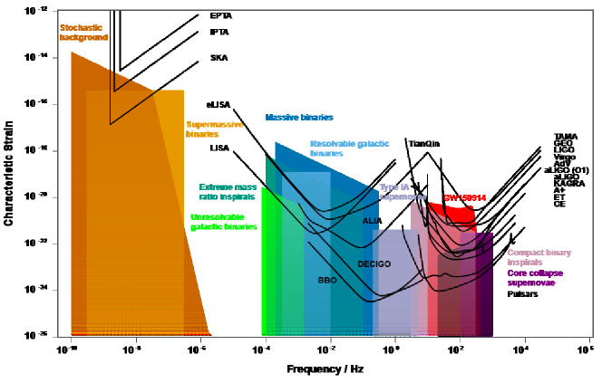
Figure 11: GW sensitivity curves of various detectors from several sources. The plot has been generated on-line using http://gwplotter.com/ based on the Ref. [93].

The stochastic signatures of blue-tilted frequencies are important in probing deeply into the ‘pre-cosmic microwave background scenario’ and therefore validating the paradigm of quintessential inflation, specifically the kination. Unfortunately, at present, no GW detectors are able to detect $\sim 10^{10}$ Hz ($f_{\mathrm{end}}$) frequency. It needs more sensitivity and sophistication. At least it is satisfactory that the frequencies $\sim 10$ Hz ($f_{\mathrm{rad}}$) are being detected in the ongoing experiments.

There is an interesting connection between the GWs and the theory of inflation. Figure 11 shows that every experimental group has observed GWs of strain $\sim 10^{-14}-10^{-24}$, which is undoubtedly too small. It is because, according to Eqs. (4, (15) and (54) the strain is proportional to tensor-to-scalar ratio $r$, which is very small ($<0.064$ [79]) for plateau-type model of inflation. In a previous work [70] for the same potential considered here, the $r$ is found to be $\sim 10^{-4}-10^{-2}$ for $0.1\leq\alpha\leq 4.3$ at the pivot scale $k=0.002$ Mpc^-1. Therefore the observed tiny values of GW-strain indirectly support the framework of slow-roll inflation, just like Planck observation [79]. However, this aspect will be more prominent after the detection of $B$ modes with desired accuracy (see [80, 70] for further discussions).

V Conclusions

In conclusion, we have

1. applied a new model of quintessential $\alpha$-attractor inflaton potential to study the scenario of spontaneous baryogenesis (SB) within $0.1\leq\alpha\leq 4.3$ and $n=122$,

2. studied SB by deriving the expressions of energy density and equation of motion of $\phi$ field, baryon excess and the freeze-out value of baryon-to-entropy ratio (BTER) at finite temperature by incorporating the derivative coupling of $\phi$ field with the non-conserving baryon current with a cut-off scale $M$. This coupling, describing a CP-odd effective interaction, brings extra terms in total field-energy density corresponding to the number densities of particles and anti-particles. By a calculation of statistical phase space distribution, the number density of particles is found to be greater than that of anti-particles for a non-zero value of field velocity, leading to the ‘baryon-excess’ of the universe. This baryon-excess is translated into the computation of BTER. In this course, the effect of back-reaction is shown to be negligible in the dynamical equation of motion of the quintessential inflaton field,

3. examined the evolution during kination of total field density $\rho_{\mathrm{kin}}$ and radiation density $\rho_{\mathrm{rad}}$ of the particles created through instant preheating (IP), with the expansion of the universe, which is measured by the number of e-folds $N$, elapsed after the end of inflation. The two energy densities are found to have same order of magnitude, which is very necessary for a successful BBN process during matter domination (which actually makes the IP a better reheating process rather than GPP). At $N=12.1698$ there exists a cross-over between the above mentioned energy densities, which acts as a transition point between starting and ending of the SB process as well as between the domination of $\phi$-field and radiation,

4. derived the expressions of the temperature, $T_{\mathrm{end}}$ at the end of inflation (or start of kination), the maximum thermalization temperature $T_{\mathrm{th}}$, and the temperature of radiation domination $T_{\mathrm{rad}}$, which have been used to examine the post-inflationary kination period related to SB,

5. analyzed the evolution of these three temperatures and their respective number of e-folds with $\alpha$ within the range specified earlier. The order of magnitude of the values of $T_{\mathrm{th}}$ are close to that of $T_{\mathrm{end}}$ and too far from that of $T_{\mathrm{rad}}$ signifying the fact that, thermal equilibrium attains just after the end of inflation and long before the beginning of radiation era. This is needed to set a perfect stage for the BBN in matter dominated era; because, even a slight deviation of the order of the values of the said temperatures could be threatening for obtaining the observed constraints of BBN,

6. considered an effective non-renormalizable $4$-fermion point interaction with a cut-off scale $\tilde{M}$ and the associated rate of $B$-violation $\Gamma_{B-L}$ to compute the freeze-out temperature $T_{F}$ and the baryon-to-entropy ratio $\eta_{F}$ with the variations of $\alpha$ for fixed values of $M$ and $\tilde{M}$ using the ‘freeze-out condition’. The obtained values of $T_{F}$ lie in between $T_{\mathrm{th}}$ and $T_{\mathrm{rad}}$ and much below the cut-off mass-scale $\tilde{M}$, required for implementing the effective $4$-fermi construct method. The ratio $T_{\mathrm{th}}/T_{F}$ becomes consistent with the value given in the current literature. On the other hand, the $\eta_{F}$ values conform to the experimental bound for two narrow ranges of $\alpha$ viz., $\alpha=0.29-0.3$ and $4.2-4.3$ and the specific values of $M(\sim 10^{17}\leavevmode\nobreak\ \mathrm{GeV})$ and $\tilde{M}(\sim 10^{10}\leavevmode\nobreak\ \mathrm{GeV})$. In between these two ranges of $\alpha$, the values of $\eta_{F}$ slightly deviate from the experimental value, keeping the order of magnitude same, and

7. studied the variations of the amplitudes and the frequencies of the spectra of relic gravitational waves with $\alpha$ for two types of transitions - one is from inflation to kination ($KD$) and another is from $\phi$ domination to radiation domination ($RD$). The calculated magnitudes of the present-day RMS values of $RD-GW$ amplitudes, $\Omega_{GW,0}^{(\mathrm{RD})}$, are consistent with the sensitivity profile of the ongoing $GW$-detectors. The corresponding peak values, $(\Omega_{GW,0}^{(\mathrm{RD})})_{\mathrm{peak}}$, satisfy the BBN constraint quite satisfactorily. A blue tilted $KD-GW$ spectrum is also found to exist, which is an essential feature of the model of quintessential inflation in the context of SB.

The new model of quintessential $\alpha$-attractor inflaton potential, considered in this paper, therefore, appears to be efficacious in explaining the baryon asymmetry at GeV-scale in the light of current cosmological surveys and generation of ‘blue-spectrum’ of relic gravitational waves for $\alpha=0.29-0.3$ and $\alpha=4.2-4.3$. According to Ref. [70], this model is equally efficient in explaining early and late-time expansions of the universe for $0.1\leq\alpha\leq 4.3$. Therefore, the combined results of the present paper and Ref. [70] show that, the concerned potential is capable of unifying inflation, baryogenesis and quintessence in a single framework.

Appendix A Density of $\phi$ field with the effective interaction

The Lagrangian of the $\phi$-field is given by

$$\mathcal{L}_{\phi}=-\frac{1}{2}g^{\beta\gamma}\partial_{\beta}\phi\partial_{\gamma}\phi-V(\phi)-\frac{\lambda^{\prime}}{M}\partial_{\beta}\phi J^{\beta}$$ (60)

and the corresponding energy-momentum tensor can be calculated as

$$\begin{split}T_{\nu}^{\mu}&=\delta_{\nu}^{\mu}\mathcal{L}_{\phi}-2g^{\mu\alpha}\frac{\partial\mathcal{L}_{\phi}}{\partial g^{\alpha\nu}}\\ &=\delta_{\nu}^{\mu}\left(-\frac{1}{2}g^{\beta\gamma}\partial_{\beta}\phi\partial_{\gamma}\phi-V(\phi)-\frac{\lambda^{\prime}}{M}\partial_{\beta}\phi J^{\beta}\right)\\ &+\left(g^{\mu\alpha}\partial_{\alpha}\phi\partial_{\nu}\phi+\frac{2\lambda^{\prime}}{M}g^{\mu\alpha}\partial_{\alpha}\phi J_{\nu}\right)\\ &=\delta_{\nu}^{\mu}\left(\frac{\dot{\phi}^{2}}{2}-V(\phi)-\frac{\lambda^{\prime}}{M}\dot{\phi}J^{0}\right)\\ &+\left(g^{\mu 0}\dot{\phi}\partial_{\nu}\phi+\frac{2\lambda^{\prime}}{M}g^{\mu 0}\dot{\phi}J_{\nu}\right).\end{split}$$ (61)

The time-time component of $T_{\nu}^{\mu}$ is,

$$\begin{split}T_{0}^{0}&=\left(\frac{\dot{\phi}^{2}}{2}-V(\phi)-\frac{\lambda^{\prime}}{M}\dot{\phi}J^{0}\right)+\left(-\dot{\phi}^{2}+\frac{2\lambda^{\prime}}{M}\dot{\phi}J^{0}\right)\\ &=-\frac{\dot{\phi}^{2}}{2}-V(\phi)+\frac{\lambda^{\prime}}{M}\dot{\phi}J^{0},\end{split}$$ (62)

from which we obtain the density as

$$\begin{split}\rho&=-T_{0}^{0}=\frac{\dot{\phi}^{2}}{2}+V(\phi)-\frac{\lambda^{\prime}}{M}\dot{\phi}J^{0}\\ &=\frac{\dot{\phi}^{2}}{2}+V(\phi)-\frac{\lambda^{\prime}}{M}\dot{\phi}\left(n-\bar{n}\right).\end{split}$$ (63)

Appendix B Derivation of baryon excess $\Delta n$

The Fermi-Dirac distribution function for massless relativistic baryons having momentum $|\vec{p}|\equiv p$, energy $\epsilon=p$ and chemical potential $\mu$ is,

$$f(p,\mu)=\frac{1}{e^{\left(\frac{p-\mu}{T}\right)}+1}=\frac{e^{-p/T}}{e^{-\mu/T}+e^{-p/T}}.$$ (64)

Under high temperature approximation we have $\mu/T\ll 1$ and terms $\mathcal{O}(\mu^{2}/T^{2})$ are neglected. Therefore,

$$\begin{split}&f(p,\mu)\approx\frac{e^{-p/T}}{1-\left(\frac{\mu}{T}-e^{-p/T}\right)}\\ &=e^{-p/T}\left[1-\left(\frac{\mu}{T}-e^{-p/T}\right)\right]^{-1}\\ &=e^{-p/T}\left[1+\sum_{\mathbb{Z}\ni n=1}^{\infty}\left(\frac{\mu}{T}-e^{-p/T}\right)^{n}\right]\\ &=e^{-p/T}\Bigl{[}1+\sum_{\mathbb{Z}\ni n=1}^{\infty}\sum_{m=0}^{n}{}^{n}C_{m}\left(\frac{\mu}{T}\right)^{n-m}\left(-e^{-p/T}\right)^{m}\Bigr{]}\\ &\approx e^{-p/T}\left[1+\sum_{\mathbb{Z}\ni n=1}^{\infty}{}^{n}C_{n-1}\left(\frac{\mu}{T}\right)\left(-e^{-p/T}\right)^{n-1}\right]\\ &=e^{-p/T}+\frac{\mu}{T}\sum_{\mathbb{Z}\ni n=1}^{\infty}n\left(-1\right)^{n-1}\left(e^{-np/T}\right).\end{split}$$ (65)

Similarly, the same distribution function for anti-baryons is

$$f(p,-\mu)=e^{-p/T}-\frac{\mu}{T}\sum_{\mathbb{Z}\ni n=1}^{\infty}n\left(-1\right)^{n-1}\left(e^{-np/T}\right).$$ (66)

Therefore,

$$f(p,\mu)-f(p,-\mu)=\frac{2\mu}{T}\sum_{\mathbb{Z}\ni n=1}^{\infty}n\left(-1\right)^{n-1}\left(e^{-np/T}\right).$$ (67)

Thus, the baryon excess,

$$\begin{split}&\Delta n=n-\bar{n}=\int\tilde{g}\frac{d^{3}\vec{p}}{(2\pi)^{3}}\left[f(p,\mu)-f(p,-\mu)\right]\\ &=\int_{0}^{\infty}\tilde{g}\frac{4\pi p^{2}dp}{(2\pi)^{3}}\left[f(p,\mu)-f(p,-\mu)\right]\\ &=\tilde{g}\frac{\mu}{\pi^{2}T}\sum_{\mathbb{Z}\ni n=1}^{\infty}n(-1)^{n-1}\int_{0}^{\infty}p^{2}e^{-np/T}dp.\end{split}$$ (68)

Putting $x=\frac{np}{T}$,

$$\begin{split}&\Delta n=\tilde{g}\frac{\mu T^{2}}{\pi^{2}}\sum_{\mathbb{Z}\ni n=1}^{\infty}\frac{(-1)^{n-1}}{n^{2}}\int_{0}^{\infty}x^{2}e^{-x}dx\\ &=\tilde{g}\frac{\mu T^{2}}{\pi^{2}}\eta(2)\Gamma(3),\end{split}$$ (69)

where $\eta(2)$ is the Dirichlet eta function, which is related to Riemann zeta function as $\eta(2)=\left(1-2^{1-2}\right)\zeta(2)$. Putting $\zeta(2)=\frac{\pi^{2}}{6}$ and $\Gamma(3)=2!$ we finally obtain

$$\Delta n=\frac{\tilde{g}\mu T^{2}}{6}=\frac{\tilde{g}\lambda^{\prime}\dot{\phi}T^{2}}{6M}.$$ (70)

Appendix C Equation of motion of $\phi$ with the effective interaction

We have the Lagrangian for the $\phi$ field

$$\mathcal{L}_{\phi}=-\frac{1}{2}g^{\beta\gamma}\partial_{\beta}\phi\partial_{\gamma}\phi-V(\phi)-\frac{\lambda^{\prime}}{M}\partial_{\beta}\phi J^{\beta},$$ (71)

where the metric is composed of usual Friedmann metric components $g_{00}=-1$ and $g_{ii}=a^{2}$ such that $\sqrt{-g}=a^{3}$. Now,

$$\begin{split}&\frac{\partial\mathcal{L}_{\phi}}{\partial(\partial_{\mu}\phi)}=-\frac{1}{2}g^{\beta\gamma}\left(\delta_{\beta}^{\mu}\partial_{\gamma}\phi+\partial_{\beta}\phi\delta_{\gamma}^{\mu}\right)-\frac{\lambda^{\prime}}{M}\delta_{\beta}^{\mu}J^{\beta}\\ &=-g^{\mu\beta}\partial_{\beta}\phi-\frac{\lambda^{\prime}}{M}\delta_{\beta}^{\mu}J^{\beta}=-g^{\mu 0}\dot{\phi}-\frac{\lambda^{\prime}}{M}\delta_{0}^{\mu}J^{0},\end{split}$$ (72)

$$\begin{split}&\partial_{\mu}\left(\sqrt{-g}\frac{\partial\mathcal{L}_{\phi}}{\partial(\partial_{\mu}\phi)}\right)\\ &=-\frac{\partial_{\mu}g}{2\sqrt{-g}}\frac{\partial\mathcal{L}_{\phi}}{\partial(\partial_{\mu}\phi)}+\sqrt{-g}\partial_{\mu}\left(\frac{\partial\mathcal{L}_{\phi}}{\partial\left(\partial_{\mu}\phi\right)}\right)\\ &=\frac{6a^{5}\dot{a}}{2a^{3}}\left(\dot{\phi}-\frac{\lambda^{\prime}}{M}J^{0}\right)+a^{3}\left(\ddot{\phi}-\frac{\lambda^{\prime}}{M}\partial_{0}J^{0}\right)\\ &=a^{3}\left[\left(\ddot{\phi}-\frac{\lambda^{\prime}}{M}\partial_{0}J^{0}\right)+3H\left(\dot{\phi}-\frac{\lambda^{\prime}}{M}J^{0}\right)\right]\\ &=a^{3}\left[\left(\ddot{\phi}-\frac{\tilde{g}\lambda^{\prime 2}T^{2}}{6M^{2}}\ddot{\phi}\right)+3H\left(\dot{\phi}-\frac{\tilde{g}\lambda^{\prime 2}T^{2}}{6M^{2}}\dot{\phi}\right)\right]\\ &=a^{3}\left[1-\frac{\tilde{g}}{6}\left(\frac{\lambda^{\prime}M_{p}}{M}\right)^{2}\left(\frac{T}{M_{p}}\right)^{2}\right]\left(\ddot{\phi}+3H\dot{\phi}\right)\end{split}$$ (73)

and

$$\frac{\partial\left(\sqrt{-g}\mathcal{L}_{\phi}\right)}{\partial\phi}=-a^{3}\frac{\partial V}{\partial\phi}.$$ (74)

Therefore, the equation of motion becomes

$$\begin{split}&\left[\partial_{\mu}\left(\frac{\partial}{\partial(\partial_{\mu}\phi)}\right)-\frac{\partial}{\partial\phi}\right]\sqrt{-g}\mathcal{L}_{\phi}=0\\ \mathrm{or,}&\left[1-\frac{\tilde{g}}{6}\left(\frac{\lambda^{\prime}M_{p}}{M}\right)^{2}\left(\frac{T}{M_{p}}\right)^{2}\right]\left(\ddot{\phi}+3H\dot{\phi}\right)+\frac{\partial V}{\partial\phi}=0.\end{split}$$ (75)

References

- [1] J. M. Cline, “Baryogenesis,” in Les Houches Summer School - Session 86: Particle Physics and Cosmology: The Fabric of Spacetime. 9, 2006. arXiv:hep-ph/0609145.
- [2] S. Aharony Shapira, “Current bounds on baryogenesis from complex Yukawa couplings of light fermions,” Phys. Rev. D 105 no. 9, (2022) 095037, arXiv:2106.05338 [hep-ph].
- [3] V. A. Rubakov, “Cosmology and dark matter,” CERN Yellow Rep. School Proc. 5 (2022) 129, arXiv:1912.04727 [hep-ph].
- [4] A. De Simone and T. Kobayashi, “Cosmological Aspects of Spontaneous Baryogenesis,” JCAP 08 (2016) 052, arXiv:1605.00670 [hep-ph].
- [5] A. D. Sakharov, “Violation of CP Invariance, C asymmetry, and baryon asymmetry of the universe,” Pisma Zh. Eksp. Teor. Fiz. 5 (1967) 32–35.
- [6] M. Quiros, “Finite temperature field theory and phase transitions,” in ICTP Summer School in High-Energy Physics and Cosmology, pp. 187–259. 1, 1999. arXiv:hep-ph/9901312.
- [7] P. B. Arnold and L. D. McLerran, “Sphalerons, Small Fluctuations and Baryon Number Violation in Electroweak Theory,” Phys. Rev. D 36 (1987) 581.
- [8] F. R. Klinkhamer and N. S. Manton, “A Saddle Point Solution in the Weinberg-Salam Theory,” Phys. Rev. D 30 (1984) 2212.
- [9] B. Ghosh, “Electroweak phase transition and some related phenomena – a brief review,” Pramana 87 no. 3, (2016) 43, arXiv:1507.01576 [hep-ph].
- [10] M. Trodden, “Baryogenesis and the new cosmology,” Pramana 62 (2004) 451–464, arXiv:hep-ph/0302151.
- [11] S. Aziz, B. Ghosh, and G. Dey, “Broken electroweak phase at high temperature in the Littlest Higgs model with T-parity,” Phys. Rev. D 79 (2009) 075001, arXiv:0901.3442 [hep-ph].
- [12] S. Aziz and B. Ghosh, “On electroweak baryogenesis in the littlest Higgs model with T parity,” Mod. Phys. Lett. A 27 (2012) 1250190, arXiv:1007.0485 [hep-ph].
- [13] E.-M. Ilgenfritz, J. Kripfganz, H. Perlt, and A. Schiller, “3-d lattice simulation of the electroweak phase transition at small Higgs mass,” Phys. Lett. B 356 (1995) 561–566, arXiv:hep-lat/9506023.
- [14] M. Gurtler, E.-M. Ilgenfritz, J. Kripfganz, H. Perlt, and A. Schiller, “Three-dimensional lattice studies of the electroweak phase transition at M (Higgs) approximates 70-GeV,” Nucl. Phys. B 483 (1997) 383–415, arXiv:hep-lat/9605042.
- [15] K. Kajantie, M. Laine, K. Rummukainen, and M. E. Shaposhnikov, “A Nonperturbative analysis of the finite T phase transition in SU(2) x U(1) electroweak theory,” Nucl. Phys. B 493 (1997) 413–438, arXiv:hep-lat/9612006.
- [16] LEP Working Group for Higgs boson searches, ALEPH, DELPHI, L3, OPAL Collaboration, R. Barate et al., “Search for the standard model Higgs boson at LEP,” Phys. Lett. B 565 (2003) 61–75, arXiv:hep-ex/0306033.
- [17] DELPHI Collaboration, J. Abdallah et al., “Final results from DELPHI on the searches for SM and MSSM neutral Higgs bosons,” Eur. Phys. J. C 32 (2004) 145–183, arXiv:hep-ex/0303013.
- [18] ATLAS Collaboration, G. Aad et al., “Observation of a new particle in the search for the Standard Model Higgs boson with the ATLAS detector at the LHC,” Phys. Lett. B 716 (2012) 1–29, arXiv:1207.7214 [hep-ex].
- [19] CMS Collaboration, S. Chatrchyan et al., “Observation of a New Boson at a Mass of 125 GeV with the CMS Experiment at the LHC,” Phys. Lett. B 716 (2012) 30–61, arXiv:1207.7235 [hep-ex].
- [20] A. G. Cohen and D. B. Kaplan, “Thermodynamic Generation of the Baryon Asymmetry,” Phys. Lett. B 199 (1987) 251–258.
- [21] A. G. Cohen and D. B. Kaplan, “SPONTANEOUS BARYOGENESIS,” Nucl. Phys. B 308 (1988) 913–928.
- [22] A. G. Cohen, D. B. Kaplan, and A. E. Nelson, “Spontaneous baryogenesis at the weak phase transition,” Phys. Lett. B 263 (1991) 86–92.
- [23] S. A. Abel, W. N. Cottingham, and I. B. Whittingham, “Spontaneous baryogenesis in supersymmetric models,” Nucl. Phys. B 410 (1993) 173–187, arXiv:hep-ph/9212299.
- [24] L. Reina and M. Tytgat, “Spontaneous baryogenesis with observable CP violation,” Phys. Rev. D 50 (1994) 751–757, arXiv:hep-ph/9307212.
- [25] D. Comelli, M. Pietroni, and A. Riotto, “Linear response theory approach to spontaneous baryogenesis,” Astropart. Phys. 4 (1995) 71–86, arXiv:hep-ph/9406369.
- [26] J. McDonald, “A Simple estimate of the effect of diffusion on the baryon number generated in spontaneous baryogenesis models,” Phys. Lett. B 353 (1995) 267–273. [Erratum: Phys.Lett.B 364, 246 (1995)].
- [27] D. Comelli, M. Pietroni, and A. Riotto, “Particle currents on a CP violating Higgs background and the spontaneous baryogenesis mechanism,” Phys. Lett. B 354 (1995) 91–98, arXiv:hep-ph/9504265.
- [28] A. D. Dolgov, “Baryogenesis, 30 years after,” in 25th ITEP Winter School of Physics. 7, 1997. arXiv:hep-ph/9707419.
- [29] F. Takahashi and M. Yamaguchi, “Spontaneous baryogenesis in flat directions,” Phys. Rev. D 69 (2004) 083506, arXiv:hep-ph/0308173.
- [30] R. H. Brandenberger and M. Yamaguchi, “Spontaneous baryogenesis in warm inflation,” Phys. Rev. D 68 (2003) 023505, arXiv:hep-ph/0301270.
- [31] B. Feng, “Spontaneous Baryogenesis, CPT Violations and the Observational Imprints,” in 16th Workshop on General Relativity and Gravitation, pp. 22–25. 2006.
- [32] F. Takahashi and M. Yamada, “Spontaneous Baryogenesis from Asymmetric Inflaton,” Phys. Lett. B 756 (2016) 216–220, arXiv:1510.07822 [hep-ph].
- [33] A. De Simone and T. Kobayashi, “Spontaneous baryogenesis without baryon isocurvature,” JCAP 02 (2017) 036, arXiv:1610.05783 [hep-ph].
- [34] E. V. Arbuzova, A. D. Dolgov, and V. A. Novikov, “General properties and kinetics of spontaneous baryogenesis,” Phys. Rev. D 94 no. 12, (2016) 123501, arXiv:1607.01247 [astro-ph.CO].
- [35] A. Dasgupta, R. K. Jain, and R. Rangarajan, “Effective chemical potential in spontaneous baryogenesis,” Phys. Rev. D 98 no. 8, (2018) 083527, arXiv:1808.04027 [hep-ph].
- [36] B. Grzadkowski and D. Huang, “Spontaneous -Violating Electroweak Baryogenesis and Dark Matter from a Complex Singlet Scalar,” JHEP 08 (2018) 135, arXiv:1807.06987 [hep-ph].
- [37] G. Barenboim and W.-I. Park, “Spontaneous baryogenesis in spiral inflation,” Eur. Phys. J. C 79 no. 6, (2019) 456, arXiv:1901.05799 [hep-ph].
- [38] R. Brandenberger, J. Fröhlich, and R. Namba, “Unified Dark Matter, Dark Energy and baryogenesis via a “cosmological wetting transition”,” JCAP 09 (2019) 069, arXiv:1907.06353 [hep-th].
- [39] V. Domcke, Y. Ema, K. Mukaida, and M. Yamada, “Spontaneous Baryogenesis from Axions with Generic Couplings,” JHEP 08 (2020) 096, arXiv:2006.03148 [hep-ph].
- [40] O. Luongo, N. Marcantognini, and M. Muccino, “Unifying baryogenesis with dark matter production,” Gen. Rel. Grav. 55 no. 2, (2023) 33, arXiv:2112.05730 [hep-ph].
- [41] J. W. Foster, S. Kumar, B. R. Safdi, and Y. Soreq, “Dark Grand Unification in the axiverse: decaying axion dark matter and spontaneous baryogenesis,” JHEP 12 (2022) 119, arXiv:2208.10504 [hep-ph].
- [42] J. A. Frieman, C. T. Hill, A. Stebbins, and I. Waga, “Cosmology with ultralight pseudo Nambu-Goldstone bosons,” Phys. Rev. Lett. 75 (1995) 2077–2080, arXiv:astro-ph/9505060.
- [43] A. Dolgov, K. Freese, R. Rangarajan, and M. Srednicki, “Baryogenesis during reheating in natural inflation and comments on spontaneous baryogenesis,” Phys. Rev. D 56 (1997) 6155–6165, arXiv:hep-ph/9610405.
- [44] A. Dolgov and K. Freese, “Calculation of particle production by Nambu Goldstone bosons with application to inflation reheating and baryogenesis,” Phys. Rev. D 51 (1995) 2693–2702, arXiv:hep-ph/9410346.
- [45] S. M. Carroll and J. Shu, “Models of baryogenesis via spontaneous Lorentz violation,” Phys. Rev. D 73 (2006) 103515, arXiv:hep-ph/0510081.
- [46] M.-z. Li, X.-l. Wang, B. Feng, and X.-m. Zhang, “Quintessence and spontaneous leptogenesis,” Phys. Rev. D 65 (2002) 103511, arXiv:hep-ph/0112069.
- [47] A. De Felice, S. Nasri, and M. Trodden, “Quintessential baryogenesis,” Phys. Rev. D 67 (2003) 043509, arXiv:hep-ph/0207211.
- [48] D. Bettoni and J. Rubio, “Quintessential Affleck-Dine baryogenesis with non-minimal couplings,” Phys. Lett. B 784 (2018) 122–129, arXiv:1805.02669 [astro-ph.CO].
- [49] S. Hashiba and J. Yokoyama, “Dark matter and baryon-number generation in quintessential inflation via hierarchical right-handed neutrinos,” Phys. Lett. B 798 (2019) 135024, arXiv:1905.12423 [hep-ph].
- [50] S. Ahmad, A. De Felice, N. Jaman, S. Kuroyanagi, and M. Sami, “Baryogenesis in the paradigm of quintessential inflation,” Phys. Rev. D 100 no. 10, (2019) 103525, arXiv:1908.03742 [gr-qc].
- [51] N. Jaman, “Spontaneous Baryogenesis in Quintessential Inflation,” Springer Proc. Phys. 248 (2020) 59–65.
- [52] S. Basak, S. Bhattacharya, M. R. Gangopadhyay, N. Jaman, R. Rangarajan, and M. Sami, “The paradigm of warm quintessential inflation and spontaneous baryogenesis,” JCAP 03 no. 03, (2022) 063, arXiv:2110.00607 [astro-ph.CO].
- [53] P. J. E. Peebles and A. Vilenkin, “Quintessential inflation,” Phys. Rev. D 59 (1999) 063505, arXiv:astro-ph/9810509.
- [54] M. Joyce, “Electroweak Baryogenesis and the Expansion Rate of the Universe,” Phys. Rev. D 55 (1997) 1875–1878, arXiv:hep-ph/9606223.
- [55] L. H. Ford, “Gravitational Particle Creation and Inflation,” Phys. Rev. D 35 (1987) 2955.
- [56] B. Feng and M.-z. Li, “Curvaton reheating in nonoscillatory inflationary models,” Phys. Lett. B 564 (2003) 169–174, arXiv:hep-ph/0212213.
- [57] J. C. Bueno Sanchez and K. Dimopoulos, “Curvaton reheating allows TeV Hubble scale in NO inflation,” JCAP 11 (2007) 007, arXiv:0707.3967 [hep-ph].
- [58] T. Matsuda, “NO Curvatons or Hybrid Quintessential Inflation,” JCAP 08 (2007) 003, arXiv:0707.1948 [hep-ph].
- [59] E. J. Chun, S. Scopel, and I. Zaballa, “Gravitational reheating in quintessential inflation,” JCAP 07 (2009) 022, arXiv:0904.0675 [hep-ph].
- [60] K. Dimopoulos and T. Markkanen, “Non-minimal gravitational reheating during kination,” JCAP 06 (2018) 021, arXiv:1803.07399 [gr-qc].
- [61] G. N. Felder, L. Kofman, and A. D. Linde, “Instant preheating,” Phys. Rev. D 59 (1999) 123523, arXiv:hep-ph/9812289.
- [62] A. H. Campos, H. C. Reis, and R. Rosenfeld, “Preheating in quintessential inflation,” Phys. Lett. B 575 (2003) 151–156, arXiv:hep-ph/0210152.
- [63] K. Dimopoulos, L. Donaldson Wood, and C. Owen, “Instant preheating in quintessential inflation with -attractors,” Phys. Rev. D 97 no. 6, (2018) 063525, arXiv:1712.01760 [astro-ph.CO].
- [64] S. M. Carroll, “Quintessence and the rest of the world,” Phys. Rev. Lett. 81 (1998) 3067–3070, arXiv:astro-ph/9806099.
- [65] S. Ahmad, R. Myrzakulov, and M. Sami, “Relic gravitational waves from Quintessential Inflation,” Phys. Rev. D 96 no. 6, (2017) 063515, arXiv:1705.02133 [gr-qc].
- [66] R. H. Cyburt, B. D. Fields, K. A. Olive, and T.-H. Yeh, “Big Bang Nucleosynthesis: 2015,” Rev. Mod. Phys. 88 (2016) 015004, arXiv:1505.01076 [astro-ph.CO].
- [67] D. G. Figueroa and E. H. Tanin, “Inconsistency of an inflationary sector coupled only to Einstein gravity,” JCAP 10 (2019) 050, arXiv:1811.04093 [astro-ph.CO].
- [68] K. Dimopoulos, Introduction to Cosmic Inflation and Dark Energy. CRC Press, 5, 2022.
- [69] K. Dimopoulos and C. Owen, “Quintessential Inflation with -attractors,” JCAP 06 (2017) 027, arXiv:1703.00305 [gr-qc].
- [70] A. Sarkar and B. Ghosh, “Constraining the quintessential -attractor inflation through dynamical horizon exit method,” Phys. Dark Univ. 41 (2023) 101239, arXiv:2305.00230 [gr-qc].
- [71] L. Kofman, A. D. Linde, and A. A. Starobinsky, “Reheating after inflation,” Phys. Rev. Lett. 73 (1994) 3195–3198, arXiv:hep-th/9405187.
- [72] L. Kofman, A. D. Linde, and A. A. Starobinsky, “Towards the theory of reheating after inflation,” Phys. Rev. D 56 (1997) 3258–3295, arXiv:hep-ph/9704452.
- [73] P. B. Greene, L. Kofman, A. D. Linde, and A. A. Starobinsky, “Structure of resonance in preheating after inflation,” Phys. Rev. D 56 (1997) 6175–6192, arXiv:hep-ph/9705347.
- [74] M. Sami and V. Sahni, “Quintessential inflation on the brane and the relic gravity wave background,” Phys. Rev. D 70 (2004) 083513, arXiv:hep-th/0402086.
- [75] E. W. Kolb and M. S. Turner, The Early Universe, vol. 69. 1990.
- [76] M. Wali Hossain, R. Myrzakulov, M. Sami, and E. N. Saridakis, “Unification of inflation and dark energy à la quintessential inflation,” Int. J. Mod. Phys. D 24 no. 05, (2015) 1530014, arXiv:1410.6100 [gr-qc].
- [77] D. Baumann, “Inflation,” in Theoretical Advanced Study Institute in Elementary Particle Physics: Physics of the Large and the Small, pp. 523–686. 2011. arXiv:0907.5424 [hep-th].
- [78] Planck Collaboration, N. Aghanim et al., “Planck 2018 results. VI. Cosmological parameters,” Astron. Astrophys. 641 (2020) A6, arXiv:1807.06209 [astro-ph.CO]. [Erratum: Astron.Astrophys. 652, C4 (2021)].
- [79] Planck Collaboration, Y. Akrami et al., “Planck 2018 results. X. Constraints on inflation,” Astron. Astrophys. 641 (2020) A10, arXiv:1807.06211 [astro-ph.CO].
- [80] A. Sarkar, C. Sarkar, and B. Ghosh, “A novel way of constraining the -attractor chaotic inflation through Planck data,” JCAP 11 no. 11, (2021) 029, arXiv:2106.02920 [gr-qc].
- [81] Y. Watanabe and E. Komatsu, “Improved Calculation of the Primordial Gravitational Wave Spectrum in the Standard Model,” Phys. Rev. D 73 (2006) 123515, arXiv:astro-ph/0604176.
- [82] S. Kuroyanagi, T. Chiba, and N. Sugiyama, “Precision calculations of the gravitational wave background spectrum from inflation,” Phys. Rev. D 79 (2009) 103501, arXiv:0804.3249 [astro-ph].
- [83] L. A. Boyle and P. J. Steinhardt, “Probing the early universe with inflationary gravitational waves,” Phys. Rev. D 77 (2008) 063504, arXiv:astro-ph/0512014.
- [84] B. Das, N. Jaman, and M. Sami, “Gravitational Waves Background (NANOGrav) from Quintessential Inflation,” arXiv:2307.12913 [gr-qc].
- [85] M. Giovannini, “Spikes in the relic graviton background from quintessential inflation,” Class. Quant. Grav. 16 (1999) 2905–2913, arXiv:hep-ph/9903263.
- [86] M. Bailes et al., “Gravitational-wave physics and astronomy in the 2020s and 2030s,” Nature Rev. Phys. 3 no. 5, (2021) 344–366.
- [87] LIGO Scientific, Virgo Collaboration, B. P. Abbott et al., “Search for the isotropic stochastic background using data from Advanced LIGO’s second observing run,” Phys. Rev. D 100 no. 6, (2019) 061101, arXiv:1903.02886 [gr-qc].
- [88] VIRGO Collaboration, F. Acernese et al., “Advanced Virgo: a second-generation interferometric gravitational wave detector,” Class. Quant. Grav. 32 no. 2, (2015) 024001, arXiv:1408.3978 [gr-qc].
- [89] KAGRA Collaboration, T. Akutsu et al., “KAGRA: 2.5 Generation Interferometric Gravitational Wave Detector,” Nature Astron. 3 no. 1, (2019) 35–40, arXiv:1811.08079 [gr-qc].
- [90] LISA Collaboration, P. Amaro-Seoane et al., “Laser Interferometer Space Antenna,” arXiv:1702.00786 [astro-ph.IM].
- [91] S. Kawamura et al., “The Japanese space gravitational wave antenna: DECIGO,” Class. Quant. Grav. 28 (2011) 094011.
- [92] G. Janssen et al., “Gravitational wave astronomy with the SKA,” PoS AASKA14 (2015) 037, arXiv:1501.00127 [astro-ph.IM].
- [93] C. J. Moore, R. H. Cole, and C. P. L. Berry, “Gravitational-wave sensitivity curves,” Class. Quant. Grav. 32 no. 1, (2015) 015014, arXiv:1408.0740 [gr-qc].