Probabilistic Strichartz estimates in Schatten classes and their applications to the Hartree equation

Abstract.

In this paper, we consider the Strichartz estimates for orthonormal systems in the context of randomization. Frank, Lewin, Lieb, and Seiringer first proved the orthonormal Strichartz estimates. After that, many authors have studied this type of inequality. In this paper, we introduce two randomizations of operators and show that they allow us to treat strictly bigger Schatten exponents than the sharp exponents of the deterministic orthonormal Strichartz estimates. In the proofs, the orthogonality does not have any essential role, and randomness works instead of it. We also prove that our randomizations of operators never change the Schatten classes to which they originally belong. Moreover, we give some applications of our results to the Hartree and linearized Hartree equation for infinitely many particles. First, we construct local solutions to the Hartree equation with initial data in wide Schatten classes. By only using deterministic orthonormal Strichartz estimates, it is impossible to give any solution in our settings. Next, we consider the scattering problem of the linearized Hartree equation. One of our randomizations allows us to treat wide Schatten classes with some Sobolev regularities, and by the other randomization, we can remove all Sobolev regularities.

2020 MSC: Primary, 35Q40; Secondary, 35B45.
Keywords and phrases—Strichartz estimates for orthonormal functions, Randomization, Hartree equation, Cubic NLS, Linearized Hartree equation, Scattering.

1. Introduction

1.1. Strichartz estimates in Schatten classes

In this paper, we consider the Strichartz estimates in Schatten classes:

$$\|\rho(e^{it\Delta}\gamma_{0}e^{-it\Delta})\|_{L^{p}_{t}(\mathbb{R};L^{q}_{x}(\mathbb{R}^{d}))}\lesssim\|\gamma_{0}\|_{\mathfrak{S}^{\alpha}},$$ (1.1)

where $p,q,\alpha\in[1,\infty]$ and $\rho_{A}=\rho(A)$ is the density function of a linear operator $A$; that is, $\rho_{A}(x)=A(x,x)$ and $A(x,y)$ is the integral kernel of $A$. We denote Schatten $\alpha$–class by $\mathfrak{S}^{\alpha}$; namely, for compact operator $A\in\mathcal{B}(L^{2}_{x})$, define

$$\|A\|_{\mathfrak{S}^{\alpha}}:=\begin{cases}&\left({\rm Tr}(|A|^{\alpha})\right)^{\frac{1}{\alpha}}\mbox{ if }1\leq\alpha<\infty,\\ &\|A\|_{\mathcal{B}(L^{2}_{x})}\mbox{ if }\alpha=\infty,\end{cases}$$ (1.2)

where ${\rm Tr}$ is the trace on $L^{2}_{x}$ and $\mathcal{B}(L^{2}_{x})$ is the space of all bounded linear operators on $L^{2}_{x}$. It is well-known that $\mathfrak{S}^{1}$ is the trace class, that $\mathfrak{S}^{2}$ is the Hilbert–Schmidt class, and that the continuous embedding

$$\mathfrak{S}^{\alpha_{1}}\subsetneq\mathfrak{S}^{\alpha_{2}}$$ (1.3)

holds for $1\leq\alpha_{1}<\alpha_{2}\leq\infty$. See [30] for more details on Schatten classes. If $\gamma_{0}$ is compact and self-adjoint, we have the spectral decomposition

$$\gamma_{0}=\sum_{n=1}^{\infty}a_{n}|f_{n}\rangle\langle f_{n}|,$$ (1.4)

where $|f\rangle\langle g|(\phi):=\langle g|\phi\rangle f$ and $\{f_{n}\}$ is orthonormal system. Therefore, we can rewrite (1.1) to

$$\left\|\sum_{n=1}^{\infty}a_{n}|e^{it\Delta}f_{n}|^{2}\right\|_{L^{p}_{t}(\mathbb{R};L^{q}_{x})}\lesssim\|a\|_{\ell^{\alpha}}.$$ (1.5)

If $\alpha=1$, we immediately obtain (1.5) (therefore, also (1.1)) from the triangle inequality and the usual Strichartz estimate:

$$\|e^{it\Delta}u_{0}\|_{L^{2p}_{t}(\mathbb{R};L^{2q}_{x})}\lesssim\|u_{0}\|_{L^{2}_{x}}.$$ (1.6)

However, (1.5) holds for some $\alpha>1$ as $(f_{n})_{n=1}^{\infty}$ is an orthonormal system. Frank, Lewin, Lieb, and Seiringer first proved this result in [17]. After that, Frank and Sabin obtained the optimal range of exponents that (1.5) holds in [18]. We can summarize these results as

Theorem 1.1 ([17]Theorem 1; [18]Theorem 8).

Let $d\geq 1$. Let $p,q,\alpha\in[1,\infty]$ satisfy

$$\frac{2}{p}+\frac{d}{q}=d,\quad 1\leq q<\frac{d+1}{d-1}.$$ (1.7)

Then (1.1) and (1.5) hold for $\alpha=\frac{2q}{q+1}$. Moreover, $\alpha=\frac{2q}{q+1}$ is sharp in the following sense: If $\alpha>\frac{2q}{q+1}$, then (1.1) and (1.5) fail.

In the whole space $\mathbb{R}^{d}$, many authors have studied this type of Strichartz estimate. In [2], Theorem 1.1 was extended to initial data with Sobolev regularity. When $d=1$, it is unknown whether the endpoint estimate (1.5) with $p=2,q=\infty,\alpha<2$ holds or not. In [3], a weaker version of this endpoint estimate

$$\left\|\sum_{n=1}^{\infty}a_{n}|e^{it\partial_{x}^{2}}f_{n}|^{2}\right\|_{L^{2,\infty}_{t}(\mathbb{R};L^{\infty}_{x}(\mathbb{R}))}\lesssim\|a\|_{\ell^{\alpha}}$$ (1.8)

was proved for any $\alpha<2$. In [13] and [14], the estimate

$$\||\nabla|^{\frac{1}{2}}\rho(e^{it\Delta}\gamma_{0}e^{-it\Delta})\|_{L^{2}_{t}(\mathbb{R};H^{s_{0}}_{x})}\leq\|\langle\nabla\rangle^{s}\gamma_{0}\langle\nabla\rangle^{s}\|_{\mathfrak{S}^{2}}$$ (1.9)

was proved under the appropriate assumptions for the exponents. In [26], the same type of estimates as (1.5) was studied on torus $\mathbb{T}^{d}$. All results mentioned above are about free Schrödinger equation, but there are similar studies for other equations, for example, wave, Klein–Gordon and fractional Schrödinger equations; see [18] and [4].

In this paper, we focus on Schrödinger equations. However, we can apply our methods to other equations. We improve the Schatten exponents $\alpha$ in the estimates (1.1) by using randomization of initial operator $\gamma_{0}$.

1.2. Hartree equation for infinitely many particles

In this paper, we apply our randomized estimates to the Cauchy problem of the Hartree equation:

$$\left\{\,\begin{aligned} &i\partial_{t}\gamma=[-\Delta+w\ast\rho_{\gamma},\gamma],\quad\gamma:\mathbb{R}\to\mathcal{B}(L^{2}_{x}),\\ &\gamma(0)=\gamma_{0},\end{aligned}\right.$$ (NLH)

where $w:\mathbb{R}^{d}\to\mathbb{R}$ is a given potential, $\ast$ is the space convolution in $\mathbb{R}^{d}$, and $[\cdot,\cdot]$ is the commutator. As one of the nonlinear Schrödinger equations, the Hartree equation for one particle

$$i\partial_{t}u=(-\Delta+w\ast|u|^{2})u,\quad u:\mathbb{R}\times\mathbb{R}^{d}\to\mathbb{C}$$ (1.10)

is well-studied. We can regard (NLH) as a many-particle version of (1.10). See [22, Introduction] for more details of the background of (NLH).

We are interested in the initial value problem (NLH). On the one hand, when $\gamma_{0}$ is in the trace class, the well-posedness of this Cauchy problem was already studied in [7, 8, 11, 32]; and more recently, the small data scattering was proved in [28]. More precisely, the above results worked in more general settings than this paper’s; for example, they include Hartree–Fock or general Kohn–Sham equations. On the other hand, it is important to study the case $\gamma_{0}$ is not in the trace class because we know the following proposition:

Proposition 1.2.

Let $d\geq 1$. If $w$ is a finite signed Borel measure on $\mathbb{R}^{d}$ and $f\in L^{1}_{\xi}\cap L^{\infty}_{\xi}$, then $\gamma_{f}:=f(-i\nabla)=\mathcal{F}^{-1}f\mathcal{F}$ is a stationary solution to (NLH).

Note that $\gamma_{f}$ is not even compact unless $f\equiv 0$. Moreover, there are some important $f$ from the physics point of view; see, for example, (6)–(9) in [22].

In this paper, we are interested in (NLH) that initial data $\gamma_{0}$ is given around the stationary solution $\gamma_{f}$. Let $Q(t)$ be a perturbation from $\gamma_{f}$; that is, $Q(t):=\gamma(t)-\gamma_{f}$. Then we have

$$\left\{\,\begin{aligned} &i\partial_{t}Q=[-\Delta+w\ast\rho_{Q},Q+\gamma_{f}],\quad Q:\mathbb{R}\to\mathcal{B}(L^{2}_{x}),\\ &Q(0)=Q_{0}.\end{aligned}\right. f$$ (-NLH)

Now we explain the known result related ($f$-NLH). Lewin and Sabin first formulated the Cauchy problem ($f$-NLH) in [22] and [23]. In [22], they proved the local and global well-posedness when $w\in L^{1}_{x}\cap L^{\infty}_{x}$ and $Q_{0}\in\mathfrak{S}^{\alpha}$ for some $\alpha>1$. In [23], it was proved that $Q(t)$ scatters when $\|Q_{0}\|_{\mathfrak{S}^{4/3}}$ is sufficiently small in two–dimensional space. Chen, Hong, and Pavlović extended these results. In [13], they proved the global well-posedness when $w$ is the Dirac delta measure and $f(\xi)=\mathbbm{1}_{\{|\xi|^{2}\leq 1\}}$, where $\mathbbm{1}_{A}$ is the indicator function of $A$. This $\mathbbm{1}_{\{|\xi|^{2}\leq 1\}}$ is one of the most important examples in Proposition 1.2. In [14], they showed the small data scattering in $d$–dimensional spaces when $d\geq 3$.

One of the most essential tools in the above results is the Strichartz estimates in Schatten classes. Therefore, the Schatten classes that initial data belong to are determined by the Strichartz estimates. In this paper, we give some probabilistic results that treat strictly bigger Schatten exponents than the deterministic Strichartz estimates allow.

1.3. Randomization for compact operators

Before defining the randomization employed in this paper, we recall some known probabilistic results using randomizations.

Bourgain, in [5, 6], considered the the periodic nonlinear Schrödinger equation with randomized initial data on the one and two dimension. Inspired by this paper, many authors have studied PDEs with randomized initial data or randomized final data.

In [9, 10], Burq and Tzvetkov treated wave equations with randomized initial values on three-dimensional compact Riemann manifolds in the supercritical case. In the supercritical case, ill-posedness is obtained if we use only deterministic arguments. However, considering the randomization using the eigenfunction expansion for $-\Delta$, they obtained some well-posedness results in a probabilistic sense.

Another type of randomization, called Wiener randomization, defined by the unit-scale decomposition of frequency space, is often used. It was named after the Wiener decomposition in [34] and was introduced by Zhang and Fang in [33]. Dodson, Lührmann and Mendelson used initial data with Wiener randomization and obtained some probabilistic results for nonlinear Schrödinger and wave equations in low regularity spaces in [15, 16].

Some results for randomized final-state problems exist. In [25], Murphy introduced the randomization defined by the unit-scale decomposition of physical space, then proved almost sure existence and the uniqueness of the wave operator for $L^{2}$–subcritical NLS above the Strauss exponent. After that, Nakanishi and the second author extended the result below the Strauss exponent and applied it to the NLS system and the Gross-Pitaevskii equation in [27]. Spitz proved the existence and the uniqueness of the wave operator for the Zakharov system in $\mathbb{R}^{3}$ by the randomization of the physical space and the angular randomization in [31].

Here, we prepare the randomization used in this paper. Let $g_{n}$ be a mean-zero real-valued random variable with distribution $\mu_{n}$ on a probability space $(\Omega,\mathcal{A},\mathbb{P})$ for each $n$. Moreover, we assume that $(g_{n})_{n=1}^{\infty}$ is independent, and that there exists $C>0$ such that for all $\zeta\in\mathbb{R}$ and $n\in\mathbb{N}$,

$$\int_{\mathbb{R}}e^{\zeta x}\,d\mu_{n}(x)\leq e^{C\zeta^{2}}$$ (1.11)

holds. For example, $(g_{n})_{n=1}^{\infty}$ is independent mean-zero Gaussian random variables with a bounded variance $\sigma_{n}>0$ and distribution $\mu_{n}(x)=(2\pi\sigma_{n})^{-1/2}\exp(-x^{2}/2\sigma_{n})$. In this case, left side of (1.11) is equal to $\exp(\sigma_{n}\zeta^{2}/2)$. Another example is a random variable with compactly supported distributions. We need the condition (1.11) for Lemma 2.2 (large deviation estimate). Note that

$$\sup_{n\in\mathbb{N}}\mathbb{E}[|g_{n}|^{\alpha}]<\infty\text{ for any }1\leq\alpha<\infty.$$ (1.12)

Definition 1.3 (Singular value randomization).

Let $\gamma_{0}\in\mathcal{B}(L^{2}_{x})$ be compact. Then we have the singular value decomposition

$$\gamma_{0}=\sum_{n=1}^{\infty}a_{n}|u_{n}\rangle\langle v_{n}|,$$ (1.13)

where $a_{n}\geq 0$, $(u_{n})_{n=1}^{\infty}$ and $(v_{n})_{n=1}^{\infty}$ are orthonormal systems in $L^{2}_{x}$. For any $\omega\in\Omega$, we define $\gamma_{0}^{\omega}$ as

$$\gamma_{0}^{\omega}:=\sum_{n=1}^{\infty}a_{n}g_{n}(\omega)|u_{n}\rangle\langle v_{n}|.$$ (1.14)

When $\langle\nabla\rangle^{\sigma}\gamma_{0}\langle\nabla\rangle^{\sigma}$ is compact for $\sigma\in\mathbb{R}$, we define

$$\gamma_{0}^{\omega;\sigma}:=\langle\nabla\rangle^{-\sigma}(\langle\nabla\rangle^{\sigma}\gamma_{0}\langle\nabla\rangle^{\sigma})^{\omega}\langle\nabla\rangle^{-\sigma}.$$ (1.15)

Remark 1.4.

If $(g_{n})_{n=1}^{\infty}$ does not gather to $0$ as $n\to\infty$, we cannot get any gain of the Schatten integrability by this randomization; that is, $\gamma_{0}\in\mathfrak{S}^{\alpha}\setminus\mathfrak{S}^{\beta}$ implies $\gamma_{0}^{\omega}\in\mathfrak{S}^{\alpha}\setminus\mathfrak{S}^{\beta}$ for almost all $\omega\in\Omega$. Similarly, we have no gain of regularity. See Proposition 2.4 for more details.

Fix a non-negative bump function $\chi\in C_{c}^{\infty}(\mathbb{R}^{d})$ with $\operatorname{supp}\chi\subset[-1,1]^{d}$ such that

$$\sum_{k\in\mathbb{Z}^{d}}\chi_{k}(\xi)\equiv 1,\quad\chi_{k}(\xi):=\chi(\xi-k)$$ (1.16)

for all $\xi\in\mathbb{R}^{d}$. Define $\Pi_{k}:=\mathcal{F}^{-1}\chi_{k}\mathcal{F}$ for all $k\in\mathbb{Z}^{d}$. For each $k\in\mathbb{Z}^{d}$, let $\ell_{k}$ be a real-valued random variable on a probability space $(\widetilde{\Omega},\widetilde{A},\widetilde{\mathbb{P}})$ satisfying the same assumptions for $g_{n}$. Then for any ${\widetilde{\omega}}\in\widetilde{\Omega}$, we define Wiener randomization by

$$f^{\widetilde{\omega}}:=\mathcal{R}^{\widetilde{\omega}}f:=\sum_{k\in\mathbb{Z}^{d}}\ell_{k}({\widetilde{\omega}})\Pi_{k}f.$$ (1.17)

Define the full randomization of compact operator $\gamma_{0}=\sum_{n}a_{n}|u_{n}\rangle\langle v_{n}|$ by

$$\gamma_{0}^{\omega,{\widetilde{\omega}}}:=\mathcal{R}^{\widetilde{\omega}}\gamma_{0}^{\omega}\mathcal{R}^{\widetilde{\omega}}=\sum_{n=1}^{\infty}a_{n}g_{n}(\omega)|u_{n}^{\widetilde{\omega}}\rangle\langle v_{n}^{\widetilde{\omega}}|.$$ (1.18)

Moreover, if $\langle\nabla\rangle^{\sigma}\gamma_{0}\langle\nabla\rangle^{\sigma}$ is compact for $\sigma\in\mathbb{R}$, then we define

$$\gamma_{0}^{\omega,{\widetilde{\omega}};\sigma}:=\langle\nabla\rangle^{-\sigma}(\langle\nabla\rangle^{\sigma}\gamma_{0}\langle\nabla\rangle^{\sigma})^{\omega,{\widetilde{\omega}}}\langle\nabla\rangle^{-\sigma}.$$ (1.19)

Remark 1.5.

Under some weak assumptions for $(g_{n})_{n=1}^{\infty}$ and $(\ell_{k})_{k=1}^{\infty}$, we cannot obtain any lower Schatten exponents or higher Sobolev regularities by full randomization. See Proposition 2.7 for more details.

1.4. Notations

We collect necessary notations in this paper. Define $U(t):=e^{it\Delta}$. For any Banach space $X$, we write

$$L^{p}_{T}X=L^{p}_{t}(0,T;X):=L^{p}_{t}([0,T];X),\quad C_{T}X=C(0,T;X):=C([0,T];X).$$ (1.20)

For two operators $A$ and $B$, we write $A_{\star}B:=ABA^{*}$. We define Schatten–Sobolev norm by

$$\|A\|_{\mathcal{H}^{s,\alpha}}:=\|\langle\nabla\rangle^{s}_{\star}A\|_{\mathfrak{S}^{\alpha}}.$$ (1.21)

We write $\mathcal{H}^{s}:=\mathcal{H}^{s,2}$.

1.5. Main results

1.5.1. Strichartz estimates in Schatten classes

Define $ABCD$ by the convex hull of $A,B,C,D$ in Fig 1. When $\sigma=0$, we interpret $ABCD$ as a line segment.

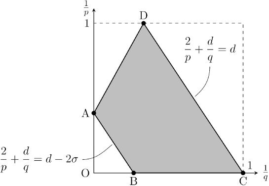
Fig 1. The convex hull $ABCD$ in $(\frac{1}{q},\frac{1}{p})$ plane, where $A,B,C,D$ is the intersection of the boundary of $[0,1]\times[0,1]$ and the two line $\frac{2}{p}+\frac{d}{q}=d$ and $\frac{2}{p}+\frac{d}{q}=d-2\sigma$

For the singular value randomization, we have:

Theorem 1.6.

Let $d\geq 1$ and $0\leq\sigma<\frac{d}{2}$. Let $p,q\in[1,\infty)$ satisfy $\frac{2}{p}+\frac{d}{q}=d-\sigma$ and $(\frac{1}{q},\frac{1}{p})\in ABCD$. Let $\alpha=\min(p,q,2)$ and $r\in[\max(p,q),\infty)$. Then for any $\gamma_{0}\in\mathcal{H}^{\sigma,\alpha}$, it holds that

$$\|\langle\nabla\rangle^{\sigma}\rho(U(t)_{\star}\gamma_{0}^{\omega;\sigma})\|_{L^{r}_{\omega}(\Omega;L^{p}_{t}(\mathbb{R};L^{q}_{x}))}\lesssim r^{\frac{1}{2}}\|\gamma_{0}\|_{\mathcal{H}^{\sigma,\alpha}}.$$ (1.22)

By using full randomization, we can control bigger exponents:

Theorem 1.7.

Let $d\geq 1$ and $0\leq\sigma<\frac{d}{2}$. Let $p\in[2,\infty)$ and $q\in[1,\infty)$ satisfy $\frac{2}{p}+\frac{d}{q}=d$, $\widehat{q}\in[\max(q,2),\infty)$ and $r\in[\max(p,\widehat{q}),\infty)$. Then for any $\gamma_{0}\in\mathcal{H}^{\sigma}$, it holds that

$$\|\langle\nabla\rangle^{\sigma}\rho(U(t)_{\star}\gamma_{0}^{\omega,\widetilde{\omega};\sigma})\|_{L^{r}_{\omega,{\widetilde{\omega}}}(\Omega\times\widetilde{\Omega};L_{t}^{p}(\mathbb{R};L_{x}^{\widehat{q}}))}\lesssim r^{\frac{3}{2}}\|\gamma_{0}\|_{\mathcal{H}^{\sigma}}.$$ (1.23)

Remark 1.8.

On the one hand, by Theorem 1.6, we have

$$\|\rho(U(t)_{\star}\gamma_{0}^{\omega})\|_{L^{p}_{t}(\mathbb{R};L^{q}_{x})}<\infty\text{ for almost all }\omega\in\Omega$$ (1.24)

for any $\gamma_{0}\in\mathfrak{S}^{\min(p,q)}$. On the other hand, by Theorem 1.1, we have

$$\|\rho(U(t)_{\star}\gamma_{0}^{\omega})\|_{L^{p}_{t}(\mathbb{R};L^{q}_{x})}\lesssim\|\gamma_{0}^{\omega}\|_{\mathfrak{S}^{\beta}},$$ (1.25)

where $\beta:=2q/(q+1)$. It is easy to check that $\min(p,q)>\beta$ always holds for all $p,q$ satisfying the assumptions in Theorem 1.1. In this sense, Theorem 1.6 enables us to define the density function $\rho(U(t)_{\star}\gamma_{0})$ with $\gamma_{0}\in\mathfrak{S}^{\alpha}$, where $\alpha$ is bigger than the sharp exponent of the deterministic Strichartz estimates. We can say the same thing about Theorem 1.7.

Remark 1.9.

The optimality of the Schatten exponents $\alpha$ in Theorems 1.6 and 1.7 is a future problem.

Remark 1.10.

The proofs of Theorems 1.6 and 1.7 are quite easy and simple. However, to our best knowledge, these theorems are the first results dealing with this kind of randomization. We should emphasize that the orthogonality of eigenfunctions of $\gamma_{0}$ is not essential in the proofs. In fact, we can prove

$$\left\|\sum_{n=1}^{\infty}a_{n}g_{n}(\omega)|U(t)f_{n}|^{2}\right\|_{L^{r}_{\omega}L^{p}_{t}L^{q}_{x}}\lesssim r^{\frac{1}{2}}\|a\|_{\ell^{\alpha}},$$ (1.26)

$$\left\|\sum_{n=1}^{\infty}a_{n}g_{n}(\omega)|U(t)f_{n}^{\widetilde{\omega}}|^{2}\right\|_{L^{r}_{\omega,{\widetilde{\omega}}}L^{p}_{t}L^{q}_{x}}\lesssim r^{\frac{3}{2}}\|a\|_{\ell^{2}},$$ (1.27)

under the same assumptions for exponents as in Theorems 1.6 and 1.7 without orthogonality of $(f_{n})_{n=1}^{\infty}$. This is because randomization works like orthogonality. (See Lemma 2.2.)

1.5.2. Applications to the Hartree equation for infinitely many particles

First, we give some applications to the local well-posedness of the Cauchy problem ($f$-NLH).

Corollary 1.11 (One-dimensional case).

Let $d=1$. Assume that $w$ is a finite signed Borel measure on $\mathbb{R}$, $f\in L^{1}_{\xi}\cap L^{\infty}_{\xi}$, and $Q_{0}\in\mathfrak{S}^{2}$ is self-adjoint. Then for almost all $\omega\in\Omega$, there exist $T>0$ and a unique solution $Q(t)\in C(0,T;\mathfrak{S}^{2})$ to

$$\left\{\,\begin{aligned} &i\partial_{t}Q=[-\Delta+w\ast\rho_{Q},Q+\gamma_{f}]\\ &Q(0)=Q_{0}^{\omega}\end{aligned}\right.$$ (1.28)

such that $\rho_{Q}\in L^{4}_{t}(0,T;L^{2}_{x})$.

Corollary 1.12 (Two-dimensional case).

Let $d=2$. Let $w\in L^{1}_{x}\cap L^{1+}_{x}$, $f\in L^{1}_{\xi}\cap L^{\infty}_{\xi}$, and $Q_{0}$ be self-adjoint. Assume that $Q_{0}\in\mathfrak{S}^{2-}$ or $Q_{0}\in\mathcal{H}^{0+}$ hold. Then for almost all $\omega\in\Omega$, there exist $T>0$ and a unique solution $Q(t)\in C(0,T;\mathfrak{S}^{2})$ to (1.28) such that $\rho_{Q}\in L^{2}_{t}(0,T;L^{2}_{x})$.

Remark 1.13.

In the above statement, $w\in L^{1+}_{x}$ means there exist $\varepsilon>0$ such that $w\in L^{1+\varepsilon}_{x}$. Similarly, $Q_{0}\in\mathfrak{S}^{2-}$ means there exists $\varepsilon>0$ such that $Q_{0}\in\mathfrak{S}^{2-\varepsilon}$, and $Q_{0}\in\mathcal{H}^{0+}$ means there exists $\varepsilon>0$ such that $Q_{0}\in\mathcal{H}^{\varepsilon}$.

Corollary 1.14 (Three-dimensional case).

Let $d=3$. Let $w\in L^{1}_{x}\cap L^{\infty}_{x}$, $f\in L^{1}_{\xi}\cap L^{\infty}_{\xi}$, and $Q_{0}$ is self-adjoint. Assume that $Q_{0}\in\mathfrak{S}^{3/2-}$ or $Q_{0}\in\mathcal{H}^{0+,3/2}$. Then for almost all $\omega\in\Omega$, there exist $T>0$ and a unique solution $Q(t)\in C(0,T;\mathfrak{S}^{2})$ to (1.28) such that $w\ast\rho_{Q}\in L^{2}_{t}(0,T;L^{2}_{x}\cap L^{\infty}_{x})$.

Remark 1.15.

Our results only claim the unique existence of local solutions; however, we cannot construct any solution in our setting if we only use Theorem 1.1. We emphasize that our result allows strictly bigger Schatten exponents than Theorem 1.1.

	$d=1$	$d=2$	$d=3$
The Schatten exponents that allowed by deterministic Strichartz estimates	$\alpha<2$	$\alpha<\frac{3}{2}$	$\alpha<\frac{4}{3}$
The Schatten exponents that our results allows	$\alpha=2$	$\alpha<2$	$\alpha<\frac{3}{2}$

Remark 1.16.

To show Corollaries 1.11, 1.12, and 1.14, we prove Lemmas 3.1, 3.2, and 3.3. These lemmas are similar to [22, Theorems 5, 6], but they have some advantages. (See Remark 3.4)

In Corollary 1.12, we need $\varepsilon>0$ regularity for initial data $Q_{0}\in\mathfrak{S}^{2}$. However, by using full randomization, we can deal with all Hilbert–Schmidt initial data without any extra regularities:

Corollary 1.17.

Let $d=2$, $f\in L^{1}_{\xi}\cap L^{\infty}_{\xi}$, $w\in L^{1}_{x}\cap L^{\infty}_{x}$, and $Q_{0}\in\mathfrak{S}^{2}$ be self-adjoint. Then for almost all $(\omega,{\widetilde{\omega}})\in\Omega\times\widetilde{\Omega}$, there exists $T>0$ and unique solution $Q(t)\in C(0,T;\mathfrak{S}^{2})$ to

$$\left\{\,\begin{aligned} &i\partial_{t}Q=[-\Delta+w\ast\rho_{Q},Q+\gamma_{f}]\\ &Q(0)=Q_{0}^{\omega,{\widetilde{\omega}}}\end{aligned}\right.$$ (1.29)

such that $w\ast\rho_{Q}\in L^{4}_{t}(0,T;L^{2}_{x}\cap L^{\infty}_{x})$.

Remark 1.18.

Corollary 1.17 immediately follows from Theorem 1.7 and [22, Theorems 5].

Next, we give some application to the scattering problem of the linearized equation of ($f$-NLH):

$$\left\{\,\begin{aligned} &i\partial_{t}Q=[-\Delta,Q]+[w\ast\rho_{Q},\gamma_{f}],\quad Q:\mathbb{R}\to\mathcal{B}(L^{2}_{x}),\\ &Q(0)=Q_{0}.\end{aligned}\right.$$ (1.30)

For given $f$ and $w$, we define a linear operator $\mathcal{L}_{1}=\mathcal{L}_{1}(f,w)$ by

$$\mathcal{L}_{1}[g](t):=\rho\left(i\int_{0}^{t}U(t-\tau)_{\star}[w\ast g(\tau),\gamma_{f}]d\tau\right).$$ (1.31)

Corollary 1.19.

Let $d\geq 2$ and $\sigma=\frac{d}{2}-1$. Let $\langle\xi\rangle^{2\sigma}f(\xi)\in L^{1}_{\xi}\cap L^{\infty}_{\xi}$ and $w$ be a finite signed Borel measure on $\mathbb{R}^{d}$. Assume that $Q_{0}\in\mathcal{H}^{\sigma}$ is self-adjoint, and that $(1+\mathcal{L}_{1}(f,w))^{-1}\in\mathcal{B}(L^{2}_{t}(\mathbb{R};L^{2}_{x}))$. Then for almost all $\omega\in\Omega$, there exists a unique global solution $Q(t)\in C(\mathbb{R};\mathcal{H}^{\sigma})$ to

$$\left\{\,\begin{aligned} &i\partial_{t}Q=[-\Delta,Q]+[w\ast\rho_{Q},\gamma_{f}],\\ &Q(0)=Q_{0}^{\omega;\sigma}\end{aligned}\right.$$ (1.32)

such that $\rho_{Q}\in L^{2}_{t}(\mathbb{R};H^{\sigma}_{x})$. Moreover, $Q(t)$ scatters; that is, there exists $Q_{\pm}\in\mathfrak{S}^{\frac{2d}{d-1}}$ such that

$$U(-t)Q(t)U(t)\to Q_{\pm}\mbox{ in }\mathfrak{S}^{\frac{2d}{d-1}}\mbox{ as }t\to\pm\infty.$$ (1.33)

Remark 1.20.

Some sufficient conditions for $(1+\mathcal{L}_{1})^{-1}\in\mathcal{B}(L^{2}_{t,x})$ are known. For example, see [23, Corollary 1] and Propositions 1.5, 1.6 in [19, Propositions 1.5 and 1.6].

In Corollary 1.19, we need $\sigma=\frac{d}{2}-1$ regularity for initial data. However, we can omit this extra regularity by using full randomization:

Corollary 1.21.

Let $d\geq 2$ and $\sigma:=\frac{d}{2}-1$. Let $\langle\xi\rangle^{\sigma}f(\xi)\in L^{1}_{\xi}\cap L^{\infty}_{\xi}$ and $w$ be a finite signed Borel measure on $\mathbb{R}^{d}$. Assume that $Q_{0}\in\mathfrak{S}^{2}$ and $(1+\mathcal{L}_{1}(f,w))^{-1}\in\mathcal{B}(L^{2}_{t}(\mathbb{R};L^{2}_{x}))$. Then for almost all $(\omega,{\widetilde{\omega}})\in\Omega\times\widetilde{\Omega}$, there exists a unique global solution $Q(t)\in C(\mathbb{R};\mathfrak{S}^{2})$ to

$$\left\{\,\begin{aligned} &i\partial_{t}Q=[-\Delta,Q]+[w\ast\rho_{Q},\gamma_{f}],\\ &Q(0)=Q_{0}^{\omega,{\widetilde{\omega}}}\end{aligned}\right.$$ (1.34)

such that $\rho_{Q}\in L^{2}_{t}(\mathbb{R};L^{2}_{x})$. Moreover, $Q(t)$ scatters; that is, there exists $Q_{\pm}\in\mathfrak{S}^{\frac{2d}{d-1}}$ such that

$$U(-t)Q(t)U(t)\to Q_{\pm}\mbox{ in }\mathfrak{S}^{\frac{2d}{d-1}}\mbox{ as }t\to\pm\infty.$$ (1.35)

Remark 1.22.

Applications of singular value or full randomization to the scattering problems of ($f$-NLH) is an interesting future problem.

2. Probabilistic Strichartz estimates

In this section, we prove the main estimates in this paper.

2.1. Basic tools

In this subsection, we collect some necessary tools.

Lemma 2.1 ([24]; Unit-scale Bernstein inequality).

For all $1\leq r_{1}\leq r_{2}\leq\infty$ and for all $k\in\mathbb{Z}^{d}$, it holds that

$$\|\Pi_{k}f\|_{L^{r_{2}}(\mathbb{R}^{d})}\leq C(r_{1},r_{2})\|\Pi_{k}f\|_{L^{r_{1}}(\mathbb{R}^{d})},$$ (2.1)

where $C(r_{1},r_{2})$ is a constant independent of $k\in\mathbb{Z}^{d}$.

Lemma 2.2 ([9]; Large deviation estimate).

Let $(g_{n})_{n=1}^{\infty}$ be a sequence of random variables introduced in subsection 1.3. Then there is a constant $C>0$ such that

$$\left\|{\sum_{n=1}^{\infty}a_{n}g_{n}}\right\|_{L^{r}_{\omega}(\Omega)}\leq Cr^{\frac{1}{2}}\|a_{n}\|_{\ell^{2}_{n}}.$$ (2.2)

holds for any $r\in[2,\infty)$ and $(a_{n})_{n}\in\ell^{2}_{n}$.

Lemma 2.3.

Let $d\geq 1$. Let $(p,q)\in[2,\infty)^{2}$ be an admissible pair of the standard Strichartz estimates. Let $\widehat{q}\in[q,\infty)$ and $r\in[\max(p,\widehat{q}),\infty)$. For any $f\in L^{2}(\mathbb{R}^{d})$, we have

$$\|U(t)f^{\widetilde{\omega}}\|_{L^{r}_{\widetilde{\omega}}(\widetilde{\Omega};L_{t}^{p}L_{x}^{\widehat{q}}(\mathbb{R}\times\mathbb{R}^{d}))}\lesssim r^{\frac{1}{2}}\|f\|_{L_{x}^{2}(\mathbb{R}^{d})}.$$ (2.3)

Proof.

By Minkowski inequality and Lemma 2.2

$$\|U(t)f^{\widetilde{\omega}}\|_{L^{r}_{\widetilde{\omega}}(\widetilde{\Omega};L_{t}^{p}L_{x}^{\widehat{q}})} \leq\Biggl{\|}\biggl{\|}\sum_{k\in\mathbb{Z}^{d}}U(t)\ell_{k}({\widetilde{\omega}})\Pi_{k}f\biggr{\|}_{L^{r}_{\widetilde{\omega}}(\widetilde{\Omega})}\Biggr{\|}_{L_{t}^{p}L_{x}^{\widehat{q}}}$$ (2.4)

$$\lesssim r^{\frac{1}{2}}\left\|\|U(t)\Pi_{k}f\|_{\ell^{2}_{k}}\right\|_{L_{t}^{p}L_{x}^{\widehat{q}}}.$$ (2.5)

Combining Minkowski inequality, Lemma 2.1 and Strichartz estimate, we have

$$\|U(t)f^{\widetilde{\omega}}\|_{L^{r}_{{\widetilde{\omega}}}(\widetilde{\Omega};L_{t}^{p}L_{x}^{\hat{q}})}\lesssim r^{\frac{1}{2}}\left\|\|U(t)\Pi_{k}f\|_{L_{t}^{p}L_{x}^{\widehat{q}}}\right\|_{\ell^{2}_{k}}$$ (2.6)

$$\lesssim r^{\frac{1}{2}}\left\|\|U(t)\Pi_{k}f\|_{L_{t}^{p}L_{x}^{q}}\right\|_{\ell^{2}_{k}}\lesssim r^{\frac{1}{2}}\left(\sum_{k\in\mathbb{Z}^{d}}\|\Pi_{k}f\|_{L_{x}^{2}}^{2}\right)^{1/2}=r^{\frac{1}{2}}\|f\|_{L_{x}^{2}},$$ (2.7)

which concludes the desired estimate. ∎

2.2. Proof of Theorem 1.6

We write the singular value decomposition of $\langle\nabla\rangle^{\sigma}_{\star}\gamma_{0}$ as $\langle\nabla\rangle^{\sigma}_{\star}\gamma_{0}=\sum_{n}a_{n}|u_{n}\rangle\langle v_{n}|$. Then we have

$$\gamma_{0}^{\omega;\sigma} =\sum_{n=1}^{\infty}a_{n}g_{n}(\omega)|\langle\nabla\rangle^{-\sigma}u_{n}\rangle\langle\langle\nabla\rangle^{-\sigma}v_{n}|=\sum_{n=1}^{\infty}a_{n}g_{n}(\omega)|\widetilde{u_{n}}\rangle\langle\widetilde{v_{n}}|$$ (2.8)

By Minkowski inequality and Lemma 2.2, we have

$$\|\langle\nabla\rangle^{\sigma}\rho(U(t)_{\star}\gamma_{0}^{\omega;\sigma})\|_{L^{r}_{\omega}(\Omega;L_{t}^{p}L_{x}^{q})}$$

$$\quad=\left\|{\sum_{n=1}^{\infty}a_{n}g_{n}(\omega)\langle\nabla\rangle^{\sigma}\left(\overline{U(t)\widetilde{v_{n}}}U(t)\widetilde{u_{n}}\right)}\right\|_{L^{r}_{\omega}(\Omega;L_{t}^{p}L_{x}^{q})}$$

$$\quad\leq\left\|{\left\|\sum_{n=1}^{\infty}a_{n}g_{n}(\omega)\langle\nabla\rangle^{\sigma}\left(\overline{U(t)\widetilde{v_{n}}}U(t)\widetilde{u_{n}}\right)\right\|_{L^{r}_{\omega}(\Omega)}}\right\|_{L_{t}^{p}L_{x}^{q}}$$

$$\quad\lesssim r^{\frac{1}{2}}\left\|{\left\|{a_{n}\langle\nabla\rangle^{\sigma}\left(\overline{U(t)\widetilde{v_{n}}}U(t)\widetilde{u_{n}}\right)}\right\|_{\ell_{n}^{2}}}\right\|_{L_{t}^{p}L_{x}^{q}}.$$

Since $(\frac{1}{q},\frac{1}{p})\in ABCD$, there exists $p_{0},q_{0},p_{1},q_{1}\in[1,\infty]$ such that

$$\frac{2}{p_{0}}+\frac{d}{q_{0}}=d,\quad\frac{2}{p_{1}}+\frac{d}{q_{1}}=d-2\sigma.$$ (2.9)

Using $\ell^{\alpha}\subset\ell^{2}$, Minkowski inequality, Strichartz estimate, and fractional Leibniz rule, we obtain

$$\left\|{\left\|{a_{n}\langle\nabla\rangle^{\sigma}\left(\overline{U(t)\widetilde{v_{n}}}U(t)\widetilde{u_{n}}\right)}\right\|_{\ell_{n}^{2}}}\right\|_{L_{t}^{p}L_{x}^{q}} \leq\left\|{\left\|{a_{n}\langle\nabla\rangle^{\sigma}\left(\overline{U(t)\widetilde{v_{n}}}U(t)\widetilde{u_{n}}\right)}\right\|_{\ell_{n}^{\alpha}}}\right\|_{L_{t}^{p}L_{x}^{q}}$$ (2.10)

$$\leq\left\|{\left\|{a_{n}\langle\nabla\rangle^{\sigma}\left(\overline{U(t)\widetilde{v_{n}}}U(t)\widetilde{u_{n}}\right)}\right\|_{L_{t}^{p}L_{x}^{q}}}\right\|_{\ell_{n}^{\alpha}}$$ (2.11)

$$\lesssim\left\|a_{n}\|U(t)\widetilde{u_{n}}\|_{L_{t}^{2p_{0}}L_{x}^{2q_{0}}}\|U(t)\widetilde{v_{n}}\|_{L_{t}^{2p_{1}}H_{x}^{\sigma,2q_{1}}}\right\|_{\ell^{\alpha}_{n}}$$ (2.12)

$$\quad+\left\|a_{n}\|U(t)\widetilde{u_{n}}\|_{L_{t}^{2p_{1}}H_{x}^{\sigma,2q_{1}}}^{\alpha}\|U(t)\widetilde{v_{n}}\|_{L_{t}^{2p_{0}}L_{x}^{2q_{0}}}^{\alpha}\right\|_{\ell^{\alpha}_{n}}$$ (2.13)

$$\lesssim\|a\|_{\ell^{\alpha}}=\|\gamma_{0}\|_{\mathcal{H}^{\sigma,\alpha}}.$$ (2.14)

∎

2.3. Proof of Theorem 1.7

We write the singular value decomposition of $\gamma_{0}$ as $\langle\nabla\rangle^{\sigma}_{\star}\gamma_{0}=\sum_{n}a_{n}|u_{n}\rangle\langle v_{n}|$. Then we have

$$\gamma_{0}^{\omega,{\widetilde{\omega}};\sigma} =\sum_{n=1}^{\infty}a_{n}g_{n}(\omega)|\langle\nabla\rangle^{-\sigma}u_{n}^{\widetilde{\omega}}\rangle\langle\langle\nabla\rangle^{-\sigma}v_{n}^{\widetilde{\omega}}|=\sum_{n=1}^{\infty}a_{n}g_{n}(\omega)|\widetilde{u_{n}}^{\widetilde{\omega}}\rangle\langle\widetilde{v_{n}}^{\widetilde{\omega}}|$$ (2.15)

By Minkowski’s inequality, Lemmas 2.2 and 2.3, we have

$$\|\langle\nabla\rangle^{\sigma}\rho(U(t)_{\star}\gamma_{0}^{\omega,\widetilde{\omega}})\|_{L^{r}_{\omega,{\widetilde{\omega}}}(\Omega\times\widetilde{\Omega};L_{t}^{p}L_{x}^{\widehat{q}})}$$ (2.16)

$$\quad=\left\|\sum_{n=1}^{\infty}a_{n}g_{n}(\omega)\langle\nabla\rangle^{\sigma}\left(\overline{U(t)\widetilde{v_{n}}^{\widetilde{\omega}}}U(t)\widetilde{u_{n}}^{\widetilde{\omega}}\right)\right\|_{L^{r}_{\omega,{\widetilde{\omega}}}L^{p}_{t}L^{\widehat{q}}_{x}}$$ (2.17)

$$\quad\lesssim r^{\frac{1}{2}}\left\|a_{n}\langle\nabla\rangle^{\sigma}\left(\overline{U(t)\widetilde{v_{n}}^{\widetilde{\omega}}}U(t)\widetilde{u_{n}}^{\widetilde{\omega}}\right)\right\|_{L^{r}_{\widetilde{\omega}}L^{p}_{t}L^{\widehat{q}}_{x}\ell_{n}^{2}}$$ (2.18)

$$\quad\leq r^{\frac{1}{2}}\left\|a_{n}\langle\nabla\rangle^{\sigma}\left(\overline{U(t)\widetilde{v_{n}}^{\widetilde{\omega}}}U(t)\widetilde{u_{n}}^{\widetilde{\omega}}\right)\right\|_{\ell_{n}^{2}L^{r}_{\widetilde{\omega}}L^{p}_{t}L^{\widehat{q}}_{x}}$$ (2.19)

$$\quad\lesssim r^{\frac{1}{2}}\left\|a_{n}\|U(t)u_{n}^{\widetilde{\omega}}\|_{L^{2r}_{\widetilde{\omega}}L^{2p}_{t}L^{2{\widehat{q}}}_{x}}\|U(t)v_{n}^{\widetilde{\omega}}\|_{L^{2r}_{\widetilde{\omega}}L^{2p}_{t}L^{2{\widehat{q}}}_{x}}\right\|_{\ell_{n}^{2}}\lesssim r^{\frac{3}{2}}\|\gamma_{0}\|_{\mathfrak{S}^{2}}.$$ (2.20)

∎

2.4. No gain of regularities by the randomizations

We can obtain neither lower Schatten integrabilities nor higher Sobolev regularities by the singular value randomization unless $(g_{n})_{n=1}^{\infty}$ doesn’t gather to 0. This argument is similar to [9, Lemma B.1].

Proposition 2.4.

Assume that the sequence of random variables $(g_{n})_{n=1}^{\infty}$ introduced in subsection 1.3 satisfies the following condition: there exists $C>0$ such that

$$\limsup_{n\to\infty}\mathbb{P}(\{\omega\in\Omega:|g_{n}(\omega)|\leq C\})<1.$$ (2.21)

Let $1<\beta<\alpha<\infty$ and $\sigma\in\mathbb{R}$. Then $\langle\nabla\rangle^{\sigma}_{\star}\gamma_{0}\in\mathfrak{S}^{\alpha}\setminus\mathfrak{S}^{\beta}$ implies $\langle\nabla\rangle^{\sigma}_{\star}\gamma_{0}^{\omega;\sigma}\in\mathfrak{S}^{\alpha}\setminus\mathfrak{S}^{\beta}$ for almost all $\omega\in\Omega$.

Remark 2.5.

If $(g_{n})_{n=1}^{\infty}$ is a sequence of Gaussian random variables with uniformly lower bounded variances, (2.1) is satisfied.

Proof.

We can assume that $\sigma=0$. First, we prove $\gamma_{0}^{\omega}\in\mathfrak{S}^{\alpha}$ for almost all $\omega\in\Omega$. We have by (1.12)

$$\mathbb{E}\left[\sum_{n=1}^{\infty}|a_{n}g_{n}(\omega)|^{\alpha}\right]=\sum_{n=1}^{\infty}|a_{n}|^{\alpha}\mathbb{E}[|g_{n}|^{\alpha}]\lesssim\|a\|_{\ell^{\alpha}}<\infty.$$ (2.22)

Therefore, we obtain

$$\sum_{n=1}^{\infty}|a_{n}g_{n}(\omega)|^{\alpha}<\infty$$ (2.23)

for almost all $\omega\in\Omega$.

Next, we prove $\gamma_{0}^{\omega}\notin\mathfrak{S}^{\beta}$ for almost all $\omega\in\Omega$. From the assumption (2.21), there exists $\delta\in(0,1)$ and $N\in\mathbb{N}$ such that $\mu_{n}([-c,c])\leq 1-\delta$ holds for any $n\geq N$.

$$\int_{\Omega}e^{-\|\gamma_{0}^{\omega}\|_{\mathfrak{S}^{\beta}}^{\beta}}\,d\mathbb{P}(\omega)=\int_{\Omega}e^{-\sum_{n=1}^{\infty}|a_{n}g_{n}(\omega)|^{\beta}}\,d\mathbb{P}(\omega)$$ (2.24)

$$=\prod_{n=1}^{\infty}\left(\int_{\{|x|\leq c\}}e^{-|a_{n}x|^{\beta}}\,d\mu_{n}(x)+\int_{\{|x|>c\}}e^{-|a_{n}x|^{\beta}}\,d\mu_{n}(x)\right)$$ (2.25)

$$\leq\prod_{n=N}^{\infty}\left(\mu_{n}([-c,c])(1-e^{-|a_{n}c|^{\beta}})+e^{-|a_{n}c|^{\beta}}\right)$$ (2.26)

$$\leq\prod_{n=N}^{\infty}\left((1-\delta)+e^{-|a_{n}c|^{\beta}}\delta\right)=\prod_{n=N}^{\infty}\left(1-\delta(1-e^{-|a_{n}c|^{\beta}})\right).$$ (2.27)

Since $|a_{n}c|^{\beta}\to+0$ from $\gamma_{0}\in\mathfrak{S}^{\alpha}$, there exists $\lambda\in(0,1)$ such that

$$1-e^{-|a_{n}c|^{\beta}}\geq\lambda|a_{n}c|^{\beta}$$ (2.28)

for all $n\in\mathbb{N}$. Combining $\|\gamma_{0}\|_{\mathfrak{S}^{\beta}}=\infty$,

$$\sum_{n=N}^{\infty}(1-e^{-|a_{n}c|^{\beta}})\geq\lambda c^{\beta}\sum_{n=N}^{\infty}|a_{n}|^{\beta}=\infty.$$ (2.29)

Therefore, we obtain that

$$\int_{\Omega}e^{-\|\gamma_{0}^{\omega}\|_{\mathfrak{S}^{\beta}}^{\beta}}\,d\mathbb{P}(\omega) \leq\prod_{n=N}^{\infty}\left(1-\delta(1-e^{-|a_{n}c|^{\beta}})\right)$$ (2.30)

$$\leq\exp{\biggl{(}-\delta\sum_{n=N}^{\infty}(1-e^{-|a_{n}c|^{\beta}})\biggr{)}}=0,$$ (2.31)

which concludes that $\|\gamma_{0}^{\omega}\|_{\mathfrak{S}^{\beta}}=\infty$ almost surely. ∎

We also cannot gain any regularities by the full randomization. Before proving it, we prepare a lemma:

Lemma 2.6.

Let $d\geq 1$ and $\alpha\in[1,\infty]$. Let $f:\mathbb{R}^{d}\to\mathbb{C}$ be a measurable function. Let $A\in\mathfrak{S}^{\alpha}$ be self-adjoint and $f(x)Af(x)\neq 0$, where $f(x)$ is the standard multiplication operator. Define $\operatorname{supp}A$ by

$$\operatorname{supp}A:=\bigcup_{u\in\mathrm{Ran}A}\operatorname{supp}u.$$ (2.32)

Assume that

$$a\leq|f(x)|\leq b\text{ for almost all }x\in\operatorname{supp}A.$$ (2.33)

Then it holds that

$$a^{2}\|A\|_{\mathfrak{S}^{\alpha}}\leq\|f(x)Af(x)\|_{\mathfrak{S}^{\alpha}}\leq b^{2}\|A\|_{\mathfrak{S}^{\alpha}}$$ (2.34)

Proof.

We can assume $a>0$. For the first inequality, we have

$$a^{2}\|A\|_{\mathfrak{S}^{\alpha}}=\left\|\frac{a}{f(x)}\mathbbm{1}_{\operatorname{supp}A}(x)f(x)Af(x)\mathbbm{1}_{\operatorname{supp}A}(x)\frac{a}{f(x)}\right\|_{\mathfrak{S}^{\alpha}}\leq\|f(x)Af(x)\|_{\mathfrak{S}^{\alpha}}.$$ (2.35)

For the second inequality, we have

$$\|f(x)Af(x)\|_{\mathfrak{S}^{\alpha}}\leq\|f(x)\mathbbm{1}_{\operatorname{supp}A}(x)\|_{\mathcal{B}(L^{2}_{x})}^{2}\|A\|_{\mathfrak{S}^{\alpha}}\leq b^{2}\|A\|_{\mathfrak{S}^{\alpha}}.$$ (2.36)

∎

Proposition 2.7.

Let $1<\beta<\alpha<\infty$ and $\sigma\in\mathbb{R}$. Assume that

$$\left|{\left\{\xi\in\mathbb{R}^{d}\mid\sum_{k\in\mathbb{Z}^{d}}\ell_{k}(\widetilde{\omega})\chi_{k}(\xi)=0\right\}}\right|=0,\quad\mbox{ almost all }\widetilde{\omega}\in\widetilde{\Omega}.$$ (2.37)

Then if $\langle\nabla\rangle^{\sigma}_{\star}\gamma_{0}\in\mathfrak{S}^{\alpha}\setminus\mathfrak{S}^{\beta}$ and $\gamma_{0}$ is self-adjoint, it holds that $\langle\nabla\rangle^{\sigma}_{\star}\gamma_{0}^{\omega,{\widetilde{\omega}};\sigma}\in\mathfrak{S}^{\alpha}\setminus\mathfrak{S}^{\beta}$ for almost all $(\omega,{\widetilde{\omega}})\in\Omega\times\widetilde{\Omega}$.

Remark 2.8.

If $(\ell_{k})_{k\in\mathbb{Z}^{d}}$ is a sequence of Gaussian random variables, (2.2) is satisfied, since $\ell_{k}(\widetilde{\omega})\xi_{k}(\xi)$ is $0$ except for finite $k\in\mathbb{Z}^{d}$ for each $\xi\in\mathbb{R}^{d}$.

Proof.

We can assume that $\sigma=0$. By (2.37), there exists $\mathcal{R}^{-1}_{\widetilde{\omega}}$ for almost all ${\widetilde{\omega}}\in\widetilde{\Omega}$. We write

$$\mathcal{R}_{\widetilde{\omega}}=\mathcal{F}^{-1}_{\xi\to x}R_{\widetilde{\omega}}(\xi)\mathcal{F}_{x\to\xi},\quad\mathcal{R}_{\widetilde{\omega}}^{-1}=\mathcal{F}^{-1}_{\xi\to x}R_{\widetilde{\omega}}(\xi)^{-1}\mathcal{F}_{x\to\xi}.$$ (2.38)

Define

$$P_{\delta}:=\mathcal{F}^{-1}_{\xi\to x}\mathbbm{1}_{\{|\mathcal{R}_{\widetilde{\omega}}(\xi)|\leq A\}}\mathcal{F}_{x\to\xi},\quad P_{A}^{\perp}:=\mathcal{F}^{-1}_{\xi\to x}\mathbbm{1}_{\{|\mathcal{R}_{\widetilde{\omega}}(\xi)|>A\}}\mathcal{F}_{x\to\xi}$$ (2.39)

First, we prove $\gamma_{1}:=\mathcal{R}_{\widetilde{\omega}}\gamma_{0}\mathcal{R}_{\widetilde{\omega}}\in\mathfrak{S}^{\alpha}$. By Lemma 2.6 and $\gamma_{0}\neq 0$, we have

$$\infty>\|\gamma_{0}\|_{\mathfrak{S}^{\alpha}}\geq\|P_{A}\mathcal{R}_{\widetilde{\omega}}^{-1}\gamma_{1}\mathcal{R}_{\widetilde{\omega}}^{-1}P_{A}\|_{\mathfrak{S}^{\alpha}} \geq A^{-2}\|\gamma_{1}\|_{\mathfrak{S}^{\alpha}}$$ (2.40)

for sufficiently large $A>0$. Next, we prove $\gamma_{1}\notin\mathfrak{S}^{\beta}$. By (2.37), we have $\gamma_{1}\neq 0$ for almost all ${\widetilde{\omega}}\in\widetilde{\Omega}$. Then for sufficiently small $A>0$, we have by Lemma 2.6 that

$$\|\gamma_{1}\|_{\mathfrak{S}^{\beta}}\geq\|P_{A}^{\perp}\mathcal{R}_{\widetilde{\omega}}\gamma_{0}\mathcal{R}_{\widetilde{\omega}}P_{A}^{\perp}\|_{\mathfrak{S}^{\beta}}\geq A^{2}\|\gamma_{0}\|_{\mathfrak{S}^{\beta}}=\infty.$$ (2.41)

∎

3. Application to the Hartree equation: Local well-posedness theory

In this section, we prove Corollaries 1.11, 1.12, and 1.14. By Theorem 1.6 and 2.4, it suffices to prove the following lemmas:

Lemma 3.1 (One-dimensional case).

Let $d=1$. Let $w$ be a finite signed Borel measure on $\mathbb{R}$, $f\in L^{1}_{\xi}\cap L^{\infty}_{\xi}$, and $Q_{0}$ be self-adjoint. Assume that $Q_{0}\in\mathfrak{S}^{2}$ and $\|\rho(U(t)_{\star}Q_{0})\|_{L^{4}_{t,{\rm loc}}(\mathbb{R};L^{2}_{x})}<\infty$. Then there exist $T>0$ and a unique solution $Q(t)\in C(0,T;\mathfrak{S}^{2})$ to ($f$-NLH) such that $\rho_{Q}\in L^{4}_{t}(0,T;L^{2}_{x})$.

Lemma 3.2 (Two-dimensional case).

Let $d=2$. Let $f\in L^{1}_{\xi}\cap L^{\infty}_{\xi}$ and $Q_{0}$ be self-adjoint. Assume that there exists $\varepsilon>0$ such that $w\in L^{1}_{x}\cap L^{1+\varepsilon}_{x}$. Assume that $Q_{0}\in\mathfrak{S}^{2-\varepsilon}$ or $Q_{0}\in\mathcal{H}^{\varepsilon}$ hold, and $\|\rho(U(t)_{\star}Q_{0})\|_{L^{2}_{t,{\rm loc}}(\mathbb{R};L^{2}_{x})}<\infty$. Then there exist $T>0$ and a unique solution $Q(t)\in C(0,T;\mathfrak{S}^{2})$ to ($f$-NLH) such that $\rho_{Q}\in L^{2}_{t}(0,T;L^{2}_{x})$.

Lemma 3.3 (Three-dimensional case).

Let $d=3$. Let $w\in L^{1}_{x}\cap L^{\infty}_{x}$, $f(\xi)\in L^{1}_{\xi}\cap L^{\infty}_{\xi}$, and $Q_{0}$ be self-adjoint. Assume that there exists $\varepsilon>0$ such that $Q_{0}\in\mathfrak{S}^{3/2-\varepsilon}$ or $Q_{0}\in\mathcal{H}^{\varepsilon,3/2}$. Assume that $\|w\ast\rho(U(t)_{\star}Q_{0})\|_{L^{2}_{t,{\rm loc}}(\mathbb{R};L^{2}_{x}\cap L^{\infty}_{x})}<\infty$. Then there exist $T>0$ and a unique solution $Q(t)\in C(0,T;\mathfrak{S}^{2})$ to ($f$-NLH) such that $w\ast\rho_{Q}\in L^{2}_{t}(0,T;L^{2}_{x}\cap L^{\infty}_{x})$.

Remark 3.4.

The above lemmas are similar to [22, Theorems 5, 6]. One of these results never includes the other; hence, there is no simple superiority or inferiority. However, our results have some advantages:

• In [22, Theorem 5], we need $w\in L^{1}_{x}\cap L^{\infty}_{x}$ to get local solution; however, all general finite signed Borel measures are acceptable in Lemma 3.1, and $w\in L^{1}_{x}\cap L^{1+0}_{x}$ is sufficient in Lemma 3.2.

• In [22, Theorem 5], we only get information of the indirect object $w\ast\rho_{Q}$; however, we can have more direct information of $\rho_{Q}$ in Lemmas 3.1 and 3.2.

• In [22, Theorem 6] with $d=3$, we need $\langle\xi\rangle f(\xi)\in L^{2}_{x}$ and $w\in W^{1,1}_{x}\cap W^{1,\infty}_{x}$ and $\langle\nabla\rangle Q_{0}\in\mathfrak{S}^{2}$. However, we do not need this type of regularities for $f$, $w$, and $Q_{0}$ in Lemma 3.3.

3.1. Preliminaries

We collect the necessary tools in this subsection. Let $H$ and $K$ be separable complex Hilbert spaces. For $\alpha\in[1,\infty]$ and compact operator $A:H\to K$, we define Schatten $\alpha$–norm by

$$\|A\|_{\mathfrak{S}^{\alpha}(H\to K)}:=\begin{cases}&\left({\rm Tr}_{H}(|A^{*}A|^{\frac{\alpha}{2}})\right)^{\frac{1}{\alpha}}\mbox{ if }1\leq\alpha<\infty,\\ &\|A\|_{\mathcal{B}(H\to K)}\mbox{ if }\alpha=\infty,\end{cases}$$ (3.1)

where ${\rm Tr}_{H}$ is the trace in $H$ and $\mathcal{B}(H\to K)$ is the space of all bound linear operators from $H$ to $K$. For each $\alpha\in[1,\infty]$, we write

$$\mathfrak{S}^{\alpha}:=\mathfrak{S}^{\alpha}(L^{2}_{x}\to L^{2}_{x}),\quad\mathfrak{S}^{\alpha}_{t,x}:=\mathfrak{S}^{\alpha}(L^{2}_{t,x}\to L^{2}_{t,x}),$$ (3.2)

$$\mathfrak{S}^{\alpha}_{x\to(t,x)}:=\mathfrak{S}^{\alpha}(L^{2}_{x}\to L^{2}_{t,x}),\quad\mathfrak{S}^{\alpha}_{(t,x)\to x}:=\mathfrak{S}^{\alpha}(L^{2}_{t,x}\to L^{2}_{x}).$$ (3.3)

Now, we recall the notations, definitions, and results in [20, Section 3]. Let $I\subset\mathbb{R}$ be an interval. Assume that $A(t)\in\mathcal{B}(L^{2}_{x})$ for all $t\in I$, $\sup_{t\in I}\|A(t)\|_{\mathcal{B}}<\infty$, and $I\ni t\mapsto A(t)\in\mathcal{B}(L^{2}_{x})$ is strongly continuous. Define $A^{\ocircle}:L^{2}_{x}\to C_{t}(I;L^{2}_{x})$ and $A^{\oast}:L^{1}_{t}(I;L^{2}_{x})\to L^{2}_{x}$ by

$$(A^{\ocircle}u_{0})(t,x):=(A(t)u_{0})(x),$$ (3.4)

$$(A^{\oast}g)(x):=\int_{I}A(\tau)^{*}g(\tau,x)d\tau.$$ (3.5)

Note that $A^{\ocircle}$ and $A^{\oast}$ are formally adjoint to each other. The following lemma is useful.

Lemma 3.5 ([18] Lemma 3; Duality principle).

Let $p,q,\alpha\in[1,\infty]$. The following are equivalent:

• For any $\gamma_{0}\in\mathfrak{S}^{\alpha}$,

  $$\|\rho(A(t)_{\star}\gamma_{0})\|_{L^{p}_{t}(I,L^{q}_{x})}\leq C\|\gamma_{0}\|_{\mathfrak{S}^{\alpha}}.$$ (3.6)

• For any $g\in L^{2p^{\prime}}_{t}(I,L^{2q^{\prime}}_{x})$,

  $$\|gA^{\ocircle}\|_{\mathfrak{S}^{2\alpha^{\prime}}_{x\to({t,x})}}\leq C^{\prime}\|g\|_{L^{2p^{\prime}}_{t}(I,L^{2q^{\prime}}_{x})}.$$ (3.7)

• For any $g\in L^{2p^{\prime}}_{t}(I,L^{2q^{\prime}}_{x})$,

  $$\|A^{\oast}g\|_{\mathfrak{S}^{2\alpha^{\prime}}_{({t,x})\to x}}\leq C^{\prime\prime}\|g\|_{L^{2p^{\prime}}_{t}(I,L^{2q^{\prime}}_{x})}.$$ (3.8)

Moreover, $\sqrt{C}$, $C^{\prime}$ and $C^{\prime\prime}$ coincide.

Let $p,q\in[1,\infty]$ and $\alpha\in[1,\infty]$. We call $(p,q,\alpha)$ admissible when $\frac{1}{\alpha}\geq\frac{1}{dp}+\frac{1}{q}$ and $\alpha<p$ hold. The following orthonormal Strichartz estimate is significant:

Theorem 3.6 ([17] Theorem 1; [18] Theorem 8; [2] Theorem 1.5).

Let $d\geq 1$. Let $p,q,\alpha\in(1,\infty)$ and $\sigma\in[0,\frac{d}{2})$. Assume that $(p,q,\alpha)$ is admissible and $\frac{2}{p}+\frac{d}{q}=d-2\sigma$. Then

$$\|\rho(U(t)_{\star}Q_{0})\|_{L^{p}_{t}L^{q}_{x}}\lesssim\|\langle\nabla\rangle^{\sigma}_{\star}Q_{0}\|_{\mathfrak{S}^{\alpha}}$$ (3.9)

holds for any $Q_{0}\in\mathfrak{S}^{\alpha}$.

Lemma 3.7.

Let $2\leq\alpha\leq\infty$. Assume that $\mu,\nu\in[1,\infty]$ satisfy $\sigma(\mu,\nu)=2$ and

• $1\leq\mu\leq\frac{4}{3}$ when $d=1$,

• $1\leq\mu<2$ when $d=2$,

• $1\leq\mu\leq 2$ when $d\geq 3$.

Then we have

$$\left\|\int_{0}^{T}U(\tau)^{*}V(\tau)Q(\tau)U(\tau)d\tau\right\|_{\mathfrak{S}^{\alpha}}\lesssim\|V\|_{L^{\mu}_{t}(0,T;L^{\nu}_{x})}\|Q\|_{C(0,T;\mathfrak{S}^{\alpha})}.$$

Proof.

We assume $d\geq 3$ since we can prove the other cases similarly. It is straightforward to verify the case $\mu=1$. Hence, we assume that $\mu=2$. First, we consider the case $\alpha=2$. Let $\frac{1}{q}:=\frac{1}{2}-\frac{1}{d}$. Then we have by the endpoint Strichartz estimate (see [21])

$$\left|{{\rm Tr}\left[A\int_{0}^{T}U(\tau)^{*}V(\tau)Q(\tau)U(\tau)d\tau\right]}\right| =\left|{\int_{0}^{T}d\tau{\rm Tr}\left[Q(\tau)U(\tau)AU(\tau)^{*}V(\tau)\right]}\right|$$

$$\leq\left\|\rho\left[Q(t)(U(t)_{\star}A)\right]\right\|_{L^{2}_{T}L^{d^{\prime}}_{x}}\|V\|_{L^{2}_{T}L^{d}_{x}}$$

$$\leq\|\rho_{Q^{2}}^{1/2}\|_{C_{T}L^{2}_{x}}\|\rho(U(t)_{\star}|A|^{2})^{\frac{1}{2}}\|_{L^{2}_{T}L^{q}_{x}}\|V\|_{L^{2}_{T}L^{d}_{x}}$$

$$\leq\|Q\|_{C_{T}\mathfrak{S}^{2}}\|A\|_{\mathfrak{S}^{2}}\|V\|_{L^{2}_{T}L^{d}_{x}}.$$

Next, we consider the case $\alpha=\infty$. Let $A\in\mathfrak{S}^{1}$. Then we have

$$\left|{{\rm Tr}\left[A\int_{0}^{T}U(\tau)^{*}V(\tau)Q(\tau)U(\tau)d\tau\right]}\right|$$

$$\quad\leq\left\|\rho\left[Q(t)(U(t)_{\star}A)\right]\right\|_{L^{2}_{T}L^{d^{\prime}}_{x}}\|V\|_{L^{2}_{T}L^{d}_{x}}$$

$$\quad\leq\||\rho(Q(t)U(t)|A|U(t)^{*}Q(t))|^{\frac{1}{2}}\|_{L^{\infty}_{T}L^{2}_{x}}\||\rho(U(t)_{\star}|A|)|^{\frac{1}{2}}\|_{L^{2}_{T}L^{q}_{x}}\|V\|_{L^{2}_{T}L^{d}_{x}}$$

$$\quad\leq\|Q\|_{C_{T}\mathfrak{S}^{\infty}}\|A\|_{\mathfrak{S}^{1}}\|V\|_{L^{2}_{T}L^{d}_{x}}.$$

∎

3.2. Proof of Lemma 3.1

We have the Duhamel form:

$$\left\{\begin{aligned} Q(t)&=\Phi_{1}[Q,\rho_{Q}],\\ \rho_{Q}(t)&=\Phi_{2}[Q,\rho_{Q}],\end{aligned}\right.$$ (3.10)

where

$$\Phi_{1}[Q,\rho_{Q}] :=U(t)_{\star}Q_{0}+\mathcal{D}_{V}[Q]+\mathcal{D}_{V}[\gamma_{f}]$$ (3.11)

$$:=U(t)_{\star}Q_{0}-i\int_{0}^{t}U(t-\tau)_{\star}[V(\tau),Q(\tau)]d\tau-i\int_{0}^{t}U(t-\tau)_{\star}[V(\tau),\gamma_{f}]d\tau,$$ (3.12)

$$V :=w\ast\rho_{Q},$$ (3.13)

and

$$\Phi_{2}[Q,\rho_{Q}](t) :=\rho(U(t)_{\star}Q_{0})+\rho(\mathcal{D}_{V}[U(t)_{\star}Q_{0}])$$ (3.14)

$$\quad+\rho(\mathcal{D}_{V}^{2}[Q])+\rho(\mathcal{D}_{V}^{2}[\gamma_{f}])-\mathcal{L}_{1}(\rho_{Q}).$$ (3.15)

We used the notation $\mathcal{L}_{1}[\rho_{Q}]:=-\rho(\mathcal{D}[\gamma_{f}])$. Define

$$E(T,R):=\{(Q,g)\in C_{T}\mathfrak{S}^{2}\times L^{4}_{T}L^{2}_{x}:\|Q\|_{C_{T}\mathfrak{S}^{2}}\leq R,\|g\|_{L^{4}_{T}L^{2}_{x}}\leq R\},$$ (3.16)

where $R:=2(\|Q_{0}\|_{\mathfrak{S}^{2}}+\|\rho(U(t)_{\star}Q_{0})\|_{L^{4}_{t}L^{2}_{x}})$ and $T>0$ will be chosen later. We prove that $\Phi:E(T,R)\ni(Q,g)\to(\Phi_{1}[Q,g],\Phi_{2}[Q,g])\in E(T,R)$ is a contraction mapping.

Let $(Q,g)\in E(T,R)$. Then by Lemma 3.7 and Kato–Seiler–Simon’s inequality (see [29] and [30, Theorem 4.1]), we have

$$\|\Phi_{1}[Q,g](t)\|_{\mathfrak{S}^{2}} \leq\|Q_{0}\|_{\mathfrak{S}^{2}}+2\left\|\int_{0}^{t}U(\tau)^{*}V(\tau)Q(\tau)U(\tau)d\tau\right\|_{\mathfrak{S}^{2}}$$ (3.17)

$$\quad+2\left\|\int_{0}^{t}U(\tau)^{*}V(\tau)\gamma_{f}(\tau)U(\tau)d\tau\right\|_{\mathfrak{S}^{2}}$$ (3.18)

$$\leq\|Q_{0}\|_{\mathfrak{S}^{2}}+C\|V\|_{L^{4/3}_{T}L^{2}_{x}}\|Q\|_{C_{T}\mathfrak{S}^{2}}+2\int_{0}^{T}\|V(\tau)\gamma_{f}\|_{\mathfrak{S}^{2}}d\tau$$ (3.19)

$$\leq\frac{R}{2}+CT^{\frac{1}{2}}R^{2}+C\|f\|_{L^{2}_{\xi}}T^{\frac{3}{4}}R\leq R,$$ (3.20)

if we choose $T>0$ sufficiently small. For the density function, we have

$$\|\Phi_{2}[Q,g]\|_{L^{4}_{T}L^{2}_{x}} \leq\|\rho(U(t)_{\star}Q_{0})\|_{L^{4}_{T}L^{2}_{x}}+\|\rho(\mathcal{D}_{V}[U(t)_{\star}Q_{0}])\|_{L^{4}_{T}L^{2}_{x}}$$ (3.21)

$$\quad+\|\rho(\mathcal{D}_{V}^{2}[Q])\|_{L^{4}_{T}L^{2}_{x}}+\|\rho(\mathcal{D}_{V}^{2}[\gamma_{f}])\|_{L^{4}_{T}L^{2}_{x}}+\|\mathcal{L}_{1}(\rho_{Q})\|_{L^{4}_{T}L^{2}_{x}}$$ (3.22)

$$=:A_{1}+A_{2}+A_{3}+A_{4}+A_{5}.$$ (3.23)

By definition of $R$, we obtain

$$A_{1}\leq\frac{R}{2}.$$ (3.24)

Let

$$\mathcal{V}:=\int_{0}^{T}U(\tau)^{*}V(\tau)U(\tau)d\tau.$$ (3.25)

Since it follows from Theorem 1.1 and the duality argument that

$$\left\|\rho(U(t)[\mathcal{V},Q_{0}]U(t)^{*})\right\|_{L^{4}_{T}L^{2}_{x}} \lesssim\|\mathcal{V}Q_{0}\|_{\mathfrak{S}^{4/3}}$$ (3.26)

$$\lesssim\|V\|_{L^{4/3}_{T}L^{2}_{x}}\|Q_{0}\|_{\mathfrak{S}^{2}},$$ (3.27)

by Christ–Kiselev lemma (see [12]), we obtain

$$A_{2}\leq C\|V\|_{L^{4/3}_{T}L^{2}_{x}}\|Q_{0}\|_{\mathfrak{S}^{2}}\leq C(w)T^{\frac{1}{2}}R^{2}\leq\frac{R}{8},$$ (3.28)

if we choose sufficiently small $T>0$. Note that by Lemma 3.7

$$\left\|\rho\Big{(}U(t)\int_{0}^{T}U(\tau)^{*}V(\tau)U(\tau)d\tau\int_{0}^{T}U(\tau_{1})^{*}V(\tau_{1})Q(\tau_{1})U(\tau_{1})d\tau_{1}U(t)^{*}\Big{)}\right\|_{L^{4}_{T}L^{2}_{x}}$$ (3.29)

$$\quad\lesssim\left\|\int_{0}^{T}U(\tau)^{*}V(\tau)U(\tau)d\tau\int_{0}^{T}U(\tau_{1})^{*}V(\tau_{1})Q(\tau_{1})U(\tau_{1})d\tau_{1}\right\|_{\mathfrak{S}^{4/3}}$$ (3.30)

$$\quad\leq\left\|\int_{0}^{T}U(\tau)^{*}V(\tau)U(\tau)d\tau\right\|_{\mathfrak{S}^{4}}\left\|\int_{0}^{T}U(\tau_{1})^{*}V(\tau_{1})Q(\tau_{1})U(\tau_{1})d\tau_{1}\right\|_{\mathfrak{S}^{2}}$$ (3.31)

$$\quad\lesssim\|V\|_{L^{4/3}_{T}L^{2}_{x}}^{2}\|Q\|_{C_{T}\mathfrak{S}^{2}}.$$ (3.32)

Therefore, by the (multilinear) Christ–Kiselev lemma, we get

$$A_{3}\leq C\|V\|_{L^{4/3}_{T}L^{2}_{x}}^{2}\|Q\|_{C_{T}\mathfrak{S}^{2}}\leq C(w)TR^{3}\leq\frac{R}{8},$$ (3.33)

if we choose sufficiently small $T>0$. Since we have by Lemma 3.7 and Kato–Seiler–Simon’s inequality

$$\left\|\rho\Big{(}U(t)\int_{0}^{T}U(\tau)^{*}V(\tau)U(\tau)d\tau\int_{0}^{T}U(\tau_{1})^{*}V(\tau_{1})\gamma_{f}U(\tau_{1})d\tau_{1}U(t)^{*}\Big{)}\right\|_{L^{4}_{T}L^{2}_{x}}$$ (3.34)

$$\quad\lesssim\left\|\int_{0}^{T}U(\tau)^{*}V(\tau)U(\tau)d\tau\int_{0}^{T}U(\tau_{1})^{*}V(\tau_{1})\gamma_{f}U(\tau_{1})d\tau_{1}\right\|_{\mathfrak{S}^{4/3}}$$ (3.35)

$$\quad\leq\left\|\int_{0}^{T}U(\tau)^{*}V(\tau)U(\tau)d\tau\right\|_{\mathfrak{S}^{4}}\left\|\int_{0}^{T}U(\tau_{1})^{*}V(\tau_{1})\gamma_{f}(\tau_{1})U(\tau_{1})d\tau_{1}\right\|_{\mathfrak{S}^{2}}$$ (3.36)

$$\quad\lesssim\|f\|_{L^{2}_{\xi}}\|V\|_{L^{4/3}_{T}L^{2}_{x}}\|V\|_{L^{1}_{T}L^{2}_{x}}.$$ (3.37)

Therefore, by the (multilinear) Christ–Kiselev lemma, we get

$$A_{4}\leq C(f)\|V\|_{L^{4/3}_{T}L^{2}_{x}}\|V\|_{L^{1}_{T}L^{2}_{x}}\leq C(f,w)T^{\frac{5}{4}}R^{3}\leq\frac{R}{8},$$ (3.38)

if we choose sufficiently small $T>0$. Finally, we estimate $A_{5}$. Since we have the explicit formula of $\mathcal{L}_{1}(g)$ (see [23, Proposition 1] and its proof), we have

$$A_{5} =\|\mathcal{L}_{1}(g)\|_{L^{4}_{T}L^{2}_{x}}=\left\|\mathcal{F}\left[\mathcal{L}_{1}(g)\right](t,\xi)\right\|_{L^{4}_{T}L^{2}_{\xi}}$$ (3.39)

$$\lesssim\left\|\widehat{w}(\xi)\int_{0}^{t}\sin((t-\tau)|\xi|^{2})\check{f}(2(t-\tau)\xi)\widehat{\rho_{Q}}(\tau,\xi)d\tau\right\|_{L^{4}_{T}L^{2}_{\xi}}$$ (3.40)

$$\leq\|\widehat{w}\|_{L^{\infty}_{\xi}}\|f\|_{L^{1}_{\xi}}T^{{\frac{1}{4}}}\int_{0}^{T}\|\rho_{Q}(\tau)\|_{L^{2}_{x}}d\tau$$ (3.41)

$$\leq\|\widehat{w}\|_{L^{\infty}_{\xi}}\|f\|_{L^{1}_{\xi}}T\|\rho_{Q}\|_{L^{4}_{T}L^{2}_{x}}.$$ (3.42)

Hence, we obtain

$$A_{5}\leq C(w,f)TR\leq\frac{R}{8},$$ (3.43)

if we choose sufficiently small $T>0$. From the above, we obtain

$$\|\Phi_{2}[Q,g]\|_{L^{4}_{T}L^{2}_{x}} \leq A_{1}+A_{2}+\cdots+A_{5}\leq\frac{R}{2}+\frac{R}{8}\times 4\leq R.$$ (3.44)

Therefore, $\Phi:E(R,T)\to E(R,T)$ is well-defined. We can immediately prove $\Phi$ is a contraction mapping by multilinearizing the above estimates. The uniqueness of the solution follows from the same argument. ∎

3.3. Proof of Lemma 3.2

We use the Duhamel form (3.10). Define

$$E(T,R):=\{(Q,g)\in C_{T}\mathfrak{S}^{2}\times L^{2}_{T}L^{2}_{x}:\|Q\|_{C_{T}\mathfrak{S}^{2}}\leq R,\|g\|_{L^{2}_{T}L^{2}_{x}}\leq R\},$$ (3.45)

where $R:=2(\|Q_{0}\|_{\mathfrak{S}^{2}}+\|\rho(U(t)_{\star}Q_{0})\|_{L^{2}_{T}L^{2}_{x}})$ and $T>0$ will be chosen later. We prove that $\Phi:E(T,R)\ni(Q,g)\to(\Phi_{1}[Q,g],\Phi_{2}[Q,g])\in E(T,R)$ is a contraction mapping.

Let $(Q,g)\in E(T,R)$. Then we have by Lemma 3.7

$$\|\Phi_{1}[Q,g](t)\|_{\mathfrak{S}^{2}} \leq\|Q_{0}\|_{\mathfrak{S}^{2}}+2\left\|\int_{0}^{t}U(\tau)^{*}V(\tau)Q(\tau)U(\tau)d\tau\right\|_{\mathfrak{S}^{2}}$$ (3.46)

$$\quad+2\left\|\int_{0}^{t}U(\tau)^{*}V(\tau)\gamma_{f}(\tau)U(\tau)d\tau\right\|_{\mathfrak{S}^{2}}$$ (3.47)

$$\leq\|Q_{0}\|_{\mathfrak{S}^{2}}+C\|V\|_{L^{\mu}_{T}L^{\nu}_{x}}\|Q\|_{C_{T}\mathfrak{S}^{2}}+C\|f\|_{L^{1}_{\xi}\cap L^{\infty}_{\xi}}\|V\|_{L^{1}_{T}L^{2}_{x}}$$ (3.48)

$$\leq\|Q_{0}\|_{\mathfrak{S}^{2}}+\|w\|_{L^{1}_{x}\cap L^{1+\varepsilon}_{x}}T^{\delta}\|g\|_{L^{2}_{T}L^{2}_{x}}\|Q\|_{C_{T}\mathfrak{S}^{2}}+C(f,w)T^{\frac{1}{2}}\|g\|_{L^{2}_{T}L^{2}_{x}}$$ (3.49)

$$\leq\frac{R}{2}+C(w)T^{\delta}R^{2}+C(f,w)T^{\frac{1}{2}}R\leq R,$$ (3.50)

for sufficiently small $T>0$, where we chose appropriate $\mu<2,\nu>2$ and $\delta>0$. For the density function, we have

$$\|\Phi_{2}[Q,g]\|_{L^{2}_{T}L^{2}_{x}} \leq\|\rho(U(t)_{\star}Q_{0})\|_{L^{2}_{T}L^{2}_{x}}+\|\rho(\mathcal{D}_{V}[U(t)_{\star}Q_{0}])\|_{L^{2}_{T}L^{2}_{x}}$$ (3.51)

$$\quad+\|\rho(\mathcal{D}_{V}^{2}[Q])\|_{L^{2}_{T}L^{2}_{x}}+\|\rho(\mathcal{D}_{V}^{2}[\gamma_{f}])\|_{L^{2}_{T}L^{2}_{x}}+\|\mathcal{L}_{1}(\rho_{Q})\|_{L^{2}_{T}L^{2}_{x}}$$ (3.52)

$$=:A_{1}+A_{2}+A_{3}+A_{4}+A_{5}.$$ (3.53)

By the definition of $R$, we have

$$A_{1}\leq\frac{R}{2}.$$ (3.54)

Next, we estimate $A_{2}$. Let

$$\mathcal{V}:=\int_{0}^{T}U(\tau)^{*}V(\tau)U(\tau)d\tau.$$ (3.55)

Note that

$$\|\rho(U(t)[\mathcal{V},Q_{0}]U(t)^{*})\|_{L^{2}_{T}L^{2}_{x}} \lesssim\|\mathcal{V}Q_{0}\|_{\mathfrak{S}^{4/3}}$$ (3.56)

$$\leq\|\mathcal{V}\|_{\mathfrak{S}^{4+}}\|Q_{0}\|_{\mathfrak{S}^{2-}}$$ (3.57)

$$\lesssim\|V\|_{L^{\mu}_{T}L^{\nu}_{x}}\|Q_{0}\|_{\mathfrak{S}^{2-}}.$$ (3.58)

By Christ–Kiselev’s lemma, we obtain

$$A_{2}\leq CT^{\delta}\|w\|_{L^{1}_{x}\cap L^{1+\varepsilon}_{x}}\|g\|_{L^{2}_{T}L^{2}_{x}}\|Q_{0}\|_{\mathfrak{S}^{2-0}}\leq C(w)T^{\delta}R^{2}\leq\frac{R}{6}$$ (3.59)

for small $\delta>0$, if we choose sufficiently small $T>0$. When $Q_{0}\in\mathcal{H}^{0+}$, we can bound $A_{2}$ in the same way by combining Lemma 3.5 and Theorem 3.6 (see also the argument in Section 4). Note that

$$\left\|\rho\Big{(}U(t)\int_{0}^{T}U(\tau)^{*}V(\tau)U(\tau)d\tau\int_{0}^{T}U(\tau_{1})^{*}V(\tau_{1})Q(\tau_{1})U(\tau_{1})d\tau_{1}U(t)^{*}\Big{)}\right\|_{L^{2}_{T}L^{2}_{x}}$$ (3.60)

$$\quad\lesssim\left\|\int_{0}^{T}U(\tau)^{*}V(\tau)U(\tau)d\tau\int_{0}^{T}U(\tau_{1})^{*}V(\tau_{1})Q(\tau_{1})U(\tau_{1})d\tau_{1}\right\|_{\mathfrak{S}^{4/3}}$$ (3.61)

$$\quad\leq\left\|\int_{0}^{T}U(\tau)^{*}V(\tau)U(\tau)d\tau\right\|_{\mathfrak{S}^{4}}\left\|\int_{0}^{T}U(\tau_{1})^{*}V(\tau_{1})Q(\tau_{1})U(\tau_{1})d\tau_{1}\right\|_{\mathfrak{S}^{2}}$$ (3.62)

$$\quad\lesssim\|V\|_{L^{2}_{T}L^{2}_{x}}\|V\|_{L^{\mu}_{T}L^{\nu}_{x}}\|Q\|_{C_{T}\mathfrak{S}^{2}}.$$ (3.63)

Therefore, by the (multilinear) Christ–Kiselev lemma, we get

$$A_{3}\leq C\|V\|_{L^{2}_{T}L^{2}_{x}}\|V\|_{L^{\mu}_{T}L^{\nu}_{x}}\|Q\|_{C_{T}\mathfrak{S}^{2}}\leq C(w)T^{\delta}R^{3}\leq\frac{R}{8},$$ (3.64)

Since we have

$$\left\|\rho\Big{(}U(t)\int_{0}^{T}U(\tau)^{*}V(\tau)U(\tau)d\tau\int_{0}^{T}U(\tau_{1})^{*}V(\tau_{1})\gamma_{f}U(\tau_{1})d\tau_{1}U(t)^{*}\Big{)}\right\|_{L^{2}_{T}L^{2}_{x}}$$ (3.65)

$$\quad\lesssim\left\|\int_{0}^{T}U(\tau)^{*}V(\tau)U(\tau)d\tau\int_{0}^{T}U(\tau_{1})^{*}V(\tau_{1})\gamma_{f}U(\tau_{1})d\tau_{1}\right\|_{\mathfrak{S}^{4/3}}$$ (3.66)

$$\quad\leq\left\|\int_{0}^{T}U(\tau)^{*}V(\tau)U(\tau)d\tau\right\|_{\mathfrak{S}^{4}}\left\|\int_{0}^{T}U(\tau_{1})^{*}V(\tau_{1})\gamma_{f}(\tau_{1})U(\tau_{1})d\tau_{1}\right\|_{\mathfrak{S}^{2}}$$ (3.67)

$$\quad\lesssim\|f\|_{L^{2}_{\xi}}\|V\|_{L^{2}_{T}L^{2}_{x}}\|V\|_{L^{1}_{T}L^{2}_{x}}.$$ (3.68)

Therefore, by the (multilinear) Christ–Kiselev lemma, we get

$$A_{4}\leq C(w)T^{\frac{1}{2}}\|g\|_{L^{2}_{T}L^{2}_{x}}^{2}\|Q\|_{C_{T}\mathfrak{S}^{2}}\leq C(w)T^{\frac{1}{2}}R^{3}\leq\frac{R}{8},$$ (3.69)

if we choose sufficiently small $T>0$. Finally, we estimate $A_{5}$. Since we have the explicit formula of $\mathcal{L}_{1}(g)$ (see [23, Proposition 1] and its proof), we have

$$A_{5} =\|\mathcal{L}_{1}(g)\|_{L^{2}_{T}L^{2}_{x}}=\left\|\mathcal{F}[\mathcal{L}_{1}(g)](t,\xi)\right\|_{L^{2}_{T}L^{2}_{\xi}}$$ (3.70)

$$\lesssim\left\|\widehat{w}(\xi)\int_{0}^{t}\sin((t-\tau)|\xi|^{2})\check{f}(2(t-\tau)\xi)\widehat{\rho_{Q}}(\tau,\xi)d\tau\right\|_{L^{2}_{T}L^{2}_{\xi}}$$ (3.71)

$$\leq\|\widehat{w}\|_{L^{2}_{\xi}}\|\check{f}\|_{L^{\infty}_{\xi}}T^{\frac{1}{2}}\int_{0}^{T}\|\rho_{Q}(\tau)\|_{L^{2}_{x}}d\tau$$ (3.72)

$$\leq C(f,w)T\|\rho_{Q}\|_{L^{2}_{T}L^{2}_{x}}\leq\frac{R}{8}.$$ (3.73)

From the above, we obtain

$$\|\Phi_{2}[Q,g]\|_{L^{2}_{T}L^{2}_{x}} \leq A_{1}+A_{2}+\cdots+A_{5}\leq\frac{R}{2}+\frac{R}{8}\times 4\leq R.$$ (3.74)

Therefore, $\Phi:E(R,T)\to E(R,T)$ is well-defined. We can immediately prove $\Phi$ is a contraction mapping by multilinearizing the above estimates. The uniqueness of the solution follows from the same argument. ∎

3.4. Proof of Lemma 3.3

We use the Duhamel form:

$$\left\{\begin{aligned} Q(t)&=\Phi_{1}[Q,\rho_{Q}],\\ V(t)&=w\ast\Phi_{2}[Q,V],\end{aligned}\right.$$ (3.75)

where

$$\Phi_{1}[Q,V] :=U(t)_{\star}Q_{0}+\mathcal{D}_{V}[Q]+\mathcal{D}_{V}[\gamma_{f}]$$ (3.76)

and

$$\Phi_{2}[Q,V](t) :=\rho(U(t)_{\star}Q_{0})+\rho(\mathcal{D}_{V}[U(t)_{\star}Q_{0}])+\rho(\mathcal{D}_{V}^{2}[U(t)_{\star}Q_{0}])$$ (3.77)

$$\quad+\rho(\mathcal{D}_{V}^{3}[Q])+\rho(\mathcal{D}_{V}^{3}[\gamma_{f}])+\rho(\mathcal{D}_{V}^{2}[\gamma_{f}])+\rho(\mathcal{D}_{V}[\gamma_{f}]).$$ (3.78)

Define

$$E(T,R):=\{(Q,V)\in C_{T}\mathfrak{S}^{2}\times L^{2}_{T}(L^{2}_{x}\cap L^{\infty}_{x}):\|Q\|_{C_{T}\mathfrak{S}^{2}}\leq R,\|V\|_{L^{2}_{T}(L^{2}_{x}\cap L^{\infty}_{x})}\leq R\},$$ (3.79)

where $R:=2(\|Q_{0}\|_{\mathfrak{S}^{2}}+\|w\ast\rho(U(t)_{\star}Q_{0})\|_{L^{2}_{T}(L^{2}_{x}\cap L^{\infty}_{x})})$ and $T>0$ will be chosen later. We prove that $\Phi:E(T,R)\ni(Q,V)\to(\Phi_{1}[Q,V],\Phi_{2}[Q,V])\in E(T,R)$ is a contraction mapping.

Let $(Q,V)\in E(T,R)$. Then we have by Kato–Seiler–Simon’s inequality

$$\|\Phi_{1}[Q,V](t)\|_{\mathfrak{S}^{2}} \leq\|Q_{0}\|_{\mathfrak{S}^{2}}+2\left\|\int_{0}^{t}U(\tau)^{*}V(\tau)Q(\tau)U(\tau)d\tau\right\|_{\mathfrak{S}^{2}}$$ (3.80)

$$\quad+2\left\|\int_{0}^{t}U(\tau)^{*}V(\tau)\gamma_{f}(\tau)U(\tau)d\tau\right\|_{\mathfrak{S}^{2}}$$ (3.81)

$$\leq\|Q_{0}\|_{\mathfrak{S}^{2}}+C\|V\|_{L^{1}_{T}L^{\infty}_{x}}\|Q\|_{C_{T}\mathfrak{S}^{2}}+C\|f\|_{L^{1}_{\xi}\cap L^{\infty}_{\xi}}\|V\|_{L^{1}_{T}L^{2}_{x}}$$ (3.82)

$$\leq\|Q_{0}\|_{\mathfrak{S}^{2}}+CT^{\frac{1}{2}}\|V\|_{L^{2}_{T}(L^{2}_{x}\cap L^{\infty}_{x})}\|Q\|_{C_{T}\mathfrak{S}^{2}}+C(f)T^{\frac{1}{2}}\|V\|_{L^{2}_{T}(L^{2}_{x}\cap L^{\infty}_{x})}$$ (3.83)

$$\leq\frac{R}{2}+CT^{\frac{1}{2}}R^{2}+C(f)T^{\frac{1}{2}}R\leq R,$$ (3.84)

for sufficiently small $T>0$. For the density function, we have

$$\|w\ast\Phi_{2}[Q,g]\|_{L^{2}_{T}(L^{2}_{x}\cap L^{\infty}_{x})}$$ (3.85)

$$\quad\leq\|w\ast\rho(U(t)_{\star}Q_{0})\|_{L^{2}_{T}(L^{2}_{x}\cap L^{\infty}_{x})}+C(w)\|\rho(\mathcal{D}_{V}[U(t)_{\star}Q_{0}])\|_{L^{2}_{T}L^{3/2}_{x}}$$ (3.86)

$$\qquad+C(w)\|\rho(\mathcal{D}_{V}^{2}[U(t)_{\star}Q_{0}])\|_{L^{2}_{T}L^{3/2}_{x}}+C(w)\|\rho(\mathcal{D}_{V}^{3}[Q])\|_{L^{2}_{T}L^{3/2}_{x}}$$ (3.87)

$$\qquad+C(w)\|\rho(\mathcal{D}_{V}^{3}[\gamma_{f}])\|_{L^{2}_{T}(L^{1}_{x}+L^{2}_{x})}+C(w)\|\rho(\mathcal{D}_{V}^{2}[\gamma_{f}])\|_{L^{2}_{T}(L^{1}_{x}+L^{2}_{x})}+C(w)\|\rho(\mathcal{D}_{V}[\gamma_{f}])\|_{L^{2}_{T}L^{2}_{x}}$$ (3.88)

$$\quad=:A_{1}+A_{2}+A_{3}+A_{4}+A_{5}+A_{6}+A_{7}.$$ (3.89)

By the definition of $R$, we have

$$A_{1}\leq\frac{R}{2}.$$ (3.90)

Next, we estimate $A_{2}$. Define

$$\mathcal{V}:=\int_{0}^{T}U(\tau)^{*}V(\tau)U(\tau)d\tau.$$ (3.91)

Note that

$$\|\rho(U(t)[\mathcal{V},Q_{0}]U(t)^{*})\|_{L^{2}_{T}L^{3/2}_{x}} \lesssim\|\mathcal{V}Q_{0}\|_{\mathfrak{S}^{6/5}}$$ (3.92)

$$\leq\|\mathcal{V}\|_{\mathfrak{S}^{6+}}\|Q_{0}\|_{\mathfrak{S}^{3/2-}}$$ (3.93)

$$\lesssim\|V\|_{L^{\mu}_{T}L^{\nu}_{x}}\|Q_{0}\|_{\mathfrak{S}^{3/2-}},$$ (3.94)

where $\mu<2$ and $\nu>3$. By Christ–Kiselev’s lemma, we obtain

$$A_{2}\leq CT^{\delta}\|V\|_{L^{2}_{T}(L^{2}_{x}\cap L^{\infty}_{x})}\|Q_{0}\|_{\mathfrak{S}^{3/2-0}}\leq C(\|Q_{0}\|_{\mathfrak{S}^{3/2-0}})T^{\delta}R\leq\frac{R}{6},$$ (3.95)

for (small) $\delta>0$, if we choose sufficiently small $T>0$. When $Q_{0}\in\mathcal{H}^{0+,\frac{3}{2}}$, we can bound $A_{2}$ in the same way by combining Lemma 3.5 and Theorem 3.6. (See also the argument in Section 4.) Note that

$$\|\rho(U(t)\mathcal{V}^{2}Q_{0}U(t)^{*})\|_{L^{2}_{T}L^{3/2}_{x}}$$ (3.96)

$$\quad\lesssim\|\mathcal{V}^{2}Q_{0}\|_{\mathfrak{S}^{6/5}}$$ (3.97)

$$\quad\leq\|\mathcal{V}\|_{\mathfrak{S}^{12}}^{2}\|Q_{0}\|_{\mathfrak{S}^{3/2}}\lesssim\|V\|_{L^{4/3}_{T}L^{6}_{x}}^{2}\|Q\|_{C_{T}\mathfrak{S}^{2}}.$$ (3.98)

Hence, by (multilinear) Christ–Kiselev lemma, we have

$$A_{3}\leq CT^{\frac{1}{2}}R^{3}\leq\frac{R}{12}$$ (3.99)

for sufficiently small $T>0$. Since we have

$$\left\|\rho\Big{(}U(t)\left[\int_{0}^{T}U(\tau)^{*}V(\tau)U(\tau)d\tau\right]^{2}\int_{0}^{T}U(\tau_{1})^{*}V(\tau_{1})Q(\tau_{1})U(\tau_{1})d\tau_{1}U(t)^{*}\Big{)}\right\|_{L^{2}_{T}L^{3/2}_{x}}$$ (3.100)

$$\quad\lesssim\left\|\left[\int_{0}^{T}U(\tau)^{*}V(\tau)U(\tau)d\tau\right]^{2}\int_{0}^{T}U(\tau_{1})^{*}V(\tau_{1})Q(\tau_{1})U(\tau_{1})d\tau_{1}\right\|_{\mathfrak{S}^{6/5}}$$ (3.101)

$$\quad\leq\left\|\int_{0}^{T}U(\tau)^{*}V(\tau)U(\tau)d\tau\right\|_{\mathfrak{S}^{6}}^{2}\left\|\int_{0}^{T}U(\tau_{1})^{*}V(\tau_{1})Q(\tau_{1})U(\tau_{1})d\tau_{1}\right\|_{\mathfrak{S}^{2}}$$ (3.102)

$$\quad\lesssim\|V\|_{L^{2}_{T}L^{3}_{x}}^{2}\|V\|_{L^{1}_{T}L^{\infty}_{x}}\|Q\|_{C_{T}\mathfrak{S}^{2}},$$ (3.103)

by (multilinear) Christ–Kiselev lemma, we obtain

$$A_{4}\leq CT^{\frac{1}{2}}\|V\|_{L^{2}_{T}(L^{2}_{x}\cap L^{\infty}_{x})}^{3}\|Q\|_{C_{T}\mathfrak{S}^{2}}\leq CT^{\frac{1}{2}}R^{4}\leq\frac{R}{12},$$ (3.104)

for sufficiently small $T>0$. Let $f_{0}:=|f|^{\frac{1}{2}}$ and $f=f_{0}f_{1}$. Then we have

$$\|\rho(U(t)\mathcal{V}^{2}\gamma_{f}U(t)^{*})\|_{L^{2}_{T}(L^{1}_{x}+L^{2}_{x})} \leq\||\rho(U(t)\mathcal{V}^{2}\gamma_{f_{0}^{2}}\mathcal{V}^{2}U(t)^{*})|^{\frac{1}{2}}|\rho(\gamma_{f_{1}^{2}})|^{\frac{1}{2}}\|_{L^{2}_{T}L^{2}_{x}}$$ (3.105)

$$\leq C(f)\|\rho(U(t)\mathcal{V}^{2}\gamma_{f_{0}^{2}}\mathcal{V}^{2}U(t))\|_{L^{1}_{T}L^{1}_{x}}^{\frac{1}{2}}$$ (3.106)

$$\leq C(f)T^{\frac{1}{2}}\|\mathcal{V}^{2}\gamma_{f_{0}}\gamma_{f_{0}}\mathcal{V}^{2}\|_{\mathfrak{S}^{1}}^{\frac{1}{2}}$$ (3.107)

$$\leq C(f)T^{\frac{1}{2}}\|\mathcal{V}\|_{\mathcal{B}(L^{2}_{x})}\|\gamma_{f_{0}}\mathcal{V}\|_{\mathfrak{S}^{2}}$$ (3.108)

$$\leq C(f)T^{\frac{3}{2}}\|V\|_{L^{2}_{T}(L^{2}_{x}\cap L^{\infty}_{x})}^{2}.$$ (3.109)

Moreover, we have

$$\|\rho(U(t)\mathcal{V}\gamma_{f}\mathcal{V}U(t)^{*})\|_{L^{2}_{T}(L^{1}_{x}+L^{2}_{x})} \leq T^{\frac{1}{2}}\|\mathcal{V}\gamma_{f_{0}}\gamma_{f_{1}}\mathcal{V}\|_{\mathfrak{S}^{1}}$$ (3.110)

$$\leq C(f)T^{\frac{3}{2}}\|V\|_{L^{2}_{T}(L^{2}_{x}\cap L^{\infty}_{x})}^{2}.$$ (3.111)

Therefore, by (multilinear) Christ–Kiselev lemma, we obtain

$$A_{6}\leq C(f)T^{\frac{3}{2}}\|V\|_{L^{2}_{T}(L^{2}_{x}\cap L^{\infty}_{x})}^{2}\leq\frac{R}{12}$$ (3.112)

for sufficiently small $T>0$. Similarly, we have

$$A_{5}\leq\frac{R}{12}.$$ (3.113)

Finally, we estimate $A_{7}$. Since we have the explicit formula of $\mathcal{L}_{1}$ (see [23, Proposition 1] and its proof), we have

$$A_{4} =\|\rho(\mathcal{D}_{V}[\gamma_{f}])\|_{L^{2}_{T}L^{2}_{x}}$$ (3.114)

$$\lesssim\left\|\int_{0}^{t}\sin((t-\tau)|\xi|^{2})\check{f}(2(t-\tau)\xi)\widehat{V}(\tau,\xi)d\tau\right\|_{L^{2}_{T}L^{2}_{\xi}}$$ (3.115)

$$\leq\|f\|_{L^{1}_{\xi}}T^{\frac{1}{2}}\int_{0}^{T}\|V(\tau)\|_{L^{2}_{x}}d\tau$$ (3.116)

$$\leq C(f)T\|V\|_{L^{2}_{T}(L^{2}_{x}\cap L^{\infty}_{x})}\leq\frac{R}{12}$$ (3.117)

for sufficiently small $T>0$.

From the above, we obtain

$$\|w\ast\Phi_{2}[Q,V]\|_{L^{2}_{T}(L^{2}_{x}\cap L^{\infty}_{x})} \leq A_{1}+\cdots+A_{7}\leq\frac{R}{2}+\frac{R}{12}\times 6=R.$$ (3.118)

Therefore, $\Phi:E(R,T)\to E(R,T)$ is well-defined. We can immediately prove $\Phi$ is a contraction mapping by multilinearizing the above estimates. The uniqueness of the solution follows from the same argument. ∎

4. Applications to the linearized Hartree equation: Scattering theory

In this section, we prove Corollary 1.19. We can treat Corollary 1.21 in the same way. By Theorem 1.6, we have

$$\|\langle\nabla\rangle^{\sigma}\rho(U(t)_{\star}Q_{0}^{\omega;\sigma})\|_{L^{r}_{\omega}L^{2}_{t}L^{2}_{x}}\lesssim r^{\frac{3}{2}}\|Q_{0}\|_{\mathcal{H}^{\sigma}}.$$ (4.1)

Therefore, for almost all $\omega\in\Omega$,

$$\|\rho(U(t)_{\star}Q_{0}^{\omega;\sigma})\|_{L^{2}_{t}H^{\sigma}_{x}}<\infty.$$ (4.2)

The Duhamel form of (1.32) is

$$Q(t)=U(t)_{\star}Q_{0}^{\omega;\sigma}-i\int_{0}^{t}U(t-\tau)_{\star}[w\ast\rho_{Q}(\tau),\gamma_{f}]d\tau,$$ (4.3)

hence we have

$$\rho_{Q}=\rho(U(t)_{\star}Q_{0}^{\omega;\sigma})-\mathcal{L}_{1}(\rho_{Q}).$$ (4.4)

Therefore, we get

$$\rho_{Q}=(1+\mathcal{L}_{1})^{-1}\rho(U(t)_{\star}Q_{0}^{\omega;\sigma})\in L^{2}_{t}H^{\sigma}_{x}.$$ (4.5)

Note that the uniqueness follows from the above argument.

We obtain the solution $Q(t)$ by (4.3) at least formally. Now we justify it (See also [20, Lemma 2] and its proof). First, we have by Kato–Seiler–Simon’s inequality that

$$\|Q(t)\|_{\mathcal{H}^{\sigma}}\lesssim\|Q_{0}^{\omega;\sigma}\|_{\mathcal{H}^{\alpha}}+\int_{0}^{t}\|V(\tau)\|_{H^{\sigma}_{x}}\|\langle\xi\rangle^{2\sigma}f(\xi)\|_{L^{2}_{\xi}}d\tau<\infty.$$ (4.6)

It is easy to verify that $\mathbb{R}\ni t\mapsto Q(t)\in\mathcal{H}^{\sigma}$ is continuous. Therefore, we get $Q(t)\in C(\mathbb{R};\mathcal{H}^{\alpha})$. Next, we prove the scattering. Let $V_{0}:=|V|^{\frac{2}{d+2}}$ and $V=V_{0}V_{1}$. We have

$$\|U(-t)Q(t)U(t)-U(-s)Q(s)U(s)\|_{\mathfrak{S}^{\frac{2d}{d-1}}}$$ (4.7)

$$\quad\lesssim\left\|\int_{s}^{t}U(\tau)V(\tau)\gamma_{f}U(\tau)d\tau\right\|_{\mathfrak{S}^{\frac{2d}{d-1}}}$$ (4.8)

$$\quad\leq\left\|\int_{s}^{t}U(\tau)V_{0}(\tau)\right\|_{\mathfrak{S}^{2(d+2)}_{({t,x})\to x}}\|V_{1}(\tau)U(\tau)\gamma_{f}\|_{\mathfrak{S}^{2d(d+2)/(d^{2}-2)}_{x\to({t,x})}}$$ (4.9)

$$\quad\lesssim\|V\|_{L^{2}_{\tau}(s,t;L^{2}_{x})}\|\langle\xi\rangle^{\sigma}f(\xi)\|_{L^{1}_{\xi}\cap L^{\infty}_{\xi}}\to 0\mbox{ as }t,s\to\infty.$$ (4.10)

To bound $\|V_{1}(\tau)U(\tau)\gamma_{f}\|_{\mathfrak{S}^{2d(d+2)/(d^{2}-2)}_{x\to({t,x})}}$, we used Lemma 3.5 and Theorem 3.6. By Theorem 3.6, we have

$$\|\rho([U(t)\langle\nabla\rangle^{-\sigma}]_{\star}\gamma_{0})\|_{L^{(d+2)/2}_{t,x}}\lesssim\|\gamma_{0}\|_{\mathfrak{S}^{d(d+2)/(2d+2)}}.$$ (4.11)

Therefore, by Lemma 3.5, we have

$$\|gU^{\ocircle}\langle\nabla\rangle^{-\sigma}\|_{\mathfrak{S}^{2d(d+2)/(d^{2}-2)}_{x\to({t,x})}}\lesssim\|g\|_{L^{2(d+2)/d}_{t,x}}.$$ (4.12)

From the above, we obtain

$$\|V_{1}(\tau)U(\tau)\gamma_{f}\|_{{\mathfrak{S}^{2d(d+2)/(d^{2}-2)}_{x\to({t,x})}}} \lesssim\|V_{1}U^{\ocircle}\langle\nabla\rangle^{-\sigma}\|_{{\mathfrak{S}^{2d(d+2)/(d^{2}-2)}_{x\to({t,x})}}}\|\langle\nabla\rangle^{\sigma}\gamma_{f}\|_{\mathcal{B}(L^{2}_{x})}$$ (4.13)

$$\leq\|V_{1}\|_{L^{2(d+2)/d}_{t,x}}\|\langle\xi\rangle^{\sigma}f(\xi)\|_{L^{1}_{\xi}\cap L^{\infty}_{\xi}}.$$ (4.14)

References

- [1] Barab, J.E.: Nonexistence of asymptotically free solutions for a nonlinear Schrödinger equation. J. Math. Phys. 25 (1984), 3270–3273. DOI:10.1063/1.526074
- [2] Bez, N., Hong, Y., Lee, S., Nakamura, S., Sawano, Y.: On the Strichartz estimates for orthonormal systems of initial data with regularity. Adv. Math. 354 (2019). DOI:10.1016/j.aim.2019.106736
- [3] Bez, N., Lee, S., Nakamura, S.: Maximal estimates for the Schrödinger equation with orthonormal initial data. Selecta Math. (N.S.) 26 no.4 (2020). DOI:10.1007/s00029-020-00582-6
- [4] Bez, N., Lee, S., Nakamura, S.: Strichartz estimates for orthonormal families of initial data and weighted oscillatory integral estimates. Forum Math. Sigma 9 (2021), Paper No. e1. DOI:10.1017/fms.2020.64
- [5] Bourgain, J.: Periodic nonlinear Schrödinger equation and invariant measures. Comm. Math. Phys. 166 (1994), 1–26. DOI:10.1007/BF02099299
- [6] Bourgain, J.: Invariant measures for the 2D-defocusing nonlinear Schrödinger equation. Comm. Math. Phys. 176 (1996), 421–445. DOI:10.1007/BF02099556
- [7] Bove, A., Da Prato, G., Fano, G.: An existence proof for the Hartree-Fock time-dependent problem with bounded two-body interaction. Comm. Math. Phys. 37 (1974), 183–191. DOI:10.1007/BF01646344
- [8] Bove, A., Da Prato, G., Fano, G.: On the Hartree-Fock time-dependent problem. Comm. Math. Phys. 49 (1976), 25–33. DOI:10.1007/BF01608633
- [9] Burq, N., Tzvetkov, N.: Random data Cauchy theory for supercritical wave equations I: Local theory. Invent. Math. 173 no.3 (2008), 449–475. DOI:10.1007/s00222-008-0124-z
- [10] Burq, N., Tzvetkov, N.: Random data Cauchy theory for supercritical wave equations II: a global existence result. Invent. Math. 173 no.3 (2008), 477–496. DOI:10.1007/s00222-008-0123-0
- [11] Chadam, J.M.: The time-dependent Hartree-Fock equations with Coulomb two-body interaction. Comm. Math. Phys. 46 (1976), 99–104. DOI:10.1007/BF01608490
- [12] Christ, M., Kiselev, A.: Maximal functions associated to filtrations. J. Funct. Anal. 179 no.2 (2001), 409–425. DOI:10.1006/jfan.2000.3687
- [13] Chen, T., Hong, Y., Pavlović, N.: Global well-posedness of the NLS system for infinitely many fermions. Arch. Ration. Mech. Anal. 224 no.1 (2017), 91–123. DOI:10.1007/s00205-016-1068-x
- [14] Chen, T., Hong, Y., Pavlović, N.: On the scattering problem for infinitely many fermions in dimensions positive temperature. Ann. Inst. H. Poincaré Anal. Non Linéaire 35 no.2 (2018), 393–416. DOI:10.1016/j.anihpc.2017.05.002
- [15] Dodson, B., J. Lührmann, J., Mendelson, D.: Almost sure local well-posedness and scattering for the 4D cubic nonlinear Schrödinger equation. Adv. Math. 347 (2019), 619–676. DOI:10.1016/j.aim.2019.02.001
- [16] Dodson, B., Lührmann, J., Mendelson, D.: Almost sure scattering for the 4d energy-critical defocusing nonlinear wave equation with radial data. Am. J. Math. 142 (2020), 475–504. DOI:10.1353/ajm.2020.0013
- [17] Frank, R.L., Lewin, M., Lieb, E.H., Seiringer, R.: Strichartz inequality for orthonormal functions. J. Eur. Math. Soc. 16 no.7 (2014), 1507–1526. DOI:10.4171/JEMS/467
- [18] Frank, R.L., Sabin, J.: Restriction theorems for orthonormal functions, Strichartz inequalities, and uniform Sobolev estimates. Amer. J. Math. 139 no.6 (2017), 1649–1691. DOI:10.1353/ajm.2017.0041
- [19] Hadama, S.: Asymptotic stability of a wide class of steady states for the Hartree equation for random fields. arXiv:2303.02907
- [20] Hadama, S.: Asymptotic stability of a wide class of stationary solutions for the Hartree and Schrödinger equations for infinitely many particles. arXiv:2308.15929
- [21] Keel, M., Tao, T.: Endpoint Strichartz estimates. Amer. J. Math. 120 no.5 (1998), 955–980. 10.1353/ajm.1998.0039
- [22] Lewin, M., Sabin, J.: The Hartree equation for infinitely many particles I. Well-posedness theory. Comm. Math. Phys. 334 no.1 (2015), 117–170. 10.1007/s00220-014-2098-6
- [23] Lewin, M., Sabin, J.: The Hartree equation for infinitely many particles II: Dispersion and scattering in 2D. Anal. PDE 7 (2014), no.6, 1339–1363. 10.2140/apde.2014.7.1339
- [24] Lührmann, J., Mendelson, D.: Random data Cauchy theory for nonlinear wave equations of power-type on . Comm. Partial Differential Equations 39 no.12 (2014), 2262–2283. 10.1080/03605302.2014.933239
- [25] Murphy, J.: Random data final-state problem for the mass-subcritical NLS in . Proc. Amer. Math. Soc. 147 no.1 (2019), 339–350. 10.1090/proc/14275
- [26] Nakamura, S.: The orthonormal Strichartz inequality on torus. Trans. Amer. Math. Soc. 373 no.2 (2020), 1455–1476. 10.1090/tran/7982
- [27] Nakanishi, K. and Yamamoto, T.: Randomized Final-data Problem for Systems of Nonlinear Schrödinger Equations and the Gross-Pitaevskii Equation. Math. Res. Lett. 26 no.1 (2019), 253-279. 10.4310/MRL.2019.v26.n1.a12
- [28] Pusateri, F., Sigal, I.M.: Long-time behaviour of time-dependent density functional theory. Arch. Ration. Mech. Anal. 241 no.1 (2021), 447–473. 10.1007/s00205-021-01656-1
- [29] Seiler, E., Simon, B.: Bounds in the quantum field theory: upper bound on the pressure, Hamiltonian bound and linear lower bound. Comm. Math. Phys. 45 (1975), 99–114. 10.1007/BF01629241
- [30] Simon, B.: Trace ideals and their applications, Second edition. Math. Surveys Monogr. 120. American Mathematical Society. (2005) 10.1090/surv/120
- [31] Spitz, M.: Randomized final-state problem for the Zakharov system in dimension three. Comm. Partial Differential Equations 47 no.2 (2022) 346–377. 10.1080/03605302.2021.1983595
- [32] Zagatti, S.: The Cauchy problem for Hartree-Fock time-dependent equations. Ann. Inst. H. Poincaré Phys. Théor. 56 (1992), 357–374.
- [33] Zhang, T., Fang, D.: Random data Cauchy theory for the generalized incompressible Navier-Stokes equations. J. Math. Fluid Mech. 14 (2012), 311–324. 10.1007/s00021-011-0069-7
- [34] Wiener, N.: Tauberian theorems; Ann. of Math. (2) 33 no.1 (1932), 1-100. 10.2307/1968102