Bound state solutions of the two–dimensional Schrödinger equation with Kratzer–type potentials

Abstract

Exactly solvable models play an extremely important role in many fields of quantum physics. In this study, the Schrödinger equation is applied for a solution of a two–dimensional (2D) problem for two particles interacting via Kratzer, and modified Kratzer potentials. We found the exact bound state solutions of the two–dimensional Schrödinger equation with Kratzer–type potentials and present analytical expressions for the eigenvalues and eigenfunctions. The eigenfunctions are given in terms of the associated Laguerre polynomials.

I Introduction

The investigation and understanding of a quantum mechanical system is dependent on garnering solutions to the Schrödinger equation. Solutions to the equation provides the eigenvalues and eigenfunctions of the system, which defines the fundamental information needed to understand the system. There are only several potentials for which there are explicit solutions for all partial waves or an exact solution of the $s-$wave Schrödinger equation in three-dimensional (3D) space Landau ; Schiff2014 ; Davydov1975 ; Sakurai1985 ; Fluge ; Robinett2006 ; Griffiths2018 ; Suslov2023 .

As scientific advances continue to be made in the fields of transistors, material sciences, and semiconductors, it has become increasingly valuable to conduct quantum mechanics in two–dimensional space Gugiuzza2017 ; Wachter2017 ; Robinett2006 . The most prominent field of study for the use of 2D quantum mechanics are monolayer materials. Two decades since the Noble prize winning discovery of monocrystalline graphitic films, by Novoselov and Geim in 2004 Novoselov2004 , the study of two–dimensional monolayer materials have expanded far beyond monoatomic materials, such as graphene.

Although transition metal dichalcogenides have been known and studied in bulk form since the 1960’s Frindt1966 , it was not until 2010, that the full spectrum of applications for 2D monolayer transition metal dichalcogenides were realized Mak2010 . It was then that the application of transitional metal dichalcogenides, such as WSe₂, WS₂, MoSe₂, MoS₂, TeSe₂, and TeS₂, as semiconductors became established due to breakthroughs in understanding their properties at the monolayer scale (Dai2016, ; Avouris2017, ). These molecular layered 2D systems received considerable attention (Mak2010, ; Cheng2014, ; Lee2014, ; Cotlet2016, ; Manzeli2017, ; Berman2016, ; Berman2017, ; Wang2018, ; Brunetti2018, ; RKAS2021b, ). We cite these works, but the recent literature on the subject is not limited by them. Most of the research was focused on optical phenomena, Bose-Einstein condensation of exciton, magnetic properties of excitons, et al. One can consider the application of the Kratzer–type potentials for descriptions of vibrational and rotational energies for the two–dimensional molecules of WSe₂, WS₂, MoSe₂, MoS₂, TeSe₂, and TeS₂ in 2D semiconductors. The Kratzer Kratzer1926 and modified Kratzer–type LeRoy1970 ; Berkdemir2006 potentials is mostly applied in atomic physics, molecular physics, and quantum chemistry. They are used to describe the interactions of molecular structure in 3D quantum mechanics. These potential are reliable in terms of obtaining eigenvalues and eigenfunctions for vibrational and rotational energies. The Kratzer potential is known to approach infinity when the internuclear distance in molecules approaches zero, due to the repulsion that exist between the molecules. As the internuclear molecular distance approaches infinity, the potential approaches to zero. In Ref. Molas2019 was suggested the modified Kratzer potentional for description of energy levels of the Rydberg 2D excitons.

In Ref. Suslov2023 using the Nikiforov-Uvarov (NU) method NikUvarov are given the summary for analytical solutions of Schrödinger equations in 3D space for $s-$ and arbitrary $l$ states for basic potentials employed in non–relativistic quantum mechanics. Solutions of two–dimensional Schrödinger equation for two particles are obtained in the close form Kezerashvili2023 within the framework the NU paradigm NikUvarov . The decrease of the dimensionality from 3D to 2D decreases the degree of freedom by one and, hence, the kinetic energy of the particles. Thus, the reduction of dimensionality decreases the kinetic energy of two particles in 2D configuration space due to the decrease of the degrees of freedom from three to two  kezFB2019 ; Kezerashvili2020FewBody . The latter leads to the change of the energy spectrum for two interacting molecules in 2D space. Using the approach Fluge applied in 3D space, below we are finding the closed solution for the 2D Schrödinger equation for the Kratzer and modified Kratzer potentials.

II Kratzer and Kratzer–type potentials

To study the rotation-vibration spectrum of a diatomic molecule Kratzer in 1920 introduced the following central symmetry potential Kratzer1926

$$V(r)=-2D_{0}\left(\frac{r_{0}}{r}\ -\frac{1}{2}\ \frac{r_{0}^{2}}{r^{2}}\ \right),$$ (1)

where $D_{0}$ is the chemical dissociation energy of the lowest vibrational level which determines the depth of the potential and the parameter $r_{0}>0$ is the equilibrium internuclear separation. $D_{0}$ differs slightly from the electronic (or spectroscopic) dissociation energy of the diatomic molecule $D_{e}$ used in some works with potential (1). This potential has a minimum $V(r_{0})=-D_{0}$ and contains both a repulsive part and a long-range attraction. For the Kratzer potential, as $r\rightarrow 0$, $V(r)\rightarrow\infty$ due to the internuclear repulsion and as $r\rightarrow\infty$, $V(r)\rightarrow 0$ i.e., the molecule decomposes.

To study the rotation-vibration spectrum of diatomic molecules the central symmetry Kratzer potential Kratzer1926 was modified by a long-range interatomic potential Berkdemir2006 that has wide applications in chemical physics

$$V(r)=D_{0}\left(\frac{r-r_{0}}{r}\right)^{2}.$$ (2)

This potential presents the modified Kratzer potential and is shifted in amount of $D_{0}$. In Refs. Berkdemir2006 ; Doma2023 two-particle problem with the modified Kratzer potential (2) is solved in 3D space using the NU method.

Improvements in semiconductor growth techniques over the subsequent decades, which enabled the manufacture of effectively two–dimensional structures, led to a resurgence of excitons in 2D materials. An exciton is the bound state of an electron and hole in bulk, two–dimensional and even in one–dimensional materials. The Schrödinger equation were applied to problems of excitons in two dimensions. It was suggested the modified Kratzer potential Molas2019 for a formation of the Rydberg excitons in 2D materials

$$V(r)=-\mathfrak{K}\frac{e^{2}}{\rho}\left(\frac{r_{0}}{r}\ -g^{2}\ \frac{r_{0}^{2}}{r^{2}}\ \right).$$ (3)

In Eq. (3) $\mathfrak{K}=\frac{1}{4\pi\varepsilon_{0}}=9\times 10^{9}Nm^{2}/C^{2}$ with the dielectric permittivity of vacuum $\varepsilon_{0}$, $\rho=r_{0}\varepsilon$ is the screening length and $\varepsilon$ is the dielectric constant of the bulk material. When $r_{0}=1$ and $g=0$ this potential becomes the Coulomb potential, while if $\mathfrak{K}\frac{e^{2}}{\rho}=2D$ and $g^{2}=1/2$ it coincides with the Kratzer potential (1).

III Kratzer potential

After separation of the center-of-mass and relative motions, for the relative motion of two interacting particles we obtain the following equation

$$\left[-\frac{\hbar^{2}}{2\mu}\Delta_{\mathbf{r}}+V(r)\right]\Psi(\mathbf{r})=E\Psi(\mathbf{r}),\ \$$ (4)

where $\mu=\frac{m_{1}m_{2}}{m_{1}+m_{2}}$ is the two-particle reduced mass, $V(r)=V(\left|\mathbf{r}_{1}-\mathbf{r}_{2}\right|)$, $\Psi(\mathbf{r})$ and $E$ are two particles’ eigenfunction and eigenenergy, respectively, and $\Delta_{\mathbf{r}}$ is the Laplace operator in 2D space with respect to the coordinate of the relative motion $\mathbf{r.}$

Let find the eigenfunctions and eigenenergies of two particles interacting via the Kratzer potential in 2D configuration space. Due to the central symmetry of the potential $V(r)$ it is convenient to write the 2D Laplace operators in the polar coordinates Morse1953 . Following the standard procedure Robinett2006 ; Zaslow1967 to separate the radial $r$ and angular variables in 2D space, one can write the radial Schrödinger equation in 2D space with a cental symmetry potential as

$$\frac{d^{2}\phi(r)}{dr^{2}}+\frac{1}{r}\frac{d\phi(r)}{dr}-\frac{m^{2}}{r^{2}}\phi(r)+\frac{2\mu}{\hbar^{2}}\left[E-V(r)\right]\phi(r)=0.$$ (5)

In Eq. (5) $m$ is the azimutal quantum number and $\mu$ the reduced mass of two particles. The 2D radial Schrödinger equation (5) with potential (1) reads

$$\left(\frac{d^{2}}{dr^{2}}+\frac{1}{r}\frac{d}{dr}-\frac{m^{2}}{r^{2}}\right)\phi(r)+\frac{2\mu}{\hslash^{2}}\left[E+2D_{0}\left(\frac{r_{0}}{r}\ -\frac{1}{2}\ \frac{r_{0}^{2}}{r^{2}}\ \right)\right]\phi(r)=0.\ \$$ (6)

Let introduce notations

$$k^{2}=-\frac{2\mu r_{0}^{2}}{\hslash^{2}}E,\text{ \ }\gamma^{2}=\frac{2\mu r_{0}^{2}}{\hslash^{2}}D_{0}.\$$ (7)

For the bound state $k>0$ and $\gamma>0$. Using a new variable $z=\frac{r}{r_{0}}$, so $r=r_{0}z$ and notations (7) we can rewrite (6) in the following form

$$\frac{d^{2}\phi(z)}{dz^{2}}+\frac{1}{z}\frac{d\phi(z)}{dz}+\frac{-k^{2}z^{2}+2\gamma^{2}z-\gamma^{2}-m^{2}}{z^{2}}\phi(z)=0.\$$ (8)

The differential equation (8) has a singularity at $z=0$ and an irregular singularity when $z\rightarrow\infty$. One can use the characteristic equation

$$\alpha^{2}-m^{2}-\gamma^{2}=0\ \$$ (9)

so

$$\alpha=\sqrt{m^{2}+\gamma^{2}}\ \$$ (10)

which leads to $\phi(z)\propto z^{\alpha}$ at $z\rightarrow 0,$ when $\alpha>0$, and, therefore, the radial wave function vanishes at $z=0$. Rewriting Eq. (8) as

$$z^{2}\frac{d^{2}\phi(z)}{dz^{2}}+z\frac{d\phi(z)}{dz}+\left(2\gamma^{2}z-k^{2}z^{2}-\alpha^{2}\right)\phi(z)=0\ \$$ (11)

and using substitution

$$\phi(z)=z^{\alpha}e^{-kz}u(z),\$$ (12)

after lengthily calculation Eq. (11) becomes

$$z\frac{d^{2}u(z)}{dz^{2}}+(1+2\alpha-2kz)\frac{du(z)}{dz}-\left(k+2k\alpha-2\gamma^{2}\right)u(z)=0.\ \$$ (13)

Such type equation as (13) has an analytical solution in the class of hypergeometric functions Polyanin2018 .

After introducing in (13) a new variable $x=2kz$  this equation can be written as Polyanin2018

$$x\frac{d^{2}u(x)}{dx^{2}}+(b-x)\frac{du(x)}{dx}-au(x)=0,$$ (14)

where $a=\frac{1}{2}+\alpha-\frac{\gamma^{2}}{k}$ and $b=1+2\alpha$. Equation (14) is the confluent hypergeometric equation, and it is often called Kummer’s equation Gradshteyn ; Abramowitz ; Polyanin2018 .  This equation has two linearly independent solutions Polyanin2018 .

$$f(x)=C_{1}\Phi(a,b;x)+C_{2}\Psi(a-b+1,2-b;x)\ \$$ (15)

where $C_{1}$ and $C_{2}$ are the normalization constants. One solution $\Phi(a,b;z)$ is regular at the origin $z=0$ and is a confluent hypergeometric function. The second solution $\Psi(a-b+1,2-b;z)$ is diverging. Equation (14) is the degenerate hypergeometric equation which is the general type of Kummer’s equation of the confluent hypergeometric series. Because $b$ is not integer the Kummer series is a particular solution

$$u(x)=C_{1}\text{ }_{1}F_{1}\left(\frac{1}{2}+\alpha-\frac{\gamma^{2}}{k},1+2\alpha;x\right).$$ (16)

This leads to the radial wave function

$$\phi(r)=C_{0}\left(\frac{r}{r_{0}}\right)^{\alpha}e^{-k\frac{r}{r_{0}}}\,\,_{1}F_{1}(\frac{1}{2}+\alpha-\frac{\gamma^{2}}{k},\,\,1+2\alpha;\,\,2k\frac{r}{r_{0}}),$$ (17)

where $C_{0}$ is the normalization constant. The function (17) is normalizable if $\phi(r\rightarrow\infty)\rightarrow 0$. This requires that

$$\frac{1}{2}+\alpha-\frac{\gamma^{2}}{k}=-n,\ n=0,1,2,3,...\$$ (18)

Using values for $k$ and $\alpha$ from Eqs. (7) and (10) we obtain

$$E_{nm}=-\frac{\hslash^{2}}{2\mu r_{0}^{2}}\frac{\gamma^{4}}{\left(\frac{1}{2}+n+\sqrt{m^{2}+\gamma^{2}}\ \right)^{2}\ }\ ,\text{ \ }n=0,1,2,3,...\text{ \ }m=0,1,2,3,..$$ (19)

where $\gamma^{2}$ is defined in Eq. (7). Thus, the energy levels $E_{nm}$ are discrete and depend on radial and azimuthal quantum numbers.

A representation of special functions in terms of a confluent hypergeometric function allows a connection of the confluent hypergeometric function (16) with the associated Laguerre polynomials $L_{n}^{\alpha}(x)$, $\alpha\in R$, Gradshteyn

$$L_{n}^{\alpha}(x)=\frac{\Gamma(n+\alpha+1)}{\left(n+1\right)!\Gamma(\alpha+1)}\text{ }_{1}F_{1}(-n,1+\alpha;x),$$ (20)

where $\Gamma$ is a gamma function. Therefore, the confluent hypergeometric function is proportional to the associated Laguerre polynomial and the radial wave function (17) can be expressed in terms of $L_{n}^{\alpha}(x)$ as:

$$\phi(r)=C\left(\frac{r}{r_{0}}\right)^{\alpha}e^{-k\frac{r}{r_{0}}}\,\,L_{n}^{2\alpha}\left(2k\frac{r}{r_{0}}\right).$$ (21)

The normalization constant $C$ can be found through the evaluation of the integral

$$\int\limits_{0}^{\infty}x^{\alpha+1}e^{-x}\left[L_{n}^{\alpha}(x)\right]^{2}dx,\text{ when }\alpha\in R\text{ (integer or real). }$$ (22)

To evaluate this integral one can use a formula for recurrence in the index $n$ of $L_{n}^{\alpha}(x)$ and orthogonality relation for $L_{n}^{\alpha}(x)$ Gradshteyn

$$xL_{n}^{\alpha}(x)=\left(2n+\alpha+1\right)L_{n}^{\alpha}(x)-\left(n+1\right)L_{n+1}^{\alpha}(x)-(n+\alpha)L_{n-1}^{\alpha}(x),$$ (23)

$$\int\limits_{0}^{\infty}x^{\alpha}e^{-x}L_{n}^{\alpha}(x)L_{m}^{\alpha}(x)dx=\left\{\begin{array}[]{c}0,\text{\ \ \ \ \ \ \ \ \ \ \ }n\neq m\\ \frac{\Gamma(n+\alpha+1)}{n!},\text{ }n=m\end{array}\right..$$ (24)

The consideration of (23) and (24) leads to the normalization coefficient of the radial wave function $C=\frac{\left(2k\right)^{\alpha+1}}{r_{0}}\sqrt{\frac{n!}{(2n+2\alpha+1)\Gamma(n+2\alpha+1)}}$. Finally, the eigenfunctions for two particles in two–dimensional space interacting via the Kratzer potential (1) are:

$$\Psi(r,\varphi)=\frac{\left(2k\right)^{\alpha+1}}{r_{0}}\sqrt{\frac{n!}{2\pi(2n+2\alpha+1)\Gamma(n+2\alpha+1)}}\left(\frac{r}{r_{0}}\right)^{\alpha}e^{-k\frac{r}{r_{0}}}\,\,L_{n}^{2\alpha}\left(2k\frac{r}{r_{0}}\right)e^{im\varphi}$$ (25)

IV Modified Kratzer’s potential 1

Below we find eigenfunctions and eigenenergies of two particles interacting via (2) potential in 2D configuration space. The radial Schrödinger equation in 2D space with the potential (2) reads

$$\left(\frac{d^{2}}{dr^{2}}+\frac{1}{r}\frac{d}{dr}-\frac{m^{2}}{r^{2}}\right)\phi(r)+\frac{2\mu}{\hslash^{2}}\left[E-D_{0}\left(1-2\frac{r_{0}}{r}+\frac{r_{0}^{2}}{r^{2}}\right)\right]\phi(r)=0.$$ (26)

Considering notations (7) and (10) and the same variable $z,$ one can rewrite Eq. (26) in the following form

$$z^{2}\frac{d^{2}\phi(z)}{dz^{2}}+z\frac{d\phi(z)}{dz}+\left[-\left(k^{2}+\gamma^{2}\right)z^{2}+2\gamma^{2}z-\alpha^{2}\right]\phi(r)=0.$$ (27)

Following the same procedure as for the Kratzer potential (1), Eq. (27) can be simplified using the substitution $\phi(z)=z^{\alpha}e^{-\beta z}u(z)$ with $\beta=\sqrt{k^{2}+\gamma^{2}}$. Applying this substitution, Eq. (27) takes the form

$$z\frac{d^{2}u(z)}{dz^{2}}+\left(1+2\alpha-2\beta z\right)\frac{du(z)}{dz}-\left[\beta+2\alpha\beta-2\gamma^{2}\right]u(z)=0.$$ (28)

Introducing a new variable $x=2\beta z$ in Eq. (28) leads to

$$x\frac{d^{2}u(x)}{dx^{2}}+\left(1+2\alpha-x\right)\frac{du(x)}{dx}-\left[\frac{1}{2}+\alpha-\frac{\gamma^{2}}{\beta}\right]u(x)=0.$$ (29)

The latter equation is the Kummer’s equation of the confluent hypergeometric series, where $1+2\alpha=1+2\left(m^{2}+\gamma^{2}\right)^{1/2}$ is not an integer due to $\gamma^{2}.$ Hence, (28) has a particular solution

$$u(2\beta z)\text{ =}_{1}F_{1}(\frac{1}{2}+\alpha-\frac{\gamma^{2}}{\beta},1+2\alpha,2\beta z).$$ (30)

Finally, the radial wave function in terms of the associated Laguerre polynomials becomes

$$\phi(r)=C\left(\frac{r}{r_{0}}\right)^{\alpha}\text{e}^{-\beta\frac{r}{r_{0}}}\text{ }L_{n}^{2\alpha}\left(2\beta\frac{r}{r_{0}}\right).$$ (31)

The comparison of (31) and (3) shows that while the radial wave funcions have the same analytical funtional dependence, they are different because $k<\beta=\sqrt{k^{2}+\gamma^{2}}.$ The requirement for the normalizability of the radial wave function leads to the quantization condition

$$\frac{1}{2}+\alpha-\frac{\gamma^{2}}{\beta}=-n,\ n=0,1,2,3,...\$$ (32)

and normalization constant $C=\frac{(2\beta)^{\alpha+1}}{r_{0}}\sqrt{\frac{n!}{(2n+2\alpha+1)\Gamma(n+2\alpha+1)}}.$ This constant coincides with the normalization constant for the solution with the Kratzer potential only when $\beta=k$.

Using values for $\gamma$ from Eq. (7), $\alpha=\sqrt{m^{2}+\gamma^{2}},$ $\beta=\sqrt{k^{2}+\gamma^{2}}$ in Eq. (32) and solving it for the energy $E$ we obtain

$$E_{nm}=-\frac{\hslash^{2}}{2\mu r_{0}^{2}}\frac{\gamma^{4}}{\left(\frac{1}{2}+n+\sqrt{m^{2}+\gamma^{2}}\ \right)^{2}\ }\ -D_{0},\text{ \ }n=0,1,2,3,...\text{ \ }m=0,1,2,3,..$$ (33)

Thus, the energy levels $E_{nm}$ depend on radial and azimuthal quantum numbers. The comparison of energy spectra (19) and (33) shows that they have the same dependence on the quantum numbers $n$ and $m$, but the potential (2) leads to the shift of the energy levels by the dissociation energy $D_{0}$. The total eigenfunction for two particle interacting via (2) potential in terms of the associated Laguerre polynomials becomes

$$\Psi(r,\varphi)=\frac{(2\beta)^{\alpha+1}}{r_{0}}\sqrt{\frac{n!}{2\pi(2n+2\alpha+1)\Gamma(n+2\alpha+1)}}\left(\frac{r}{r_{0}}\right)^{\alpha}\text{e}^{-\beta\frac{r}{r_{0}}}\text{ }L_{n}^{2\alpha}\left(2\beta\frac{r}{r_{0}}\right)e^{im\varphi}$$ (34)

V Modified Kratzer’s potential 2

By substituting (3) into the radial Schrödinger equation in 2D space (5) we obtain

$$\left(\frac{d^{2}}{dr^{2}}+\frac{1}{r}\frac{d}{dr}-\frac{m^{2}}{r^{2}}\right)\phi(r)+\frac{2\mu}{\hslash^{2}}\left[E+\frac{e^{2}}{4\pi\rho}\left(\frac{r_{0}}{r}\ -g^{2}\frac{r_{0}^{2}}{r^{2}}\ \right)\right]\phi(r)=0.\ \$$ (35)

One can start from (35), introduce a variable $r=r_{0}z,$ notation

$$\text{ \ }\delta^{2}=\mathfrak{K}\frac{\mu r_{0}^{2}}{\hslash^{2}}\frac{e^{2}}{\rho},\$$ (36)

repeat the procedure presented for the Kratzer potential (1) using the substitution $\phi(z)=z^{\eta}e^{-kz}u(z)$ with $\eta$ $=\sqrt{2g^{2}\delta^{2}+m^{2}}$, and finally obtains

$$z\frac{d^{2}u(z)}{dz^{2}}+(1+2\eta-2kz)\frac{du(z)}{dz}-(k+2k\eta-2\delta^{2})u(z)=0.$$ (37)

Therefore, (37) has an analytical solution that is a confluent hypergeometric function: $u(z)=\,_{1}F_{1}\left(\frac{1}{2}+\eta-\frac{\delta^{2}}{k},1+2\eta,2kz\right)$. In terms of  the associated Laguerre polynomials the total radial wave function of the exciton bound via (3) potential reads

$$u(r)=C\left(\frac{r}{r_{0}}\right)^{\eta}e^{-k\frac{r}{r_{0}}}\,\,L_{n}^{2\eta}\left(2k\frac{r}{r_{0}}\right).$$ (38)

The radial function (38) can be normalized only if $\frac{1}{2}-\frac{\delta^{2}}{k}+\eta=-n;\,\,\,\,\,\,\,\,n=0,1,2,...$ The latter condition with the values of $k$, $\delta$, and $\eta$ gives the following quantized energy levels

$$E_{nm}=-\mathfrak{K}^{2}\frac{e^{4}\mu}{2\hbar^{2}}\frac{1}{\left(n+\frac{1}{2}+\sqrt{2g^{2}\delta^{2}+m^{2}}\right)^{2}}.$$ (39)

Note that when $g=0$, since $n$ and $m$ are any positive integers included 0, a new quantum number in Eq. (39) is $n+m=N$. Hence, the energy levels (39) coincide with the spectra for the Coulomb potential Zaslow1967 ; Yang1991 ; Portnoi2002 ; Kezerashvili2023 :

$$E_{n}=-\mathfrak{K}^{2}\frac{e^{4}\mu}{2\hslash^{2}}\frac{1}{\left(n+\frac{1}{2}\right)^{2}},\text{ \ \ }n=0,1,2,3,...$$ (40)

While when $g=1/2$ the energy spectrum (39) coincides with (19) if $2D=\mathfrak{K}\frac{e^{2}}{\rho}$. Each energy level (40) is ($2n+1$)-fold degenerate, the so-called accidental degeneracy. Notably, (40) does not contain explicitly the azimuthal quantum number $m$, which enters the radial equation. From (40) one can conclude that the spectrum of energy is changes from $E_{n}\sim n^{-2}$ (Rydberg series) in 3D space Landau , to $E_{n}\sim\left(n+1/2\right)^{-2}$ in 2D space. Therefore, for example, the ground state energy increases by a factor of 4 in 2D space. Thus, the reduction of dimensionality decreases the kinetic energy of two particles in 2D space interacting via the Coulomb potential due to the decrease of the degrees of freedom from three to two.

The normalization of the radial function (39) when $-\frac{1}{2}-\eta+\frac{\delta^{2}}{k}=n$ gives

$$C=\frac{(2k)^{\eta+1}}{r_{0}}\sqrt{\frac{n!}{(2n+2\alpha+1)\Gamma(n+2\alpha+1)}}.$$ (41)

Hence, the total eigenfunctions related to the eigenenergies (39) in terms of the Laguerre polynomials is

$$\Psi(r,\varphi)=\frac{(2k)^{\eta+1}}{r_{0}}\sqrt{\frac{n!}{2\pi(2n+2\alpha+1)\Gamma(n+2\alpha+1)}}\left(\frac{r}{r_{0}}\right)^{\eta}e^{-k\frac{r}{r_{0}}}\,\,L_{n}^{2\eta}\left(2k\frac{r}{r_{0}}\right)e^{im\varphi}.$$ (42)

noindent A careful examination of Eqs. (25), (34), and (42) shows that the total eigenfunctions obtained for the Kratzer (1), modified Kratzer’s (2), and (3) potentials have the same analytical dependences with different $\alpha$, $\beta$, $\eta$, and $k$. Nevertheless, the most remarkable feature is that coordinate-space probability distributions for two particles calculated with the eigenfuctions (25), (34), and (42) are entirely different. The probability distributions for two particles calculated with the eigenfuctions (25), (34), and (42) are presented in Fig. 1. Obviously, the eigenfunction (42) is the same as (25) when $\eta=\alpha$ and (42) coincides with (34) when $\eta=\alpha$ and $\beta=k$. Under these conditions the probability distributions for two particles interacting via (1), (2), and (3) potentials are the same.

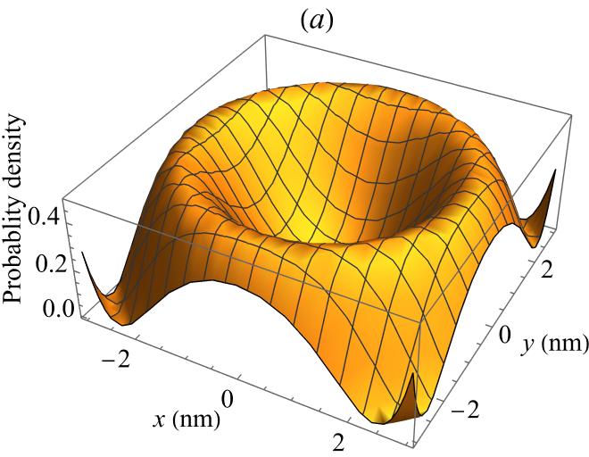
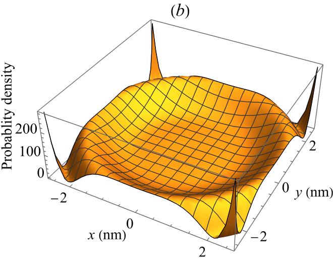
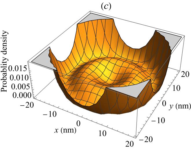
Figure 1: (Color online) The probability distribution for two particles calculated with ($a$) the Kratzer potential (1), ($b$) the modified Kratzer’s potential (2) for interactions of diatomic molecules, ($c$) the modified Kratzer’s potential (3) for an electron-hole interaction. Calculations are performed for $n=3$ and $m=1$.

VI Conclusion

One of the challenging tasks of quantum mechanics in two-dimension is to find the exact analytical solution of the Schrödinger equation for a given potential and any arbitrary value $m$ in 2D configuration spaces. This solution can be further used to define the observables of the system.

In this study, we found the exact bound state solutions of the two–dimensional Schrödinger equation with Kratzer–type potentials and present analytical expressions for the eigenvalues and eigenfunctions. The eigenfunctions are given in terms of the associated Laguerre polynomials.

References

- (1) L. D. Landau and E. M. Lifshitz, Quantum Mechanics (Non-relativistic Theory) 3rd ed. ~Pergamon, Oxford, 1977.
- (2) L. I. Schiff, Quantum Mechanics, 4th Edition, McGraw Hill Education, 2014.
- (3) A.S. Davydov, Quantum Mechanics, Pergamon, Oxford and New York, 1965; Moscow, 1973
- (4) J. J. Sakurai, Modern Quantum Mechanics, Benjamin, New York, 1985.
- (5) S. Flügge, Practical Quantum Mechanics. Berlin, Springer, 1971.
- (6) R. W. Robinett, Quantum Mechanics: Classical Results, Modern Systems, and Visualized Examples. 2nd ed., Oxford University Press, 2006.
- (7) D. J. Griffiths, D. F. Schroeter, Introduction to Quantum Mechanics 3rd Edition, Cambrige University Press, 2018.
- (8) L. Ellis, I. Ellis, C. Koutschan, and S. K. Suslov, On potentials integrated by the Nikiforov-Uvarov method. arXiv:2303.02560v4 [quant-ph] (2023).
- (9) A. Gugiuzza, A. Politano, and E. Drioli, The advent of graphene and other two–dimensional materials in membrane science and technology, Curr. Opin. Chem. Eng. 16, 78 (2017).
- (10) S. Wachter and D. K. Polyushkin, O. Bethge, and T. Mueller, A microprocessor based on a two–dimensional semiconductor, Nat. Commun. 8, 14948 (2017).
- (11) K. S. Novoselov and A. K. Geim and S. V. Morozov and D. Jiang and Y. Zhang and S. V. Dubonos and I. V. Grigorieva and A. A. Firsov, Electric field effect in atomically thin carbon films, Science. 306, 5696 (2004).
- (12) R.F. Frindt, Single crystals of MoS2 several molecular layers thick, Journal of Applied Physics, 37, 4, 1928-1929 (2004).
- (13) K. F. Mak, C. Lee, J. Hone, J. Shan, and T. F. Heinz, Atomically thin MoS2: A new direct-gap semiconductor, Phys. Rev. Lett. 105, 136805 (2010).
- (14) M. Li, and X. C. Zeng, Group IVB transition metal trichalcogenides: A new class of 2D layered materials beyond graphene, WIREs Comput. Mol. Sci. 6, 211 (2016).
- (15) P. Avouris, T. F. Heinz, and T. Low, 2D materials: Properties and devices (Cambridge University Press, 2017).
- (16) R. Cheng, D. Li, H. Zhou, C. Wang, A. Yin, S. Jiang, Y. Liu, Y. Chen, Y. Huang, and X. Duan, Electroluminescence and photocurrent generation from atomically sharp WSe2/MoS2 heterojunction p{n diodes, Nano Lett. 14, 5590 (2014).
- (17) C.-H. Lee, G.-H. Lee, A. Zande, W. Chen, Y. Li, M. Han, X. Cui, G. Arefe, C. Nuckolls, T. Heinz, et al., Atomically thin p{n junctions with van der Waals heterointerfaces, Nat. Nanotechnol. 9, 676 (2014).
- (18) O. Cotlet , S. Zeytino glu, M. Sigrist, E. Demler, and A. Imamo glu, Superconductivity and other collective phenomena in a hybrid Bose-Fermi mixture formed by a polariton condensate and an electron system in two dimensions, Phys. Rev. B 93, 054510 (2016).
- (19) S. Manzeli, D. Ovchinnikov, D. Pasquier, O. V. Yazyev, and A. Kis, 2D transition metal dichalcogenides, Nat. Rev. Mater. 2, 17033 (2017).
- (20) O. L. Berman and R. Ya. Kezerashvili, High-temperature superfuidity of the two-component Bose gas in a transition metal dichalcogenide bilayer, Phys. Rev. B 93, 245410 (2016).
- (21) O. L. Berman and R. Ya. Kezerashvili, Superuidity of dipolar excitons in a transition metal dichalcogenide double layer, Phys. Rev. B 96, 094502 (2017).
- (22) G. Wang, A. Chernikov, M. M. Glazov, T. F. Heinz, X. Marie, T. Amand, and B. Urbaszek, Colloquium: Excitons in atomically thin transition metal dichalcogenides, Rev. Mod. Phys. 90, 021001 (2018).
- (23) M. N. Brunetti, O. L. Berman, and R. Ya. Kezerashvili, Optical absorption by indirect excitons in a transition metal dichalcogenide/hexagonal boron nitride heterostructure, J. Phys.: Condens. Matter 30, 225001 (2018).
- (24) R. Ya. Kezerashvili and A. Spiridonova, Magnetoexcitons in transition metal dichalcogenides monolayers, bilayers, and van der Waals heterostructures, Phys. Rev. Res. 3, 033078 (2021).
- (25) A. Kratzer, Die ultraroten rotationsspektren der halogenwasserstoffe. Z. Physik 3, 289 (1920); E. Fues, Das eiegenschewingungaspekrum zweiatomiger moleküle in der undulationsmechanik. Ann. Phys. 80, 367 (1926).
- (26) R. J. LeRoy and R. B. Bernstein, Dissociation energy and long-range potential of diatomic molecules from vibrational spacings of higher levels. J.Chem. Phys. 52, 3869 (1970).
- (27) C. Berkdemir, A. Berkdemir, and J. Han, Bound state solutions of the Schrödinger equation for modified Kratzer’s molecular potential, Chem. Phys. Lett. 417, 326 (2006).
- (28) M. R. Molas, et al., Energy spectrum of two–dimensional excitons in a nonuniform dielectric medium. Phys. Rev. Let. 123, 136801 (2019).
- (29) R. Ya. Kezerashvili, Few-body systems in condensed matter physics, Few Body Syst. A 60, 52 (2019).
- (30) R. Ya. Kezerashvili, Trions in three–, two– and one–dimensional materials. Recent Progress in Few-Body Physics 238, 825 (2020). In: Orr, N., Ploszajczak, M., Marqués, F., Carbonell, J. (eds) Recent Progress in Few-Body Physics. FB22 2018. Springer Proceedings in Physics, 238. 825 (2020).
- (31) A. F. Nikiforov and V. B. Uvarov, Special Functions of Mathematical Physics. A Unified Introduction with Applications. Springer Basel AG, 1988.
- (32) R. Ya. Kezerashvili, J. Luo, C. R. Malvino, On an exactly solvable two-body problem in two–dimensional quantum mechanics. Few-Body Syst. 64, 79 (2023).
- (33) S. B. Doma, A. A. Gohar, and M. S. Younes, Analytical solutions of the molecular Kratzer-Feus potential by means of the Nikiforov-Uvarov method. J. Math. Chem. 61, 1301 (2023).
- (34) P. M. Morse and H. Feshbach, Methods of Theoretical Physics, McGraw-Hll Book Company, 1953.
- (35) B. Zaslow and M. E. Zandler, Two-dimensional analog of the hydrohen atom. Am. J. Phys. 35, 1118 (1967).
- (36) I. S. Gradshteyn and I. M. Ryzhik, Table of Integrals, Series, and Products, 7th Edition, Elsevier, Amsterdam 2007.
- (37) Handbook of Mathematical Functions With Formulas, Graphs, and Mathematical Tables, edited by M. Abramowitz and I. A. Stegun, NBS Applied Mathematics Series 55, National Bureau of Standards, Washington, 1964.
- (38) A. D. Polyanin and V. F. Zaitsev, Handbook of Oridinary Differential Equations, Exact Solutions, Methods, and Problems, CRC Press, Taylor & Francis Group, 2018.
- (39) X. L. Yang, S. H. Guo, F. T. Chan, K. W. Wong, and W. Y. Ching, Analytical solution of a two–dimensional hydrogen atom. I. Nonrelativistic theory. Phys. Rev. A 43, 1186 (1991).
- (40) D. G. W. Parfitt and M. E. Portnoi, The two–dimensional hydrogen atom revisited. J. Mat. Phys. 43, 4681 (2002).