Energy-dependent implementation of secondary electron emission models in continuum kinetic sheath simulations

Abstract

The plasma-material interactions present in multiple fusion and propulsion concepts between the flow of plasma through a channel and a material wall drive the emission of secondary electrons. This emission is capable of altering the fundamental structure of the sheath region, significantly changing the expected particle fluxes to the wall. The emission spectrum is separated into two major energy regimes, a peak of elastically backscattered primary electrons at the incoming energy, and cold secondary electrons inelastically emitted directly from the material. The ability of continuum kinetic simulations to accurately represent the secondary electron emission is limited by relevant models being formulated in terms of monoenergetic particle interactions which cannot be applied directly to the discrete distribution function. As a result, rigorous implementation of energy-dependent physics is often neglected in favor of simplified, constant models. We present here a novel implementation of semi-empirical models in the boundary of continuum kinetic simulations which allows the full range of this emission to be accurately captured in physically-relevant regimes.

I Introduction

Continuum kinetic models of plasmas allow simulations to capture the distribution function dynamics at small-scale processes, while avoiding the statistical noise that poses problems for particle-in-cell (PIC) methods [1]. When applied to the situation of the classical plasma sheath which forms at the boundary of a plasma and a material surface, continuum kinetics allows for accurate simulation of the sheath region and instabilities [2, 3]. However, the addition of secondary electron emission (SEE) physics poses several unique challenges to these models. The ability to simulate SEE rigorously in continuum kinetic codes is heavily restricted by the need to apply emission models which describe monoenergetic particle interactions to the discrete distribution function. These codes are unable to sample the emitted distribution for individual impact events using Monte Carlo methods as particle codes do [4, 5], and struggle to represent the full range of emission behaviors across all incoming energies. These restrictions often lead to oversimplified or constant implementations of complex physics, which, while sufficient for examining behavior in specific regimes, fail to capture the dynamic nature of actual physical applications. Presented in this work is an overview of different approaches to modeling the SEE, discussion of their limitations, and novel implementation of phenomenological models in a continuum kinetic framework.

II Emitting Sheaths

The plasma sheath forms due to the greater mobility of the electrons over ions. Greater electron current at the surface causes a negative potential to develop, which drives the formation of a positive space-charge region near the material. Ions are accelerated while electrons are repelled, leading to an equalization of the fluxes at the wall. The characteristic length scale in the sheath is the Debye length,

$$\lambda_{D}=\sqrt{\frac{\varepsilon_{0}k_{B}T_{e}}{n_{e}q_{e}^{2}}},$$ (1)

where $\varepsilon_{0}$ is the vacuum permittivity, $k_{B}$ is the Boltzmann constant, $T_{e}$ is the electron temperature, $n_{e}$ is the electron number density, and $q_{e}$ is electron charge. The length of the sheath region is typically on the order of some tens of Debye lengths. At the sheath entrance, ions must be accelerated to the Bohm speed $u_{B}$. Several formulations of this resulting Bohm sheath criterion are possible [6, 7, 8], but the one used for the purposes of this work has the form [9]

$$u_{i}\geq u_{B}=\sqrt{\frac{k_{B}T_{e}+\gamma k_{B}T_{i}}{m_{i}}},$$ (2)

where $u_{i}$ is the ion drift speed in the sheath, and $\gamma$ is the heat capacity ratio.

The above overview of the theory assumes the wall perfectly absorbs any particles which impact it. In physical cases, however, impact of energetic “primary” electrons leads to the emission of the so-called “secondary” electrons from the wall material into the sheath, considerably impacting the resulting physics. The emission of secondary electrons also occurs with the impact of primary ions. We define the secondary electron yield (SEY) to be the number of secondary particles emitted per primary particle impact. The SEY of a surface depends on material properties and the energy and angle of the primary particle. For low SEY below unity, the sheath will remain “classical”; that is, monotonic with a negative wall potential. At some critical SEY near unity, the sheath potential becomes non-monotonic and transitions to a space-charge limited (SCL) sheath [10, 11]. Theory further predicts that when the ratio of emitted flux to flux from the bulk plasma exceeds unity, ion collisional effects will drive the SCL sheath to a reverse sheath where the wall potential is positive relative to the sheath entrance [12, 13].

Modifications can be made to the sheath theory to account for the presence of particle emission [10, 11, 12, 14]. These models, however, generally invoke simplifying assumptions about the emitted particle distribution, considering it to be constant, cold, and half-Maxwellian, typical of thermionic probe emission. The emission of a material under particle impact, however, is significantly more dynamic and varied. Measurements of the SEE spectrum for various materials under electron impact show three distinct populations of emitted particles [15]. A peak is located at the incident energy representing particles which reflect approximately elastically off the wall. A peak at low energy represents the so-called “true” secondary electrons emitted from the material. The low emission region between these two contains the inelastically reflected, or rediffused particles, which penetrate the surface but undergo several scattering events and are reemitted at lower energy.

III Numerical Model

III.1 The Kinetic Equations

The core kinetic model is the Vlasov-Maxwell-Fokker-Planck (VM-FP) system of equations, coupling Maxwell’s equations with the Boltzmann equation

$$\frac{\partial f_{s}}{\partial t}=-\mathbf{v}\cdot\frac{\partial f_{s}}{\partial\mathbf{x}}-\frac{q_{s}}{m_{s}}(\mathbf{E}-\mathbf{v}\times\mathbf{B})\cdot\frac{\partial f_{s}}{\partial\mathbf{v}}+\bigg{(}\frac{\partial f_{s}}{\partial t}\bigg{)}_{c},$$ (3)

where $f_{s}$ is the particle distribution function for species $s$. In this work, Coulomb collisions are represented by the Lenard-Bernstein (LBO) collision operator [16]. This operator takes the form

$$\bigg{(}\frac{\partial f_{s}}{\partial t}\bigg{)}_{c}=\sum_{r}\nu_{sr}\frac{\partial}{\partial\mathbf{v}}\cdot\left[(\mathbf{v}-\mathbf{u}_{sr})f_{s}+v_{t,sr}^{2}\frac{\partial f_{s}}{\partial\mathbf{v}}\right],$$ (4)

where $\nu_{sr}$ is the collision frequency with species $r$ and $v_{t,sr}$ is the cross-flow thermal velocity.

In this work, the discretization of the distribution function and evolution of Eq. 3 is done using the discontinuous Galerkin (DG) numerical method [17] with the Gkeyll software [18]. It is nevertheless our intent that this algorithm be generally applicable to variety of computational methods. Therefore, while some of the DG details will be given where necessary, the work shown here should be valid for any numerical discretization technique. The Gkeyll code employs a multistage Runge-Kutta (RK) scheme of successive forward Euler steps, described in Alg. 1, but the general procedure of calculating the right-hand side (RHS) terms of Eq. 3 and advancing them by some time step is common to all relevant schemes.

// Calculation of VM-FP RHS terms

$\mathcal{L}=\frac{\partial f^{n}}{\partial t}$

// Forward Euler update

$\mathcal{F}=f^{n}+\Delta t\mathcal{L}$

// RK stage update

$f^{n+1}=$ rkStage($f^{n},\mathcal{F}$)

// Calculation of ghost cell distribution from skin cell distribution

$f^{g,n+1}=$ bcCalc($f^{s,n+1}$)

Algorithm 1 Continuum kinetic update algorithm

Of particular relevance to this work are the skin and ghost cells. The ghost cells are a set of cells place outside the edge of the domain which are set by the boundary condition in the previous time step, and are used in the RHS update of the interior cell layer bordering the domain edge (the “skin” cells) during the DG update. In most cases dealing with particle emission, the ghost cell distribution calculated by the boundary condition will depend on the incoming distribution in the skin cells [19].

A thorough outline of the full DG discretization of the VM-FP system is presented in [20, 21, 22, 23, 24]. As this paper deals extensively with transformations of the discrete distribution function, the weak formulation is described in the following section.

III.2 The Discrete Distribution Function

The distribution function $f(\mathbf{x},\mathbf{v})$ and the discrete distribution function $f_{h}(\mathbf{x},\mathbf{v})$ are related through weak equality $f(\mathbf{x},\mathbf{v})\circeq f_{h}(\mathbf{x},\mathbf{v})$, that is

$$\begin{split}\int_{\mathcal{X}}\int_{\mathcal{V}}f(\mathbf{x},\mathbf{v})\psi_{t}(\mathbf{x},\mathbf{v})d\mathbf{x}d\mathbf{v}\\ =\int_{\mathcal{X}}\int_{\mathcal{V}}f_{h}(\mathbf{x},\mathbf{v})\psi_{t}(\mathbf{x},\mathbf{v})d\mathbf{x}d\mathbf{v},\end{split}$$ (5)

where $\psi_{t}(\mathbf{x},\mathbf{v})$ is the test function. To evaluate the discrete distribution function, we do a coordinate transformation from phase space ($\mathcal{X},\mathcal{V}$) with ($\mathbf{x},\mathbf{v}$) coordinates to logical space $\mathcal{I}$ with ($\bm{\eta}_{\mathbf{x}},\bm{\eta}_{\mathbf{v}}$) coordinates spanning the range $-1$ to $1$ in each dimension in each cell,

$$x_{i}(\eta_{i})=\eta_{i}\frac{\Delta x_{i}}{2}+x_{ci},\quad-1\leq\eta_{i}\leq 1.$$ (6)

Here, $x_{ci}$ is the cell center value, and $\Delta x_{i}$ is the cell width. We take the discrete distribution function in each cell to be the sum of $N_{b}$ expansion coefficients ($\hat{f}=[\hat{f}_{0},\hat{f}_{1},...,\hat{f}_{N_{b}-1}]$) and basis functions ($\hat{\psi}(\bm{\eta}_{\mathbf{x}},\bm{\eta}_{\mathbf{v}})=[\hat{\psi}_{0}(\bm{\eta}_{\mathbf{x}},\bm{\eta}_{\mathbf{v}}),\hat{\psi}_{1}(\bm{\eta}_{\mathbf{x}},\bm{\eta}_{\mathbf{v}}),...,\hat{\psi}_{N_{b}-1}(\bm{\eta}_{\mathbf{x}},\bm{\eta}_{\mathbf{v}})]$).

Thus, the representation of the distribution function in cell $i$ in configuration space and $j$ in velocity space is

$$f^{ij}(\mathbf{x},\mathbf{v}) \circeq f^{ij}_{h}(\mathbf{x},\mathbf{v}),\quad\mathbf{x},\mathbf{v}\in\mathcal{X}^{i},\mathcal{V}^{j}$$ (7)

$$=\sum_{k=0}^{N_{b}-1}\hat{f}^{ij}_{k}\hat{\psi}_{k}(\bm{\eta}_{\mathbf{x}},\bm{\eta}_{\mathbf{v}}).$$

This results in Eq. 5 becoming

$$\mathbf{M}\hat{f}^{ij}=\int_{\mathcal{I}}f\big{(}\mathbf{x}(\bm{\eta}_{\mathbf{x}}),\mathbf{v}(\bm{\eta}_{\mathbf{v}})\big{)}\psi_{t}(\bm{\eta}_{\mathbf{x}},\bm{\eta}_{\mathbf{v}})d\bm{\eta}_{\mathbf{x}}d\bm{\eta}_{\mathbf{v}},$$ (8)

where

$$\mathbf{M}=\int_{\mathcal{I}}\hat{\psi}(\bm{\eta}_{\mathbf{x}},\bm{\eta}_{\mathbf{v}})\psi_{t}(\bm{\eta}_{\mathbf{x}},\bm{\eta}_{\mathbf{v}})d\bm{\eta}_{\mathbf{x}}d\bm{\eta}_{\mathbf{v}}$$

is the mass matrix, and the expressions $\mathbf{x}(\bm{\eta}_{\mathbf{x}})$, $\mathbf{v}(\bm{\eta}_{\mathbf{v}})$ are taken from Eq. 6. In Gkeyll, we choose the same orthonormal polynomial basis set for both the basis functions $\hat{\psi}(\bm{\eta}_{\mathbf{x}},\bm{\eta}_{\mathbf{v}})$ and the test functions $\psi_{t}(\bm{\eta}_{\mathbf{x}},\bm{\eta}_{\mathbf{v}})$. This orthonormality causes the mass matrix $\mathbf{M}=\mathbf{I}_{b},$ where $\mathbf{I}_{b}$ is the $N_{b}\times N_{b}$ identity matrix. The integral on the right-hand side of of Eq. 8 can be evaluated numerically to obtain the DG expansion coefficients of the discrete distribution function.

IV Secondary Electron Emission Models

The models discussed in this work deal exclusively with electron-impact SEE. Ion-impact SEE is also possible in regimes of high energy ions, and models for these interactions will be addressed in detail in future related work. The fundamental algorithms here, however, are agnostic to whether the impacting and emitted species are the same. We take the subscript $\alpha$ to denote the particle species impacting the wall, and $\beta$ to denote the species being emitted. We further denote the energy of an impacting particle $E^{\prime}$ with angle cosine $\mu^{\prime}$, and the emitted particle energy $E$ with angle cosine $\mu$. Energetic quantities are all in electronvolts (eV). These parameters are related directly to the particle velocity.

$$E_{s}=\frac{1}{2}\frac{m_{s}}{q_{0}}\mathbf{v}\cdot\mathbf{v},$$ (9)

$$\mu=\frac{\mathbf{n}\cdot\mathbf{v}}{|\mathbf{v}|},$$ (10)

with $q_{0}$ being elementary charge, and $\mathbf{n}$ being the unit vector normal to the wall. Typically in this work, emission models will be formulated in terms of $E$ and $\mu$, while distribution functions will be expressed in terms of $\mathbf{v}$.

We further define the secondary electron yield (SEY) to be the ratio of the emitted particle flux to the impacting particle flux $\delta=\Gamma_{\beta}^{-}/\Gamma_{\alpha}^{+}$. For this work, the positive direction is defined as into the wall, the negative direction as out of the wall.

In this work we treat the populations separately, denoting the elastic yield as $\delta_{e}$, and the true secondary yield as $\delta_{ts}$. The rediffusion, $\delta_{r}$, will not be implemented by this work as it minimally contributes in most situations to the overall emitted population and presents unique modeling difficulties. Typically, at lower energies backscattering dominates emission, while true secondary emission dominates high energy situations. As will be shown, neither stand completely independent in any regime.

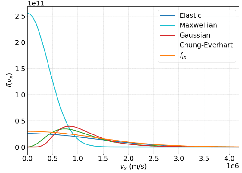
Figure 1: Comparison of different secondary electron emission spectrums when $\delta=0.85$. While the flux ratio is constant across each case, the resulting densities are quite different. When the emitted particles are at low energy, they pile up significantly more at the wall than emission spectrums with high velocity tails.

IV.1 Constant Emission

The simplest means of extending constant emission to an inelastic emission spectrum is to scale a representative curve by a normalization factor $C$, such that

$$f^{g}_{\beta}(\mathbf{x},\mathbf{v})=Cf_{ts}(\mathbf{v}).$$ (11)

Here $f_{ts}(\mathbf{v})$ is the function for the emission spectrum, and $C$ is a normalization factor that ensures the flux ratio is correct. The simplest approach is elastic emission, setting $C=\delta_{e}$ and $f_{ts}(\mathbf{v}^{-})=f_{\alpha}^{s}(\mathbf{x}_{wall},\mathbf{v}^{+})$.

An inelastic implementation for the true secondary population is more sophisticated, using the impacting flux to scale some emission spectrum function. From the definition of $\delta_{ts}$ using the ratio of flux/first moment,

$$C=\frac{\delta_{ts}\Gamma_{\alpha}^{+}}{\int_{\mathcal{V}^{-}}\mathbf{n}\cdot\mathbf{v}f_{ts}(\mathbf{v})d\mathbf{v}}.$$ (12)

The denominator can be solved analytically for a chosen $f_{ts}(\mathbf{v})$ spectrum. For a Maxwellian

$$f_{ts}(\mathbf{v})=\exp{\bigg{(}-\frac{\mathbf{v}\cdot\mathbf{v}}{2v_{emit}^{2}}\bigg{)}},$$ (13)

this expression yields

$$C_{M}=\frac{\delta_{ts}\Gamma_{\alpha}^{+}}{(2\pi)^{\frac{d_{v}-1}{2}}v_{emit}^{d_{v}+1}},$$ (14)

for dimensions $d_{v}$ in velocity space.

Here, $v_{emit}=\sqrt{\frac{k_{B}T_{emit}}{m_{e}}}$ will typically be chosen with a cold $T_{emit}$ to match standard true secondary electron emission behavior.

Other spectrum function choices are available and supported by emission data, such as the Gaussian function [25]

$$f_{ts}(\mathbf{v})=\exp{\bigg{(}-\frac{\ln{\big{(}\frac{E(\mathbf{v})}{E_{0}}\big{)}}^{2}}{2\tau^{2}}\bigg{)}},$$ (15)

where $E_{0}$ and $\tau$ are fitting parameters, and the Chung-Everhart [26] model

$$f_{ts}(\mathbf{v})=\frac{E(\mathbf{v})}{(E(\mathbf{v})+\phi)^{4}},$$ (16)

where $\phi$ is the material work function (or electron affinity for insulators). The fluxes of these functions do not give analytical solutions which scale cleanly into higher dimensions (see Section VI-A), but in 1V the solutions are

$$C_{G}=\frac{\delta_{ts}\Gamma_{\alpha}^{+}m_{\beta}}{\sqrt{2\pi}q_{0}E_{0}\tau\exp{(\tau^{2}/2)}},$$ (17)

and

$$C_{CE}=\frac{6m_{\beta}}{q_{0}}\phi^{2}\delta_{ts}\Gamma_{\alpha}^{+},$$ (18)

for the Gaussian and Chung-Everhart functions, respectively.

Comparisons of how the choice of spectrum changes the emission for the same yield value are shown in Fig. 1. Despite having the same flux ratio, the resulting distribution is vastly different. Particles at high velocity contribute more to emission than particles at low velocity, so the Maxwellian centered at zero emits at far greater density than the other curves.

There are two drawbacks in using either constant elastic or inelastic emission, or some combination of the two. First, as these $\delta$ values are constant across space, low energy particles nonphysically contribute to the cold secondaries, and conversely there is nonphysical backscattering of high energy particles back into the sheath. Second, any constant application of the yield across space also results in a necessarily constant yield in time; and as such, the implementation does not capture any feedback between the emission and the sheath.

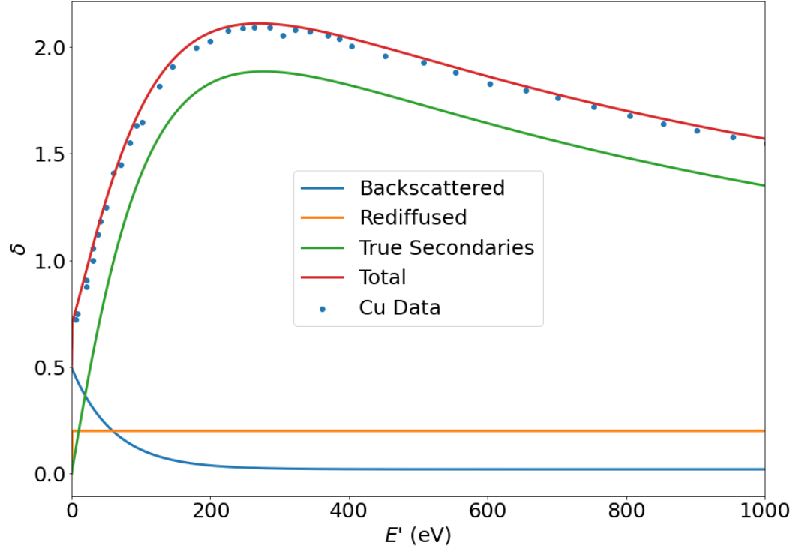
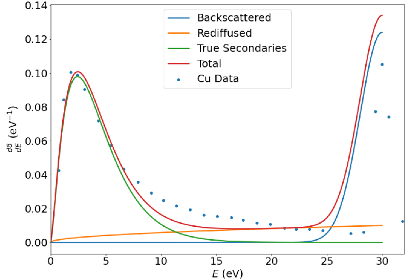
Figure 2: Emission data [27] for copper yield (top) and $30\text{\,}\mathrm{e}\mathrm{V}$ beam emission spectrum (bottom) with Furman-Pivi fits [28] to the three populations of secondary electrons. There is a near-elastic peak at the beam energy which corresponds to the backscattering, while regardless of beam energy the location of the true secondary peak will remain approximately the same.

IV.2 Furman-Pivi Model

The Furman-Pivi model [28] gives the SEE emission spectrum for a monoenergetic beam of impacting electrons; thus, $\alpha$ and $\beta$ are both electrons. There are two parts to the Furman-Pivi model. The SEY which gives the number of particles emitted per incident particle,

$$\delta_{tot}(E^{\prime},\mu^{\prime})=\delta_{e}(E^{\prime},\mu^{\prime})+\delta_{r}(E^{\prime},\mu^{\prime})+\delta_{ts}(E^{\prime},\mu^{\prime}),$$ (19)

and the spectrum which describes how the emitted particles are distributed across outgoing energy,

$$\begin{split}\frac{\partial\delta_{tot}}{\partial E}\bigg{(}E,E^{\prime},\mu^{\prime}\bigg{)}=\frac{\partial\delta_{e}}{\partial E}\bigg{(}E,E^{\prime},\mu^{\prime}\bigg{)}\\ +\frac{\partial\delta_{r}}{\partial E}\bigg{(}E,E^{\prime},\mu^{\prime}\bigg{)}+\frac{\partial\delta_{ts}}{\partial E}\bigg{(}E,E^{\prime},\mu^{\prime}\bigg{)}.\end{split}$$ (20)

These fits are shown for copper data in Fig. 2. As mentioned, we are neglecting the rediffused population represented by $\delta_{r}$, $\frac{\partial\delta_{r}}{\partial E}$. Additionally, while the Furman-Pivi model give a spectrum for the backscattered population, we note that the backscattering can be approximated well as purely elastic, and thus drop $\frac{\partial\delta_{e}}{\partial E}$ as a full spectrum implementation. Discussion here will focus therefore on the implementation of the true secondary population. The separate handling of elastic backscattering terms is discussed in Section IV-C.

The Furman-Pivi fit to the SEY curve is

$$\delta_{ts}(E^{\prime},\mu^{\prime})=\hat{\delta}(\mu^{\prime})D(E^{\prime}/\hat{E}(\mu^{\prime})),$$ (21)

$$\hat{\delta}(\mu^{\prime})=\hat{\delta}_{ts}[1+t_{1}(1-\mu^{\prime t_{2}})],$$ (22)

$$\hat{E}=\hat{E}_{ts}[1+t_{3}(1-\mu^{\prime t_{4}})],$$ (23)

$$D(x)=\frac{sx}{s-1+x^{s}},$$ (24)

where $\hat{\delta}_{ts}$, $\hat{E}_{ts}$, $s$, $t_{1}$, $t_{2}$, $t_{3}$, and $t_{4}$ are fitting parameters.

The emission spectrum for the true secondary electrons is expressed by

$$\begin{split}\frac{\partial\delta_{ts}}{\partial E}\bigg{(}E,E^{\prime},\mu^{\prime}\bigg{)}=\sum_{n=1}^{M}\frac{nP_{n,ts}(E^{\prime},\mu^{\prime})(E/\varepsilon_{n})^{p_{n}-1}\exp{(-E/\varepsilon_{n})}}{\varepsilon_{n}\Gamma(p_{n})P(np_{n},E^{\prime}/\varepsilon_{n})}P\big{(}(n-1)p_{n},(E^{\prime}-E)\varepsilon_{n}\big{)},\end{split}$$ (25)

$$P_{n,ts}(E^{\prime},\mu^{\prime})=\binom{M}{n}\Bigg{(}\frac{\delta_{ts}(E^{\prime},\mu^{\prime})}{M}\Bigg{)}^{n}\Bigg{(}1-\frac{\delta_{ts}(E^{\prime},\mu^{\prime})}{M}\Bigg{)}^{M-n},$$ (26)

where $p_{n}$, $\epsilon_{n}$, are fitting parameters determined from beam data. $\Gamma(\cdot)$ is the delta function, and $P(\cdot,\cdot)$ is the normalized incomplete delta function. The summation is of the probability $n$ secondary electrons up to a total of $M$ being emitted. $M$ theoretically goes to infinity, but $M=10$ is sufficient for high accuracy.

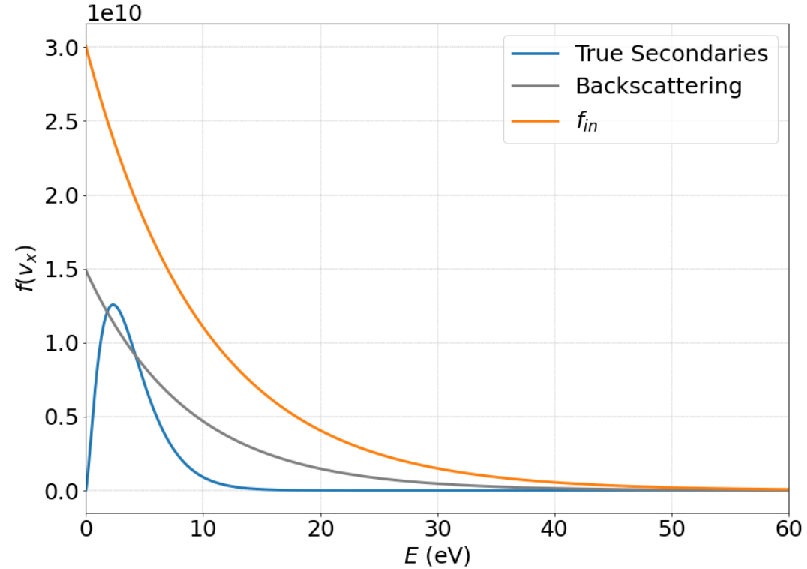
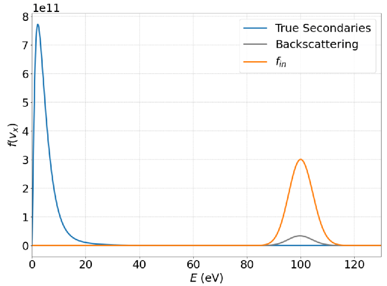
Figure 3: Plot with the elastic and inelastic emission curves in the low (left) and high (right) energy regimes. At low energy, backscattering contributes significantly and the total emission is concentrated at low energy where the incoming distribution is. For the high energy beam, the true secondary distribution dominates emission but there is a small elastic peak at the beam energy.

There can be a fair amount of variance in the emission data curves for materials depending on methodology and treatment of the material prior to testing [27, 29, 30]; for simplicity’s sake, here we use the copper parameters calculated by Furman & Pivi in Table 1 of [28], used for the fits in Fig. 2. Fits of this same model can be done to any desired dataset, however.

The Furman-Pivi model describes the emission of a monoenergetic beam. To apply this to a continuous impacting distribution, simplifications must be made. We can obtain the cumulative emission curve of an incoming distribution by generating a unique emission spectrum for a wide range of incoming points $\mathbf{v}^{\prime}$ along the distribution and summing these emission spectrums to get the total. The individual emission spectrum can be determined from $\frac{\partial\delta}{\partial E}$ by using the definition of yield as the ratio of fluxes.

This relation can be written as

$$\begin{split}\int_{\mathcal{V}^{-}_{\beta}}\mu(\mathbf{v})\frac{\partial\delta}{\partial E}\bigg{(}E(\mathbf{v}),E^{\prime}(\mathbf{v}^{\prime}),\mu^{\prime}(\mathbf{v})\bigg{)}\mathcal{J}_{E,\mu}(\mathbf{v})d\mathbf{v}\\ =\frac{\int_{\mathcal{V}_{\beta}^{-}}\mathbf{n}\cdot\mathbf{v}f_{ts}(\mathbf{v})d\mathbf{v}}{\mathbf{n}\cdot\mathbf{v}^{\prime}f_{in}(\mathbf{x}_{wall},\mathbf{v}^{\prime})d\mathbf{v}},\end{split}$$ (27)

where $\mathcal{J}_{E,\mu}(\mathbf{v})=\left|\frac{\partial(E,\mu)}{\partial(\mathbf{v})}\right|$ is the Jacobian matrix for the coordinate transformation. This simplifies in 1V for $v_{x}$ to give us the emission spectrum for each incoming monoenergetic beam,

$$f_{ts}(v_{x})=\frac{m_{e}}{q_{0}}\frac{\partial\delta}{\partial E}\bigg{(}E(v_{x}),E^{\prime}(v^{\prime}_{x}),\mu^{\prime}=1\bigg{)}v^{\prime}_{x}f_{in}(x_{wall},v^{\prime}_{x})dv_{x}.$$ (28)

Fig. 3 demonstrates the application of this calculation to two distributions, one a high energy $100\text{\,}\mathrm{e}\mathrm{V}$ beam, the other a cold Maxwellian with a temperature of $10\text{\,}\mathrm{e}\mathrm{V}$. Also included in the figures are the backscattered spectrums, which will be discussed in greater depth in Section IV-C. There are two primary features we would draw attention to. First, the location and width of the secondary electron emission distribution do not change significantly based on the incoming energy range, only the magnitude of the emitted spectrum. Second, we would note that even for the cold distribution where we expect emission of true secondaries to be low, the high energy tail is sufficiently populated to create a significant emitted distribution.

Instead of implementing the Furman-Pivi spectrum directly into the software, as it is mathematically complicated and computationally expensive to compute during run time, we instead will substitute one of the $f_{ts}(\mathbf{v})$ equations from the previous section and use the full Furman-Pivi only for purposes of comparing model accuracy. As the Maxwellian is less accurate to observed emission data, we will only look at the Gaussian and Chung-Everhart models. The key step here is that Eq. 21, the energy-dependent Furman-Pivi SEY equation, is substituted in for $\delta_{ts}$ in the calculation of the normalization factors from the solutions of Eq. 12, ensuring that the total yield remains the same (“conserved” during the spectrum substitution) despite the simpler spectrum model.

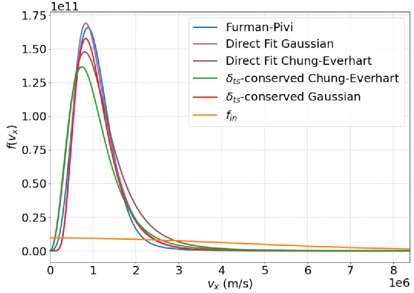
Figure 4: Comparison of several different options for the cumulative true secondary emission spectrum of a $T_{e}=$100\text{\,}\mathrm{e}\mathrm{V}$$, $n_{e}=$1.0\text{\times}{10}^{17}\text{\,}\mathrm{m}^{-3}$$ Maxwellian. Direct fits match the theoretical Furman-Pivi spectrum quite well, but the overestimation of the high velocity tail is consequential when looking at the total yield (see Fig. 5).

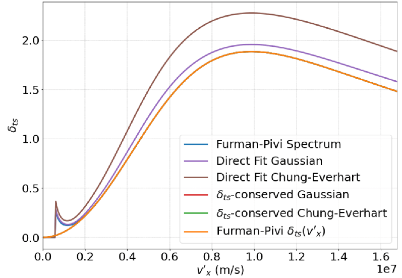
Figure 5: Comparison of the Furman-Pivi yield curve to total yield obtained by integrating to get the emission spectrum flux for a range of incoming energies. The $\delta$-conserving models are, as expected, exact to the Furman-Pivi yield curve. The Furman-Pivi spectrum and fits directly to it diverge at very low energy from the theory, as the Furman-Pivi fitting parameters are obtained from high energy beam data. Fits directly to Furman-Pivi overshoot the total yield.

Fig. 4 shows these spectrums for an incoming Maxwellian with an electron temperature of $100\text{\,}\mathrm{e}\mathrm{V}$. In addition to the $\delta_{ts}$-conserving models, direct fits of the Gaussian and Chung-Everhart to the Furman-Pivi distribution are shown for comparison. While these direct fits are closer in terms of overall error in the distribution from the Furman-Pivi curve, the excess in the higher velocity region causes them to considerably overshoot the total yield, as shown in Fig. 5. The SEY curves in Fig. 5 are obtained by integrating over each unique emission spectrum produced by an incoming $v_{x}^{\prime}$ point to get the outgoing flux, and taking the ratio with the incoming flux $v^{\prime}_{x}f_{in}(v^{\prime}_{x})dv_{x}$. When compared to Eq. 21, the yield conserving cases do, as expected, match perfectly to the theoretical SEY curve. Curiously, at very low energies the theoretical Furman-Pivi emission spectrum does not, and indeed must be cut off to avoid a sharp increase near zero. This is not actually so surprising given that the Furman-Pivi spectrum fitting parameters are obtained from high energy data. These work extremely well for the majority of the energy range, but there is a particular dearth of emission data at very low energies, and in this region they begin to break down. As the direct fit curves are done to the theoretical Furman-Pivi spectrum, they share this quirk. It should be noted that since yield is based on flux, not density, low energy particles only contribute a minor amount compared to the high-velocity tail of the distribution, so this divergence is not particularly bothersome in any case.

Overall, the Gaussian provides a better match to the emission spectrum, but the Chung-Everhart bears a distinct advantage. It’s sole fitting parameter, $\phi$, is the material work function, and thus can be determined adequately without any emission spectrum data. The Gaussian, on the other hand, requires estimates of $E_{0}$ and $\tau$. $E_{0}$ represents the peak location, which can in a pinch be approximated per Chung & Everhart as $\phi/3$ [26]. However, $\tau$ can only be estimated by some fit to existing spectrum data, which can be quite rare and not readily available for some materials.

In either case, however, adopting this simple modelling method of swapping out the complicated spectrum fit while relying on the fits to SEY data gives us fairly accurate representations of the emitted spectrums which perfectly conserve the total yield.

IV.3 Elastic Model

For elastic emission $E=E^{\prime}$, $\mu=\mu^{\prime}$. Thus, this boundary condition is simply the direct scaling of the incoming distribution by some $\delta_{e}$,

$$f_{e}(\mathbf{v})=\delta_{e}(\mathbf{v})f_{in}(\mathbf{x}_{wall},\mathbf{v}^{\prime}).$$ (29)

There are a number of available choices for the yield function. The one used in this work is the term derived as part of the Furman-Pivi model

$$\begin{split}\delta_{e0}(E^{\prime})=P_{1,e}(\infty)+[\hat{P}_{1,e}-P_{1,e}(\infty)]\\ \exp{\big{[}(-|E^{\prime}-\hat{E}_{e}|/W)^{p}/p\big{]}},\end{split}$$ (30)

where $P_{1,e}(\infty)$, $\hat{P}_{1,e}$, $\hat{E}_{e}$, $W$, and $p$ are fitting parameters. This is plotted next to the true secondary curve in Fig. 3. Being elastic, the backscattered population is concentrated at the same location as the incoming distribution regardless of energy regime. The magnitude of the emitted distribution, however, is much greater in the low energy regime as would be expected from Fig. 2.

More complete low-temperature emission measurements by Cimino et al [31, 29, 30] suggest that the reflection function may actually go to unity at $E^{\prime}=0$ and present an alternate model based on the quantum mechanical probability for the reflection of a plane-wave that fits well to their data. For dielectric materials, the work of Bronold and Fehske gives accurate fits to reflection and rediffusion data at low energies [32]; numerical implementation of this model has been described by Cagas et al [19].

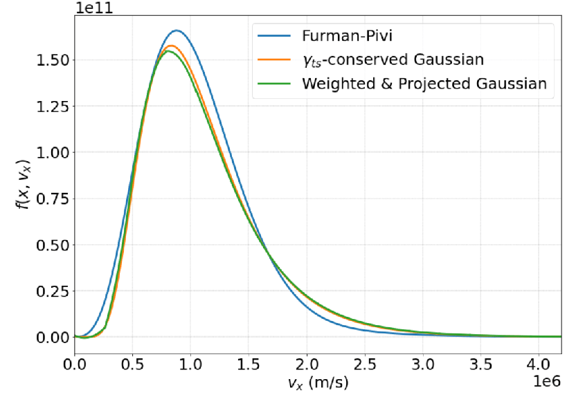
Figure 6: Comparison of exact Furman-Pivi spectrums summed across incoming cells, yield-conserving Gaussian, and simplified Gaussian projected onto the basis. Loss of accuracy is minimal despite the simplifications.

V Discrete Implementation

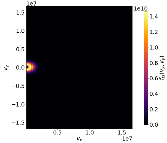
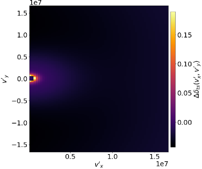
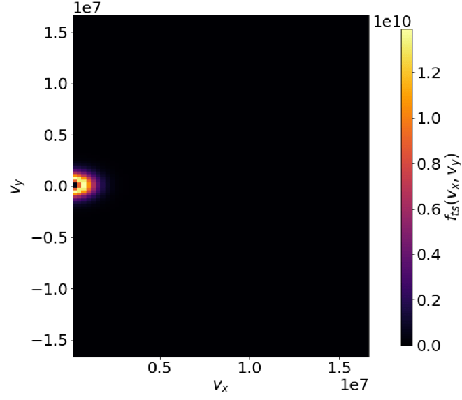
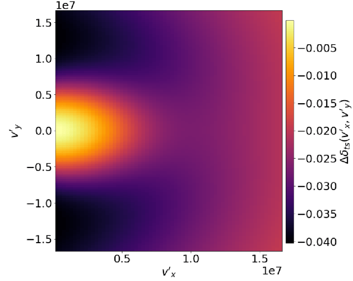
Figure 7: 2V extension of the emission model for the Furman-Pivi theory (top) and Gaussian (bottom). Despite the angular dependence of $\frac{\partial\delta_{ts}}{\partial E}$, the two spectrum distributions are azimuthally uniform (left). Integrating over the Furman-Pivi spectrum to get the yield results in the same error spike at low energy seen in 1V, while the Gaussian has low error throughout the domain (right).

V.1 Emission Spectrum

The implementation of these models on the discrete level requires some modifications. The previous plots were generated from the summation of unique spectrums from hundreds of incoming monoenergetic beams along the impacting distribution. Thus, an immediate necessary simplification is to cut the number of emission spectrums down to one for each cell center velocity. Requiring even each cell to store its own unique emission spectrum can be impractical, however, particularly for multidimensional simulations on large grids. Thus, it is very desirable to consolidate into a single emission spectrum. We take advantage of the fact that cell emission spectrums share a shape, and the observation made earlier that the fitting parameters are not significantly different across the domain for different incoming energies; the major difference lies only in the normalization factor. Therefore, scaling the emitted distribution by the cumulative SEY of the entire incoming distribution using a weighted average should suffice. The weighted average is done using a loop over the velocity space skin cells, the cell center fluxes and the 0th expansion coefficient of the distribution function,

$$\bar{\delta}_{ts}=\frac{\sum_{j=1}^{N_{v}}v_{c}^{j}\hat{f}^{j}_{\alpha,0}\delta_{ts}(v_{c}^{j})}{\sum_{j=1}^{N_{v}}v_{c}^{j}\hat{f}^{j}_{\alpha,0}}.$$ (31)

This effectively weights each value of $\delta$ by its contribution to the total incoming flux. Then, we simply substitute in this value for $\delta_{ts}$ in the calculation for $C$, generating a single, overall normalization factor. The chosen emission spectrum function $f_{ts}$ is projected onto the basis in the initialization of the simulation using the methods described in Section II-B, and scaled each time step by the freshly calculated $C$.

The calculation of $C$ requires us to obtain the flux into the wall, $\Gamma_{\alpha}^{+}$. This flux is most accurately described as the distribution lost to the wall during a time step, or, in numerical terms, the RHS terms of Eq. 3 in the ghost cell, $\frac{\partial f_{h\alpha}^{g}}{\partial t}$. Taking the integrated density of this quantity gives us the total flux,

$$\begin{split}\Gamma_{\alpha}^{+}=\int_{\mathcal{I}}\frac{\partial f^{g+}_{h\alpha}}{\partial t}(\bm{\eta}_{\mathbf{x}},\bm{\eta}_{\mathbf{v}})\mathcal{J}_{\mathbf{x},\mathbf{v}}(\bm{\eta}_{\mathbf{x}},\bm{\eta}_{\mathbf{v}})d\bm{\eta}_{\mathbf{x}}d\bm{\eta}_{\mathbf{v}},\end{split}$$ (32)

where $\mathcal{J}_{\mathbf{x},\mathbf{v}}(\bm{\eta}_{\mathbf{x}},\bm{\eta}_{\mathbf{v}})=\left|\frac{\partial(\mathbf{x},\mathbf{v})}{\partial(\bm{\eta}_{\mathbf{x}},\bm{\eta}_{\mathbf{v}})}\right|$ is the Jacobian matrix transformation from physical to logical space.

The combined steps for calculating the boundary condition are described in Alg. 2, which is inserted into the RK update (see Alg. 1). Each update step after the RHS terms are calculated but before the forward Euler is advanced, $\frac{\partial f}{\partial t}$ in the ghost cell is used to calculate the distribution lost to the wall over the course of a time step (i.e. the flux into the wall). A loop is done over the skin cells to calculate the weighted yield as described by Eq. 31, which is used to calculate the normalization factor. After the time step is advanced, the elastic portion is calculated from the updated skin cell, and both this distribution and the scaled emission spectrum are applied to the ghost cells.

The resulting function is compared to the theoretical Furman-Pivi spectrum, and the yield conserving Gaussian spectrum in Fig. 6. Even with this averaging and discretization, the resultant distribution suffers only minor loss of accuracy.

The methodology outlined here can be extended beyond electron-impact SEE, and the algorithm allows for multiple impact species to be considered. It merely requires an equivalent model to replace the Furman-Pivi model aimed towards ion-impact SEE or whichever desired emission phenomenon.

// Loop over species, calculation of $\frac{\partial f_{hs}}{\partial t}$ VM-FP RHS terms

// Calculate flux into the wall $\Gamma^{+}_{\alpha}$ from RHS terms in ghost cell

$\Gamma^{+}_{\alpha}=$ integratedDensity($\frac{\partial f^{g+,n}_{h\alpha}}{\partial t}$);

// Loop over skin cell phase space into the wall, $\mathcal{X}^{s}$, $\mathcal{V}^{+}$, calculate numerator $w_{1}$ and denominator $w_{2}$ of weighting function

for $i\in\mathcal{X}^{s}$ do

      for $j\in\mathcal{V}_{\alpha}^{+}$ do

            $w^{i}_{1}+=v_{c}^{j}\hat{f}^{ij,n}_{\alpha,0}\delta_{ts}(v_{c}^{j})$;

             $w^{i}_{2}+=v_{c}^{j}\hat{f}^{ij,n}_{\alpha,0}$;

       end for

      $\bar{\delta}^{i}_{ts}=w^{i}_{1}/w^{i}_{2}$;

       // Calculate the normalization factor

       $C^{i}=$ calculateNormalizationFactor($\bar{\delta}^{i}_{ts}$, $\Gamma^{i+}_{\alpha}$);

end for

// Advance with Forward Euler and RK update from $f_{s}^{n}$ to $f_{s}^{n+1}$

// Calculation of elastic backscattering spectrum

$f_{h,e}=$ multiply($\delta_{h,e},f^{s,n+1}_{h\beta}$);

// Accumulate emission spectrums to updated distribution ghost cell

$f^{g,n+1}_{h\beta}=$ accumulate($Cf_{h,ts},f_{h,e}$);

Algorithm 2 Emission spectrum update algorithm

V.2 Elastic Emission

As stated, the elastic boundary condition is the direct scaling of the incoming distribution in the skin cells by some $\delta_{e}$, which is then reflected to become the outgoing distribution in the ghost cells. In the discrete sense, this becomes:

$$f^{g-}_{h\beta}(\mathbf{x},\mathbf{v})=\delta_{he}(\mathbf{v})f^{s+}_{h\beta}(\mathbf{x}^{-},\mathbf{v}^{-}).$$ (33)

Here, the coordinates $\mathbf{x}^{-}$, $\mathbf{v}^{-}$ denote the incoming coordinates being transformed into their outgoing coordinates. In the simplest cases, as touched on in the section on constant yield, $\delta_{e}$ may be taken as a constant across velocity space. For implementations where $\delta_{e}$ is allowed to vary with the incoming energy, it must be implemented as a discrete function. Unlike our implementation of $\delta_{ts}$, this yield is not being used to scale a projected continuous function, and thus cannot be merely evaluated at each cell center and then multiplied by the distribution in that cell. Doing so means multiplying a set of discrete functions by different constant values, which leads to sharper discontinuities in the distribution function at the cell edges and can drive increasing and ultimately fatal numerical noise. Instead, there must be a weak multiplication of the two discrete functions $\delta_{h,e}$ and $f_{h}$,

$$\hat{f}^{g-}_{\beta e}=\int_{\mathcal{I}}\delta_{h,e}(\bm{\eta}_{\mathbf{v}})f^{s+}_{h\beta}(\bm{\eta}^{-}_{\mathbf{x}},\bm{\eta}^{-}_{\mathbf{v}})\psi_{t}(\bm{\eta}_{\mathbf{x}},\bm{\eta}_{\mathbf{v}})d\bm{\eta}_{\mathbf{x}}d\bm{\eta}_{\mathbf{v}}.$$ (34)

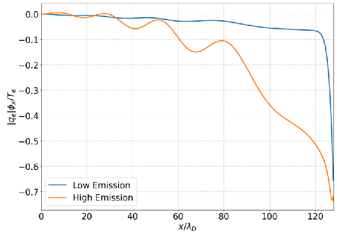
Figure 8: Plot of the potential profiles for the two cases at $t\omega_{pe}=100$. The high emission case is oscillatory due to the rapidly changing sheath dynamics, but a clear non-monotonic potential dip is located at the wall during this phase of the simulation, indicating the presence of the SCL sheath until it collapses by around $t\omega_{pe}=500$ when the yield is driven too low to sustain it. As expected, the low emission case is much smoother and remains classical

VI Discussion

We have demonstrated the basic numerical algorithm for implementation of SEE models into a continuum kinetic boundary condition. The result is a fully energy-dependent emission algorithm that robustly handles the full range of incoming energies, and is applicable for any material for which an SEY curve may be obtained. In this section, we will address the question of how introducing angular effects changes the emission spectrum, and conclude by showing the results of implementing this boundary condition in sheath simulations across a couple different parameter regimes.

VI.1 Angular Dependence of the Emitted Distribution

The plots shown so far have been from emission in a single velocity space dimension. Adding in the second activates an angular dependence in Eq. 21 and the spectrum. The emission spectrum can be assumed to follow a $\cos{\theta}$ angular distribution [28]. However, this does not translate to merely scaling $f_{ts}$ by a factor of $\mu$. Returning to the flux balance of the emitted distribution and incoming beam, Eq. 27 , when we extend it to 2V for $v_{x}$, $v_{y}$, the result is

$$f_{ts}(v_{x},v_{y})=\frac{v^{\prime}_{x}}{v_{x}}\mu(v_{x},v_{y})f_{in}(x=x_{wall},v^{\prime}_{x},v^{\prime}_{y})\frac{m_{e}}{q_{0}}\frac{\partial\delta}{\partial E}\bigg{(}E(v_{x},v_{y}),E^{\prime}(v^{\prime}_{x},v^{\prime}_{y}),\mu^{\prime}(v^{\prime}_{x},v^{\prime}_{y})\bigg{)}dv_{x}dv_{y}.$$ (35)

The solution to the Gaussian spectrum function gained by evaluating Eq. 12 in 2V is

$$C_{G}=\frac{\delta_{ts}\Gamma_{\alpha}^{+}m_{\beta}^{3/2}}{4\sqrt{\pi}(q_{0}E_{0})^{3/2}\tau\exp{(9\tau^{2}/8)}}.$$ (36)

At first glance this introduces a serious issue for our implementation, as Eq. 35 states that the emitted distribution is dependent on the outgoing velocity, something which makes scaling the uniform $f_{ts}$ by a constant $C$ incorrect. However, the dependence on the emitted normal velocity $v_{x}$ in Eq. 35 drops out between the numerator of $\mu$ and the ratio $v^{\prime}_{x}/v_{x}$, meaning that while the particles are emitted in a $\cos{\theta}$ distribution, the cumulative emitted distribution function over a time step is actually uniform with angle. Thus, our Gaussian or Chung-Everhart spectrum approximations for $f_{ts}$ do not need to be scaled by any angular dependence, and no modification to the normalization factor is necessary.

As indicated, the only angular dependence in the normalization factor is the incoming angle for $\delta_{ts}(E^{\prime},\mu^{\prime})$. The Furman-Pivi and Gaussian spectrums calculated from Eq. 35 demonstrating this are shown in Fig. 7, alongside error plots for the resulting $\delta_{ts}$ gained by integrating these spectrums. We see the same error spike that was present in 1V at low energy in the Furman-Pivi plots for the same reason as before. Otherwise, both the Furman-Pivi and Gaussian have very low error in 2V. The same overall algorithm from Alg. 2 remains applicable when extended to multiple dimensions.

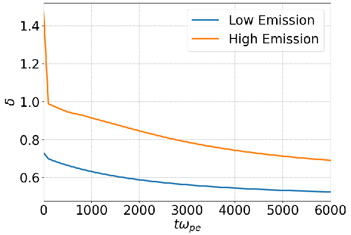
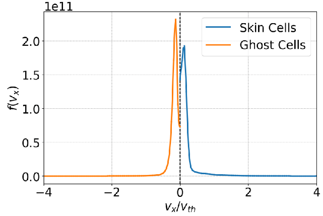
Figure 9: Emission behavior of the two cases. While starting greater than unity, the yield (left plot) quickly drops as a result of decompressional cooling during the sheath formation. It continues to be driven lower with time, eventually causing collapse back to a classical sheath. The right plot of the high emission case at $t\omega_{pe}=100$, which has the impacting distribution on the right, emitted distribution on the left, shows that the SCL is reflecting low energy particles back to the wall while the high energy tail is depleted, causing a spike near zero in the impacting distribution, shifting it towards low energy and driving this downwards trend.

VI.2 Simulations

Test simulations were run to demonstrate the application of these models and verify that we recover the expected sheath behavior when running in the appropriate yield regime. For these simulations, the Gaussian spectrum was used with $E_{0}=1.97$ and $\tau=0.88$. A Maxwellian with $n_{0}=$1.0\text{\times}{10}^{17}\text{\,}\mathrm{m}^{-3}$$ initial distribution was discretized onto a grid spanning $[0,128\lambda_{D}]$ with $N_{x}=1024$ in configuration space, and $[-4v_{t,e},4v_{t,e}]$ and $[-3u_{B},3u_{B}]$ for electrons and ions, respectively, with $N_{v}=128$ in velocity space, where $v_{t,e}=\sqrt{T_{e}/m_{e}}$ is the electron thermal velocity. A mass ratio of $m_{i}/m_{e}=1836$ was used, along with an ion temperature $T_{i}=$2\text{\,}\mathrm{e}\mathrm{V}$$. Two cases were run, a high emission case where the initial electron temperature was $T_{e}=$200\text{\,}\mathrm{e}\mathrm{V}$$, giving an initial yield $\delta_{0}=1.47$, and a low emission case with $T_{e}=$20\text{\,}\mathrm{e}\mathrm{V}$$, $\delta_{0}=0.73$. LBO collisions were utilized, with a mean free path of $\lambda_{mfp}=50\lambda_{D}$, for a few collisions per transit time. Self-species collision frequencies were set to $\nu_{ss}=v_{t,s}/\lambda_{mfp}$, and cross-species to $\nu_{ei}=\nu_{ee}$, $\nu_{ie}=(m_{e}/m_{i})\nu_{ee}$ [33]. Finally, a source term was added to the RHS of Eq. 3 to replenish particle losses to the wall. This was done by scaling the lost ion flux by a linear profile in the presheath and adding equal numbers of electrons and ions back to the simulation,

$$\frac{\Gamma_{i}}{L_{src}}\frac{2(L_{src}-x)}{L_{src}}f_{0,s},\quad 0\leq x\leq L_{src},$$ (37)

where $L_{src}=40\lambda_{D}$ is the source length, and $f_{0,s}$ is the Maxwellian at initial temperature normalized to a density of unity.

If $\delta_{0}$ were held constant, we would expect a classical sheath to form for the low emission case, and ultimately an inverse sheath to form for the high emission case. Fig. 8 shows that, as expected, the low emission case produces a classical sheath, while the high emission case produces a (temporary) space-charge limited sheath. The SCL never transitions to a reverse sheath, instead collapsing to a classical sheath later in time. During the period of SCL development, the high emission case is oscillatory as the emission at the wall rapidly adjusts to match the developing sheath. The profile smooths out as the SCL collapses and the sheath stabilizes. The plot of yield with time in Fig. 9 demonstrates why this is the case, as sheath formation leads to a near-immediate drop in the yield below unity. As the SCL forms, low energy particles emitted from the wall are reflected back to the wall by the potential barrier, leading to a feedback loop of particle accumulation in the distribution at low energy as many of these particles are reemitted in turn due to backscattering. This shifts the distribution towards zero, driving the total yield lower over time as backscattering begins to dominate over the true secondary emission. This combined with the decompressional cooling in the sheath eventually drive the yield below the critical value, leading to the ultimate collapse of the SCL sheath to classical profiles. These classical profiles for both cases do appear to trend towards steady-state at long time scales.

Detailed analysis of these feedback mechanisms and how the space-charge limited and inverse sheath regimes are impacted by the dynamic emission, particularly in comparison to the constant case, will be examined in future work. For now the main focus of these cases is to demonstrate that our results bear up our prediction that yield can be highly dynamic when accounting for fluctuations in the sheath behavior, and that we do indeed recover fundamental sheath behavior (classical, SCL) in corresponding yield regimes. This work presents the first description of a self-consistent, physically-representative model of electron emission from material walls for a range of plasma regimes.

Data Availability Statement

All the simulation results presented in this paper were produced by and are reproducible using the open-source Gkeyll software. Information for obtaining, installing, and running Gkeyll may be found on the documentation site [18]. The input files for the simulations used to produce the results in this paper may be acquired from the repository at https://github.com/ammarhakim/gkyl-paper-inp/tree/master/2023_PSST_ModelSEE.

References

- Birdsall and Langdon [1991] C. Birdsall and A. Langdon, Plasma Physics via Computer Simulation (CRC Press, 1991).
- Cagas et al. [2017] P. Cagas, A. Hakim, J. Juno, and B. Srinivasan, Continuum kinetic and multi-fluid simulations of classical sheaths, Physics of Plasmas 24, 022118 (2017), https://doi.org/10.1063/1.4976544 .
- Cagas [2018] P. Cagas, Continuum kinetic simulations of plasma sheaths and instabilities (2018), arXiv:1809.06368 [physics.plasm-ph] .
- Furman and Pivi [2003] M. Furman and M. T. Pivi, Simulation of secondary electron emission based on a phenomenological probabilistic model, Tech. Rep. (Lawrence Berkeley National Lab.(LBNL), Berkeley, CA (United States), 2003).
- Azzolini et al. [2018] M. Azzolini, M. Angelucci, R. Cimino, R. Larciprete, N. M. Pugno, S. Taioli, and M. Dapor, Secondary electron emission and yield spectra of metals from monte carlo simulations and experiments, Journal of Physics: Condensed Matter 31, 055901 (2018).
- Bohm [1949] D. Bohm, The Characteristics of Electrical Discharges in Magnetic Fields (MacGraw-Hill, New York, 1949).
- Riemann [1991] K. U. Riemann, The bohm criterion and sheath formation, Journal of Physics D: Applied Physics 24, 493 (1991).
- Li et al. [2022] Y. Li, B. Srinivasan, Y. Zhang, and X.-Z. Tang, Bohm criterion of plasma sheaths away from asymptotic limit (2022), arXiv:2201.11191 [physics.plasm-ph] .
- Tang and Guo [2017] X.-Z. Tang and Z. Guo, Bohm criterion and plasma particle/power exhaust to and recycling at the wall, Nuclear Materials and Energy 12, 1342 (2017).
- Hobbs and Wesson [1967] G. D. Hobbs and J. A. Wesson, Heat flow through a langmuir sheath in the presence of electron emission, Plasma Physics 9, 85 (1967).
- Schwager [1993] L. A. Schwager, Effects of secondary and thermionic electron emission on the collector and source sheaths of a finite ion temperature plasma using kinetic theory and numerical simulation, Physics of Fluids 5, 631 (1993).
- Campanell [2013] M. D. Campanell, Negative plasma potential relative to electron-emitting surfaces, Phys. Rev. E 88, 033103 (2013).
- Campanell and Umansky [2016] M. D. Campanell and M. V. Umansky, Strongly emitting surfaces unable to float below plasma potential, Phys. Rev. Lett. 116, 085003 (2016).
- Sheehan et al. [2014] J. P. Sheehan, I. D. Kaganovich, H. Wang, D. Sydorenko, Y. Raitses, and N. Hershkowitz, Effects of emitted electron temperature on the plasma sheath, Physics of Plasmas 21, 063502 (2014), https://doi.org/10.1063/1.4882260 .
- Jensen [2018] K. Jensen, Introduction to the Physics of Electron Emission (John Wiley & Sons, Inc, New Jersey, 2018) pp. 155–161.
- Dougherty [1964] J. P. Dougherty, Model Fokker-Planck Equation for a Plasma and Its Solution, Physics of Fluids 7, 1788 (1964).
- Cockburn and Shu [2001] B. Cockburn and C.-W. Shu, Runge–kutta discontinuous galerkin methods for convection-dominated problems, Journal of Scientific Computing 16, 173 (2001).
- Gkeyll [2023] Gkeyll, (2023), https://gkeyll.readthedocs.io.
- Cagas et al. [2020] P. Cagas, A. Hakim, and B. Srinivasan, Plasma-material boundary conditions for discontinuous galerkin continuum-kinetic simulations, with a focus on secondary electron emission, Journal of Computational Physics 406, 109215 (2020).
- Hakim et al. [2014] A. H. Hakim, G. W. Hammett, and E. L. Shi, On discontinuous galerkin discretizations of second-order derivatives (2014), arXiv:1405.5907 [physics.comp-ph] .
- Juno et al. [2018] J. Juno, A. Hakim, J. TenBarge, E. Shi, and W. Dorland, Discontinuous galerkin algorithms for fully kinetic plasmas, Journal of Computational Physics 353, 110 (2018).
- Hakim et al. [2020] A. Hakim, M. Francisquez, J. Juno, and G. W. Hammett, Conservative discontinuous galerkin schemes for nonlinear dougherty–fokker–planck collision operators, Journal of Plasma Physics 86, 905860403 (2020).
- Juno [2020] J. Juno, A deep dive into the distribution function: Understanding phase space dynamics with continuum vlasov-maxwell simulations (2020), arXiv:2005.13539 [physics.plasm-ph] .
- Hakim and Juno [2020] A. Hakim and J. Juno, Alias-free, matrix-free, and quadrature-free discontinuous galerkin algorithms for (plasma) kinetic equations, in Proceedings of the International Conference for High Performance Computing, Networking, Storage and Analysis (IEEE Press, 2020).
- Scholtz et al. [1996] J. Scholtz, D. Dijkkamp, and R. Schmitz, Secondary electron emission properties, Philips Journal of Research 50, 375 (1996), new Flat, Thin Display Technology.
- Chung and Everhart [1974] M. Chung and T. Everhart, Simple calculation of energy distribution of low‐energy secondary electrons emitted from metals under electron bombardment, Journal of Applied Physics 45, 707 (1974).
- Baglin et al. [2001] V. Baglin, I. Collins, B. Henrist, N. Hilleret, and G. Vorlaufer, A Summary of Main Experimental Results Concerning the Secondary Electron Emission of Copper, Tech. Rep. (CERN, Geneva, 2001) revised version number 1 submitted on 2002-06-24 11:29:13.
- Furman and Pivi [2002] M. A. Furman and M. T. F. Pivi, Probabilistic model for the simulation of secondary electron emission, Phys. Rev. ST Accel. Beams 5, 124404 (2002).
- Larciprete et al. [2013] R. Larciprete, D. R. Grosso, M. Commisso, R. Flammini, and R. Cimino, Secondary electron yield of cu technical surfaces: Dependence on electron irradiation, Phys. Rev. ST Accel. Beams 16, 011002 (2013).
- Cimino et al. [2015] R. Cimino, L. A. Gonzalez, R. Larciprete, A. Di Gaspare, G. Iadarola, and G. Rumolo, Detailed investigation of the low energy secondary electron yield of technical cu and its relevance for the lhc, Phys. Rev. ST Accel. Beams 18, 051002 (2015).
- Cimino et al. [2004] R. Cimino, I. R. Collins, M. A. Furman, M. Pivi, F. Ruggiero, G. Rumolo, and F. Zimmermann, Can low-energy electrons affect high-energy physics accelerators?, Phys. Rev. Lett. 93, 014801 (2004).
- Bronold and Fehske [2015] F. X. Bronold and H. Fehske, Absorption of an electron by a dielectric wall, Physical Review Letters 115, 10.1103/physrevlett.115.225001 (2015).
- Braginskii [1965] S. I. Braginskii, Transport processes in a plasma (1965).