Pointer Networks with Q-Learning for OP Combinatorial Optimization

Abstract

The Orienteering Problem (OP) presents a unique challenge in combinatorial optimization, emphasized by its widespread use in logistics, delivery, and transportation planning. Given the NP-hard nature of OP, obtaining optimal solutions is inherently complex. While Pointer Networks (Ptr-Nets) have exhibited prowess in various combinatorial tasks, their performance in the context of OP leaves room for improvement. Recognizing the potency of Q-learning, especially when paired with deep neural structures, this research unveils the Pointer Q-Network (PQN). This innovative method combines Ptr-Nets and Q-learning, effectively addressing the specific challenges presented by OP. We deeply explore the architecture and efficiency of PQN, showcasing its superior capability in managing OP situations.

1 Introduction

1.1 Motivation

The Orienteering Problem (OP) holds significance in combinatorial optimization, notable for its applications in logistics, sightseeing, and location-based tasks. Its NP-hard nature underscores the difficulty in securing optimal solutions for expansive OP instances. While Ptr-Nets alone or integrated with actor-critic frameworks like Hierarchical RL have been effective for problems like TSP, there’s a noticeable gap when it comes to OP. In such situations, the focused nature of critic-only methods, which center on value estimation, can be particularly advantageous. These approaches can potentially offer more stable learning in environments riddled with sparse rewards or where policy fluctuations might be disruptive. With these considerations, we introduce the Pointer Q-Network (PQN)—a blend of Ptr-Nets and Q-learning. While not crafted exclusively for OP, PQN demonstrates a marked improvement in handling OP tasks compared to the mentioned approaches. The subsequent sections will detail PQN’s architecture and its proficiency in managing the intricacies of OP.

1.2 Contribution

Amid rising real-world challenges, scalable methods that maintain solution quality are essential. Enter Pointer Networks (Ptr-Nets), which revolutionized sequence-to-sequence modeling for combinatorial problems using deep learning [Vinyals et al., 2015]. Concurrently, Q-learning’s capabilities, amplified by deep architectures in Deep Q-Networks (DQN) [Mnih et al., 2015], heralded new avenues for innovation. Innovations like S2V-DQN and ECO-DQN blended graph embeddings with reinforcement learning for enhanced combinatorial optimization. Furthermore, merging Ptr-Nets with Hierarchical RL [Qiang Ma et al. 2019] showcased their potency in this domain. Collectively, these advancements highlight deep learning’s adaptability and the continuous evolution in optimization techniques.

2 Background and problem formulation

In this section, we delve into the technical intricacies of the Orienteering Problem (OP) and investigate its interplay with Markov Decision Processes (MDP). A precise and adept integration between these two paradigms is pivotal, as it establishes the sequence that determines affinity with the proposed system, PQN.

2.1 Orienteering Problem (OP)

Definitions The OP is a combinatorial optimization problem which entails identifying a route that initiates from a specified starting vertex, potentially traverses through a subset of accessible vertices, and aims to maximize the accrued prize, all while not exceeding a given budget (or time constraint). The problem can be described formally using the tuple $\mathcal{O}=\langle\mathcal{V},\mathcal{E},p,c,B,s,t\rangle$, where $\mathcal{V}$ signifies the set of vertices $v$, which includes the starting and potential end points; $\mathcal{E}$ represents the set of edges $e$ or connections between the vertices; $p:\mathcal{V}\rightarrow\mathbb{R}^{+}$ is the prize function that associates each vertex with a non-negative prize value; $c:\mathcal{E}\rightarrow\mathbb{R}^{+}$ stands for the cost function, attributing a non-negative cost to each edge in $\mathcal{E}$; $B$ is the set ceiling for the route in terms of budget or time; $s$ (optional) is the designated onset vertex; and $t$ (optional) can indicate a specific ending vertex, if the route is intended to conclude at a distinct point.

For our solution, we’ll define the decision variables as follows: $x_{ij}$ is a binary variable that is 1 if edge $(i,j)$ is included in the chosen route and 0 otherwise; $u_{v}$ is an auxiliary variable indicating the sequence or position of the vertex $v$ in the route.

Our objective function, which gauges the merit of a solution via the rewards of various routes, is:

$$\max\sum_{v\in\mathcal{V}}p_{v}\cdot\delta_{v}$$ (1)

Where $\delta_{v}$ is 1 if vertex $v$ is visited and 0 otherwise.

Constraints The following set of constraints is crucial to guarantee that our solutions are viable for OP:

• Route originates at vertex $s$:

  $$\sum_{j\in\mathcal{V}}x_{sj}=1$$ (2)

• Flow conservation:

  $$\sum_{i\in\mathcal{V}}x_{iv}-\sum_{j\in\mathcal{V}}x_{vj}=0,\quad\forall v\in\mathcal{V}$$ (3)

• Travel cost must not surpass the designated maximum:

  $$\sum_{i\in\mathcal{V}}\sum_{j\in\mathcal{V}}c_{ij}\cdot x_{ij}\leq B$$ (4)

• Subtour elimination:

  $$u_{i}-u_{j}+|\mathcal{V}|\cdot x_{ij}\leq|\mathcal{V}|-1,\quad\forall(i,j)\in\mathcal{E},i\neq j$$ (5)

  $$1\leq u_{v}\leq|\mathcal{V}|,\quad\forall v\in\mathcal{V}$$ (6)

• Avoid revisiting a vertex:

  $$\sum_{i\in\mathcal{V}}x_{iv}+\sum_{j\in\mathcal{V}}x_{vj}\leq 2,\quad\forall v\in\mathcal{V}$$ (7)

• Optionally, not concluding at the starting vertex:

  $$v_{\text{end}}\neq v_{\text{start}}$$ (8)

2.2 Integrating OP with MDP

In a similar vein to the structure2vec (S2V) method [Khalil et al. 2018], we embed a given graph into a vector. Instead of crafting a recursive network directly, we utilize an MDP. Our representation is meticulously constructed, allowing for later approximation of Q-values via a hybrid network. Details of this will be elaborated upon in the sections to follow.

MDP The reinforcement learning agent’s playground is an environment defined as a Markov Decision Process. In our scenario, this MDP is given by the tuple $\mathcal{M}=\langle\mathcal{S},\mathcal{A},P,R,\gamma\rangle$, where $\mathcal{S}$ embodies the state space; $\mathcal{A}$ is the action space; $P:\mathcal{S}\times\mathcal{A}\times\mathcal{S}\mapsto[0,1]$ characterizes the state transition probability function; $R:\mathcal{S}\mapsto\mathbb{R}$ is the reward function; and $\gamma\in[0,1]$ signifies the discount factor, which determines the present value of future rewards. Furthermore, the episode tuple, $E=\langle s,a,r,s^{\prime}\rangle$, will prove crucial in later parts of the text, especially when illustrating the model’s training regimen.

Embedding of OP into an MDP Drawing parallels from graph embedding and sequence2vec, it becomes essential to recast the graph into a familiar construct like an MDP. This reshaping paves the way for the agent’s seamless interactions, empowering it to draw lessons effectively from every interaction within the organized environment. The state in our defined MDP encapsulates the ongoing status of the evolving route. The state is delineated as $s=\langle\mathcal{R},B,\mathbf{X}\rangle$, where $\mathcal{R}$ stands for the ongoing route, and the last vertex in $\mathcal{R}$ signifies the present vertex $v_{\text{current}}$. The term $B$ denotes the outstanding budget, while $\mathbf{X}$ is a binary indicator vector. Here, $X_{i}=1$ if vertex $v_{i}$ is already visited and $0$ otherwise. Every action $a$ in our MDP is analogous to choosing a vertex $v$. Formally, the action space $\mathcal{A}$ is captured as $\mathcal{A}(s)=\{a:v|v\in V\land X_{v}=0\}$, ensuring only unvisited vertices emerge as valid actions for any existing state. Transition dynamics encapsulate the potential of migrating from a state to another in light of a particular action. Given OP’s deterministic characteristic, our transitions are deterministic. Thus, $P(s^{\prime}|s,a)=1$ if a new state emerges by picking a vertex, and $P(s^{\prime}|s,a)=0$ otherwise. The reward function gauges the gain from executing an action from a particular state to reach a new one. The reward is deduced from the prize of the accessed vertex, and can be mathematically portrayed as $R(s,a,s^{\prime})=p_{a}$, where $p_{a}$ is the prize associated with vertex $a$. Embedding the OP into MDP ensures a systematic framework for our problem, enabling its resolution via reinforcement learning techniques.

3 Proposed approach

In the sections ahead, we will delve into the intricacies of constructing the PQN system. We aim to illuminate the synergistic blend of Ptr-Nets and Q-learning function approximation, furnishing comprehensive explanations complemented by practical model visualizations.

3.1 Critic-Only Reinforcement Learning

Reinforcement learning (RL) techniques are primarily divided into two main categories: Actor-only and Critic-only methods. The Actor-only approach has seen the application of Ptr-Nets (in combinatorial optimization landscapes) by leveraging the capabilities of Hierarchical Reinforcement Learning [Qiang Ma et al. 2019], directly deriving and optimizing the policy. Our research is centered on the Critic-only methods, which revolve around the concepts of Value and Q-value.

At its core, the Value function, $V^{\pi}(s)$, represents the expected reward when starting in state $s$ and following a specific policy $\pi$. In contrast, the Q-value function $Q^{\pi}(s,a)$, builds upon this concept by considering the action taken. The underlying principle of Critic-only methods is based on the Bellman equation Definitions and proofs.

For the purpose of integration with the Ptr-Net framework, it is imperative to delineate the primary strengths and shortcomings of both proposed models. Understanding these nuances is pivotal, as they will influence later deepened design decisions.

Tabular Q-Learning This is indeed a model-free reinforcement learning technique that stores Q-values for every state-action pair in a straightforward table. It employs simplicity, iteratively updating Q-values using the Bellman equation. The Temporal Difference (TD) error, $\delta$, represents the gap between the newly observed Q-value and the existing estimate. Specifically, $\delta=Q(s^{\prime},a^{\prime})-Q(s,a)$. By continuously refining Q-values based on this TD error, tabular Q-learning is guaranteed to converge to the optimal policy in deterministic settings Definitions and proofs.

Strengths

• Transparency: The tabular approach offers a clear and interpretable representation of Q-values.

• Convergence: As previously mentioned, given enough time and a suitable policy, tabular Q-learning is guaranteed to converge to the optimal Q-values.

• Simplicity: Without the complexities of neural networks, it’s straightforward to implement and understand.

Weaknesses

• Scalability: The method struggles with large state and action spaces due to the need for a table entry for each state-action pair.

• Generalization: Unlike DQNs, the tabular method cannot generalize across states. It requires explicit exploration of each state-action pair for learning.

Deep Q-Networks DQNs emblematically exemplify the confluence of RL and deep learning (DL). Within the architecture of a DQN, each layer possesses its distinctive weights that undergo training within the primary training loop. Serving as function approximators, DQNs eclipse the traditional practice of storing Q-values in tabular form. A salient component of the DQN framework is the target network. Periodically, this network assimilates the Q-values from the primary DQN to compute the target Q-value. Consequently, the Temporal Difference (TD) error $\delta$ emerges as the difference between this target Q-value and the Q-value derived from the optimal policy, in this way $\delta=Q^{\text{target}}(s,a)-Q^{\pi}(s,a)$. We refresh Q-values iterating the update rule, which indeed makes use of $\delta$ Definitions and proofs.

Strengths

• Scalability: DQNs can manage high-dimensional state spaces, making them apt for complex problems.

• Generalization: They can generalize across states, meaning they don’t need to see every state to make reasonable predictions.

• Stability: With techniques like experience replay and target networks, DQNs address the inherent instability of neural networks in reinforcement learning.

Weaknesses

• Training Complexity: DQNs require significant computational resources and time.

• Hyperparameter Sensitivity: The performance of DQNs can be sensitive to the choice of hyperparameters.

• Overestimation: They have a known tendency to overestimate Q-values.

3.2 Merging Pointer Networks with Q-learning for OP

Overview Pointer Networks (Ptr-Nets), developed by [Vinyals et al. 2015], represent an advancement from traditional sequence-to-sequence models as they adeptly handle varying sequence lengths. Ptr-Nets generate variable-length outputs by referencing positions within the input sequence. Their ability to form sequences based on the importance of each element in the input makes them especially suitable for optimization problems where the length of the optimal solution may vary.

Ptr-Nets have showcased their prowess in handling combinatorial optimization tasks like the Travelling Salesman Problem (TSP). However, in tasks such as OPs, where the sequence length isn’t fixed and the need of capturing relationships between nodes (reward-wise) is imperative, performance drops are noticeable. Recognizing the complexities of such optimization problems, we suggest blending the deterministic vertex selection of Ptr-Nets with the probabilistic Q-value approximation of Q-Learning methods. Instead of exclusively highlighting a single vertex, the Ptr-Net provides a permutation, spotlighting the top $\lambda\in[1,|\mathcal{V}|]$ vertices based on attention scores. Q-Learning then evaluates the Q-values for each state-action combination, leading to the optimal action’s selection and consequently building the optimal route $\pi^{*}$ until the budget is finished.

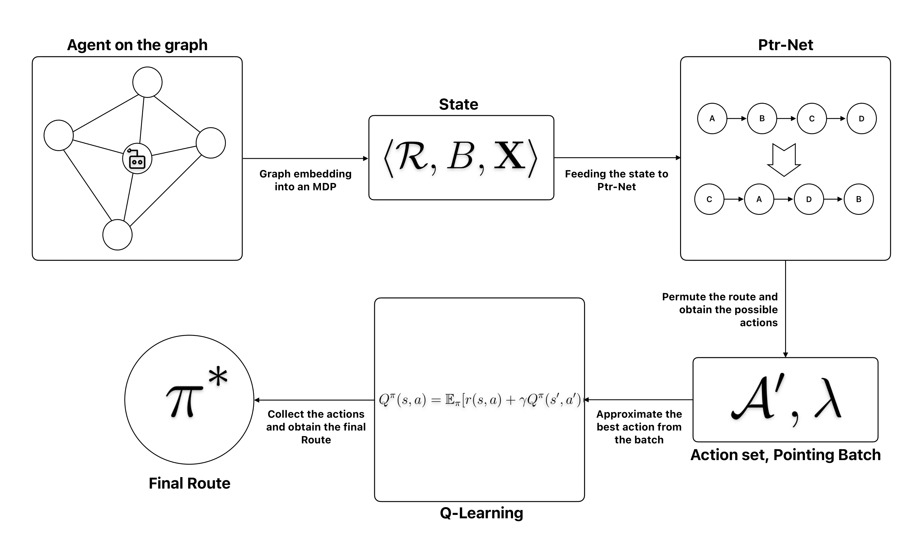
Figure 1: PQN procedure schematization

Pointing Batch Dynamics Introducing the concept of ‘pointing batch‘ denoted by $\lambda\in\mathbb{Z^{+}}$ (which could also take positive real values in continuous contexts), we define the number of vertices the Ptr-Net concentrates on during each selection phase. This allows Q-learning to evaluate these potential actions based on expected outcomes. Depending on the value of $\lambda$, various scenarios emerge:

• $\lambda=1$, the system would merely replicate the traditional approach of pointing to the single most favorable vertex. While this might be computationally efficient, it might not fully harness the capabilities of the Ptr-Net, potentially leaving out other vertices that could be nearly as favorable or even more favorable in certain situations.

• $\lambda\rightarrow 1$: As $\lambda$ leans closer to 1, the problem becomes more discrete and deterministic, but the final policy $\pi$ will likely be suboptimal ($\pi^{-}$). Given $a=v_{\text{unvisited}}$, we can symbolically state that:

  $$\lim_{\lambda\rightarrow 1}\bigg{\{}a_{j}^{-}:\arg\max_{a^{\prime}}\sum_{a^{\prime}\in\mathcal{A^{\prime}}}Q^{\pi}(s,a^{\prime})\bigg{\}}^{L}_{j=1}=\pi^{-}$$ (9)

  where $a^{\prime}=\sum_{i=1}^{\lambda}\arg\max_{i}P(c_{i}|\mathcal{V}_{\text{unvisited}},R)e_{i}$, $L$ is the final route length, $e\in\{0,1\}^{\lambda}$ the canonical basis. In such cases, tabular Q-learning is better suited. Tabular Q-learning works well when the action and state spaces are relatively small, allowing for a more exhaustive exploration of the state-action pairs.

• $\lambda\rightarrow\mathcal{V}$: As $\lambda$ approaches the size of $\mathcal{V}$, the action space becomes broader and more complex. Although the effort of calculation grows significantly, we should point out that the resulting final route in this case will more likely converge to the optimal one ($\pi^{*}$):

  $$\lim_{\lambda\rightarrow|\mathcal{V}|}\bigg{\{}a_{j}^{*}:\arg\max_{a^{\prime}}\sum_{a^{\prime}\in\mathcal{A^{\prime}}}Q^{\pi}(s,a^{\prime})\bigg{\}}^{L}_{j=1}=\pi^{*}$$ (10)

  DQNs are apt for such situations, since they can handle large action spaces effectively.

• $\lambda=|\mathcal{V}|$, the Ptr-Net would consider every possible vertex, rendering the action space vast and computationally challenging to handle in the Q-values estimation process by the DQN subsequently. While this approach ensures a comprehensive assessment of all vertices, it becomes computationally expensive and may introduce redundancy.

Building PQN The Ptr-Net design is split into an encoder $e$ and a decoder $d$. The encoder converts the input sequence into hidden states, while the decoder uses these hidden states to construct the output sequence. To elucidate further, consider an input sequence $\{s_{1},s_{2},\dots,s_{N}\}$. An RNN updates its hidden state $h$ iteratively, encapsulating the input sequence’s representation:

$$h_{i}=\text{tanh}(W_{e}h^{i-1}_{e,v}+W_{d}s_{i}+b_{h})$$ (11)

Here $W$ and $b$ are learnable weights.

For each vertex in the set of unvisited vertices, the encoder generates a corresponding hidden state $h_{e,v}^{i}$.

$$h_{e,v}^{i}=\text{RNN}_{\text{encoder}}(v)\quad\forall v\in\mathcal{V}_{\text{unvisited}}$$ (12)

For each decoding step $t$, the decoder leverages attention over the encoder’s hidden states to derive its hidden state

$$h_{d}^{t}=\text{RNN}_{\text{decoder}}(h_{d}^{t-1},c^{t})$$ (13)

The attention mechanism computes a context vector $c^{t}$:

$$c^{t}=\sum_{v}\alpha^{t}_{v}h_{e,v}^{i}$$ (14)

With attention weights derived from:

$$\alpha^{t}_{v}=\frac{\exp(e^{t}_{v})}{\sum_{v^{\prime}}\exp(e^{t}_{v^{\prime}})}$$ (15)

Here $e$ symbolizes the attention energy, which is no less than a ‘raw attention score‘, computed as follows:

$$e^{t}_{v}=(h_{t-1}^{d})^{T}\cdot h_{i}^{e,v}$$ (16)

The interplay of the context vector and the current decoder state determines the probability distribution over potential actions:

$$P(c_{i}|\mathcal{V}_{\text{unvisited}},\mathcal{R})=\text{softmax}(f(h_{d}^{t},c^{t}))$$ (17)

We employ a feed-forward neural network $f$ in the attention system as it efficiently captures the non-linear relationships and interactions between the decoder state and the context, aiding in generating precise attention scores. The set of subsequent vertex actions, $\mathcal{A}^{\prime}$, is inferred from this distribution:

$$\mathcal{A}^{\prime}=\{a_{i}:\arg\max_{i}P(c_{i}|\mathcal{V}_{\text{unvisited}},R)\}_{i=1}^{\lambda}$$ (18)

Where $\arg\max_{i}$ retrieves the indices corresponding to the top $\lambda$ values of the conditional probabilities, striking a balance between computational efficiency and decision-making richness.

To finalize the process, after obtaining the set of top actions $\mathcal{A}^{\prime}$ from the Ptr-Net, Q-learning approximates the expected return for each action in $\mathcal{A}^{\prime}$, given the current state. Formally, the Q-value for each action $a_{i}$ in $\mathcal{A}^{\prime}$ is given by:

$$Q(s,a_{i})=R(s^{\prime},a_{i},s)+\gamma\max_{a^{\prime}\in\mathcal{A}^{\prime}}Q(s^{\prime},a^{\prime})$$ (19)

Here, $R(s^{\prime},a_{i},s)$ is the expected reward when taking action $a_{i}$ in state $s$ and transitioning to state $s^{\prime}$. The term $\max_{a^{\prime}\in\mathcal{A}^{\prime}}Q(s^{\prime},a^{\prime})$ denotes the maximum Q-value over all potential subsequent actions in $\mathcal{A}^{\prime}$, reflecting the agent’s future value estimation.

From this set of Q-values, the action $a^{*}$ with the highest Q-value is selected as the optimal action:

$$a^{*}=\arg\max_{a_{i}\in\mathcal{A}^{\prime}}Q(s,a_{i})$$ (20)

Policy retrieval post termination Upon reaching the termination condition, the agent has traversed a series of actions that form a tentative route, potentially optimal. It is now essential to extract this policy sequence, represented by $\pi^{*}$, to evaluate its performance concerning the problem’s constraints and objectives. The derived policy should not only conform to the budgetary constraints but also maximize the accrued rewards throughout the episode. Retrieving the policy can be mathematically formulated as:

$$\pi^{*}=\{a_{j}^{*}\}_{j=1}^{L}\quad\text{where}\quad L=\text{dim}(\pi^{*})\quad\text{and}\quad\sum_{j=1}^{L}c_{a_{j}^{*}}\leq B$$

In the above expression, $c_{a_{j}^{*}}$ represents the cost associated with action $a_{j}^{*}$. The total cost of the derived policy $\pi^{*}$ should not exceed the available budget $B$. This retrieval process ensures that the extracted policy is both feasible and aligns with the agent’s learning over the episode.

Addressing challenges The Orienteering Problem (OP) requires a delicate balance between cost minimization and reward maximization within a set budget, a scenario where Ptr-Nets can sometimes fall short, especially when compared to their performance in problems like the TSP. The intricacies of OP can lead Ptr-Nets to favor one objective over the other, potentially neglecting rewarding paths in favor of immediate cost savings.

This is where the integration of Q-learning becomes crucial. With its inherent capability to recognize and prioritize routes with better future rewards, Q-learning offers a more holistic view. When coupled with Ptr-Nets, this combination aids in capturing both immediate and long-term benefits. Adjusting the pointing batch $\lambda$ further refines the process, allowing for optimal scaling of computations based on the specific complexities of the problem at hand.

The resulting Pointer Q-Networks (PQNs) effectively bridge the gap in Ptr-Nets’ approach to OP. While Ptr-Nets point to promising actions in the immediate state, Q-learning evaluates their future implications in terms of both cost and rewards. In increasingly intricate OP scenarios, PQNs offer solutions that seamlessly merge computational efficiency with a balanced consideration of costs and rewards.

Algorithm 1 PQN Algorithm

0:  Input sequence $\{s_{1},s_{2},\dots,s_{N}\}$

0:  Pointing batch size $\lambda$

1:  Initialize Pointer Network (Ptr-Net) with weights $\theta$

2:  Initialize Q-function with weights $\phi$

3:  while episode not terminated do

4:     Encode input sequence using Ptr-Net encoder to get hidden states $h_{e,v}^{i}$

5:     for each decoding step $t$ do

6:        Calculate attention scores and context vector $c^{t}$

7:        Decode using context vector to get $h_{d}^{t}$

8:        Calculate action probabilities $P(c_{i}|\mathcal{V}_{\text{unvisited}},\mathcal{R})$

9:        Select top $\lambda$ actions as $\mathcal{A}^{\prime}$

10:        for each action $a_{i}$ in $\mathcal{A}^{\prime}$ do

11:           Compute Q-value $Q(s,a_{i})$ using current episode $E$

12:        end for

13:        Select optimal action $a^{*}$ with highest Q-value

14:        Update the state based on chosen action

15:     end for

16:     Update Ptr-Net and Q-function weights using respective losses

17:  end while

4 Experiment

Our experiment focuses primarily on comparing the performances of Ptr-Net and PQN in extracting the optimal route based on cumulative reward, while considering various evaluation metrics.

4.1 Setup and Hyperparameters

We conducted experiments in two different settings, denoted as $\mathcal{O}_{20}$ and $\mathcal{O}_{50}$, each with train, evaluation, and test instances. In $\mathcal{O}_{20}$, we set $\mathcal{V}=20$, $\mathcal{E}=190$, and other parameters as $p,c,B,s=0$. In $\mathcal{O}_{50}$, we increased the complexity with $\mathcal{V}=50$, $\mathcal{E}=1225$, and the same other parameters.

In both settings, the graphs are fully connected, resembling real-world scenarios. The prize values $p$ are randomly chosen from the interval [0, 15], while the cost values $c$ range from 0 to 10. The budget $B$ is calculated as $B=\frac{\mathcal{V}}{4}(\langle p\rangle-\langle c\rangle)$, where $\langle p\rangle$ and $\langle c\rangle$ are the average prizes and costs, respectively. We set the sequence length $L_{s}$ equal to $|\mathcal{V}|$, reflecting the number of vertices. The termination node $t$ remains undefined.

Both algorithms operate on the same graph to eliminate potential biases. The aim is to study the model’s decision-making process within budget constraints.

The hyperparameters include:

• $L_{s}$ (sequence length) = $|\mathcal{V}|$

• RNN = LSTM Definitions and proofs

• $H$ (hidden layer size) = 128

• $\lambda$ (pointing batch) = $\frac{L_{s}}{2}$

• $O_{s}$ (output size) = $L_{s}$, but varies due to the satisfaction of termination conditions

• $\eta$ (learning rate) = $10^{-3}$

• Episodes = 20 for $\mathcal{V}=20$ and 50 for $\mathcal{V}=50$

4.2 Losses

In our experimental setup, we utilize distinct loss functions tailored to the specific learning mechanisms of the Pointer Q-Network (PQN) and the Pointer Network (Ptr-Net).

For PQN, the loss function is derived from the standard Q-learning Mean Squared Error (MSE) loss $J$, which originates from the Bellman equation:

$$J(\delta)=\sum_{a^{\prime}}\delta^{2}=\sum_{a^{\prime}}\left(Q(s,a)-\left(r+\gamma\max_{a^{\prime}}Q(s,a^{\prime})\right)\right)^{2}$$ (21)

Here, $\delta$ signifies the temporal difference, capturing the discrepancy between the current Q-value estimate $Q(s,a)$ and the expected return $r+\gamma\max_{a^{\prime}}Q(s,a^{\prime})$. PQN’s loss formulation directly aligns with the Q-learning framework, optimizing the Q-values through the minimization of this MSE loss.

In contrast, Ptr-Net employs a different loss function based on Cross-Entropy (CE) likelihood $l$ of the computed probabilities. The CE loss, $l(P||Q)$, is computed as follows:

$$l(P||Q)=-\sum_{i=1}^{N}\sum_{j=1}^{L_{s}}q_{ij}\log(p_{ij})$$ (22)

Here, $P$ and $Q$ represent the probability distributions for the action selection. $P$ is the model’s prediction, and $Q$ is the ground truth distribution. Ptr-Net’s loss function quantifies the dissimilarity between the predicted action probabilities and the actual action distributions.

It is essential to note that these loss functions are not directly comparable due to their inherent differences. While PQN’s loss function aligns with Q-learning principles and focuses on Q-value optimization, Ptr-Net’s loss centers around probability distribution matching. Using the CE loss for PQN backpropagation might not be suitable, as it does not fully capture the essence of its learning process, which involves comprehensive Q-value computation. These distinct loss functions reflect the diverse learning strategies and objectives of PQN and Ptr-Net in addressing the Orienteering Problem.

4.3 Comparison Metrics

To assess and compare the models, we utilize several metrics, including:

• Cumulative reward $\mathbf{R}=\sum_{k}R_{k}$, where $k$ is a step

• Average loss $\langle l\rangle$ (average CE loss), $\langle J\rangle$ (average Q-MSE loss)

• Convergence speed $t$ expressed in seconds

• Action-selection distribution $\pi$ (indicating action preferences for both models)

4.4 Results and Discussion

We will now present the results of our experiments and provide a comprehensive discussion of the outcomes.

Cumulative Reward

• For $\mathcal{O}_{20}$, Ptr-Net achieved a cumulative reward of $\mathbf{R}=12$ after training and fine-tuning during evaluation, while PQN attained a cumulative reward of $\mathbf{R}=21$.

• For $\mathcal{O}_{50}$, Ptr-Net achieved a cumulative reward of $\mathbf{R}=40$ after training and fine-tuning during evaluation, while PQN attained a cumulative reward of $\mathbf{R}=68$.

The cumulative reward ($\mathbf{R}$) serves as a critical metric to evaluate the performance of Ptr-Net and PQN in solving the Orienteering Problem ($\mathcal{O}$). These results indicate that PQN exhibits a more effective decision-making process, resulting in higher cumulative rewards. A closer examination of action sequences reveals an interesting pattern. Ptr-Net tends to select consecutive nodes, possibly due to its limited ability to explore non-sequential but rewarding paths. In contrast, PQN shows a less greedy approach, recognizing the potential benefits of visiting non-sequential nodes and ultimately achieving higher cumulative rewards.

Average Loss

In our experiments, we observed distinct patterns in the average loss values between Ptr-Net and PQN:

• For $\mathcal{O}_{20}$, Ptr-Net exhibited an average loss of $\langle l\rangle=10.0924$, while PQN encountered an average loss of $\langle J\rangle=59.3423$.

• In the context of $\mathcal{O}_{50}$, Ptr-Net recorded an average loss of $\langle l\rangle=32.2944$, whereas PQN grappled with an average loss of $\langle J\rangle=132.1646$.

It is important to note that, in general, PQN’s loss might take more time to stabilize compared to Ptr-Net. With the same number of episodes, Ptr-Net exhibited quicker convergence to a stable loss value, indicating its ability to adjust rapidly to the given problem settings. However, it is crucial to acknowledge that the speed of convergence in loss values does not necessarily correlate with the effectiveness of a model’s learning strategy. Ptr-Net’s relatively quicker stabilization does not imply that it effectively captures the intricate relationships between nodes within the OP. It may optimize its policy more rapidly but potentially overlook essential nuances in the problem’s structure. Conversely, PQN’s longer stabilization suggests a more deliberate learning process, where the model takes the time to explore various action sequences and evaluate their long-term implications.

Convergence Speed

• For $\mathcal{O}_{20}$, Ptr-Net took $t=13.83s$ to converge, while PQN required $t=40.01s$ for convergence.

• For $\mathcal{O}_{50}$, Ptr-Net took $t=114.37s$ to converge, whereas PQN exhibited a longer convergence time of $t=483.32s$.

This discrepancy in convergence speed can be attributed to the time complexity $\mathbf{O}$ of each approach. Ptr-Net maintains a relatively lower time complexity due to its direct modeling of the policy using the pointing mechanism. In contrast, PQN, which integrates Ptr-Net with Q-learning, inherits the time complexity of both components, resulting in longer convergence times (as deepened in the previous point).

Action-Selection Distribution

• For $\mathcal{O}_{20}$, Ptr-Net often favored sequential actions, indicating a preference for deterministic path selection. In contrast, PQN demonstrated a more diverse approach, exploring non-sequential paths strategically.

• For $\mathcal{O}_{50}$, Ptr-Net continued to favor sequential actions, maintaining its deterministic pattern. PQN, however, retained its preference for non-sequential actions, showcasing its adaptability to complex scenarios.

In our experiment, Ptr-Net and PQN exhibited distinct action-selection preferences when solving the OP. Ptr-Net displays a bias toward sequential actions, often favoring choices that follow a specific order, even in intricate scenarios. In contrast, PQN maintains a preference for actions that underscores its capacity to explore non-sequential nodes. The action sequences from PQN emphasize its tendency to select paths involving non-consecutive nodes. This inclination toward diverse action selection reveals PQN’s robust adaptability to complex OP settings, where sequential decisions may not always lead to the most rewarding solutions.

We can formalize these concepts using the entropy of the distributions Definitions and proofs

$$H(\pi_{\text{Ptr-Net}})<H(\pi_{\text{PQN}})$$

The inequality then reflects the greater diversity and non-sequential nature of action selections in PQN compared to Ptr-Net.

	$\pi_{\text{Ptr-Net}}$	$\pi_{\text{PQN}}$
$\mathcal{O}_{20}$	{16→17→18→19}	{1→3→4→5}
$\mathcal{O}_{50}$	{0→1→2→3→4→5→6→7→8}	{31→30→13→8→39→38→37→36→35}

Table 1: Comparison of the obtained action sequences $\pi$ from both models

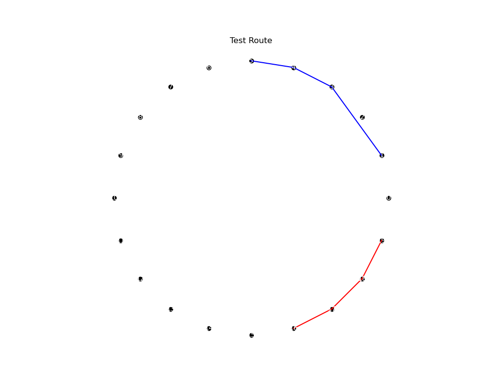
(a) $\mathcal{O}_{20}$

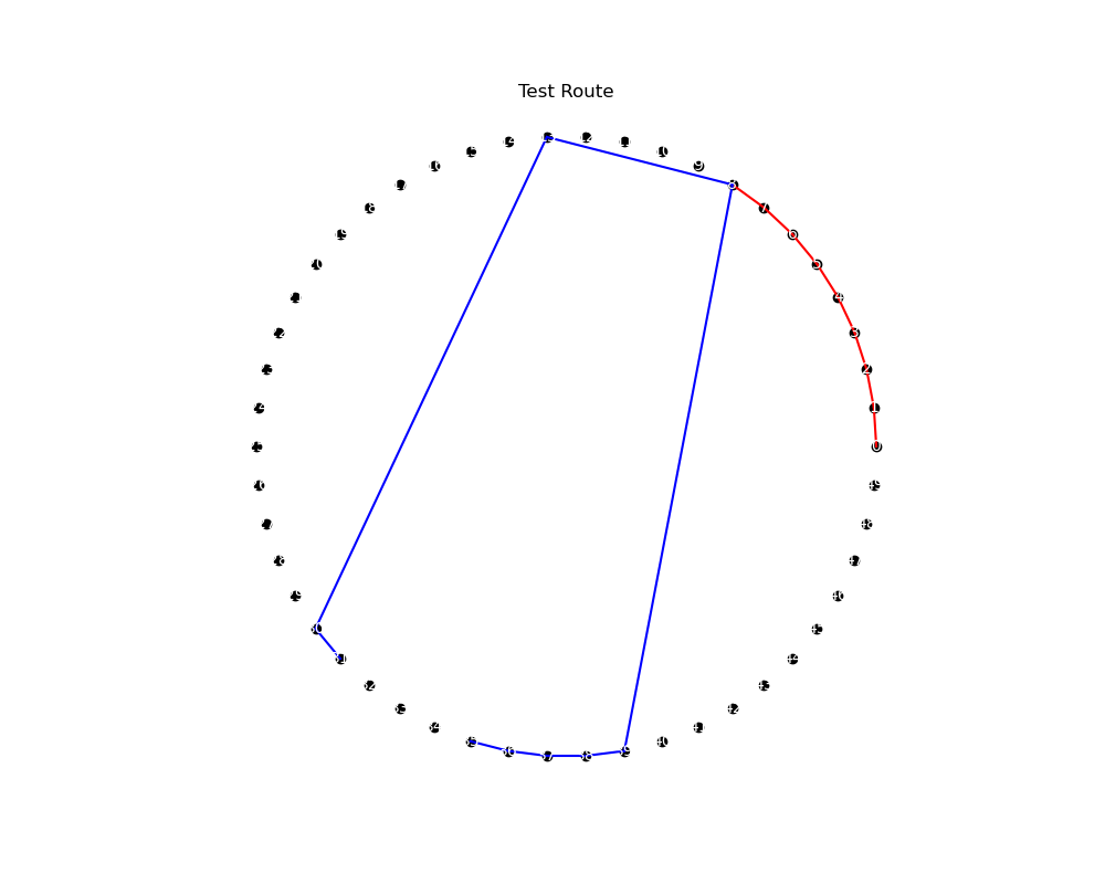
(b) $\mathcal{O}_{50}$

Figure 2: Visualization of the retrieved action sequences $\pi$, Ptr-Net (in red), PQN (in blue)

5 Conclusions

In this paper, we introduced the Pointer Q-Network (PQN) as a novel approach to addressing the Orienteering Problem (OP), a challenging problem in combinatorial optimization with applications in logistics, sightseeing, and location-based tasks. While Pointer Networks (Ptr-Nets) and related methods have shown success in other combinatorial optimization tasks like the Traveling Salesman Problem (TSP), their performance in the context of OP left room for improvement.

PQN merges Pointer Networks with Q-learning to create a new approach to OP. We have demonstrated the advantages of PQN over traditional Ptr-Nets in solving OP instances. Our experimental results show that PQN outperforms Ptr-Net in terms of cumulative rewards, indicating a more effective decision-making process. PQN’s preference for non-sequential actions highlights its adaptability to complex OP scenarios, where sequential decision-making might not always lead to optimal solutions.

The use of Q-learning within the PQN framework helps address the challenges associated with OP. By considering both immediate rewards and long-term benefits, PQN offers a more holistic approach to solving the problem. The choice of the pointing batch parameter $\lambda$ further allows for the fine-tuning of the algorithm’s behavior based on the complexity of the specific problem.

However, it’s important to acknowledge that PQN comes with a trade-off, which is the longer convergence time compared to Ptr-Net. This is due to the integration of two distinct learning processes, pointing mechanisms, and Q-value approximations. The choice between Ptr-Net and PQN should depend on the specific requirements of the problem, where Ptr-Net might be preferred for quicker convergence, while PQN is the better choice for more complex OP scenarios.

In conclusion, the introduced PQNs represent a significant advancement in addressing the Orienteering Problem. PQNs bridge the gap in Ptr-Nets’ approach to OP by offering a balance between computational efficiency and a thorough consideration of costs and rewards. This research opens up exciting avenues for the use of reinforcement learning techniques in solving complex combinatorial optimization problems with budget constraints, benefiting industries such as logistics and tourism.

The continued exploration of PQN’s potential and further research into fine-tuning its parameters to optimize its performance in various OP scenarios are promising areas for future work.

Definitions and proofs

Definition: Values and Q-Values Values $V^{\pi}(s)$ represent the expected return from a given state, while Q-values $Q^{\pi}(s,a)$ represent the expected return from taking a specific action in a given state.

$$V^{\pi}(s) =\mathbb{E}_{\pi}\bigg{[}\sum_{t\geq 0}\gamma^{t}R_{t}|S_{0}=s\bigg{]}$$ (23)

$$Q^{\pi}(s,a) =\mathbb{E}_{\pi}\bigg{[}\sum_{t\geq 0}\gamma^{t}R_{t}|S_{0}=s,A_{0}=a\bigg{]}$$ (24)

Definition: Bellman equation The Bellman equation expresses the relationship between the value of a state and the values of its successor states, providing a recursive formulation for dynamic programming in reinforcement learning.

$$Q(s,a)=r+\gamma\max_{a^{\prime}}Q(s^{\prime},a^{\prime})$$ (25)

Definition: Long Short-Term Memory (LSTM) LSTM is a type of recurrent neural network (RNN) architecture designed to overcome the vanishing gradient problem and capture long-range dependencies in sequential data. It employs a memory cell and three gating mechanisms to control the flow of information. LSTM networks are widely used in tasks involving sequential data due to their ability to capture and retain information over long sequences. An LSTM unit’s computations can be summarized as follows:

$$f_{t} =\sigma(W_{f}\cdot[h_{t-1},x_{t}]+b_{f})\text{ (Forget Gate)}$$ (26)

$$i_{t} =\sigma(W_{i}\cdot[h_{t-1},x_{t}]+b_{i})\text{ (Input Gate)}$$ (27)

$$\tilde{C}_{t} =\tanh(W_{C}\cdot[h_{t-1},x_{t}]+b_{C})\text{ (Candidate Cell State)}$$ (28)

$$C_{t} =f_{t}\cdot C_{t-1}+i_{t}\cdot\tilde{C}_{t}\text{ (Cell State)}$$ (29)

$$o_{t} =\sigma(W_{o}\cdot[h_{t-1},x_{t}]+b_{o})\text{ (Output Gate)}$$ (30)

$$h_{t} =o_{t}\cdot\tanh(C_{t})\text{ (Hidden State)}$$ (31)

Definition: Entropy of an Action Distribution The entropy ($H$) of an action distribution ($\pi$) measures the level of uncertainty or randomness in the selection of actions. It is defined as follows:

$$H(\pi)=-\sum_{i=1}^{N}\pi_{i}\log(\pi_{i})$$ (32)

Proof: Convergence of Tabular Q-learning

• The Q-learning update rule is:

  $$Q(s,a)\leftarrow Q(s,a)+\alpha\left[r+\gamma\max_{a^{\prime}}Q(s^{\prime},a^{\prime})-Q(s,a)\right].$$ (33)

• For convergence in tabular Q-learning, certain conditions are crucial:

  • Every state-action pair $(s,a)$ is visited infinitely often to ensure all Q-values are updated.

  • A sufficiently small and decreasing learning rate to ensure stability, e.g., $\alpha_{t}=\frac{1}{t}$ for the t-th visit of $(s,a)$.

  • A policy that allows exploration, such as the $\epsilon$-greedy policy, ensuring all state-action pairs are explored.

• Given these conditions and the fixed point property of the Bellman optimality equation, the Q-values converge to the optimal action-values, $Q^{*}$. This is formalized in the convergence theorem for Q-learning.$\quad\Box$

Proof: From the Bellman equation to the Q-Learning (DQN included) update rule

• Recall the Bellman equation for estimating Q-values by following a policy $\pi$:

  $$Q^{\pi}(s,a)=\mathbb{E}_{\pi}[r(s,a)+\gamma Q^{\pi}(s^{\prime},a^{\prime})]$$ (34)

• The TD error is:

  $$\delta=r+\gamma\max_{a^{\prime}_{i}}Q^{\pi}(s^{\prime},a^{\prime})-Q^{\pi}(s,a).$$ (35)

• Using the TD error, the Q-value is updated as:

  $$Q^{\pi}(s,a)\leftarrow Q^{\pi}(s,a)+\alpha\delta.$$ (36)

• Here, $\alpha\in\mathbb{R}$ is the learning rate. Substituting the value of $\delta$ from above, we get:

  $$Q^{\pi}(s,a)\leftarrow Q^{\pi}(s,a)+\alpha\left[r+\gamma\max_{a^{\prime}}Q^{\pi}(s^{\prime},a^{\prime})-Q^{\pi}(s,a)\right].$$ (37)

• Which corresponds to the final DQN update rule for Q-values. The convergence of this formula hinges on the nature of interactions between agents and the exploration strategies they employ.$\quad\Box$

References

Human-level control through deep reinforcement learning.
Nature, 518(7540), 529-533.
Mnih, V., Kavukcuoglu, K., Silver, D., et al. (2015).

Reinforcement learning: An introduction.
MIT press.
Sutton, R. S., Barto, A. G. et al. (2018).

Multi-agent actor-critic for mixed cooperative-competitive environments.
In Advances in neural information processing systems (pp. 6379-6390).
Lowe, R., Wu, Y., Tamar, A., et al. (2017).

Q-learning.
Machine learning, 8(3-4), 279-292.
Watkins, C. J., Dayan, P. et al. (1992).

Neuronlike adaptive elements that can solve difficult learning control problems.
IEEE transactions on systems, man, and cybernetics, 5, 834-846. Barto, A.
G., Sutton, R. S., Anderson, C. W. et al. (1989).

Mastering the game of Go with deep neural networks and tree search.
Nature, 529(7587), 484-489.
Silver, D., Huang, A., Maddison, C. J., et al. (2016).

Learning to communicate with deep multi-agent reinforcement learning.
In Advances in Neural Information Processing Systems (pp. 2137-2145).
Foerster, J., Assael, I. A., de Freitas, N., & Whiteson, S. et al. (2016).

Learning Combinatorial Optimization Algorithms over Graphs
E. Khalil, H. Dai, Y. Zhang, B. Dilkina, Le Song et al. (2017).

Exploratory Combinatorial Optimization with Reinforcement Learning
T. D. Barrett, W. R. Clements, J. N. Foerster, A. I. Lvovsky et al. (2019).

Pointer Networks
O. Vinyals, M. Fortunato, N. Jaitly et al. (2015).

Reinforced Hybrid Genetic Algorithm for the Traveling Salesman Problem
J. Zheng, J. Zhong, M. Chen, K. He. et al. (2017).

Combinatorial Optimization by Graph Pointer Networks and Hierarchical Reinforcement Learning
Q. Ma Suwen, Ge Danyang, He Darshan, T. I. Drori et al. (2019).

Reinforcement Learning.
In CS229: Machine Learning, Avati A. (Lecturer), Stanford University. Unpublished lecture notes.
A. Barro (2023).