Influence of gravitational waves on quantum multibody states

Abstract

Based on the freely-falling Unruh-Dewitt model, we study the influence of gravitational waves on the quantum multibody states, i.e. the twin-Fock (TF) state and the mixture of Dicke states. The amount of entanglement of quantum many-body states decreases first and then increases with increasing frequency of gravitational waves. In particular, for some fixed frequencies of gravitational waves, entanglement will increase with the increasing amplitude of gravitational waves, which is different from the usual thought of gravity-induced decoherence and could provide a novel understanding for the quantum property of gravitational waves.

I Introduction

Quantum information is a fascinating subject which has the capacity to revolutionize our understanding of the Universe, and it has been applied as a tool to understand some relativistic phenomena in a variety of different settings such as the acceleration and black holes pt08 ; chm08 (known as the Unruh and Hawking effects).

Quantum entanglement, as the most interesting feature of quantum information, has been used as a method to enhance the sensitivity of gravitational wave detectors. References mmc17 ; sss20 studied the feasibility of eliminating the need of the filter cavity by harvesting mutual quantum correlations and discussed the difference in the way each beam propagates in the interferometer. Reference edk18 proposed a new implementation using a quantum speedmeter measurement scheme for gravitational wave detection based on quantum entanglement. Apart from these, some papers studied in principle about quantum properties affected by gravitational waves, including quantum imprints gkt21 , quantum time dilation pdd22 , entanglement harvesting xsa20 , excitation/deexcitation of a single atom tp22 ; hp22 , and so on. The influence of gravitational field on quantum entanglement was also studied in yzy22 . But most of these studies concentrated on the two-body entanglement. In this paper, we will study the influence of gravitational waves on quantum many-body states and discuss the feasibility of experimental detection for gravitational waves.

A recent protocol of using Bose-Einstein condenstate (BEC) as a gravitational wave detector has been proposed in sbf14 ; ram19 ; ram22 . By adjusting the squeezing parameter of a single-mode BEC, the size of the BEC and the observation time appropriately, the information about gravitational wave could be distilled by calculating the Fisher information, but the sensitivity of such a gravitational wave detector is far from enough in the current experimental and technologic conditions. In this paper, we will employ the recent experimentally realized quantum many-body states called as twin-Fock (TF) state for the BEC to investigate the change of entanglement caused by gravitational waves based on the Unruh-DeWitt (UDW) model wgu76 ; udm , which is different from the earlier suggestions sbf14 ; ram19 ; ram22 in the fundamental interaction. We will also explore the feasibility of detecting gravitational wave using TF states.

This paper is organized as follows. In Sec. 2, we review the model of Unruh-Dewitt detector and calculate the transition rate in monochromatic nonpolarized gravitational waves background. This is followed in Sec. 3 by the introduction of a certain kind of many-body state and the evolution of TF states affected by gravitational waves, and the entanglement-related spin-squeezing parameter will be calculated to show the change of quantum many-body state. In Sec. 4, we discuss the experimental feasibility of using TF state to detect gravitational waves. Finally, we summarize and give the conclusion in Sec. 5.

II Unruh-Dewitt detector model

In this section, we discuss a single UDW detector accelerated in the field of gravitational waves. Start by considering that the gravitational waves propagates through a flat spacetime with a perturbed metric given as,

$$g_{\mu\nu}=\eta_{\mu\nu}+h_{\mu\nu}$$ (1)

where $h_{\mu\nu}$ is the linear-order perturbation of the metric tensor $g_{\mu\nu}$ around the flat Minkowski space characterized by $\eta_{\mu\nu}=diag(-1,1,1,1)$. In the traceless-transverse gauge mtw73 , the perturbation can be expressed as

$$h(u)=h_{+}\epsilon_{ij}^{+}cos(\omega_{g}u+\psi_{+})+h_{\times}\epsilon_{ij}^{\times}cos(\omega_{g}u+\psi_{\times}),$$ (2)

where $u=t-z$ is a light cone coordinate, $\omega_{g}$ is the frequency of the gravitational wave, and $\psi_{+}$ ($\psi_{\times}$) is the initial phase for the $+$ ($\times$) polarization component of the gravitational wave. $h_{+}$ and $h_{\times}$ describe two dimensionless amplitudes of a gravitational wave for its two independent polarization components, respectively. $\epsilon_{ij}^{+}$ and $\epsilon_{ij}^{\times}$ are the so-called unit polarization tensors for the corresponding polarization components. In the paper, for simplicity, we take the natural units in which $c=\hbar=1$. When we discuss the effects of gravitational waves on specific quantum multibody states for the experimental feasibility, the standard units will be restored.

Now, we consider that a freely falling UDW detector couples to the massless scalar field fluctuating in the presence of gravitational waves. The interaction Hamiltonian can be expressed as chm08

$$H_{int}=-\lambda m(t)\phi(x),$$ (3)

where $m(t)$ is the monopole moment of the detector and $\lambda$ a coupling constant. At the first order of perturbation theory, the transition amplitude from the ground state, $|E_{0}\rangle\otimes|\Omega\rangle$ (where $|E_{0}\rangle$) denotes the ground state of the detector with energy $E_{0}$ and $|\Omega\rangle$ denotes the ground state of the scalar field) to a state $|E\rangle\otimes|\Psi\rangle$, (where $|E\rangle$ is an excited state of the detector with energy $E\geq E_{0}$), is given by

$$A(E_{0}\rightarrow E)=i\lambda\int_{-\infty}^{\infty}\langle E|\hat{m}(\tau)|E_{0}\rangle\langle\Psi|\hat{\phi}(x(\tau)|\Omega\rangle d\tau,\$$ (4)

where $\tau$ is the detector’s proper time and $x^{\mu}(\tau)$ is the detector’s world line. The probability $P$ that the detector transits from $E_{0}$ to $E$ is obtained by squaring the transition amplitude, and summing over all intermediate (excited) states of the field $|\Psi\rangle$, resulting in

$$P=\lambda^{2}\sum_{E}|\langle E|\hat{m}(\tau)|E_{0}\rangle|^{2}F(\Delta E),$$ (5)

where $\hat{m}(\tau)=e^{-i\hat{H}_{0}\tau}\hat{m}(0)e^{i\hat{H}_{0}\tau}$, represents the evolution of the monopole for the atom with the Hamiltonian $\hat{H}_{0}$ ($\hat{H}_{0}|E_{0}\rangle=E_{0}|E_{0}\rangle$, $\hat{H}_{0}|E\rangle=E|E\rangle$) and $F(\Delta E)$ denotes the response function of the detector given by

$$F(\Delta E)=\int_{-\infty}^{\infty}d\tau\int_{-\infty}^{\infty}d\tau^{\prime}e^{-\frac{i}{\hbar}\Delta E(\tau-\tau^{\prime})}W(x^{\mu}(\tau);x^{\nu}(\tau^{\prime})),$$ (6)

where $\Delta E=E-E_{0}$ and $W(x^{\mu}(\tau);x^{\nu}(\tau^{\prime}))$ is the positive frequency Wightman function evaluated along the geodesics of the detector. For the scalar field $\hat{\phi}$ that satisfies the Klein-Gordon equation, the positive Wightman functions are defined as the following two-point functions bd84 ; st86 , $W(x^{\mu}(\tau);x^{\nu}(\tau^{\prime}))=\langle\Omega|\hat{\phi}(x)\hat{\phi}(x^{\prime})|\Omega\rangle$.

Employing variable substitutions $\Delta\tau=\tau-\tau^{\prime}$ and $T=(\tau+\tau^{\prime})/2$ ($\Delta\tau$ is the relative time and $T$ is the average time),

$$F(\Delta E)=\int_{-\infty}^{\infty}dT\int_{-\infty}^{\infty}d\Delta\tau e^{-\frac{i}{\hbar}\Delta E\Delta\tau}W(x^{\mu};x^{\nu}),$$ (7)

where $W(x^{\mu};x^{\nu})\equiv W(x^{\mu}(T+\Delta\tau/2);x^{\nu}(T-\Delta\tau/2))$, such that one can define the rate $R$ per unit time for the response function of the detector,

$$R(T,\Delta E) =\lim_{\Delta T\rightarrow 0}[\frac{\Delta F(\Delta E)}{\Delta T}]$$

$$=\int_{-\infty}^{\infty}d\Delta\tau e^{-\frac{i}{\hbar}\Delta E\Delta\tau}W(x^{\mu};x^{\nu}).$$ (8)

In order to calculate the rate $R$, the geodesics of the free-falling UDW detector in the background of gravitational waves has to be given. Here we write the line element as

$$ds^{2}=-dudv+g_{ij}(u)dx^{i}dx^{j},$$ (9)

where $u=t-z$, $v=t+z$ are the light cone coordinates, and $g_{ij}(u)$ is a $2\times 2$ dimensional matrix. Useful Killing vectors are $K_{\nu}=\partial_{\nu}$ and $K_{i}=\partial_{i}(i=1,2)$, from which one obtains the corresponding conserved momenta, $P_{v}=-(K_{v})_{\mu}\frac{dx^{\mu}}{d\tau}=\frac{1}{2}\frac{du}{d\tau}$,$\quad P_{i}=(K_{i})_{j}\frac{dx^{j}}{d\tau}=g_{ij}(u)\frac{dx^{j}}{d\tau}$,$\quad(i,j=1,2)$, where we chose the geodesic time $\lambda=\tau$ to be the proper time $\tau$, defined by $d\tau^{2}=-ds^{2}$. With these conserved momenta and the line element (9), it is not hard to obtain the equations of geodesics,

$$u(\tau) =u_{0}+2P_{v}\tau,\quad(u_{0}\equiv u(0)),$$ (10)

$$v(\tau) =v_{0}+\frac{1}{2P_{v}}(\tau+P_{i}(x^{i}(u)-x_{0}^{i})),$$ (11)

$$x^{i}(\tau) =x_{0}^{i}+\frac{1}{2P_{v}}\int_{u_{0}}^{u}d\overline{u}g^{ij}P_{j},\quad(x_{0}^{i}\equiv x^{i}(0)).$$ (12)

With the equations of geodesics, we can continue to calculate the Wightman function. The Wightman function in the gravitational wave background is given as hp22

$$W=\frac{m^{2}}{(2\pi)^{2}[\gamma(u)\gamma(u^{\prime})]^{\frac{1}{4}}\sqrt{\Gamma(u;u^{\prime})}}\frac{K_{1}(m\sqrt{\Delta\overline{x}^{2}})}{m\sqrt{\Delta\overline{x}^{2}}},$$ (13)

where $K_{\nu}(z)$ denotes Bessel’s function of the second kind, and $\Delta\overline{x}_{(\pm)}^{2}(x;x^{\prime})$ are the deformed distance functions, which in light cone coordinates can be written as hp22 ,

$$\Delta\overline{x}^{2}(x;x^{\prime})=\left(\begin{array}[c]{cc}\Delta x&\Delta y\end{array}\right)g(u;u^{\prime})\left(\begin{array}[c]{c}\Delta x\\ \Delta y\end{array}\right)-(\Delta u-i\epsilon)(\Delta v-i\epsilon).$$ (14)

This global Lorentz violation is mediated by the (symmetric) deformation matrix.

$$g(u;u^{\prime})=\left(\begin{array}[c]{cc}g_{xx}(u;u^{\prime})&g_{xy}(u;u^{\prime})\\ g_{xy}(u;u^{\prime})&g_{yy}(u;u^{\prime})\end{array}\right),$$ (15)

which is the inverse of the corresponding momentum space deformation matrix $\Gamma_{M}(u;u^{\prime})$, $g(u;u^{\prime})=\Gamma_{M}^{-1}(u;u^{\prime})$.

For monochromatic nonpolarized gravitational waves as in Eq. (2) but taking $h_{+}=h_{\times}$ and $\psi_{+}=0,\psi_{\times}=-\pi/2$ for simplicity, one obtains

$$g(u;u^{\prime})=\frac{1}{\gamma\Gamma(u;u^{\prime})}\left(\begin{array}[c]{cc}1+hB_{1}&-hB_{2}\\ -hB_{2}&1-hB_{1}\end{array}\right),$$ (16)

$$\Gamma(u;u^{\prime})=det[\Gamma_{M}]=\frac{1}{\gamma^{2}}[1-h^{2}j_{0}^{2}(\frac{\omega_{g}\Delta u}{2})],$$ (17)

where $j_{0}(z)=\sin(z)/z$ is the spherical Bessel function, $\gamma=1-h^{2}$ is time independent, $B_{1}=\frac{\sin{(\omega_{g}u)}-\sin{(\omega_{g}u^{\prime})}}{\omega_{g}\Delta u}$, and $B_{2}=\frac{\cos{(\omega_{g}u)}-\cos{(\omega_{g}u^{\prime})}}{\omega_{g}\Delta u}$.

Now inserting the equations of geodesics (10), (11), (12) into deformed distance functions (14), and then inserting Eqs. (14), (16) and (17) into the expression (8) of the rate, we get

$$\begin{split}&R(\Delta E)=\frac{\hbar m^{2}\sqrt{\gamma}}{(2\pi)^{2}}\int_{-\infty}^{\infty}\frac{d\Delta\tau}{[1-h^{2}j_{0}^{2}(P_{v}\omega_{g}\Delta\tau)]^{1/2}}e^{-\frac{i}{\hbar}\Delta E\Delta\tau}\\ &\times\frac{K_{1}({im(\Delta\tau-i\epsilon)})}{im(\Delta\tau-i\epsilon)},\end{split}$$ (18)

where we have made use of, $\Delta u=2P_{v}\Delta\tau$. The integrand in Eq.(18) has two square-root cuts along the imaginary axis of complex $\Delta\tau$, starting at the root of the equation, $j_{0}(P_{v}\omega_{g}\Delta\tau)=\frac{\sinh(\theta)}{\theta}=\frac{1}{h}\gg 1$, where $\theta=-iP_{v}\omega_{g}\Delta\tau$. The root $\theta_{0}(h)$ can be approximated by the solution of $\theta_{0}/(e^{\theta_{0}}-e^{-\theta_{0}})=h/2$. Equation (18) can be recast to

$$R(\Delta E)=\frac{\hbar m\sqrt{\gamma}}{2\pi^{2}}\int_{\theta_{0}}^{\infty}\frac{d\theta}{[h^{2}\sinh^{2}{(\theta)}]^{1/2}}e^{-\frac{\Delta E}{\hbar P_{v}\omega_{g}}\theta}K_{1}(\frac{m}{P_{v}\omega_{g}}\theta),$$ (19)

which in the massless limit this reduces to

$$R(\Delta E)=\frac{\hbar\sqrt{\gamma}P_{v}\omega_{g}}{2\pi^{2}}\int_{\theta_{0}}^{\infty}\frac{d\theta}{\theta[h^{2}\sinh^{2}(\theta)-\theta^{2}]^{1/2}}e^{-\frac{\Delta E}{\hbar P_{v}\omega_{g}\theta}}.$$ (20)

This is the numerical integration we need to perform. In this paper, we only consider the massless case, and discuss the behaviors of the accelerated quantum many-body states in the background of gravitational waves. Finally, we want to stress that the calculation in this section is made for the initial atomic state is the ground state, as seen in Eq. (5). Actually, the calculation can be made for the initial atomic state is the excited, in which the difference lies in the response function with $-\Delta E$ instead of $\Delta E$ and all other calculation is similar. For distinguishing them, we call $P_{+}$ and $R_{+}$ for case in which the initial state is the ground state, and $P_{-}$ and $R_{-}$ for case in which the initial state is the excited state.

III Quantum many-body states

We choose the TF states as the many-body entangled quantum states and discuss the influence of gravitational waves in this section. TF states are one kind of Dicke states rhd54 . For a collection of $N$ identical (pseudo) spin-1/2 particles, Dicke states can be expressed in Fock space as $|\frac{N}{2}+m\rangle_{\uparrow}|\frac{N}{2}-m\rangle_{\downarrow}$ with $(\frac{N}{2}+m)$ particles in spin-down modes for $m=-\frac{N}{2},-\frac{N}{2}+1,...,\frac{N}{2}$. In particular, $m=0$ represents just the TF state where the number of the particles is the same for each one of the two-spin states. On the other hand, Dicke states can be described by the common eigenstate $|j,m\rangle$ of the collective spin operators $J^{2}$ and $J_{z}$, with respective eigenvalues $j(j+1)$ and $m$. For the system consisted of $N$ two-level atoms we will consider, the state $|j=\frac{N}{2},m\rangle$ indicates the $(j+m)$ atoms are at the excited state $|e\rangle$, $(j-m)$ atoms are at the ground state $|g\rangle$.

The influence of gravitational waves on TF states will be investigated based on such consideration that the single atom influenced by gravitational waves will be calculated according to the Unruh-Dewitt detector and all atoms feel the same gravitational waves without any other interaction among atoms except their initial entanglement. Meanwhile, we neglect the distance between atoms since it is much less than the relevant wavelengths of the field, with assures that all atoms see the same field. When all atoms are influenced by gravitational waves, the state of every atom is changed. Because of the existence of the excitation probability and the deexcitation probability due to the gravitational waves, the resulted atom’s number at the excited states $|e\rangle$ and the ground states $|g\rangle$ may not be equal. Thus, the final state may deviate from the original state.

Considering the Unruh-Dewitt model for a single atom and the interaction unitary operation $U=I-i\int d\tau H_{I}(\tau)+O(\lambda^{2})$ is expanded to the first order. with the influence of gravitational waves on atoms in vacuum, the evolution of the atoms can be written with the density operators as

$$\rho_{f}=U^{\dagger}\rho_{o}U,$$ (21)

where the initial density operator consists of the product form of the density operator for the atom and the density operator for the vacuum field, $\rho_{v}=|0\rangle\langle 0|$. Thus, within the first-order approximation and in the interaction picture, the evolution of the atom could be described by

$$Tr_{v}[U^{\dagger}(\rho_{a1}\otimes\rho_{v})U] =|g\rangle\langle g|+P_{+}|e\rangle\langle e|,$$ (22)

$$Tr_{v}[U^{\dagger}(\rho_{a2}\otimes\rho_{v})U] =|e\rangle\langle e|+P_{-}|g\rangle\langle g|,$$ (23)

where $Tr_{v}$ represents the calculation of tracing out the field degrees of freedom, and $P_{+}$ and $P_{-}$ are excitation and deexcitation probabilities. The initial density operators for the atom are taken as $\rho_{a1}=|g\rangle\langle g|$, $\rho_{a2}=|e\rangle\langle e|$. These expression in Eqs. (22) and (23) provide the elementary forms of the evolution for the general state of the atoms.

According to the Fermi’s golden rule, the transition probabilities $P_{\pm}$ should be proportional to the transition rates $R_{\pm}$, and for a total observation time of $t_{obs}$, it can be taken as $P_{\pm}=t_{obs}R_{\pm}$ pt08 . Now, we extend this to a system of $N$ atoms. We take the initial many-body state as a standard TF state $|j,0\rangle$. When all atoms are influenced by the same gravitational waves, the TF state $|j,0\rangle$ becomes

$$\rho_{t}=\sum_{m=-N/2}^{N/2}A_{m}^{2}|j,m\rangle\langle j,m|,$$ (24)

where $A_{m}^{2}=[\sum_{k=0}^{N/2-|m|}C_{N/2}^{k}C_{N/2}^{k+|m|}(P_{+}P_{-})^{k}(\theta(m)(P_{+})^{m}+\theta(-m)(P_{-})^{|m|}$ in which the function $\theta(x)=1$ when $x>0$ and $\theta(x)=0$ otherwise, and $C_{n}^{r}=\frac{n!}{r!(n-r)!}$ denotes the combinatorial factor of choosing $r$ out of $n$. The parameter $A_{0}^{2}$ represents the probability of remaining in the original TF state, which includes those cases that if $l(0\leq\frac{N}{2})$ atoms are changed from the ground states to the excited states, there must be other $l$ atoms which are changed from the excited states to the ground states simultaneously. The second term appears due to the inequality between the excitation probability $P_{+}$ and deexcitation probability $P_{-}$. The parameter $A_{m}^{2}$ can be worked out by choosing the terms that in every term either there are $m$ more excited states than ground states (that is the case for $m>0$) or there are $m$ more ground states than excited states (that is the case for $m<0)$. The crossed terms like $|a,m\rangle\langle a,m^{\prime}|$ have been reduced when tracing out the field degrees of freedom.

We choose the spin-squeezing parameter to show the change of the original quantum many-body state mwn11 ; sdz01 ; tkp09 ; gt09 ,

$$\xi_{E}^{2}=\frac{(N-1)(\Delta J_{z})^{2}+\langle J_{z}^{2}\rangle}{\langle J^{2}\rangle-N/2},$$ (25)

where the mean-spin direction was taken along the $z$ direction. If $\xi_{E}^{2}<1$, the state is spin squeezed and entangled. The smaller the value of $\xi_{E}^{2}$, the more the entanglement will be. In particular, in our paper, $\xi_{E}^{2}=0$ represents the most spin-squeezed and entangled TF state. Under the influence of gravitational waves, the multibody states will deviate from the original state and the spin squeezing will be slightly changed. With the evolved TF state (24) influenced by the gravitational waves, we can calculate $(\Delta J_{z})^{2}=\langle J_{z}^{2}\rangle-\langle J_{z}\rangle^{2}$ and $\langle J\rangle=\frac{N}{2}(\frac{N}{2}+1)$ with $\langle J_{z}\rangle=Tr(\rho_{t}J_{z})$ and $\langle J_{z}^{2}\rangle=Tr(\rho_{t}J_{z}^{2})$.

The resulted spin-squeezing parameter is shown in Fig. 1 as a function of the frequency of gravitational wave $f$ ($2\pi f=\omega_{g}$). It is seen from this figure that under the influence of gravitational waves, the quantum many-body state will deviate from its original state, but the spin-squeezing parameter first increases and then decreases with increasing frequency. This means that at the frequency where a peak appears in the curve of the spin-squeezing parameter, the quantum many-body state feels the greatest influence by the gravitational waves.

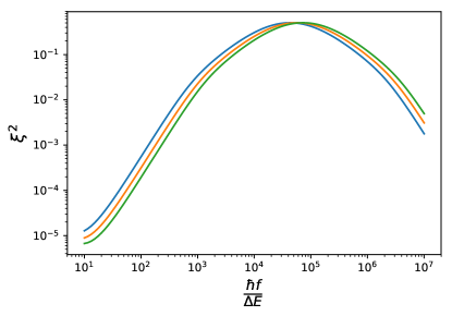
Figure 1: A plot of the phase sensitivity of quantum multibody states influenced by gravitational waves for different amplitude $h$. We set $P_{v}=1$, $t_{obs}=1$, and $N=50$. Blue, orange and green lines stand for $h=10^{-18}$, $h=10^{-21}$ and $h=10^{-24}$ respectively.

How about the change of $\xi^{2}$ with respect to amplitude $h$? We draw the lines in Fig. 2 to show the change of $\xi^{2}$ with respect to $h$ for different frequencies. It is clear from this figure that, for small frequency gravitational wave, $\xi^{2}$ increases with $h$ growing, but for large frequency, $\xi^{2}$ decreases with $h$ growing, which means that quantum entanglement may increase with increasing amplitude of gravitational waves. This phenomenon is counterintuitive but analogous to the celebrated anti-Unruh phenomena bmm16 ; lzy18 where entanglement could also be amplified with increasing acceleration. This is a novel phenomena which has not been found before, and show that entanglement is increased by the increasing gravitational magnitude, which is different from the view from the gravitational decoherence bgu17 .

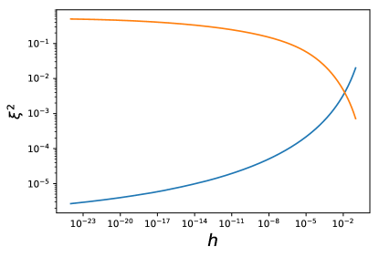
Figure 2: A plot of the spin-squeezing parameter of quantum multibody states influenced by gravitational waves as a function of the amplitude $h$ for different frequencies. Blue and orange lines stand for $f=1$ and $f=10^{4}$, respectively. $N=20$ and other parameters are the same as Fig. 1.

IV Experimental possibility

In order to check the size of the influence from the gravitational waves, we consider the experiment of the Ramsey interferometer nr85 ; ymk86 with the initial input state $\rho_{i}$, and the output state $\rho_{o}=U_{R}^{\dagger}\rho_{i}U_{R}$ where $U_{R}=exp(-i\theta J_{y})$ is the unitary operator for the evolution and $\theta$ is the phase shift. A main thought is to calculate the phase sensitivity for comparing the measurement results by taking the TF state and the state in Eq. (24) as the initial states. This gives whether the influence of gravitational waves on the TF state can be observed. Using the error propagation formula, $(\Delta\theta)^{2}=\frac{((\Delta J_{z}^{2})_{out})^{2}}{|d\langle J_{z}^{2}\rangle_{out}/d\theta|^{2}}$, the optimal phase sensitivity is given as mwn11

$$(\Delta\theta)_{opt}^{2}=\frac{\Delta J_{z}^{2}\Delta J_{x}^{2}}{2(\langle J_{x}^{2}\rangle-\langle J_{z}^{2}\rangle)^{2}}+\frac{V_{xz}}{4(\langle J_{x}^{2}\rangle-\langle J_{z}^{2}\rangle)^{2}},$$ (26)

where the optimal phase shift satisfies $tan^{2}\theta_{opt}=\Delta J_{z}^{2}/\Delta J_{x}^{2}$, $V_{xz}=\langle(J_{x}J_{z}+J_{z}J_{x})^{2}\rangle_{i}+\langle J_{z}^{2}J_{x}^{2}+J_{x}^{2}J_{z}^{2}\rangle_{i}-2\langle J_{z}^{2}\rangle_{i}\langle J_{x}^{2}\rangle_{i}$, and $(\Delta J_{x})^{2}=\langle J_{x}^{2}\rangle-\langle J_{x}\rangle^{2}$. When the initial state takes $\rho_{t}$ in Eq. (24), the results are presented in Fig. 3. From the Fig. 3, it is seen that the peak of the phase sensitivity curves will be shifted toward larger frequency when the amplitude of gravitational waves decreases, which has similar behaviors to that for spin-squeezing parameters in Fig. 1. Moreover, the increase of atomic number can improve the phase sensitivity as seen in Fig. 4 as expected.

When the initial state takes TF state without being influenced by gravitational waves, the phase sensitivity is obtained as

$$(\Delta\theta)_{TF}^{2}=1/(2j(j+1)),$$ (27)

which gives the phase sensitivity with $\sqrt{\frac{2}{N(N+2)}}$ approaching the the Heisenberg limit ps09 . For $N=50$ as taken in Fig. 4, the phase sensitivity is estimated as $(\Delta\theta)_{TF}^{2}\sim 7.7\times 10^{-4}$. There would be an increase in the value of phase sensitivity after the influence of gravitational waves. This means that it is possible to detect the influence in experiment if the initial state is exactly prepared as the TF state.

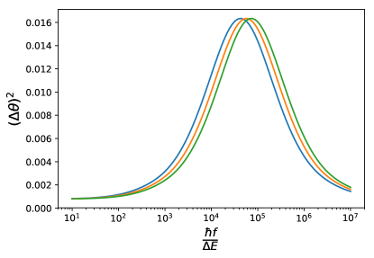
Figure 3: A plot of the phase sensitivity of quantum multibody states influenced by gravitational waves for different amplitude $h$. Blue, orange and green lines stand for $h=10^{-18}$, $h=10^{-21}$, and $h=10^{-24}$, respectively. Other parameters are the same as Fig. 1.

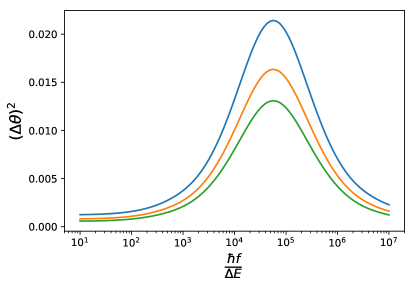
Figure 4: A plot of the phase sensitivity of quantum multibody states influenced by gravitational waves as a function of the frequency for different atom number. Blue, orange and green lines stand for $N=40$, $N=50$, and $N=60$, respectively. Other parameters are the same as Fig. 1.

But actually, a standard TF state is hard to be prepared in the present experimental conditions. In the experiment in lty17 , there are actually some factors leading to a deviation of standard TF state, e.g. the influence of nonaidabatic excitations and the atom loss which causes the quantum multibody state to be a mixture of Dicke state but not a standard TF state. For simplicity, we consider the mixture of Dicke state as $\rho_{i}=\sum_{j,m}p_{j,m}|j,m\rangle\langle j,m|$ where $p_{j,m}=p_{j}p_{m}$, and both $p_{j}$ and $p_{m}$ satisfy the Gaussian distribution, $p_{j}=\frac{1}{\sqrt{2\pi}\sigma_{j}}e^{-\frac{(j-\overline{j})^{2}}{2\sigma_{j}^{2}}}$, $p_{m}=\frac{1}{\sqrt{2\pi}\sigma_{m}}e^{-\frac{m^{2}}{2\sigma_{m}^{2}}}$ ($\sigma_{j},\sigma_{m}\ll\overline{j}$). When all atoms are influenced by the same gravitational waves, the Dicke state $|a,b\rangle$ becomes

$$\rho_{Dicke}=\sum_{m=-a}^{a}B_{m}^{2}|a,m\rangle\langle a,m|,$$ (28)

where $B_{m}^{2}=\sum_{k=0}^{\min{a-m,a+b}}C_{a-b}^{m-b+k}C_{a+b}^{k}P_{+}^{m-b+k}P_{-}^{k}$ for $m\geq b$ and $B_{m}^{2}=\sum_{k=0}^{\min{a+m,a-b}}C_{a-b}^{k}C_{a+b}^{b-m+k}P_{+}^{k}P_{-}^{b-m+k}$ for $m<b$.

We have calculated the change of entanglement related spin-squeezing parameter for a mixture of Dicke state influenced by gravitational waves. It is clear from Fig. 5 that for both of the two initial states, the spin-squeezing parameter first increases and then decreases with growing frequency, i.e., the amount of quantum entanglement for quantum-multibody states first decreases to a specific value and then increases slowly. Given that the spin-squeezing parameter for an initial mixed Dicke state is not zero at first, the change of spin squeezing for a mixed Dicke state seems less than a TF state, which means that it is more difficult to detect gravitational waves using a mixture of Dicke states, so it is important to prepare standard TF state as gravitational waves detectors.

When the real experimental values are used, the changes of spin squeezing induced by gravitational waves are so small that we actually cannot discern that with a TF state or mixed Dicke state of $11,000$ atoms, but if the atomic number increases, the influence of gravitational waves can be observed obviously by the change of the phase sensitivity. For example, the atomic number is given as $10^{28}$ as in the recent suggestion using BEC to detect gravitational waves ram19 , the phase sensitivity will increase $5$ orders of magnitude before and after the influence of gravitational waves for the initial TF state according to our calculation in Eq. (26). There is another method to improve the sensitivity by decreasing the spin-squeezing parameter or increasing entanglement of the initial multibody quantum states. This is shown in Fig. 6, which gives the sensitivity curves for detecting gravitational waves with different spin-squeezing parameters. It shows that the initial quantum state should be close enough to the TF state, which is still out of the present experimental range.

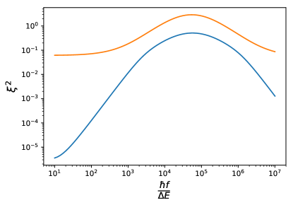
Figure 5: A plot of the spin squeezing parameter of quantum multi-body states influenced by gravitational waves as a function of the frequency. Blue and orange lines stand for TF state and mixed Dicke state respectively. We set atom number $N=20,\overline{j}=10,\overline{m}=0,\sigma_{j}=0.5,\sigma_{m}=0.5$, and other parameters are the same as Fig.1.

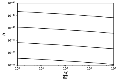
Figure 6: A plot of the spin squeezing parameter of TF states influenced by gravitational waves as a function of the frequency and amplitude. We set $t_{obs}=10^{6}\ s$, $N=11,000$, $P_{v}=100$ and $\Delta E=2\pi\hbar\ J$. The four black lines represent $\xi^{2}=10^{-47}$, $\xi^{2}=10^{-49}$, $\xi^{2}=10^{-51}$, $\xi^{2}=10^{-53}$ respectively from top to bottom.

V Conclusion

In this paper, we investigate the effect of gravitational waves on a single Unruh-Dewitt detector. We extended this work to quantum multibody states. We study the change of entanglement for the initial TF state by the influence of gravitational waves using the spin-squeezing parameter. It is found that there is a peak for every curve of the spin-squeezing parameters with different amplitudes of gravitational waves. In particular, we find that when the proper frequency of gravitational waves is chosen, the spin-squeezing parameter decreases with the increasing amplitude of gravitational waves. This means that entanglement increases when the field of gravitational waves becomes stronger and stronger, which is similar to the change of entanglement in the anti-Unruh effect caused by the acceleration. We also estimate the feasibility of experimental observation using the phase sensitivity, which is far from the present conditions. Such study is worthwhile and novel for understanding the behaviors of gravitational waves using their interaction with the quantum physical states.

VI Acknowledgments

This work is supported by National Natural Science Foundation of China (NSFC) with Grant No. 12375057, and the Fundamental Research Funds for the Central Universities, China University of Geosciences (Wuhan) with No. G1323523064.

References

- (1) A. Peres and D. R. Terno, Rev. Mod. Phys. 76, 93 (2008).
- (2) L. C. B. Crispino, A. Higuchi, and G. E. A. Matsas, Rev. Mod. Phys. 80, 787 (2008).
- (3) Y. Ma, H. Miao, B. H. Pang, M. Evans, C. Zhao, J. Harms, S. Roman, Y. Chen, Nat. Phys. 13, 776 (2017).
- (4) J. Südbeck, S. Steinlechner, M. Korobko, and R. Schnabel, Nat. Photonics 14, 240 (2020).
- (5) E. Knyazev, S. Danilishin, S. Hild, and F. Y. Khalili, Phys. Lett. A 382, 2219 (2018).
- (6) F. Gray, D. Kubiznak, T. May, S. Timmerman, and E. Tjoa, J. High Energy Phys. 11 (2021) 054.
- (7) J. Paczos, K. Dbski, P. T. Grochowski, A. R. H. Smith, and A. Dragan, arXiv:2204.10609.
- (8) Q. Xu, S. AliAhmad, and A. R. H. Smith, Phys. Rev. D 102, 065019 (2020).
- (9) T. Prokopec, arXiv:2206.10136.
- (10) R. V. Haasteren and T. Prokopec, arXiv:2204.12930.
- (11) Y. Li, B. Zhang, and L. You, New J. Phys. 24, 093034 (2022).
- (12) C. Sabín, D. E. Bruschi, M. Ahmadi, and I. Fuentes, New J. Phys. 16, 085003 (2014).
- (13) M. P. G. Robbins, N. Afshordi, and R. B. Mann, J. Cosmol. Astropart. Phys. 07, 032 (2019).
- (14) M. P. G. Robbins, N. Afshordi, A. O. Jamison, and R. B. Mann, Classical Quantum Gravity 39, 175009 (2022).
- (15) W. G. Unruh, Phys. Rev. D 14, 870 (1976).
- (16) B. S. DeWitt, S. Hawking and W. Israel, General Relativity: an Einstein Centenary Survey, (Cambridge University Press, Cambridge, England, 1979).
- (17) C. W. Misner, K. S. Thorne, and J. A. Wheeler, Gravitation, (W. H. Freeman and Company, USA, 1973).
- (18) N. D. Birrell and P. C. W. Davies, Quantum Fields in Curved Space (Cambridge University Press, Cambridge, England, 1984).
- (19) S. Takagi, Prog. Theor. Phys. Suppl. 88, 1 (1986).
- (20) R. H. Dicke, Phys. Rev. 93, 99 (1954).
- (21) J. Ma, X. Wang, C. P. Sun, and F. Nori, Phys. Rep. 509, 89 (2011).
- (22) A. Sørensen, L. Duan, J. Cirac, and P. Zoller, Nature (London) 409, 63 (2001).
- (23) G. Tóth, C. Knapp, O. Gühne, and H. J. Briegel, Phys. Rev. A 79, 042334 (2009).
- (24) O. Gühne and G. Tóth, Phys. Rep. 474, 1 (2009).
- (25) W. G. Brenna, R. B. Mann, and E. Martín-Martínez, Phys. Lett. B 757, 307 (2016).
- (26) T. Li, B. Zhang, and L. You, Phys. Rev. D 97, 045005 (2018).
- (27) A. Bassi, A. Großardt, and H. Ulbricht, Classical Quantum Gravity 34, 193002 (2017).
- (28) N. Ramsey, Molecular Beams (Oxford University Press, Oxford, England, 1985).
- (29) B. Yurke, S. L. McCall, and J. R. Klauder, Phys. Rev. A 33, 4033 (1986).
- (30) L. Pezzé and A. Smerzi, Phys. Rev. Lett. 102, 100401 (2009).
- (31) X.-Y. Luo, Y.-Q. Zou, L.-N. Wu, Q. Liu, M.-F. Han, M. K. Tey, and L. You, Science 355, 620 (2017).