An adaptive standardisation model for Day-Ahead electricity price forecasting

Abstract

The study of Day-Ahead prices in the electricity market is one of the most popular problems in time series forecasting. Previous research has focused on employing increasingly complex learning algorithms to capture the sophisticated dynamics of the market. However, there is a threshold where increased complexity fails to yield substantial improvements. In this work, we propose an alternative approach by introducing an adaptive standardisation to mitigate the effects of dataset shifts that commonly occur in the market. By doing so, learning algorithms can prioritize uncovering the true relationship between the target variable and the explanatory variables. We investigate four distinct markets, including two novel datasets, previously unexplored in the literature. These datasets provide a more realistic representation of the current market context, that conventional datasets do not show. The results demonstrate a significant improvement across all four markets, using learning algorithms that are less complex yet widely accepted in the literature. This significant advancement unveils opens up new lines of research in this field, highlighting the potential of adaptive transformations in enhancing the performance of forecasting models.

[label1]organization=Fortia Energía, addressline=Calle de Gregorio Benítez, city=Madrid, postcode=28043, country=Spain

[label2]organization=Universidad Politécnica de Madrid, city=Madrid, country=Spain

[label3]organization=Departamento de Matemática Aplicada a la Ingeniería Industrial, Escuela Técnica Superior de Ingenieros Industriales, Universidad Politécnica de Madrid, addressline=Calle de José Gutiérrez Abascal, city=Madrid, postcode=28006, country=Spain

[label4]organization=Instituto de Ciencias Matemáticas (CSIC-UAM-UC3M-UCM), addressline=Calle Nicolás Cabrera, city=Madrid, postcode=28049, country=Spain

[label5]organization=Laboratorio de Estadística, Escuela Técnica Superior de Ingenieros Industriales, Universidad Politécnica de Madrid, addressline=Calle de José Gutiérrez Abascal, city=Madrid, postcode=28006, country=Spain

A new model for Day-Ahead electricity price forecasting is proposed.

The focus of the model is to perform an adaptive standardisation of the series to be predicted, making all the time points of the series comparable to each other.

Two new current data sets (2019-2023) are made public due to the lack of studies in the literature related to the current electricity market context.

The proposed model improves the results of the state-of-the-art, with statistical evidence, in four different markets and in two periods characterised by completely different behaviour, highlighting the robustness to different scenarios.

1 Introduction

Electricity is one of the most important commodities in today’s society. However, the operation of the electricity system presents major particularities that must be addressed such as the balance between production and consumption, the independent hourly or quarter-hourly scheduling of different markets, the technical constraints of the generation program related to the security of the network, etc. In addition, significant changes in its behaviour occur: the increasing presence of renewable energies, the dynamics of external prices that affect generation costs and the impact of socio-economical factors are some examples. This situation means that the electricity market is in a condition of constant change and great uncertainty, especially regarding prices. We illustrate the Spanish Day-Ahead market to reflect this phenomenon, but this kind of behaviour is similar in every European country (Figure 1).

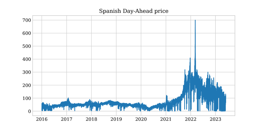
Figure 1: Spanish Day-Ahead market prices through the years

The observation of a discernible alteration in price dynamics towards the conclusion of 2021 becomes evident. As a result, we can observe three distinct phases: a period of stability, a subsequent phase characterized by increased volatility, and an intermediate transitory interval.

While the electricity market has been gaining attention over the years (Hong et al., 2020), and a rich literature related to the Day-Ahead market price forecasting has been developed (Lago et al., 2021), most studies focus on older stable periods that do not reflect the peculiarities of the current market.

This paper contributes to the existing literature as follows:

1. We propose a new model for Day-Ahead electricity price forecasting (EPF) that is characterized by ensuring comparability among all periods of the time series through an adaptive standardisation approach. This attribute makes the model flexible, allowing it to effectively respond to evolving situations and improve its performance accordingly.

2. We are providing access to two new datasets that span from 1st January 2019 to 31st May 2023. These datasets are made available not only for the purpose of replicating the results, but also to evaluate new models, enabling them to accurately reflect and represent the conditions of the current market.

3. An improvement is provided from a statistical perspective rather than from a machine learning perspective, which has been the main focus of research in recent years. This progress represents a significant development that has not been observed since Uniejewski et al. (2016).

The remainder of the paper is organized as follows: Section 2 performs a review of state-of-the-art trends and models in Day-Ahead EPF. Section 3 presents the novel model proposed and the rationale behind it. Finally, in Section 4 the models are tested and the results are discussed, ending with the conclusions in Section 5.

2 Previous work

2.1 Electricity price forecasting (EPF)

EPF is an open field in which a wide variety of tasks are included, mainly depending on the market being dealt with: Day-Ahead market, Intra-Day markets or Balancing markets. Among these, the Day-Ahead market has garnered the most significant attention. While the regulatory framework of this market varies across countries, its structure, as depicted in Figure 2, follows a standard pattern in Europe: on day D, prior to a designated hour H, all market participants are required to submit their bids for purchasing or selling energy for each hour of the subsequent day, D+1. The price of each hourly period is established independently through an auction-based format.

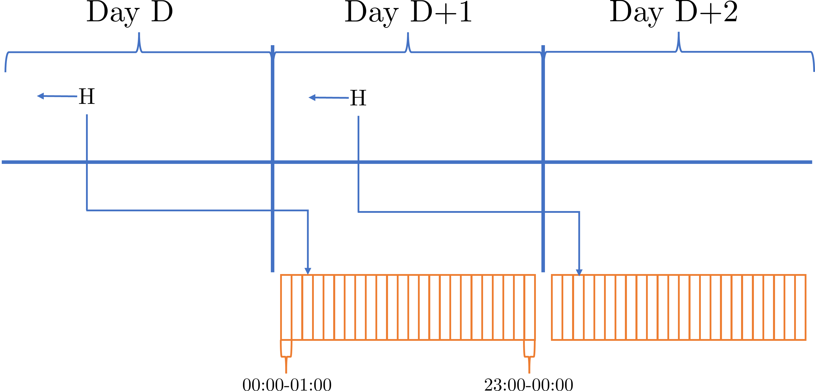
Figure 2: Structure of the Day-Ahead auction market

As explained in Ziel and Weron (2018), mainly two approaches can be considered in EPF and, indeed, in other forecasting problems of the electricity market:

1. Consider a high-frequency univariate time series, typically observed at an hourly interval, where a single global model is utilized for analysis and prediction.

2. Consider a multivariate time series, where the subsequent 24 hours must be predicted using a single multivariate model. This approach can be transformed in an univariate perspective by treating each hour independently and, therefore, using separate models for each hour.

The first option is the standard approach when working with machine learning models, as they typically require vast amounts of data. In contrast, the second option with 24 separate models, is commonly found in statistical models. However, according to Ziel and Weron (2018), neither approach dominates the other. It is the combination of both methods that yields superior results in terms of predictive performance.

In a distinct research direction, it has been studied the application of Functional Data Analysis (FDA) within the electricity market, as can be seen in Chen et al. (2021). FDA treats individual time series as discrete observations derived from a continuous function. Building upon this concept, two relevant studies focusing on price prediction are those by Chen and Li (2017) and Jan et al. (2022), both of which showcase promising outcomes and advancements in this domain.

Nevertheless, establishing state-of-the-art models in the field of EPF, particularly within the Day-Ahead market, presents a complex challenge due to a multitude of factors highlighted by Lago et al. (2021):

• It is typical for different studies to come to contradictory conclusions, especially when comparing classical statistical methods with machine learning techniques.

• Similarly, comparisons are often drawn with basic models that fall considerably short of achieving the performance levels exhibited by the best known models. Furthermore, studies often analyze datasets that have not been previously explored or documented in the existing literature.

• The test period is often relatively short, which introduces the possibility of overlooking special situations and failing to adequately assess the annual seasonality inherent in price dynamics. As a consequence, the obtained results may be influenced by the specific choice of the test window, potentially limiting their generalizability.

• Sometimes the results cannot be replicated, not allowing the results to be tested by other community members.

As we strongly agree with these statements, we align ourselves with the definition of state-of-the-art models as presented in the review by Lago et al. (2021).

The Lasso Estimated AutoRegressive (LEAR), proposed in Uniejewski et al. (2016), is considered as the best statistically based model. It is is an autoregressive model with exogenous variables (ARX) to which an L1 regularisation is applied.

The DNN proposed in Lago et al. (2018) is considered one of the best machine learning based models. It has a simple structure consisting of a fully connected neural network with two hidden layers and an output layer comprising 24 neurons, each corresponding to a specific hour. So, instead of having one model for each hour as in the previous case, there is just one model for the whole serie.

From a machine learning perspective, a new model has achieved better results: NBEATSx (Olivares et al., 2023), an extension of the NBEATS model (Oreshkin et al., 2019) that allows for the inclusion of exogenous variables. One advantage of NBEATSx is the ability to perform an analysis to understand how each potential source of information affects the predictions, which is not commonly found in models of this nature. When applied to typical datasets in the literature, the results obtained by this model are superior to those presented by the previously mentioned neural network. However, it is worth mentioning that the improvement achieved by NBEATSx may not always reach statistical significance in certain markets according to the Giacomini-White test (Giacomini and White, 2006) carried out by the authors. Another aspect to consider is the increase in computational complexity associated with this model.

The X-Model presented in Ziel and Steinert (2016) is also noteworthy, as it follows a completely different approach to the usual one. Instead of the classical time series modelling, it tries to model the supply and demand curves that determine the price for each hourly period. The results are quite positive, even capturing non-linear behaviour.

In the EPF context, it has been acknowledged that the behavior of the target series exhibits temporal variations. To address this issue, Nasiadka et al. (2022) propose the integration of change point methods, aiming to identify historical windows in the past that align with the current market conditions. These selected windows are then incorporated into the training set. However, it is important to recognize that these change point methods may not always accurately identify the relevant windows due to the complexity of the underlying market dynamics. The effectiveness of such methods relies on the assumption that the identified change points truly reflect the shifts in the market behavior. In practice, there can be instances where the change point detection may fail to capture the subtle nuances or abrupt changes in the series, leading to potential inaccuracies in the selection of training data. Moreover, a significant portion of the available information in the historical data remains unused. Thus, while change point methods offer a valuable approach, their limitations should be considered.

Although probabilistic forecasting is beyond the scope of this study, it is worth noting that a significant portion of the EPF field is devoted to this area. Therefore, it is necessary to mention some of the main works within this particular trend. A satisfactory idea was introduced in Nowotarski and Weron (2015): applying quantile regression (Koenker and Bassett Jr, 1978) using the predictions obtained by point estimators as explanatory variables (QRA). Given the good results of the LEAR model in point estimation, Uniejewski and Weron (2021) propose the use of quantile regression following the same philosophy, but applying L1 regularisation on the loss function, so that an automatic selection of variables is performed, improving the results. Complex recurrent or convolutional neural network structures in a probabilistic context are compared in Mashlakov et al. (2021) but focusing on the electricity market in general, not only on price. More classical techniques such as bootstrap over residuals (Efron, 1992) to obtain probabilistic results have also been used for price forecasting in the electricity market in Narajewski and Ziel (2021). A more in-depth study on the price appears in Marcjasz et al. (2023) through the use of distributional neural networks, used for the first time in this field. The results are better than those obtained by applying QRA to the LEAR model or to the neural network of Lago et al. (2018), although not entirely satisfactory as observed by the number of hours that pass the Kupiec test (Kupiec et al., 1995) at 50% and 90%. It is also worth mentioning that the use of the novel framework of conformal prediction (Vovk et al., 2005) has also been applied in EPF (Kath and Ziel, 2021), where it is concluded that valid prediction intervals can be obtained on the predictions made, improving on several metrics of QRA.

2.2 Adaptive transformation schemes

When referring to adaptive transformation methods, we specifically mean time series transformations that utilize a window of past observations rather than the entire historical data to achieve stationarity. It is important to note that we do not consider the use of rolling windows alone as a form of adaptive transformation because the models that employ rolling windows typically utilize data solely from within the window to process information and make predictions.

The first adaptive transformation technique was introduced in Ogasawara et al. (2010). In this case, a modified version of the conventional min-max normalization method is proposed to address specific challenges associated with the traditional approach, particularly those related to volatility. The technique is thoroughly analyzed across various non-stationary series, consistently showing better results.

In Passalis et al. (2019), a deep learning approach is employed. The proposed method, known as Dynamic Adaptive Input Normalization (DAIN), includes the data transformation as trainable parameters within the neural network architecture. This allows the optimal transformation to be learned and automatically adjusted during the training process, similar to other network parameters. In this way, each time the network is trained, it is calibrated to the current context of the system that is being predicted. Empirically, the results demonstrate an improvement when compared to conventional approaches.

Lastly, Gamakumara et al. (2023) propose an estimation technique for the conditional mean and conditional variance using Generalized Additive Models (GAM), (Hastie and Tibshirani, 1990). By employing GAM models, the estimation process allows the conditional standardisation of the data by effectively removing sources of variation external to the time series itself. Although this is not an adaptive transformation as such, this approach proves to be more suitable for non-stationary time series compared to classical methods, enabling improved modeling and analysis of the underlying dynamics.

3 Proposed methodology

A widely adopted methodology, regardless of whether statistical or machine learning-based methods are employed, is to transform non-stationary price series into a more stationary form before implementing the learning algorithm. This involves applying one of several available transformations that aim to achieve a constant mean and stabilize the variance (Uniejewski et al., 2017). Regardless of the transformation used, they are computed in the training set for subsequent application in the validation and test sets. However, it is important to acknowledge that this methodology assumes the absence of any change in the joint distribution of the data, implying no occurrence of dataset shift (Quiñonero-Candela et al., 2008). Nonetheless, a quick examination of Figure 1 shows the presence of potential shifts within the data.

Looking at the behaviour of prices, it is reasonable to consider that consecutive intervals of varying length in the time series exhibit stationarity, or at least a constant mean and variance. This means that the time series is piecewise stationary in mean and variance. In view of this fact, let $p_{d}^{h}$ be the price series corresponding to the hour $h$ in the day $d$, the following model is proposed

$$\begin{cases}p_{d}^{h}&=\mu(X_{d})+\sigma(X_{d})u_{d}^{h}\equiv\mu_{d}+\sigma_{d}u_{d}^{h}\\ u_{d+1}^{h}&=f(X_{d},u_{d}^{h},u_{d-1}^{h},\dots)+\varepsilon_{d+1}^{h}\end{cases}$$

We propose the following parameter estimation methodology:

$$\begin{cases}\hat{\mu_{d}}&=\dfrac{1}{24v}\displaystyle\sum_{k=d-v-1}^{d-1}\sum_{h=1}^{24}p_{k}^{h},\;\text{for each }d\\ \hat{\sigma_{d}}&=\sqrt{\dfrac{1}{24v}\displaystyle\sum_{k=d-v-1}^{d-1}\sum_{h=1}^{24}\left(p_{k}^{h}-\hat{\mu_{d}}\right)^{2}},\;\text{for each }d\\ \end{cases}$$ (1)

where $v$ is the lenght of a rolling window in days, $f$ is a learning algorithm and $X_{d}$ is the set of explanatory features available before the end of the biding period for day $d$.

Figure 3 presents a comparison between the current price series in the Spanish Day-Ahead market and the series obtained using a median-arcsinh standardisation scheme, which has been applied in the EPF literature (Uniejewski and Weron, 2018), and another series representing the $u_{d}^{h}$ process resulting from our proposed methodology.

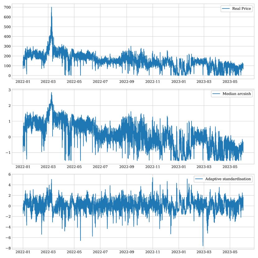
Figure 3: Comparison of the current price in the Spanish Day-Ahead market during hour 20 (top), its median-arsinh transformation (middle) and the resulting process derived of applying our methodology with $v=7$ days, 168 hours (bottom)

It is evident from the figure that our methodology yields a significantly more stationary series, which aligns with the main objective of applying such transformations. The fundamental idea of the transformation is to encapsulate the effects of potential shifts in the $\mu_{d}$ and $\sigma_{d}$ parameters, ensuring that the resulting process $u_{d}^{h}$ is minimally affected by such situations. Additionally, implementing the adaptive standardisation through a reasonably sized rolling window enables a rapid response to these shifts.

As this adaptive standardisation mitigates shifts in the behaviour of the price series, the unmodified explanatory features are sub-optimal candidates for the prediction of transformed prices. They also need to be transformed. Furthermore, this step is crucial to avoid spurious regressions caused by non-stationary explanatory variables (Harris and Sollis, 2003). We choose to apply the rolling standardisation of length $v$, with the parameters $\mu_{d}$ and $\sigma_{d}$ obtained in (1) to each one of the variables for non-dummy features and leave dummy features unchanged.

4 Experiments

To evaluate the results, a thorough analysis of the proposed methodology is conducted utilizing the established Python library epftoolbox (Lago et al., 2021). By comparing the use of a conventional transformation scheme in the EPF literature (median-arcsinh transformation) with the one we propose, we can show the significance of our approach and its impact on the final model. The models are retrained each day, as one should do in a real industrial EPF situation. For the adaptive standardisation, we have selected $v=7$ days ($168$ hours). This parameter has been selected empirically, after seeing that the window is not too large and the transformed series still retains the desired characteristics. Also, it seems reasonable to choose a one-week window from an expert perspective in the electricity market. Logically, $v$ can be chosen by the user based on the need of the problem to be solved.

4.1 Learning algorithms

We consider the LEAR model and the neural network both presented in Section 2 and available in the epftoolbox package, as potential learning algorithms $f$ (Equation 1)

4.1.1 LEAR

The model specification is

$$\begin{aligned} u_{d}^{h}=&\sum_{i=1}^{24}\theta_{h,i}\cdot u_{d-1}^{i}+\sum_{i=1}^{24}\theta_{h,24+i}\cdot u_{d-2}^{i}+\sum_{i=1}^{24}\theta_{h,48+i}\cdot u_{d-3}^{i}+\sum_{i=1}^{24}\theta_{h,72+i}\cdot u_{d-7}^{i}\\ &+\sum_{i=1}^{24}\theta_{h,96+i}\cdot x_{d,1}^{i}+\sum_{i=1}^{24}\theta_{h,120+i}\cdot x_{d,2}^{i}+\sum_{i=1}^{24}\theta_{h,144+i}\cdot x_{d-1,1}^{i}\\ &+\sum_{i=1}^{24}\theta_{h,168+i}\cdot x_{d-1,2}^{i}+\sum_{i=1}^{24}\theta_{h,192+i}\cdot x_{d-7,1}^{i}+\sum_{i=1}^{24}\theta_{h,216+i}\cdot x_{d-7,2}^{i}\\ &+\sum_{i=1}^{7}\theta_{h,240+i}\cdot\mathbf{z}_{d}+\varepsilon_{d}^{h}\end{aligned},$$

where $u_{d}^{h}$ is the standardised price ($p_{d}^{h}$) of day $d$ in hour $h$, $x_{d,1}^{h}$ and $x_{d,2}^{h}$ are two variables of interest associated with the market on day $d$ in hour $h$, usually related to load, wind forecasting or solar forecasting, and $\mathbf{z}_{d}$ is a binary vector representing the day of the week that is day $d$. The values of $x_{d,1}^{h},x_{d,2}^{h}$ may require a standardisation similar to that of the price. The $\varepsilon_{d}^{h}$ simply represents noise. Note that this is a model for each hour.

The coefficients of the model $\hat{\theta}_{h}=(\hat{\theta}_{h,1},\dots,\hat{\theta}_{h,247})$ are calculated as

$$\hat{\theta}_{h}=\operatorname*{\arg\!\min}_{\theta_{h}}\sum_{d=1}^{N_{d}}(u_{d}^{h}-\hat{u}_{d}^{h})^{2}+\lambda\sum_{i=1}^{247}|\theta_{h,i}|$$

with $\hat{u}_{d}^{h}$ the forecast of day $d$ at hour $h$, $N_{d}$ the number of days in the training set and $\lambda$ a regularization hyperparameter of the model that can be fitted across a multitude of schemes.

4.1.2 DNN

We also consider the DNN proposed in Lago et al. (2018) as a representative of the machine learning based models. The model parameters are estimated through the utilization of the Adam optimization algorithm (Kingma and Ba, 2014). We employ the same set of potential input features as employed in the LEAR model. The selection of specific input features is determined as another hyperparameter of the network. To optimize these hyperparameters, we employ a tree-structured Parzen estimator (Bergstra et al., 2011). Notably, hyperparameters unrelated to the explanatory features encompass the following: the number of neurons per layer, the choice of activation function, the dropout rate, the learning rate, the inter-layer normalization scheme, preprocessing procedures prior to the input layer, weight initialization strategies, and the coefficient associated with the applied L1 regularization.

4.2 Datasets

To ensure the generalizability of the results, it is crucial to consider multiple markets. In this paper, we analyze four datasets, two of which are novel contributions to the literature. These datasets are in the public domain and we make them available to the research community, as they offer valuable opportunities for studying and addressing market conditions that are more representative of the current state. The four markets to consider are (Figure 4):

• The OMIE-SP market, representing the Spanish electricity market. This market is not available in the Python package. Price data spans from January 1st, 2019 to May 31st, 2023. Two explanatory variables, namely the day-ahead load forecast and the forecast of renewable energy generation (solar photovoltaic, solar thermal and wind). The data has been obtained through the ESIOS platform.

• The EPEX-DE market, representing the German electricity market, is another dataset considered in this study. Data from January 1st, 2019 to May 31st, 2023 has been obtained from the ENTSO-E transparency platform. Similar to the previous market, the same exogenous variables have been considered. However, in this case, the renewable generation forecast does not include the solar thermal generation forecast.

• The EPEX-FR market, which is the Day-Ahead electricity market in France. The dataset also encompasses the period from January 9th, 2011 to December 31st, 2016. It incorporates two exogenous variables: the day-ahead load and generation forecasts from France. The dataset is accessible from the epftoolbox package.

• The EPEX-BE market, which is the Day-Ahead electricity market in Belgium. The dataset encompasses the period from January 9th, 2011 to December 31st, 2016. It incorporates the same two exogenous variables from France, which, although surprising, are two of the best regressors for this market (Lago et al., 2018). The dataset is accessible from the epftoolbox package.

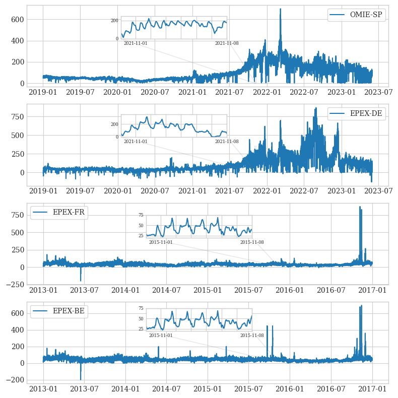
Figure 4: Markets considered. Observe the differences between the variability of one of the current markets and one of the previous markets.

Due to their smaller size and specific focus on high volatility and market uncertainty, the first two cases are evaluated using a testing period of one year and five months. This corresponds to the entire year of 2022 and all available data for 2023. In the last two cases, the evaluation of the models includes a testing period of two years, specifically the entirety of 2015 and 2016. It is crucial that the test periods span at least one year. This duration allows for the inclusion of all the seasonal variations present throughout the year, as well as the consideration of specific events or occasions that may impact market behavior, such as holidays.

In all of the considered datasets, the LEAR model is evaluated using rolling windows of 2 years, 1 year, and 6 months. For the DNN model, a rolling window of 3 years is used for the first two cases due to size limitations, which are new instances, while for the last two cases a window of 4 years is employed. Additionally, when applying adaptive standardisation, the entire available data (excluding the day to be predicted) is used for training and validation. The use of rolling windows is justified as it allows the models to adapt to the various changes present in the time series. However, in our proposed model, the series appears to be comparable at all instances, suggesting that the use of rolling windows may not be necessary if all changes are effectively captured in the parameters $\mu_{d}$ and $\sigma_{d}$.

4.3 Outliers treatment

Another fact that must be taken into account is that the proposed method could be highly sensitive to the presence of large outliers because they could significantly impact the estimation of $\mu_{d}$ and $\sigma_{d}$, which are crucial components of the adaptive transformation process. This can be seen in Figure 5, where the application of the methodology as described in Section 3 is negatively affected by the presence of such observations. However, it is worth noting that once the outliers no longer influence the window used for applying the adaptive transformation, the model performs adequately.

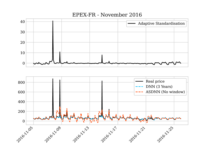
Figure 5: The first series shows the result of applying the adaptive standardisation in November 2016 in France. The large increase in the standard deviation in the areas after outliers makes the transformed value very close to 0. In the second series we can see the effect that the presence of outliers has on the Adaptive Standardisation DNN model (ASDNN) compared with the predictions of the DNN model.

In response to this situation two analysis will be conducted: first, the different models will be studied ignoring the outliers and, after that, every experiment will be repeated with a preliminary step focused on mitigating the impact of outliers. This step, described in A, aims to address these outliers and reduce their influence on the modeling process. The outlier mitigation process can be seen as a form of intervention in the time series, similar to addressing specific anomalous days or events, so the model proposed in Equation (1) still aligns with this new methodology. The models that have undergone an outlier mitigation process are indicated by an “O” prefix before their names.

It is worth noting that such outlier mitigation methodologies are not very popular in the EPF literature, so the two analysis have a dual function: to confirm that these methodologies, on top of existing models, do not produce better results and to observe the behaviour of the new model proposed in this paper in the presence or absence of such observations.

4.4 Evaluation metrics

Four accepted metrics in the forecasting literature are used to measure the quality of outcomes:

• MAE $=\dfrac{1}{24N_{d}}\displaystyle\sum_{d=1}^{N_{d}}\sum_{h=1}^{24}|p_{d}^{h}-\hat{p}_{d}^{h}|$

• RMSE $=\sqrt{\dfrac{1}{24N_{d}}\displaystyle\sum_{d=1}^{N_{d}}\sum_{h=1}^{24}\left(p_{d}^{h}-\hat{p}_{d}^{h}\right)^{2}}$

• sMAPE $=\dfrac{1}{24N_{d}}\displaystyle\sum_{d=1}^{N_{d}}\sum_{h=1}^{24}2\dfrac{|p_{d}^{h}-\hat{p}_{d}^{h}|}{|p_{d}^{h}|+|\hat{p}_{d}^{h}|}$

• rMAE $=\dfrac{\dfrac{1}{24N_{d}}\displaystyle\sum_{d=1}^{N_{d}}\sum_{h=1}^{24}|p_{d}^{h}-\hat{p}_{d}^{h}|}{\dfrac{1}{24N_{d}}\displaystyle\sum_{d=1}^{N_{d}}\sum_{h=1}^{24}|p_{d}^{h}-p_{d}^{h,\,\text{naive}}|}$

where $N_{d}$ is the number of days in the test set and $p_{d}^{h}$, $\hat{p}_{d}^{h}$, $p_{d}^{h,\,\text{naive}}$ are the current price, the prediction and the prediction by a naive model of the hour $h$ on day $d$, respectively. In the EPF field, is common to consider

$$p_{d}^{h,\,\text{naive}}=\begin{cases}p_{d-1}^{h}&\text{if }d\text{ is Tue, Wed, Thu or Fri}\\ p_{d-7}^{h}&\text{if }d\text{ is Sat, Sun, or Mon}\end{cases}$$

4.4.1 Results

Tables 1, 2, 3 and 4 show the evaluation metrics for the mentioned datasets without the outlier mitigation process and Tables 5, 6, 7 and 8 with it. We will adopt the notation “AS” before each model name to indicate that it incorporates the adaptive standardisation approach.

	LEAR (2 Years)	LEAR (1 Year)	LEAR (6 Months)	DNN (3 Years)	ASLEAR (No window)	ASLEAR (2 Years)	ASLEAR (1 Year)	ASLEAR (6 Months)	ASDNN (No window)
MAE	19.46	19.4	19.75	19.0	18.29	18.51	18.71	18.97	17.93
RMSE	27.57	27.96	28.43	27.04	25.93	26.19	26.84	27.05	25.49
sMAPE	0.22	0.22	0.22	0.21	0.21	0.21	0.21	0.21	0.21
rMAE	0.65	0.65	0.66	0.64	0.61	0.62	0.63	0.63	0.6

Table 1: Evaluation metrics for the OMIE-SP dataset

	LEAR (2 Years)	LEAR (1 Year)	LEAR (6 Months)	DNN (4 Years)	ASLEAR (No window)	ASLEAR (2 Years)	ASLEAR (1 Year)	ASLEAR (6 Months)	ASDNN (No window)
MAE	28.54	30.67	28.86	27.29	26.11	26.01	26.47	27.37	25.4
RMSE	40.6	42.52	41.89	39.13	38.86	38.65	39.14	40.12	37.15
sMAPE	0.23	0.25	0.24	0.22	0.22	0.22	0.22	0.23	0.22
rMAE	0.51	0.55	0.52	0.49	0.47	0.47	0.47	0.49	0.46

Table 2: Evaluation metrics for the EPEX-DE dataset

	LEAR (2 Years)	LEAR (1 Year)	LEAR (6 Months)	DNN (4 Years)	ASLEAR (No window)	ASLEAR (2 Years)	ASLEAR (1 Year)	ASLEAR (6 Months)	ASDNN (No window)
MAE	4.22	4.25	4.53	4.12	4.65	4.68	4.88	5.83	4.29
RMSE	11.69	11.28	11.78	11.97	13.39	16.27	19.86	56.38	11.6
sMAPE	0.13	0.13	0.13	0.12	0.12	0.13	0.13	0.13	0.12
rMAE	0.71	0.71	0.76	0.69	0.78	0.78	0.82	0.98	0.72

Table 3: Evaluation metrics for the EPEX-FR dataset

	LEAR (2 Years)	LEAR (1 Year)	LEAR (6 Months)	DNN (4 Years)	ASLEAR (No window)	ASLEAR (2 Years)	ASLEAR (1 Year)	ASLEAR (6 Months)	ASDNN (No window)
MAE	6.4	6.52	6.83	6.45	7.7	7.76	8.12	9.63	7.21
RMSE	16.47	16.07	16.18	16.84	19.19	20.28	22.38	42.19	18.08
sMAPE	0.15	0.16	0.16	0.15	0.17	0.17	0.18	0.19	0.16
rMAE	0.78	0.79	0.83	0.78	0.94	0.94	0.99	1.17	0.88

Table 4: Evaluation metrics for the EPEX-BE dataset

	OLEAR (2 Years)	OLEAR (1 Year)	OLEAR (6 Months)	ODNN (3 Years)	OASLEAR (No window)	OASLEAR (2 Years)	OASLEAR (1 Year)	OASLEAR (6 Months)	OASDNN (No window)
MAE	22.13	22.23	22.81	24.1	20.41	21.24	22.2	22.81	22.33
RMSE	32.82	32.46	33.54	35.11	30.33	31.42	32.9	33.59	32.28
sMAPE	0.24	0.23	0.24	0.24	0.23	0.23	0.23	0.24	0.25
rMAE	0.74	0.74	0.76	0.81	0.68	0.71	0.74	0.76	0.75

Table 5: Evaluation metrics for the OMIE-SP dataset with the outlier mitigation process

	OLEAR (2 Years)	OLEAR (1 Year)	OLEAR (6 Months)	ODNN (3 Years)	OASLEAR (No window)	OASLEAR (2 Years)	OASLEAR (1 Year)	OASLEAR (6 Months)	OASDNN (No window)
MAE	34.06	35.44	36.85	33.49	32.46	34.05	36.05	36.96	32.24
RMSE	51.43	52.28	55.26	52.78	52.33	54.14	56.59	57.43	51.01
sMAPE	0.26	0.27	0.27	0.25	0.24	0.25	0.26	0.27	0.24
rMAE	0.61	0.63	0.66	0.6	0.58	0.61	0.65	0.66	0.58

Table 6: Evaluation metrics for the EPEX-DE dataset with the outlier mitigation process

	OLEAR (2 Years)	OLEAR (1 Year)	OLEAR (6 Months)	ODNN (4 Years)	OASLEAR (No window)	OASLEAR (2 Years)	OASLEAR (1 Year)	OASLEAR (6 Months)	OASDNN (No window)
MAE	4.38	4.4	4.72	4.36	4.04	4.01	4.07	4.25	4.09
RMSE	12.24	12.19	12.59	12.44	11.82	11.83	11.9	12.04	11.92
sMAPE	0.13	0.13	0.14	0.12	0.12	0.11	0.12	0.12	0.12
rMAE	0.73	0.74	0.79	0.73	0.68	0.67	0.68	0.71	0.68

Table 7: Evaluation metrics for the EPEX-FR dataset with the outlier mitigation process

	OLEAR (2 Years)	OLEAR (1 Year)	OLEAR (6 Months)	ODNN (4 Years)	OASLEAR (No window)	OASLEAR (2 Years)	OASLEAR (1 Year)	OASLEAR (6 Months)	OASDNN (No window)
MAE	6.51	6.6	6.82	6.21	6.16	6.27	6.33	6.49	6.19
RMSE	17.1	16.95	17.13	16.78	16.53	16.63	16.61	16.79	16.68
sMAPE	0.15	0.16	0.16	0.14	0.14	0.15	0.15	0.15	0.14
rMAE	0.79	0.8	0.83	0.76	0.75	0.76	0.77	0.79	0.75

Table 8: Evaluation metrics for the EPEX-BE dataset with the outlier mitigation process

The analysis of the obtained metrics reveals a clear improvement in results when applying adaptive standardisation to the OMIE-SP and EPEX-DE markets (Tables 1 and 2). However, this improvement is not observed for the EPEX-FR and EPEX-BE markets in a first instance as shown by Tables 3 and 4. To further investigate this situation, we propose the use of a dynamic evaluation approach, specifically examining the month-to-month MAE (for example) on the test set. We suggest incorporating such methodologies into model evaluation to assess whether improvements are consistently observed throughout the entire time period or if they occur selectively in specific cases over time. Figures 6, 7, 8 and 9 show this for each market without the outlier treatment. Only one reference model from each family, the one that performs the best overall in each case, has been considered to make the graph more readable.

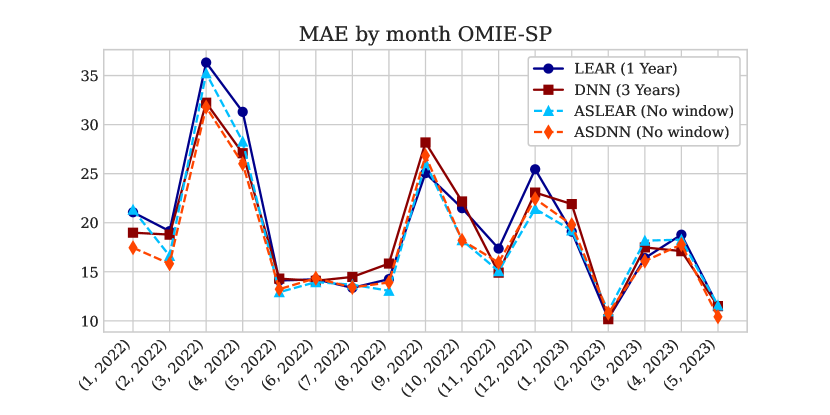
Figure 6: MAE by month in the OMIE-SP market

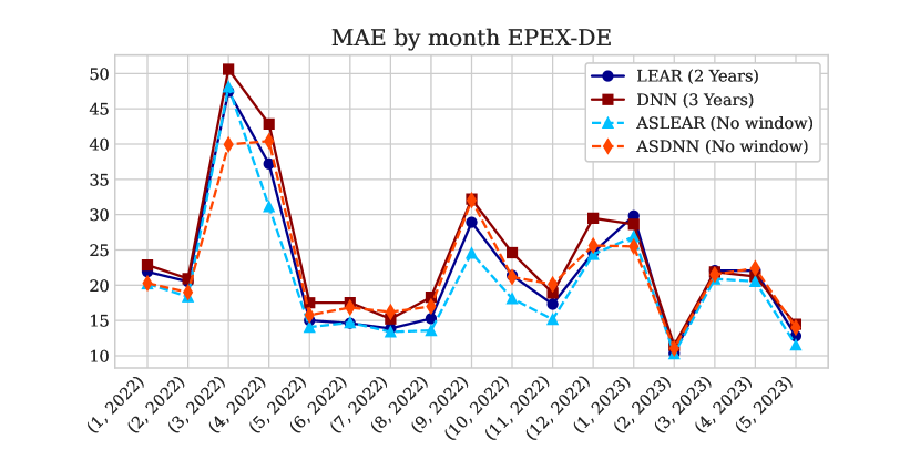
Figure 7: MAE by month in the EPEX-DE market

For the OMIE-SP (Figure 6) and EPEX-DE markets (Figure 7), it can be observed that the improvement is consistent throughout the entire test period. In most cases, either the ASLEAR model or the ASDNN model performs the best in terms of MAE for each month.

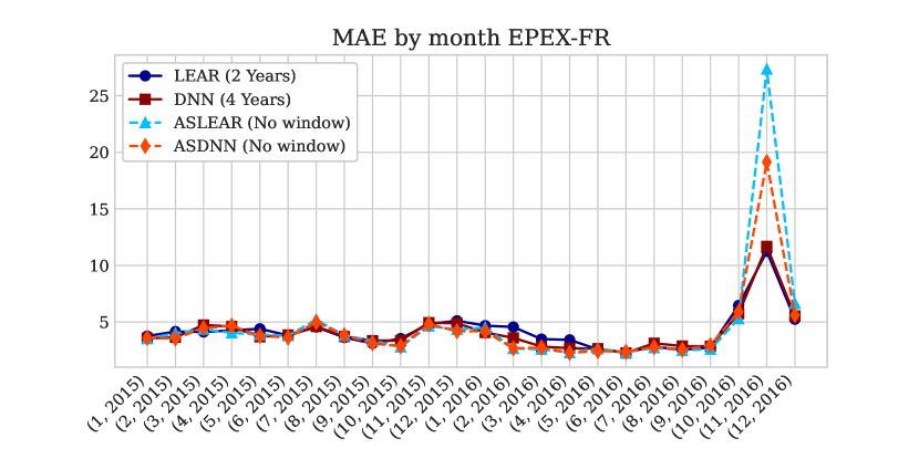
Figure 8: MAE by month in the EPEX-FR market

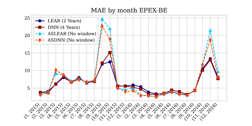
Figure 9: MAE by month in the EPEX-BE market

For the EPEX-FR (Figure 8) and EPEX-BE (Figure 9) markets, a similar pattern is observed, where the adaptive standardisation models perform the best in most months or at least on par. However, in both cases, there are specific months where the error increases significantly.

If we analyze the predictions of the different models of those months in detail, we encounter a situation very similar to the one observed in Figure 5. That means that the model is not performing well in the presence of outliers. For the French and Belgian markets, it can be observed how the error decreases as the effect of outliers is attenuated (Tables 7 and 8). However, this characteristic only occurs with the adaptive standardisation models. For the other two markets, no model benefits from this previous treatment (Tables 5 and 6).

The two hypotheses that we wanted to analyse by studying the treatment of outliers have been confirmed. First, if there are no clear outliers, their treatment over the non-adaptive models is not necessary, as these observations probably provide a large amount of information to the models, helping to obtain better predictions in the future, as other works in the literature show. Second, such treatment is vital for the good performance of the adaptive standardisation in the presence of large price spikes.

If we apply the preprocessing phase in the French and Belgian markets, performance improvements can be observed when using adaptive standardisation. This occurs despite the high stability of these two series, where a traditional non-adaptive treatment when transforming the variables could be completely valid. Figure 10 shows the differences in predictions between the best model without and with adaptive standardisation for the EPEX-BE market in a certain period. It can be seen how the proposed model is capable of capturing a behaviour that is not present in the rest of the models, even in this type of series that are already fairly stationary.

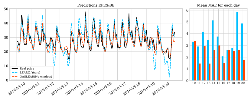
Figure 10: Predictions in the EPEX-BE market.

Figures 11 and 12 show the month-to-month performance of applying the outlier treatment in our proposal versus not applying it in the other models (which is how they perform best) for these two markets. It can now be seen how the MAE peaks in those problematic months are mitigated, leading to a better overall performance. We stress the importance of using a dynamic metric to detect such errors, as the overall performance of the proposed model was better or similar to the other models.

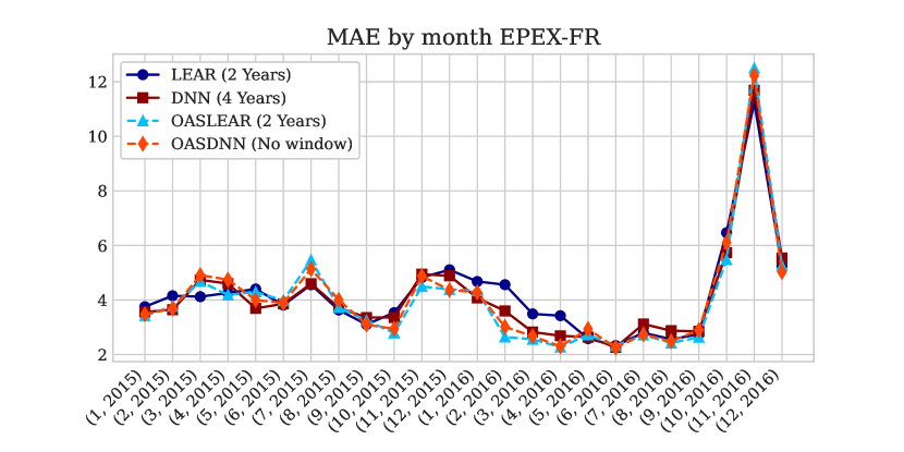
Figure 11: MAE by month in the EPEX-FR market with the best models of each category

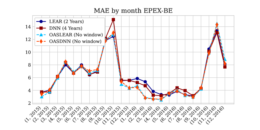
Figure 12: MAE by month in the EPEX-BE market with the best models of each category

4.5 Statistical testing

It is important to analyze whether the difference between predictions from different models is statistically significant. In the context of EPF, the Diebold-Mariano test (Diebold and Mariano, 2002) is used for this purpose.

The Diebold-Mariano test involves evaluating the hypothesis that $\mathbb{E}\left(\Delta_{d,h}^{A,B}\right)$ is zero, where $\Delta_{d,h}^{A,B}=L(\varepsilon_{d,h}^{A})-L(\varepsilon_{d,h}^{B})$ and $\varepsilon_{d,h}^{Z}=p_{d}^{h}-\hat{p}_{d}^{h}$ represents the prediction error of model $Z$ for day $d$ at hour $h$, and $L$ is the loss function being considered. In this case, we will consider the absolute loss.

The statistic $\text{DM}=\sqrt{N}\dfrac{\hat{\mu}}{\hat{\sigma}}$ is computed, where $\hat{\mu}$ and $\hat{\sigma}$ represent the mean and standard deviation of $\Delta_{d,h}^{A,B}$, respectively, and $N$ is the number of observations in the test period. The test statistic asymptotically follows a standard normal distribution. In this way, the computation of the p-value associated with the test

$$\begin{cases}H_{0}:&\mathbb{E}\left(\Delta_{d,h}^{A,B}\right)\leq 0\\ H_{1}:&\mathbb{E}\left(\Delta_{d,h}^{A,B}\right)>0\end{cases}$$

can be obtained.

If the null hypothesis is rejected, it indicates that the forecasts of model $B$ are statistically more accurate than those of model $A$.

It should be noted that the Diebold-Mariano test assumes that the observations are covariance stationary. Given that predictions are made for all hourly periods of day D+1, it is likely that this condition may not hold. To address this issue, there are two possible approaches. The first approach involves transforming the hourly time series into 24 daily series. This allows for separate tests to be performed for each hour of the day, resulting in 24 individual tests. This hourly univariate perspective enables a more detailed analysis of the model performance for each specific hour. Alternatively, a multivariate perspective can be adopted by considering 24-dimensional vectors representing the predictions for all hours of the day. In this case, a single test is conducted based on the norms of these vectors. This multivariate perspective provides a more concise and direct analysis, as the comparison is summarized in a single test statistic. Both versions will be applied through the epftoolbox.

4.5.1 Results

A statistical analysis is conducted for each market to compare the predictive performance of different models using the multidimensional Diebold-Mariano test. The results of this analysis are presented in the form of a colored matrix heatmap, where each cell represents a p-value. It is important to note that rejecting the null hypothesis indicates that the model in the column of the matrix performs better than the model in the corresponding row. Figures 13, 14, 15 and 16 show the results.

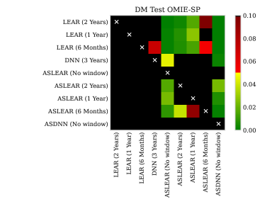
Figure 13: Multivariate DM test between each analyzed model for the OMIE-SP market

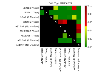
Figure 14: Multivariate DM test between each analyzed model for the EPEX-DE market

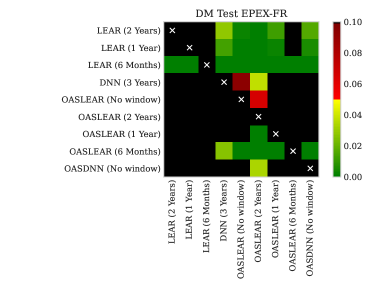
Figure 15: Multivariate DM test between each analyzed model for the EPEX-FR market (with the effect of the outliers mitigated)

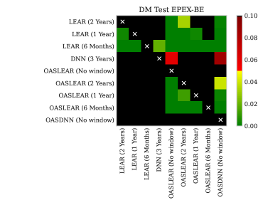
Figure 16: Multivariate DM test between each analyzed model for the EPEX-BE market (with the effect of the outliers mitigated)

It can be observed that in all markets except for the Belgian market, there is at least one adaptive version of the model that statistically outperforms the non-adaptive versions with a p-value threshold of 0.05. With a threshold of 0.10, this holds true even for the Belgian market. There is no case where a non-adaptive version achieves superior performance compared to the adaptive versions, in terms of statistical significance. Furthermore, these results hold consistently for both the LEAR and DNN models. This is, if we compare the (O)ASLEAR (No window) with all LEAR type models, we have statistical evidence of improvement for all markets with a threshold of 0.05. If we compare the (O)ASDNN with the DNN, for the OMIE-SP and EPEX-DE markets we have statistical evidence with the same threshold. With a threshold of 0.10 there is also a meaningful statistical improvement for the Belgian case and no statistical improvement is observed for the French case. Looking at the performance by month in Figure 11 there are some periods with clear improvements by using the OASDNN model. However, there are some months with slight decrease in performance, which leads to this result in the statistical test.

Additionally, the use of all available data for model training without the use of windows generally leads to better results, which is not always the case for the non adaptive models. This confirms the previous assertion that the effects of changes accumulate in $\mu_{d}$ and $\sigma_{d}$. Moreover, among the adaptive models without windows, there is no statistically significant evidence to support the superiority of one model over another. This indicates that the modeling approach for $f$ in Equation (1) is equally valid based on the results obtained.

5 Conclusions

In this work, a new framework for a price prediction model in the Day-Ahead market based on the price dynamics has been proposed. This new approach has been thoroughly studied, demonstrating improved results across various metrics and showing statistical improvement in four different markets and two distinct market periods. The outlier mitigation process has proven to be vital for achieving these results. Additionally, two new and recent datasets have been made available to the community, aiming to explore new models on datasets that are closer to the current market situation.

While the results may be further improved by using alternative learning algorithms for $f$ in Equation (1), no statistically significant difference has been observed among the evaluated models in this study. One way to achieve better results could be through the use of additional explanatory variables in estimating $\mu_{d}$ and $\sigma_{d}$. In fact, adaptive standardisation has been used, but other adaptive transformations could also be considered. The inclusion of new explanatory features, especially those related to variable generation costs such as gas prices, oil prices, etc., can lead to improved results (Ortiz et al., 2016; Marcjasz et al., 2023; Shiri et al., 2015). In this context where frequent changes in data distribution can occur, the selection of variables must be done carefully (Sebastián and González-Guillén, 2023). It is crucial to consider the potential impact of dataset shifts and the biases that can be generated in this context by different explanatory variables. Additionally, we advocate for the incorporation of dynamic performance measures in the literature. These measures provide a deeper insight into the behavior of models, allowing for a more comprehensive understanding of their performance. They also simplify the assessment of situations where models may fall short in delivering accurate predictions.

Declaration of competing interest

The authors declare that they have no known competing financial interests or personal relationships that could have appeared to influence the work reported in this paper.

CRediT authorship contribution statement

Carlos Sebastián: Writing – original draft, Visualization, Software, Methodology, Conceptualization. Carlos E. González-Guillén: Writing – review & editing, Validation, Supervision, Conceptualization, Project administration, Funding acquisition. Jesús Juan: Writing – review & editing, Validation, Supervision, Conceptualization, Project administration, Funding acquisition.

Data availability

The authors have shared the link to the repository, where the data and the code to reproduce the results are available.

Funding

This work has been funded by grant MIG-20211033 from Centro para el Desarrollo Tecnológico Industrial, Ministerio de Universidades, and European Union-NextGenerationEU. C.E.G.G. was also funded by a Re-qualification grant of Universidad Politécnica de Madrid funded by European Union-NextGenerationEU and by Ministerio de Universidades.

Appendix A Outlier mitigation

To reduce the sensitivity of the model to outlier observations, an outlier detection process is implemented. Any outlier observation in the intervened target time series will be seen as a “normal” observation. This is accomplished by following a simple logic. Let $\Delta_{d}^{h}$ denote the difference between the price at day $d$ and hour $h$ and the price 24 hours earlier. This is

$$\Delta_{d}^{h}=p_{d}^{h}-p_{d-1}^{h}$$

We will work with a fixed proportion of observations as outliers, denoted by $\alpha$, which in practice will be $\alpha=0.05$. To identify these outliers, we calculate the quantiles $1-\frac{\alpha}{2}$ and $\frac{\alpha}{2}$ of $\Delta_{d}^{h}$. We denote these quantiles as $q(\Delta,1-\frac{\alpha}{2})$ and $q(\Delta,\frac{\alpha}{2})$, respectively, where $\Delta$ is the vector containing every $\Delta_{d}^{h}$ computed.

Any observation that satisfies $\Delta_{d}^{h}>q(\Delta,1-\frac{\alpha}{2})$ or $\Delta_{d}^{h}<q(\Delta,\frac{\alpha}{2})$ will be defined as an outlier. The transformed target series is then defined as follows:

$${\tilde{p}_{d}^{h}}=\begin{cases}p_{d}^{h}\;&\text{if the observation is not an outlier}\\ q(\textbf{P}_{d}^{h},0.5)\;&\text{if the observation is an outlier}\end{cases}$$

where $\textbf{P}_{d}^{h}=\left(p_{d-1}^{h},p_{d-2}^{h},\dots,p_{d-7}^{h}\right)^{T}$.

For instance, the original and transformed Day-Ahead prices of the EPEX-BE market can be seen in Figure 17. The attenuation of price spikes can be easily observed.

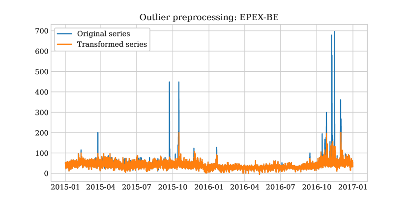
Figure 17: Comparison between the transformed (without outliers) and the original price series of the EPEX-BE Day-Ahead market

References

- Bergstra et al. (2011) Bergstra, J., Bardenet, R., Bengio, Y., Kégl, B., 2011. Algorithms for hyper-parameter optimization. Advances in neural information processing systems 24.
- Chen et al. (2021) Chen, Y., Koch, T., Lim, K.G., Xu, X., Zakiyeva, N., 2021. A review study of functional autoregressive models with application to energy forecasting. Wiley Interdisciplinary Reviews: Computational Statistics 13, e1525.
- Chen and Li (2017) Chen, Y., Li, B., 2017. An adaptive functional autoregressive forecast model to predict electricity price curves. Journal of Business & Economic Statistics 35, 371–388.
- Diebold and Mariano (2002) Diebold, F.X., Mariano, R.S., 2002. Comparing predictive accuracy. Journal of Business & economic statistics 20, 134–144.
- Efron (1992) Efron, B., 1992. Bootstrap methods: another look at the jackknife. Springer.
- Gamakumara et al. (2023) Gamakumara, P., Santos-Fernandez, E., Talagala, P.D., Hyndman, R.J., Mengersen, K., Leigh, C., 2023. Conditional normalization in time series analysis. arXiv preprint arXiv:2305.12651 .
- Giacomini and White (2006) Giacomini, R., White, H., 2006. Tests of conditional predictive ability. Econometrica 74, 1545–1578.
- Harris and Sollis (2003) Harris, R., Sollis, R., 2003. Applied time series modelling and forecasting. Wiley.
- Hastie and Tibshirani (1990) Hastie, T., Tibshirani, R., 1990. Generalized Additive Models. Chapman & Hall/CRC Monographs on Statistics & Applied Probability, Taylor & Francis.
- Hong et al. (2020) Hong, T., Pinson, P., Wang, Y., Weron, R., Yang, D., Zareipour, H., 2020. Energy forecasting: A review and outlook. IEEE Open Access Journal of Power and Energy 7, 376–388.
- Jan et al. (2022) Jan, F., Shah, I., Ali, S., 2022. Short-term electricity prices forecasting using functional time series analysis. Energies 15, 3423.
- Kath and Ziel (2021) Kath, C., Ziel, F., 2021. Conformal prediction interval estimation and applications to day-ahead and intraday power markets. International Journal of Forecasting 37, 777–799.
- Kingma and Ba (2014) Kingma, D.P., Ba, J., 2014. Adam: A method for stochastic optimization. arXiv preprint arXiv:1412.6980 .
- Koenker and Bassett Jr (1978) Koenker, R., Bassett Jr, G., 1978. Regression quantiles. Econometrica: journal of the Econometric Society , 33–50.
- Kupiec et al. (1995) Kupiec, P.H., et al., 1995. Techniques for verifying the accuracy of risk measurement models. volume 95-24. Division of Research and Statistics, Division of Monetary Affairs, Federal Reserve Board.
- Lago et al. (2018) Lago, J., De Ridder, F., De Schutter, B., 2018. Forecasting spot electricity prices: Deep learning approaches and empirical comparison of traditional algorithms. Applied Energy 221, 386–405.
- Lago et al. (2021) Lago, J., Marcjasz, G., De Schutter, B., Weron, R., 2021. Forecasting day-ahead electricity prices: A review of state-of-the-art algorithms, best practices and an open-access benchmark. Applied Energy 293, 116983.
- Marcjasz et al. (2023) Marcjasz, G., Narajewski, M., Weron, R., Ziel, F., 2023. Distributional neural networks for electricity price forecasting. Energy Economics 125, 106843.
- Mashlakov et al. (2021) Mashlakov, A., Kuronen, T., Lensu, L., Kaarna, A., Honkapuro, S., 2021. Assessing the performance of deep learning models for multivariate probabilistic energy forecasting. Applied Energy 285, 116405.
- Narajewski and Ziel (2021) Narajewski, M., Ziel, F., 2021. Optimal bidding on hourly and quarter-hourly day-ahead electricity price auctions: trading large volumes of power with market impact and transaction costs. arXiv preprint arXiv:2104.14204 .
- Nasiadka et al. (2022) Nasiadka, J., Nitka, W., Weron, R., 2022. Calibration window selection based on change-point detection for forecasting electricity prices, in: Computational Science–ICCS 2022: 22nd International Conference, London, UK, June 21–23, 2022, Proceedings, Part III, Springer. pp. 278–284.
- Nowotarski and Weron (2015) Nowotarski, J., Weron, R., 2015. Computing electricity spot price prediction intervals using quantile regression and forecast averaging. Computational Statistics 30, 791–803.
- Ogasawara et al. (2010) Ogasawara, E., Martinez, L.C., De Oliveira, D., Zimbrão, G., Pappa, G.L., Mattoso, M., 2010. Adaptive normalization: A novel data normalization approach for non-stationary time series, in: The 2010 International Joint Conference on Neural Networks (IJCNN), IEEE. pp. 1–8.
- Olivares et al. (2023) Olivares, K.G., Challu, C., Marcjasz, G., Weron, R., Dubrawski, A., 2023. Neural basis expansion analysis with exogenous variables: Forecasting electricity prices with nbeatsx. International Journal of Forecasting 39, 884–900.
- Oreshkin et al. (2019) Oreshkin, B.N., Carpov, D., Chapados, N., Bengio, Y., 2019. N-beats: Neural basis expansion analysis for interpretable time series forecasting. arXiv preprint arXiv:1905.10437 .
- Ortiz et al. (2016) Ortiz, M., Ukar, O., Azevedo, F., Múgica, A., 2016. Price forecasting and validation in the spanish electricity market using forecasts as input data. International Journal of Electrical Power & Energy Systems 77, 123–127.
- Passalis et al. (2019) Passalis, N., Tefas, A., Kanniainen, J., Gabbouj, M., Iosifidis, A., 2019. Deep adaptive input normalization for time series forecasting. IEEE transactions on neural networks and learning systems 31, 3760–3765.
- Quiñonero-Candela et al. (2008) Quiñonero-Candela, J., Sugiyama, M., Schwaighofer, A., Lawrence, N.D., 2008. Dataset shift in machine learning. Mit Press, Cambridge, Massachusetts.
- Sebastián and González-Guillén (2023) Sebastián, C., González-Guillén, C.E., 2023. A feature selection method based on shapley values robust to concept shift in regression. arXiv preprint arXiv:2304.14774 .
- Shiri et al. (2015) Shiri, A., Afshar, M., Rahimi-Kian, A., Maham, B., 2015. Electricity price forecasting using support vector machines by considering oil and natural gas price impacts, in: 2015 IEEE international conference on smart energy grid engineering (SEGE), IEEE. pp. 1–5.
- Uniejewski et al. (2016) Uniejewski, B., Nowotarski, J., Weron, R., 2016. Automated variable selection and shrinkage for day-ahead electricity price forecasting. Energies 9, 621.
- Uniejewski and Weron (2018) Uniejewski, B., Weron, R., 2018. Efficient forecasting of electricity spot prices with expert and lasso models. Energies 11, 2039.
- Uniejewski and Weron (2021) Uniejewski, B., Weron, R., 2021. Regularized quantile regression averaging for probabilistic electricity price forecasting. Energy Economics 95, 105121.
- Uniejewski et al. (2017) Uniejewski, B., Weron, R., Ziel, F., 2017. Variance stabilizing transformations for electricity spot price forecasting. IEEE Transactions on Power Systems 33, 2219–2229.
- Vovk et al. (2005) Vovk, V., Gammerman, A., Shafer, G., 2005. Algorithmic learning in a random world. volume 29. Springer.
- Ziel and Steinert (2016) Ziel, F., Steinert, R., 2016. Electricity price forecasting using sale and purchase curves: The x-model. Energy Economics 59, 435–454.
- Ziel and Weron (2018) Ziel, F., Weron, R., 2018. Day-ahead electricity price forecasting with high-dimensional structures: Univariate vs. multivariate modeling frameworks. Energy Economics 70, 396–420.