Physics-informed dynamic mode decomposition for short-term and long-term prediction of gas-solid flows

Abstract

Integration of physics principles with data-driven methods has attracted great attention in recent few years. In this study, a physics-informed dynamic mode decomposition (piDMD) method, where the mass conservation law is integrated with a purely data-driven DMD method, is developed for fast prediction of the spatiotemporal dynamics of solid volume fraction distribution in bubbling fluidized beds. Assessment of the prediction ability using both piDMD and DMD is performed using the CFD-DEM results as the benchmark: Both DMD and piDMD can predict the short-term behaviour of solid volume fraction reasonably well, but piDMD outperforms the DMD in both qualitative and quantitative comparisons; With respect to their long-term ability, the piDMD-based prediction of the instantaneous solid volume fraction distributions is qualitatively correct although the accuracy needs to be improved, and the predicted time-averaged radial and axial profiles are satisfactory; Whereas the DMD-based prediction of instantaneous snapshots and time-averaged results is completely nonphysical. Present study provides a fast and relatively accurate method for predicting the hydrodynamics of gas-solid flows.

1 Introduction

Gas-solid flows are widely encountered in industry and in nature (Wang, 2020). For example, fluidization technology is one of the most important and widely-used technologies in industrial processes, such as the fluid catalytic cracking, the calcination of ores, the polymerization of olefins, the combustion of coal, municipal waste, and biomass (Fan, 1996). In recent decades, computational multiphase fluid dynamics has been a pivotal and fast-growing research focus of chemical engineering field (van der Hoef et al., 2006; Ge et al., 2019a; Zhang et al., 2023), one of its major expectations is that the design, optimized operation, scale-up, and dynamic control of chemical reactors can be carried out digitally, without laborious and expensive experiments. For instance, the concept of virtual process engineering have been proposed in recent years to replace the traditional trial-and-error strategy of reactor design and scale-up (Ge et al., 2011, 2019b), which has put forward an extremely high demand on the accuracy and speed of computational fluid dynamics (CFD) simulations. Clearly, the dream of chemical engineers is fully in line with the broader effort in the development of the most promising and enabling digital twin technology for realizing smart manufacturing and Industry 4.0 (Tao et al., 2018; Jones et al., 2020; Baranidharan et al., 2022).

One of the critical steps towards the realization of digital twin of chemical reactors is the capability of simulating and predicting chemical reactors accurately and quickly, including the fluidized bed reactor studied in present article. Various approaches have been developed for fast simulation and/or prediction of gas-solid flows in fluidized bed reactors, such as recurrence CFD (Lichtenegger and Pirker, 2016; Lichtenegger, 2018; Dabbagh et al., 2021), deep learning (Zhang et al., 2020b; Bazai et al., 2021; Faridi et al., 2023; Qin et al., 2023; Wen et al., 2023), GPU-based computation (Xu et al., 2011, 2022) and reduced-order model (Yuan et al., 2005; Yu et al., 2015; Zhong et al., 2020; Yu et al., 2021; Li et al., 2022a; Hajisharifi et al., 2023). For example, for the prediction of solid phase volume fraction distribution in gas-solid fluidized beds, Bazai et al. (2021) trained a convolutional neural network (CNN) using CFD data, the trained CNN model predicts the next time-step solid volume fraction distribution quicker than the CFD simulation, however, the long-term prediction using the proposed CNN requires constant inputs of CFD data in order not to lose its accuracy; Qin et al. (2023) presented a new approach of deep learning for voidage prediction.

With the successful application of data-driven methods in extraction of coherent structures and reconstruction of flow field for gas-solid systems (Cizmas et al., 2003; Haghgoo et al., 2019; Higham et al., 2020; Li et al., 2022b, 2023), recent developments in data-driven methods have found potentials in simulating complex fluid motion for computational acceleration and fast prediction (Curtis and Alford-Lago, 2021; Ghadami and Epureanu, 2022; Baddoo et al., 2023). In order to predict gas-solid fluidized beds efficiently, this study develops a physics-informed dynamic mode decomposition (piDMD) method, which combines the data-driven approach with the mass conservation law, to predict the solid phase volume fraction of a bubbling fluidized bed. The remaining sections of the article are: Section 2 introduces the piDMD method; Section 3 is an introduction to the CFD-DEM method; Section 4 analyses and discusses the results; and Section 5 is a summary and outlook of present article.

2 Physics-informed Dynamic mode decomposition

The DMD method (Rowley et al., 2009; Schmid, 2010, 2022) is a powerful mathematical tool, which uses the infinite dimensional linear Koopman operator to analyze the nonlinear behaviour in finite dimensions (Mezić, 2013; Brunton et al., 2021). Collecting data from a series of time snapshots of the flow field is the first step of DMD. As illustrated on the left side of Fig.1, a snapshot obtained from numerical simulation corresponds to a vector in data analysis. The specific task of data collection is to arrange the data of each snapshot into a vector according to a fixed sequence of spatial location (grid position), the resulting vectors are then further sorted to obtain the snapshot matrix according to time series. Assuming that $\mathbf{z}_{i}$ is the vector composed of a snapshot at the $i$th time, and vectors at different time steps are ordered chronologically to form two snapshot matrices $\mathbf{Z}_{0}$ and $\mathbf{Z}_{1}$ that differ by unit time step as shown below,

$$\begin{split}&{{\bf{Z}}_{0}}=\left[{\begin{array}[]{*{20}{c}}{\begin{array}[]{*{20}{c}}{\rm{|}}\\ {{{\bf{z}}_{0}}}\\ {\rm{|}}\end{array}}&{\begin{array}[]{*{20}{c}}{\rm{|}}\\ {{{\bf{z}}_{1}}}\\ {\rm{|}}\end{array}}&{\begin{array}[]{*{20}{c}}{\rm{|}}\\ \cdots\\ {\rm{|}}\end{array}}&{\begin{array}[]{*{20}{c}}{\rm{|}}\\ {{{\bf{z}}_{M-1}}}\\ {\rm{|}}\end{array}}\end{array}}\right],\\ &{{\bf{Z}}_{1}}=\left[{\begin{array}[]{*{20}{c}}{\begin{array}[]{*{20}{c}}{\rm{|}}\\ {{{\bf{z}}_{1}}}\\ {\rm{|}}\end{array}}&{\begin{array}[]{*{20}{c}}{\rm{|}}\\ {{{\bf{z}}_{2}}}\\ {\rm{|}}\end{array}}&{\begin{array}[]{*{20}{c}}{\rm{|}}\\ \cdots\\ {\rm{|}}\end{array}}&{\begin{array}[]{*{20}{c}}{\rm{|}}\\ {{{\bf{z}}_{M}}}\\ {\rm{|}}\end{array}}\end{array}}\right],\\ &{\mathbf{Z}_{0}},\;{\mathbf{Z}_{1}}\in{R^{N\times M}},\end{split}$$ (1)

where $M+1$ is the total number of snapshots, and $N$ is the number of spatial locations or the number of computational cells. The underlying linearity assumption of the DMD method is

$${\mathbf{z}_{i+1}}=\mathbf{A}{\mathbf{z}_{i}},$$ (2)

whose rollout to a sequential set of snapshots is ${\mathbf{Z}}_{1}=\mathbf{A}{\mathbf{Z}}_{0}$. DMD aims to make $\mathbf{A}$ an optimal low-rank approximation matrix as a DMD operator to approximate the dynamical process in the nonlinear dynamical system. The DMD regression, whose minimization is phrased in the Frobenius norm, is formulated as

$$\mathop{\arg\min}\limits_{{\rm{rank}}\left({\bf{A}}\right)=r}{\left\|{{{\bf{Z}}_{1}}-{\bf{A}}{{\bf{Z}}_{0}}}\right\|_{F}}.$$ (3)

Finding the optimal $\mathbf{A}$ that satisfies Eq. 3 is the key to the DMD process. The standard DMD algorithm for prediction is based on the singular value decomposition (SVD) (Stewart, 1993) to solve Eq. 3. SVD decomposes any matrix into the multiplication of three matrices, i.e. an orthogonal matrix $\bf{U}$ composed of left singular vectors, a diagonal matrix $\bf{\Sigma}$, and an orthogonal matrix ${\bf{V}}^{*}$ composed of right singular vectors, an example is ${{\bf{Z}}_{0}}={\bf{U\Sigma}}{{\bf{V}}^{*}}$. SVD is obtained by conventional matrix operations and is easy to implement in the programming language. The contribution of SVD to the DMD-based prediction is to transform the matrix ${\bf{Z}}_{0}$ that cannot be inverted into three square matrices ($\bf{U}$, ${\bf{\Sigma}}$, and ${\bf{V}}$) that can be inverted. The specific process of DMD-based prediction of solid phase volume fraction is as follows (Schmid, 2010; Tu, 2013):

${1.}$ Obtain two snapshot matrices $\mathbf{Z}_{0}$ and $\mathbf{Z}_{1}$ from Eq. 1.

${2.}$ Compute the SVD of ${{\bf{Z}}_{0}}$,

$${{\bf{Z}}_{0}}={\bf{U\Sigma}}{{\bf{V}}^{*}}.$$ (4)

${3.}$ Calculate the high-dimensional mapping matrix $\mathbf{A}$ using the following equation,

$${\bf{A}}={{\bf{Z}}_{1}}{{{\bf{Z}}_{0}}^{\dagger}}={{\bf{Z}}_{1}}{\bf{V}}{{\bf{\Sigma}}^{-1}}{{\bf{U}}^{*}},$$ (5)

where $(\cdot)^{\dagger}$ represents a pseudoinverse operation and $(\cdot)^{-1}$ represents an inverse operation.

${4.}$ By using the obtained $\mathbf{A}$ and the solid volume fraction of the flow field at the $j$th time, which is expressed as $\mathbf{z}_{j}$, the solid volume fraction of the flow field at the $j+1$th time, which is expressed as $\mathbf{z}_{j+1}$, can then be predicted using the formula as

$${\mathbf{z}_{j+1}}=\mathbf{A}{\mathbf{z}_{j}}.$$ (6)

Then the DMD-based prediction of solid volume fraction at the next moment only requires repeating step $4$.

The DMD method is a purely data-driven method, which cannot automatically satisfy the known physical laws of studied systems. In order to remedy this deficiency, physics-informed dynamic mode decomposition (piDMD) has been proposed recently (Baddoo et al., 2023). The piDMD method is based on the purely data-driven DMD method with the addition of the underlying physical laws of the system as constraints, so systems with different physical laws correspond to different piDMD methods. Via analyzing the system characteristics of gas-solid bubbling fluidized beds, i.e. the sum of solid phase volume fraction at any moments is conserved or the mass of solid phase is conserved, a piDMD method that satisfies the mass conservation law is developed in present study. Fig.1 illustrates the concept of and the implementation procedure of piDMD for analyzing the coherent structures from the snapshots of solid volume fraction obtained from CFD-DEM simulation of gas-solid flows and then predicting the spatiotemporal dynamics of solid volume fraction.

The mathematical difference between DMD and piDMD is the calculation of the high-dimensional mapping matrix $\mathbf{A}$. It is clear that the bubbling bed in this study is characterized by the conservation of the sum of solid volume fractions, supposing that $\mathbf{z}_{i}$ represents the snapshot of solid volume fraction at the $i$th time, and the conservation of the sum of solid volume fraction is expressed mathematically as

$${\left\|{{{\bf{z}}_{i+1}}}\right\|_{1}}={\left\|{{{\bf{z}}_{i}}}\right\|_{1}},$$ (7)

where the operator ${\left\|\cdot\right\|_{1}}$ denotes the 1-norm, and the 1-norm value of a vector is the sum of absolute value of each element of the vector. It is difficult to find a numerical solution for the coupling of the 1-norm with the DMD method. But if you take the square root of each element in the snapshot vector and then square them, the resulting sum will be equal to the sum of the absolute values of each element in the vector. Thus, the modified vector’s 2-norm can be calculated with its elements set as the square root of each cell’s solid concentration (i.e. $\left\|{{{\bf{z}}_{i,new}}}\right\|_{2}^{2}={\left\|{{{\bf{z}}_{i}}}\right\|_{1}}$). This altered 2-norm (Eq.8) is equal to the original hydrodynamic solid concentration field’s 1-norm (Eq.7)

$$\left\|{{{\bf{z}}_{i+1,new}}}\right\|_{2}^{2}=\left\|{{{\bf{z}}_{i,new}}}\right\|_{2}^{2}.$$ (8)

Substitute Eq. 2 into Eq. 8 as

$${\left\|{{\bf{A}}{{\bf{z}}_{i,new}}}\right\|_{2}^{2}=\left\|{{{\bf{z}}_{i,new}}}\right\|_{2}^{2}.}$$ (9)

In matrix terminology, Eq.9 holds if and only if $\mathbf{A}$ is unitary ($\mathbf{A}^{*}\mathbf{A}=\mathbf{I}$) (Schönemann, 1966). The feature that $\mathbf{A}$ is a unitary matrix ensures the physical law of mass conservation and serves as a constraint on the DMD regression, which constitutes the piDMD method in this study. Therefore, the piDMD regression is (Baddoo et al., 2023)

$$\arg\min{\left\|{{{\bf{Z}}_{1,new}}-{\bf{A}}{{\bf{Z}}_{0,new}}}\right\|_{F}},\,s.t.\,\mathbf{A}^{*}\mathbf{A}=\mathbf{I}.$$ (10)

The executable approach of piDMD-based prediction of solid volume fraction is summarized in Algorithm 1, steps $1$ and $5$ are exactly the same as DMD-based prediction, and steps $3$ and $4$ are the analytical solution process (Schönemann, 1966) for the piDMD regression. Predicting the solid volume fractions of the flow field at the next moment only requires repeating steps $5$ and $6$ in Algorithm 1.

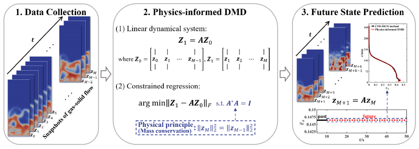
Figure 1: Illustration of prediction of dense gas-solid flow using physics-informed dynamic mode decomposition (piDMD). ${I}$ is the identity matrix, the operators $(\cdot)^{*}$, ${\left\|\cdot\right\|_{F}}$, and ${\left\|\cdot\right\|_{2}}$ denote the conjugate transpose operation, the Frobenius norm, and the 2-norm.

Table 1:

Algorithm 1: piDMD-based prediction of solid volume fraction

${1.}$ Obtain two snapshot matrices $\mathbf{Z}_{0}$ and $\mathbf{Z}_{1}$ from Eq. 1.

${2.}$ Take the square root of each element of the matrix $\mathbf{Z}_{0}$ and $\mathbf{Z}_{1}$ to form ${\bf{Z}}_{0,new}$ and ${\bf{Z}}_{1,new}$.

${3.}$ Compute the SVD of ${{\bf{Z}}_{1,new}}{{\bf{Z}}_{0,new}^{*}}$,

${{\bf{Z}}_{1,new}}{{\bf{Z}}_{0,new}^{*}}={{\bf{U}}_{new}}{{\bf{\Sigma}}_{new}}{{\bf{V}}_{new}^{*}}$.

${4.}$ Calculate the high-dimensional mapping matrix $\mathbf{A}$ of the piDMD method with Eq. 10,

${\bf{A}}={{\bf{U}}_{new}}{{{\bf{V}}_{new}^{*}}}$.

${5.}$ Predict $\mathbf{z}_{j+1,new}$ using ${\mathbf{z}_{j+1,new}}=\mathbf{A}{\mathbf{z}_{j,new}}$.

${6.}$ Take the square of each element of $\mathbf{z}_{j+1,new}$ to obtain the solid volume fractions at the $j+1$th time, $\mathbf{z}_{j+1}$.

3 CFD-DEM method

As mentioned earlier, the input data $\mathbf{Z}_{0}$ and $\mathbf{Z}_{1}$ for the DMD-based and piDMD-based analysis and prediction come from the computer simulation of a bubbling fluidized bed using CFD-DEM method. However, it should be emphasized that the input data are not limited to CFD-DEM simulations, they can also be obtained from any other simulations where field variables of solid volume fraction are available, such as two-fluid model (TFM) (Gidaspow, 1994; Wang, 2020) and dynamic multiscale method (Chen and Wang, 2017, 2018). CFD-DEM method (Tsuji et al., 1993; van der Hoef et al., 2006) is one of the mainstream methods for numerical simulation of dense gas-solid systems. Table 2 summarizes the main equations of the CFD-DEM method used in present study. Specifically, the volume-averaged Navier-Stokes equations of gas phase are solved in the Eulerian framework using the open-source software OpenFOAM^® (Holzmann, 2016); the Newton’s second law is applied in the Lagrangian framework to obtain the movement of individual solid particle (van der Hoef et al., 2006; Golshan et al., 2020; Kieckhefen et al., 2020), which is solved using the in-house GPU-based DEMms (discrete element method for multiscale simulation) software (Xu et al., 2011; Lu et al., 2014; Xu et al., 2022). This coupled software has successfully simulated the hydrodynamics, heat, mass transfer, and chemical reactions in various fluidized beds (Lu et al., 2014, 2016; Zhang et al., 2017; Xu et al., 2019; Zhang et al., 2019; Lan et al., 2020; Liu et al., 2020; Zhang et al., 2020a; Zhao et al., 2020a, b, 2022a, 2022b; Lu et al., 2023). Therefore, the CFD-DEM data are directly used for piDMD and DMD analysis and as the benchmark for evaluating the short-term and long-term prediction of piDMD and DMD, without any further experimental validations.

CFD-DEM simulation of a typical bubbling fluidized bed is carried out, where the required physical parameters and numerical settings are reported in Table 3. There are only air and solid particles in this bubbling fluidized bed, and its motion is such that air enters uniformly from the bottom of the bed and exits from the top, and the stationary piled-up spherical particles form a fluidized state under the action of air. During the period of steady fluidization, there are continuous generation, growth, coalescence and breakup of bubbles in the fluidized bed.

Table 2: Main equations of CFD-DEM method

Equations of translational motion of particle:

$m_{a}\frac{d^{2}{\bf r}_{a}}{dt^{2}}=-V_{a}\nabla p+\frac{V_{a}\beta}{1-\varepsilon_{g}}({\bf u}_{g}-{\bf v}_{a})+{m_{a}}{\bf g}$

$+\sum_{b\in\text{contactlist }}\left(\mathbf{F}_{ba,n}+\mathbf{F}_{ba,t}\right)$

Equations of rotational motion of particle:

$I_{a}\frac{d\omega_{a}}{dt}=\mathbf{T}_{a}\text{, where }I_{a}=\frac{2}{5}m_{a}R_{a}^{2}$

Torque of particle:

$\mathbf{T}_{a}=\sum_{b\in\text{contactlist }}\left(R_{a}\mathbf{n}_{ab}\times\mathbf{F}_{ba,t}\right)$

Normal contact force between two particles:

$\mathbf{F}_{ba,n}=-k_{n}\delta_{n}\mathbf{n}_{ab}-\eta_{n}\mathbf{v}_{ba,n},$

where $\delta_{n}=d_{p}-\left|\mathbf{r}_{b}-\mathbf{r}_{a}\right|$, $\eta_{n}=\frac{-2\operatorname{\ln e}\sqrt{k_{n}m^{*}}}{\sqrt{(\pi)^{2}+(\ln e)^{2}}}$

Tangential contact force between two particles:

$\mathbf{F}_{ba,t}=\left\{\begin{array}[]{cc}-\eta_{t}\mathbf{v}_{ba,t}&\left|\mathbf{F}_{ba,t}\right|\leqslant\mu_{f}\left|\mathbf{F}_{ba,n}\right|\\ -\mu_{f}\left|\mathbf{F}_{ba,n}\right|\mathbf{t}_{ba}&\left|\mathbf{F}_{ba,t}\right|>\mu_{f}\left|\mathbf{F}_{ba,n}\right|\end{array}\right.$

where $\mathbf{v}_{ba,t}=\mathbf{v}_{ba}-\mathbf{v}_{ba,n},\eta_{t}=\eta_{n},\mathbf{t}_{ba}=\frac{\mathbf{v}_{ba,t}}{\left|\mathbf{v}_{ba,t}\right|}$

Solid phase volume fraction of grid A:

${\varepsilon_{\mathrm{p},\mathrm{A}}=\frac{{\sum\nolimits_{\mathrm{p}}{{{\mathrm{V}}_{\mathrm{p}}}}}}{{{{\mathrm{V}}_{\mathrm{A}}}}}}.$

Grid-averaged particle velocity of grid $A$:

$\mathbf{u}_{\mathrm{p},\mathrm{A}}=\left\{\begin{array}[]{l}\frac{\sum_{\mathrm{p}}\left(V_{\mathrm{p}}m_{\mathrm{p}}\mathbf{u}_{\mathrm{p}}g\left(\left|\mathbf{r}_{\mathrm{p}}-\mathbf{x}_{\mathrm{A}}\right|/h\right)\right)}{\sum_{\mathrm{p}}\left(V_{\mathrm{p}}m_{\mathrm{p}}g\left(\left|\mathbf{r}_{\mathrm{p}}-\mathbf{x}_{\mathrm{A}}\right|/h\right)\right)},V_{\mathrm{A}}<v_{\mathrm{cs}}^{3}\\ \frac{\sum_{\mathrm{p}}m_{\mathrm{p}}V_{\mathrm{p}}}{m_{\mathrm{p}}},V_{\mathrm{A}}\geq v_{\mathrm{cs}}^{3}\end{array}\right.$

Gas-solid drag coefficient of grid A:

$K_{\mathrm{gp},\mathrm{A}}=\left\{\begin{array}[]{l}\frac{\sum_{\mathrm{p}}\left(\beta V_{\mathrm{p}}\left|\mathbf{u}_{g,\mathrm{A}}-\mathbf{v}_{\mathrm{p}}\right|g\left(\left|\mathbf{r}_{\mathrm{p}}-\mathbf{x}_{\mathrm{A}}\right|/h\right)/\varepsilon_{\mathrm{p},\mathrm{A}}\right)}{\left|\mathbf{u}_{g,\mathrm{A}}-\mathbf{v}_{\mathrm{p}}\right|\sum_{c=1}^{N_{\mathrm{grid}}}\left(g\left(\left|\mathbf{x}_{c}-\mathbf{x}_{\mathrm{A}}\right|/h\right)\right)},V_{\mathrm{A}}<v_{\mathrm{cs}}^{3}\\ \frac{\sum_{\mathrm{p}}\left(\beta V_{\mathrm{p}}\left|\mathbf{u}_{\mathrm{g},\mathrm{A}}-\mathbf{v}_{\mathrm{p}}\right|/\varepsilon_{\mathrm{p},\mathrm{A}}\right)}{\left|\mathbf{u}_{\mathrm{g},\mathrm{A}}-\mathbf{v}_{\mathrm{p}}\right|V_{\mathrm{A}}},V_{\mathrm{A}}\geq v_{\mathrm{cs}}^{3}\end{array}\right.$

Gas phase mass conservation equation:

$\frac{\partial{(\varepsilon_{g}\rho_{g})}}{\partial t}+\nabla\cdot(\varepsilon_{g}\rho_{g}{\bf u}_{g})=0$

Gas phase momentum conservation equation:

$\frac{\partial{(\varepsilon_{g}\rho_{g}{\bf u}_{g})}}{\partial t}+\nabla\cdot(\varepsilon_{g}\rho_{g}{\bf u}_{g}{\bf u}_{g})=-\varepsilon_{g}\nabla p-{\bf S}_{p}$

$+\nabla\cdot(\varepsilon_{g}{\bf{\tau}}_{g})+\varepsilon_{g}\rho_{g}{\bf{g}}$

Gas-solid drag force density:

${\bf S}_{p}=\frac{1}{V_{cell}}\sum_{a=1}^{N_{part}}\frac{\beta V_{a}}{1-\varepsilon_{g}}({\bf u}_{g}-{\bf v}_{a})\delta({\bf r}-{\bf r}_{a}),$

where Gidaspow (Gidaspow, 1994) drag correlation is

$\beta=\left\{\begin{array}[]{cc}\frac{3}{4}C_{D}\frac{\rho_{g}\varepsilon_{g}\varepsilon_{s}\left|t\mathbf{u}_{g}-\mathbf{v}_{a}\right|}{d_{p}}\varepsilon_{g}^{-2.65}&\varepsilon_{g}>0.8\\ 150\frac{\varepsilon_{s}^{2}\mu_{g}}{\varepsilon_{g}d_{p}^{2}}+1.75\frac{\rho_{g}\varepsilon_{s}\left|t\mathbf{u}_{\mathrm{g}}-\mathbf{v}_{a}\right|}{d_{p}}&\varepsilon_{g}\leqslant 0.8\end{array}\right.$

with

$C_{D}=\left\{\begin{array}[]{cc}\frac{24}{Re}\left(1+0.15Re^{0.687}\right)&Re<1000\\ 0.44&Re\geqslant 1000\end{array}\right.$

and

$Re=\frac{\varepsilon_{g}\rho_{g}d_{p}|{\bf u}_{g}-{\bf v}_{a}|}{\mu_{g}}$

Gas phase stress-strain tensor:

${\bf{\tau}}_{g}=\mu_{g}(\nabla{\bf u}_{g}+\nabla{\bf u}_{g}^{T})-\frac{2}{3}\mu_{g}(\nabla\cdot{\bf u}_{g}){\bf I}$

Table 3: Physical and numerical parameters used in CFD-DEM simulation

Parameter	Value
Gas phase
Temperature, T (K)	298
Dynamic viscosity, $\mu$ (Pa s)	1.8$\times$$\/10^{-5}$
Inlet superficial gas velocity, u (m/s)	0.9
Minimum fluidization velocity, $u_{mf}$ (m/s)	0.3
Molecular weight, M (kg/mol)	$28.8\times 10^{-3}$
Pressure, p (atm)	1.0
Density, $\rho_{g}$ (kg/$\/m^{3}$)	1.2
CFD time step, dt (s)	1.0$\times 10^{-5}$
Particles
Number of particle	167490
Diameter, $\/d_{p}$ (m)	$1.2\times 10^{-3}$
Density, $\rho_{p}$ (kg/$\/m^{3}$)	1000
Normal spring stiffness, $\/k_{n}$ (N/m)	32
Tangential spring stiffness, $\/k_{t}$ (N/m)	32
Friction coefficient	0.1
Restitution coefficient, $\/e_{n},e_{t}$	0.97
Rolling friction coefficient	0.01
Particle dynamics time step (s)	$\/1.0\times{10^{{\rm{-}}5}}$
Geometry
Domain width, $x$ (m)	$0.1440$
Domain thickness, $y$ (m)	$0.0192$
Domain height, $z$ (m)	$0.3744$
Cell number, $\ {NX\times NY\times NZ}$	$30\times 4\times 78$
Grid length in the x-direction, $\Delta x$ (m)	$0.0048$
Grid length in the y-direction, $\Delta y$ (m)	$0.0048$
Grid length in the z-direction, $\Delta z$ (m)	$0.0048$

4 Result and discussion

DMD and piDMD analysis and prediction are performed using the $5001$ time snapshots with its sampling frequency of $1000\,$Hz, corresponding to the CFD-DEM result from $5\,$s to $10\,$s. Analysis of the differential pressure drop of the whole bubbling fluidized bed indicates that the dominant fluctuation frequencies are $2\sim 4\,$Hz (the results are not reported), furthermore, the sampling frequency of input data has a negligible effect on the prediction results provided that the data have contained sufficient information of bed dynamics, as shown in the Appendix. Therefore, only the results of a sampling frequency of $1000\,$Hz are reported here, which are analyzed and discussed in two parts: short-term prediction and long-term prediction.

4.1 Short-term Prediction

Short-term prediction includes $30$ snapshots of solid volume fraction ${\varepsilon_{s}}$, corresponding to the time range from $10.001\,$s to $10.030\,$s. Fig.2 visualizes the results of piDMD-based and DMD-based short-term predictions at same moments. It can be seen that both DMD and piDMD can predict the solid volume fraction reasonably well, but the piDMD predicted flow field is closer to the CFD-DEM predicted flow field than those of DMD predicted flow field, qualitatively indicating that piDMD-based short-term prediction is more accurate. Fig.3 shows a quantitative comparison of piDMD-based and DMD-based short-term predictions. Fig.3(a) illustrates the variation of simulation-domain-averaged solid phase volume fraction with time obtained from CFD-DEM simulation, piDMD-based short-term prediction, and DMD-based short-term prediction. The piDMD predicted and CFD-DEM simulated results are not only unchanged over time but also equal, whereas DMD predicted result follows a decreasing trend. The former observation indicates that the physical principle of mass conservation is faithfully satisfied, whereas the latter means the violation of the law of mass conservation since some mass is lost. The ratio of the 2-norm of the deviation of the predicted snapshot from the real snapshot to the 2-norm of the original snapshot is used as a quantitative criterion to assess the difference between the predicted flow field and CFD-DEM simulated flow field, which is given by

$$loss=\frac{{{{\left\|{{{\bf{z}}_{\rm{p}}}-{{\bf{z}}_{r}}}\right\|}_{2}}}}{{{{\left\|{{{\bf{z}}_{r}}}\right\|}_{2}}}}\times 100\%=\frac{{\sqrt{\sum\limits_{i=1}^{i=N}{{{\left({{z_{p,i}}-{z_{r,i}}}\right)}^{2}}}}}}{{\sqrt{\sum\limits_{i=1}^{i=N}{{z_{r,i}^{2}}}}}}\times 100\%,$$ (11)

where $\mathbf{z}_{p}$ is the vector composed of the predicted snapshot at a given time using either DMD or piDMD, and $z_{p,i}$ is its element. Similarly, $\mathbf{z}_{r}$ is the vector composed of the real snapshot at a given time obtained from CFD-DEM simulation, and $z_{r,i}$ is its element. The smaller $loss$ value indicates that the predicted flow field is closer to the real one. Fig.3(b) shows the $loss$ of the corresponding predicted flow field at each moment, and both curves show an increasing trend. However, the $loss$ of piDMD-based short-term prediction is smaller than that of DMD-based short-term prediction at each moment.

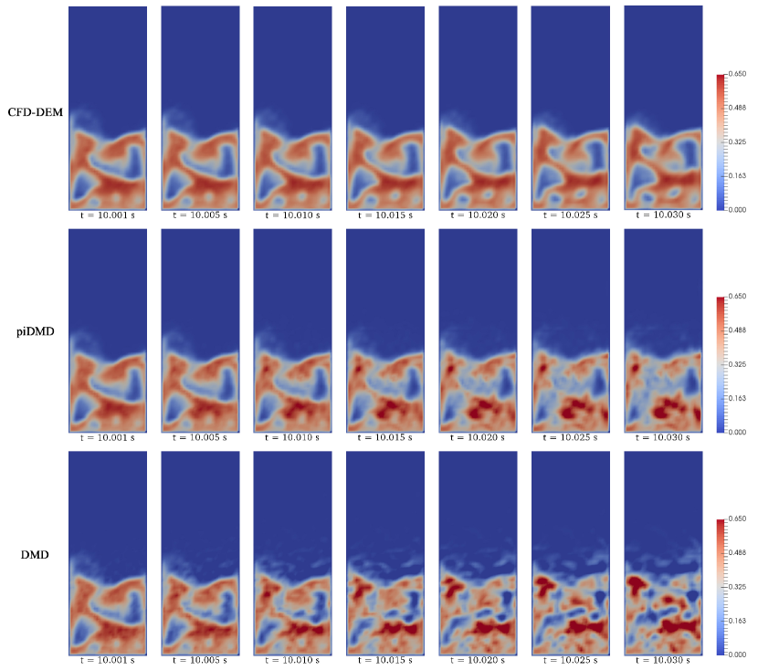
Figure 2: Snapshots of solid volume fraction obtained from CFD-DEM simulation, piDMD-based short-term prediction, and DMD-based short-term prediction.

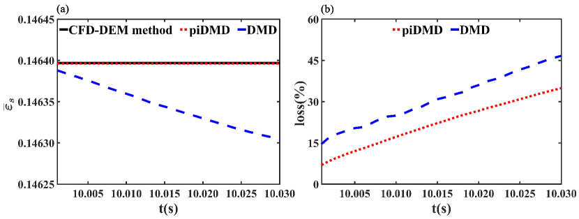
Figure 3: $(a)$ Simulation-domain-averaged solid phase volume fraction obtained from CFD-DEM simulation, piDMD-based short-term prediction, and DMD-based short-term prediction. $(b)$ The $loss$ obtained from piDMD-based short-term prediction and DMD-based short-term prediction.

The results in this section suggest that the piDMD method is effective in achieving the mass conservation law, but the purely data-driven DMD method results in the violation of mass conservation law, which is a reason for why the results of piDMD-based prediction are consistently better than those of DMD-based prediction.

4.2 Long-term Prediction

The time range for the long-term prediction is from $10\,$s to $50\,$s, and a total of $40001$ snapshots are predicted. As shown in Fig.4, by observing the difference in the color bar of CFD-DEM simulation, piDMD-based prediction, and DMD-based prediction at the physical time of $15\,$s, it is easy to find that the flow field predicted by the DMD method no longer possesses any physical reality of the flow field, but the flow field structure of piDMD-based prediction, although significantly different from that of CFD-DEM simulation, is still within the range of normal solid volume fraction values from a qualitative point of view.

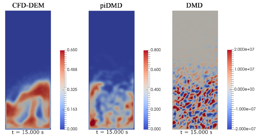
Figure 4: Snapshots of solid phase volume fraction at $t=15$ s, obtained from CFD-DEM simulation, piDMD-based prediction, and DMD-based prediction.

Fig.5(a) and (b) show the variation of simulation-domain-averaged solid volume fraction with time for CFD-DEM simulation and piDMD-based long-term prediction, and DMD-based long-term prediction, respectively. As can be seen from Fig.5(a), the piDMD-based long-term prediction keeps the mean solid volume fraction unchanged, which is also consistent with the CFD-DEM result. Fig.5(a) confirms that the piDMD predicted solid volume fraction strictly conforms to the physical law of mass conservation. Nevertheless, it can be found from Fig.5(b) that the mean solid volume fraction is not a fixed value, moreover, its fluctuation is increasing. The numerical range of the curve in Fig.5(b) is from $-10$ to $10$, which shows that the results of the DMD-based prediction are completely nonphysical, and the DMD method is unsuitable for long-term prediction of the hydrodynamics of bubbling fluidized beds. Fig.5(c) displays the loss of long-term prediction using the piDMD and DMD methods. It is found that the $loss$ curve of piDMD-based long-term prediction increases in the early stage and then reach an asymptotic value, whereas the $loss$ of DMD-based long-term prediction increases rapidly with time. From the subplot of Fig.5(c), it can be noticed that the $loss$ value of piDMD-based prediction quickly stabilizes at a value around $62.5\,\%$. The quantitative analysis shows that although the instantaneous results predicted by the piDMD method have errors, the errors do not magnify with the increase of prediction time, and the predicted flow field conforms to its inherent physical law (mass conservation). Clearly, how to reduce the $loss$ value is an interesting and critical issue for further improving the piDMD method and will be studied in future researches.

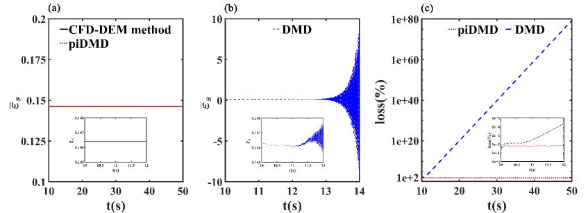
Figure 5: $(a)$ Simulation-domain-averaged solid phase volume fraction obtained from CFD-DEM simulation and piDMD-based long-term prediction. $(b)$ Simulation-domain-averaged solid phase volume fraction obtained from DMD-based long-term prediction. $(c)$ The $loss$ obtained from piDMD-based long-term prediction and DMD-based long-term prediction.

In addition to analyzing the accuracy of the instantaneous results of the piDMD-based long-term prediction, comparison between the time-averaged CFD-DEM results and the piDMD predicted results is shown in Fig.6. Fig.6 $(a)$ and $(b)$ compare the time-averaged flow field from $10\,$s to $50\,$s predicted by piDMD method and simulated by CFD-DEM method, where the CFD-DEM simulation is the time-averaged result of the instantaneous flow field with a time interval of $0.001\,$s in order to consistent with the piDMD-based prediction, although the time step for CFD-DEM simulation is $10^{-5}\,$s. It can be observed that the structure of the time-averaged flow field of piDMD-based long-term prediction is similar to that of the time-averaged flow field simulated by CFD-DEM method. Fig.6 $(c)$, $(d)$, and $(e)$ show the radial profiles of the time-averaged solid volume fraction at the axial heights of $48\,$mm, $96\,$mm, and $144\,$mm, respectively. Those figures reveal that the radial profiles of the time-averaged results of piDMD-based long-term prediction and CFD-DEM simulation are close at different heights. However, the results of piDMD-based long-term prediction are less smooth. Fig.6(f) displays the axial profiles of the time-averaged solid volume fraction obtained from CFD-DEM simulation and piDMD-based long-term prediction. Clearly, there are in a very good agreement.

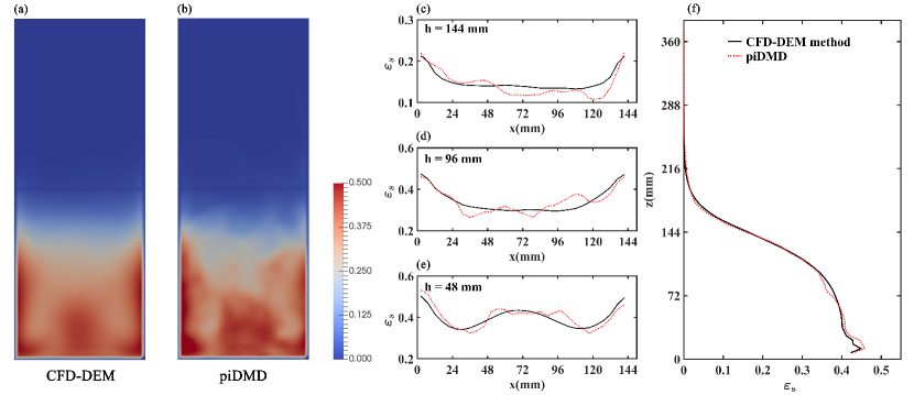
Figure 6: Comparison of time-averaged solid volume fractions obtained from CFD-DEM simulation and piDMD-based long-term prediction: $(a)$ and $(b)$ flow fields; the radial profiles at the bed heights of $(c)$ 144mm, $(d)$ 96mm, $(e)$ 48mm, and $(f)$ the axial profiles.

Overall, the results of piDMD-based long-term prediction have satisfactory time-averaged results compared to CFD-DEM simulation, but the accuracy of the instantaneous results needs to be improved. As can be seen from ${\mathbf{z}_{j+1,new}}=\mathbf{A}{\mathbf{z}_{j,new}}$, the error of each time step is accumulated to the next time step, which leads to the deviation of the instantaneous results, the development of physics-informed, streaming dynamic mode decomposition method (Hemati et al., 2014) might be a nice solution for further improving the prediction accuracy. A simple comparison of the piDMD method and other prediction methods is in order, the piDMD-based prediction is more efficient than the DeepVP proposed by Qin et al. (2023), which also predicted the voidage of bubbling fluidized bed, and took almost $525\,$h to build the DeepVP model at the first step, however, the whole process of the piDMD method predicts the physical time of $40\,$s flow field only takes $0.83\,$h. Furthermore, the ability of the piDMD method to predict solid phase volume fraction over long periods is significantly better than the convolutional neural network (CNN) trained by Bazai et al. (2021), whose model failed in generating correct contours of particle volume fraction in a fluidized bed compared to the result of CFD after $170$ time-steps (the time-step is $0.001\,$s).

5 Conclusion

A piDMD method is developed for predicting the solid volume fractions in a bubbling fluidized bed, where the physical law of mass conservation is integrated with the purely data-driven DMD method. On the basis of detailed comparison between the results of CFD-DEM simulation, piDMD-based prediction and DMD-based prediction, the following conclusions can be made: (i) The piDMD-based prediction ensures that the predicted sum of solid volume fractions will not change at any time, following the physical law of mass conservation in the bubbling fluidized bed; (ii) Both DMD and piDMD can predict the short-term behaviour of solid volume fraction reasonably well, but the piDMD method outperforms the DMD method in both qualitative and quantitative comparisons; (iii) The piDMD method is able to predict the flow field in the long time, and the instantaneous results are not accurate enough compared with CFD-DEM simulation, but the $loss$ values of the predicted field are stable, and the time-averaged results are satisfactory in terms of radial and axial profiles of solid volume fraction; (iv) The piDMD method is suitable for predicting the solid volume fraction distributions of bubbling fluidized beds very fast.

Appendix

Fig.7 compares the $loss$ values of the piDMD-based prediction of the same sampling data length ($5\,$s to $10\,$s) and different sampling frequencies ($1000\,$Hz, $500\,$Hz, $200\,$Hz, and $100\,$Hz). It is found that the loss values of the piDMD-based prediction with sampling frequencies of $1000\,$Hz and $500\,$Hz are the same, while the $loss$ values of the piDMD-based prediction with sampling frequencies of $200\,$Hz and $100\,$Hz are larger, indicating that the input data with smaller sampling frequencies do not contain enough characteristics of the bubbling fluidized bed.

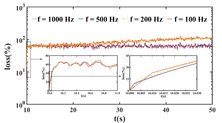
Figure 7: The $loss$ obtained from piDMD-based long-term prediction with its sampling frequency of $1000\,$Hz, $500\,$Hz, $200\,$Hz, and $100\,$Hz.

References

- Baddoo et al. (2023) Baddoo, P. J., Herrmann, B., McKeon, B. J., Nathan Kutz, J., Brunton, S. L., 2023. Physics-informed dynamic mode decomposition. Proceedings of the Royal Society A 479 (2271), 20220576.
- Baranidharan et al. (2022) Baranidharan, M., Kalel, D., Raja Singh, R., 2022. Potentials and challenges of digital twin: Toward industry 4.0. Smart Grids and Green Energy Systems, 75–90.
- Bazai et al. (2021) Bazai, H., Kargar, E., Mehrabi, M., 2021. Using an encoder-decoder convolutional neural network to predict the solid holdup patterns in a pseudo-2d fluidized bed. Chemical Engineering Science 246, 116886.
- Brunton et al. (2021) Brunton, S. L., Budišić, M., Kaiser, E., Kutz, J. N., 2021. Modern koopman theory for dynamical systems. arXiv preprint arXiv:2102.12086.
- Chen and Wang (2017) Chen, X., Wang, J., 2017. Dynamic multiscale method for gas-solid flow via spatiotemporal coupling of two-fluid model and discrete particle model. AIChE Journal 63 (9), 3681–3691.
- Chen and Wang (2018) Chen, X., Wang, J., 2018. Mesoscale-structure-based dynamic multiscale method for gas-solid flow. Chemical Engineering Science 192, 864–881.
- Cizmas et al. (2003) Cizmas, P., Palacios, A., O’Brien, T., Syamlal, M., 2003. Proper-orthogonal decomposition of spatio-temporal patterns in fluidized beds. Chemical engineering science 58 (19), 4417–4427.
- Curtis and Alford-Lago (2021) Curtis, C. W., Alford-Lago, D. J., 2021. Dynamic-mode decomposition and optimal prediction. Physical Review E 103 (1), 012201.
- Dabbagh et al. (2021) Dabbagh, F., Pirker, S., Schneiderbauer, S., 2021. A fast modeling of chemical reactions in industrial-scale olefin polymerization fluidized beds using recurrence CFD. AIChE Journal 67 (5), e17161.
- Fan (1996) Fan, L.-S., 1996. Summary paper on fluidization and transport phenomena. Powder Technology 88 (3), 245–253.
- Faridi et al. (2023) Faridi, I. K., Tsotsas, E., Heineken, W., Koegler, M., Kharaghani, A., 2023. Spatio-temporal prediction of temperature in fluidized bed biomass gasifier using dynamic recurrent neural network method. Applied Thermal Engineering 219, 119334.
- Ge et al. (2019a) Ge, W., Chang, Q., Li, C., Wang, J., 2019a. Multiscale structures in particle–fluid systems: Characterization, modeling, and simulation. Chemical Engineering Science 198, 198–223.
- Ge et al. (2019b) Ge, W., Guo, L., Liu, X., Meng, F., Xu, J., Huang, W. L., Li, J., 2019b. Mesoscience-based virtual process engineering. Computers & Chemical Engineering 126, 68–82.
- Ge et al. (2011) Ge, W., Wang, W., Yang, N., Li, J., Kwauk, M., Chen, F., Chen, J., Fang, X., Guo, L., He, X., et al., 2011. Meso-scale oriented simulation towards virtual process engineering (VPE)—the EMMS paradigm. Chemical Engineering Science 66 (19), 4426–4458.
- Ghadami and Epureanu (2022) Ghadami, A., Epureanu, B. I., 2022. Data-driven prediction in dynamical systems: recent developments. Philosophical Transactions of the Royal Society A 380 (2229), 20210213.
- Gidaspow (1994) Gidaspow, D., 1994. Multiphase flow and fluidization: continuum and kinetic theory descriptions. Academic press.
- Golshan et al. (2020) Golshan, S., Sotudeh-Gharebagh, R., Zarghami, R., Mostoufi, N., Blais, B., Kuipers, J., 2020. Review and implementation of CFD-DEM applied to chemical process systems. Chemical Engineering Science 221, 115646.
- Haghgoo et al. (2019) Haghgoo, M. R., Bergstrom, D. J., Spiteri, R. J., 2019. Analyzing dominant particle-flow structures inside a bubbling fluidized bed. International Journal of Heat and Fluid Flow 77, 232–241.
- Hajisharifi et al. (2023) Hajisharifi, A., Romanò, F., Girfoglio, M., Beccari, A., Bonanni, D., Rozza, G., 2023. A non-intrusive data-driven reduced order model for parametrized CFD-DEM numerical simulations. Journal of Computational Physics 491, 112355.
- Hemati et al. (2014) Hemati, M. S., Williams, M. O., Rowley, C. W., 2014. Dynamic mode decomposition for large and streaming datasets. Physics of Fluids 26, 111701.
- Higham et al. (2020) Higham, J., Shahnam, M., Vaidheeswaran, A., 2020. Using a proper orthogonal decomposition to elucidate features in granular flows. Granular Matter 22, 1–13.
- Holzmann (2016) Holzmann, T., 2016. Mathematics, numerics, derivations and OpenFOAM®. Loeben, Germany: Holzmann CFD.
- Jones et al. (2020) Jones, D., Snider, C., Nassehi, A., Yon, J., Hicks, B., 2020. Characterising the digital twin: A systematic literature review. CIRP Journal of Manufacturing Science and Technology 29, 36–52.
- Kieckhefen et al. (2020) Kieckhefen, P., Pietsch, S., Dosta, M., Heinrich, S., 2020. Possibilities and limits of computational fluid dynamics–discrete element method simulations in process engineering: A review of recent advancements and future trends. Annual Review of Chemical and Biomolecular Engineering 11, 397–422.
- Lan et al. (2020) Lan, B., Xu, J., Zhao, P., Zou, Z., Zhu, Q., Wang, J., 2020. Long-time coarse-grained CFD-DEM simulation of residence time distribution of polydisperse particles in a continuously operated multiple-chamber fluidized bed. Chemical Engineering Science 219, 115599.
- Li et al. (2023) Li, D., Zhao, B., Wang, J., 2023. Data-driven identification of coherent structures in gas–solid system using proper orthogonal decomposition and dynamic mode decomposition. Physics of Fluids 35 (1).
- Li et al. (2022a) Li, S., Duan, G., Sakai, M., 2022a. Development of a reduced-order model for large-scale Eulerian–Lagrangian simulations. Advanced Powder Technology 33 (8), 103632.
- Li et al. (2022b) Li, S., Duan, G., Sakai, M., 2022b. POD-based identification approach for powder mixing mechanism in Eulerian–Lagrangian simulations. Advanced Powder Technology 33 (1), 103364.
- Lichtenegger (2018) Lichtenegger, T., 2018. Local and global recurrences in dynamic gas-solid flows. International Journal of Multiphase Flow 106, 125–137.
- Lichtenegger and Pirker (2016) Lichtenegger, T., Pirker, S., 2016. Recurrence CFD–a novel approach to simulate multiphase flows with strongly separated time scales. Chemical Engineering Science 153, 394–410.
- Liu et al. (2020) Liu, X., Xu, J., Ge, W., Lu, B., Wang, W., 2020. Long-time simulation of catalytic mto reaction in a fluidized bed reactor with a coarse-grained discrete particle method–EMMS-DPM. Chemical Engineering Journal 389, 124135.
- Lu et al. (2016) Lu, L., Xu, J., Ge, W., Gao, G., Jiang, Y., Zhao, M., Liu, X., Li, J., 2016. Computer virtual experiment on fluidized beds using a coarse-grained discrete particle method–EMMS-DPM. Chemical Engineering Science 155, 314–337.
- Lu et al. (2014) Lu, L., Xu, J., Ge, W., Yue, Y., Liu, X., Li, J., 2014. EMMS-based discrete particle method (EMMS–DPM) for simulation of gas–solid flows. Chemical Engineering Science 120, 67–87.
- Lu et al. (2023) Lu, S., Lan, B., Xu, J., Zhao, B., Zou, Z., Wang, J., Li, H., Zhu, Q., 2023. Optimization of multiple-chamber fluidized beds using coarse-grained CFD-DEM simulations: Regulation of solids back-mixing. Powder Technology 428, 118886.
- Mezić (2013) Mezić, I., 2013. Analysis of fluid flows via spectral properties of the koopman operator. Annual review of fluid mechanics 45, 357–378.
- Qin et al. (2023) Qin, P., Xia, Z., Guo, L., 2023. A deep learning approach using temporal-spatial data of computational fluid dynamics for fast property prediction of gas-solid fluidized bed. Korean Journal of Chemical Engineering 40 (1), 57–66.
- Rowley et al. (2009) Rowley, C. W., Mezić, I., Bagheri, S., Schlatter, P., Henningson, D. S., 2009. Spectral analysis of nonlinear flows. Journal of Fluid Mechanics 641, 115–127.
- Schmid (2010) Schmid, P. J., 2010. Dynamic mode decomposition of numerical and experimental data. Journal of fluid mechanics 656, 5–28.
- Schmid (2022) Schmid, P. J., 2022. Dynamic mode decomposition and its variants. Annual Review of Fluid Mechanics 54, 225–254.
- Schönemann (1966) Schönemann, P., 1966. A generalized solution of the orthogonal procrustes problem. Psychometrika 31, 1–10.
- Stewart (1993) Stewart, G. W., 1993. On the early history of the singular value decomposition. SIAM review 35 (4), 551–566.
- Tao et al. (2018) Tao, F., Zhang, H., Liu, A., Nee, A. Y., 2018. Digital twin in industry: State-of-the-art. IEEE Transactions on Industrial Informatics 15 (4), 2405–2415.
- Tsuji et al. (1993) Tsuji, Y., Kawaguchi, T., Tanaka, T., 1993. Discrete particle simulation of two-dimensional fluidized bed. Powder Technology 77 (1), 79–87.
- Tu (2013) Tu, J. H., 2013. Dynamic mode decomposition: Theory and applications. Ph.D. thesis, Princeton University.
- van der Hoef et al. (2006) van der Hoef, M. A., Ye, M., van Sint Annaland, M., Andrews, A., Sundaresan, S., Kuipers, J., 2006. Multiscale modeling of gas-fluidized beds. Advances in Chemical Engineering 31, 65–149.
- Wang (2020) Wang, J., 2020. Continuum theory for dense gas-solid flow: A state-of-the-art review. Chemical Engineering Science 215, 115428.
- Wen et al. (2023) Wen, K., Guo, L., Xia, Z., Chen, J., 2023. A rapid simulation method of gas-solid flow by coupling CFD and deep learning. CIESC Journal, DOI:10.11949/0438–1157.20230711.
- Xu et al. (2019) Xu, J., Liu, X., Hu, S., Ge, W., 2019. Virtual process engineering on a 3D circulating fluidized bed with multi-scale parallel computation. Journal of Advanced Manufacturing and Processing 1, 10014.
- Xu et al. (2011) Xu, J., Qi, H., Fang, X., Lu, L., Ge, W., Wang, X., Xu, M., Chen, F., He, X., Li, J., 2011. Quasi-real-time simulation of rotating drum using discrete element method with parallel GPU computing. Particuology 9 (4), 446–450.
- Xu et al. (2022) Xu, J., Zhao, P., Zhang, Y., Wang, J., Ge, W., 2022. Discrete particle method for engineering simulation: Reproducing mesoscale structures in multiphase systems. Resources Chemicals and Materials 1, 69–79.
- Yu et al. (2021) Yu, J., Lu, L., Gao, X., Xu, Y., Shahnam, M., Rogers, W. A., 2021. Coupling reduced-order modeling and coarse-grained CFD-DEM to accelerate coal gasifier simulation and optimization. AIChE Journal 67 (1), e17030.
- Yu et al. (2015) Yu, M., Miller, D. C., Biegler, L. T., 2015. Dynamic reduced order models for simulating bubbling fluidized bed adsorbers. Industrial & Engineering Chemistry Research 54 (27), 6959–6974.
- Yuan et al. (2005) Yuan, T., Cizmas, P., O’Brien, T., 2005. A reduced-order model for a bubbling fluidized bed based on proper orthogonal decomposition. Computers & chemical engineering 30 (2), 243–259.
- Zhang et al. (2020a) Zhang, Y., Jia, Y., Xu, J., Wang, J., Duan, C., Ge, W., Zhao, Y., 2020a. CFD intensification of coal beneficiation process in gas-solid fluidized beds. Chemical Engineering and Processing-Process Intensification 148, 107825.
- Zhang et al. (2020b) Zhang, Y., Jiang, M., Chen, X., Yu, Y., Zhou, Q., 2020b. Modeling of the filtered drag force in gas–solid flows via a deep learning approach. Chemical Engineering Science 225, 115835.
- Zhang et al. (2023) Zhang, Y., Xu, J., Chang, Q., Zhao, P., Wang, J., Ge, W., 2023. Numerical simulation of fluidization: Driven by challenges. Powder Technology 414, 118092.
- Zhang et al. (2019) Zhang, Y., Zhao, Y., Gao, Z., Duan, C., Xu, J., Lu, L., Wang, J., Ge, W., 2019. Experimental and eulerian-lagrangian-lagrangian study of binary gas-solid flow containing particles of significantly different sizes. Renewable Energy 136, 193–201.
- Zhang et al. (2017) Zhang, Y., Zhao, Y., Lu, L., Ge, W., Wang, J., Duan, C., 2017. Assessment of polydisperse drag models for the size segregation in a bubbling fluidized bed using discrete particle method. Chemical Engineering Science 160, 106–112.
- Zhao et al. (2022a) Zhao, P., Xu, J., Chang, Q., Ge, W., Wang, J., 2022a. Euler-lagrange simulation of dense gas-solid flow with local grid refinement. Powder Technology 399, 117199.
- Zhao et al. (2020a) Zhao, P., Xu, J., Ge, W., Wang, J., 2020a. A CFD-DEM-IBM method for cartesian grid simulation of gas-solid flow in complex geometries. Chemical Engineering Journal 389, 124343.
- Zhao et al. (2020b) Zhao, P., Xu, J., Liu, X., Ge, W., Wang, J., 2020b. A computational fluid dynamics-discrete element-immersed boundary method for cartesian grid simulation of heat transfer in compressible gas–solid flow with complex geometries. Physics of Fluids 32 (10), 103306.
- Zhao et al. (2022b) Zhao, P., Xu, J., Zhao, B., Li, D., Wang, J., 2022b. Cartesian grid simulation of reacting gas-solid flow using CFD-DEM-IBM method. Powder Technology 407, 117651.
- Zhong et al. (2020) Zhong, H., Xiong, Q., Yin, L., Zhang, J., Zhu, Y., Liang, S., Niu, B., Zhang, X., 2020. CFD-based reduced-order modeling of fluidized-bed biomass fast pyrolysis using artificial neural network. Renewable Energy 152, 613–626.