A Markovian approach to the Prandtl-Tomlinson frictional model

Abstract

We consider the Prandtl-Tomlinson model in the case of a constant driving force and in the presence of thermal fluctuations. We show that the system dynamics is well reproduced by a simplified description obtained through a Markov process, even in the case of potentials with several minima. After estimating the chain parameters by numerical simulation, we compute the average velocity and friction at varying driving force and temperature. Then we take advantage of this approach for calculating the entropy produced by the system and, in the case of a single minimum potential, to derive its explicit relation with the external force and the mobility at low temperatures. We observe that the coefficient relating the entropy production to the force is not a monotonic function of the temperature.

1 Introduction

Among the simplified models for solid-on-solid friction, the now so called Prandtl-Tomlinson (PT) model has recently seen renewed interest because of its suitability to the description of atomic force microscopy [1, 2]. As already pointed out in [3] this model mainly originates from a work of L. Prandtl [4] and has very limited relevance with the model for friction devised by G. Tomlinson [5] (a summary of its history and different contributions can be found in several reviews, e.g. [3] and [6]). In its present acceptation the PT model describes the dissipative motion of a particle on a periodic substrate, and in its more general formulation it is defined by the Langevin equation

$$m\ddot{x}=f(x)-\partial_{x}U(x)-\gamma\dot{x}+\sqrt{2\gamma k_{B}T}\xi(t),$$ (1)

being $m$ is the mass of the probe particle, $f(x)$ an external force acting on the probe, and $\gamma$ a viscous coefficient; $U$ is a periodic function, $U(x+L)=U(x)$, representing the substrate characterized from some crystalline order. Here the effect of temperature, $T$, is given by the last term which derives its form from the Einstein’s dissipation-fluctuation relation, linking the noise amplitude to the viscosity and the Boltzmann constant $k_{B}$. Depending on the choice of $f(x)$, different implementations of the model are possible [3]. While the case of a probe driven by a compliant harmonic force with constant drift, $f(x)=-k(vt-x),$ has been widely investigated [7, 8, 9, 10, 11], here we focus on the case of a constant driving force, $f(x)=F$, which can be relevant to the description of macroscopic interfaces and has been much less studied. Recent work on this case has focused mainly on the lowering of the critical energy barriers with increasing the driving force [12, 13].

In this paper we describe the dynamics of the PT model as a Markov chain where the relevant states are the potential minima. By investigating the stationary average speed and friction we find that such process can effectively well describe the system in a wide range of $F$ and $T$, allowing to simplify the calculation of quantities of interest, such as the mobility and the entropy production rate. For illustration we shall consider both the case of a substrate potential displaying a single minimum per period and that in which several periodic minima are present.

In Section 2 we briefly discuss the general reasons to adopt a description in terms of Markov chain, as well as the basic mathematical aspects and the numerical results. Section 3 is devoted to the investigation of friction and velocity, including an evaluation of the mobility, whereas Sec. 4 concerns the entropy production. Section 5 shortly investigates an instance of a substrate displaying $m$ minima and reports the behavior of mobility and entropy production for the specific case of $m=4$. Section 6 summarizes the main results.

2 Markov description: conceptual and numerical determination

Often in experimental or numerical measurements, the state of a physical system cannot be determined with arbitrary accuracy. This implies the possibility (necessity) to introduce probabilistic methods using suitable stochastic description. In particular, a description in terms of Markov chains, which is quite natural and (relatively) simple, had been used with success in many different contexts [14]. Such an approach can be used just from the knowledge of experimental data and even in absence of a good model.

In a Markov chain [15], time is discretized into intervals $\tau$ and the process is described by a numerable set of states $\{s\}$, with the assumption that the conditional probability that the system at time $t_{n}$ is in the state $s_{\alpha}$, knowing the past, i.e. the states at times $t_{n-1}$, $t_{n-2}$, and so on, depends only by the state $s_{\beta}$ assumed at the previous time $t_{n-1}$:

$$P(t_{n},s=s_{\alpha}\mid t_{n-1},s=s_{\beta};t_{n-2},s=s_{\gamma};\dots)=$$ (2)

$$=P(t_{n},s=s_{\alpha}\mid t=t_{n-1},s=s_{\beta}).$$ (3)

Then if the process is homogeneous in time, it is completely characterized by the conditional probabilities $\hat{T}_{\alpha,\beta}=P(t_{n},s=s_{\alpha}\mid t_{n-1,}s=s_{\beta})$,. The elements of such transition matrix cannot be completely arbitrary: $0\leq\hat{T}_{\alpha,\beta}\leq 1$ with $\sum_{\alpha}\hat{T}_{\alpha,\beta}=1$ because of the normalization.

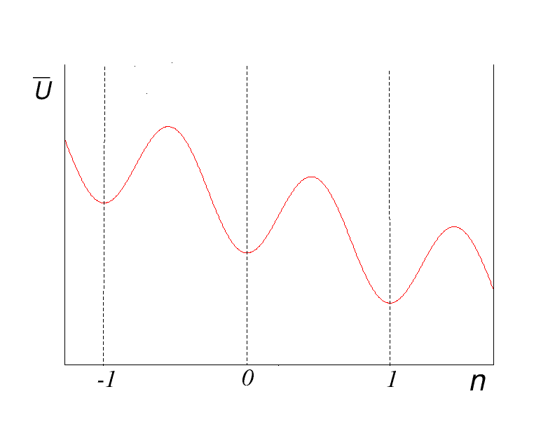
Figure 1: Schematic of the, one minimum, potential landscape for the probe particle.

To describe effectively the stationary system dynamics, at each time step we associate the particle coordinate to the closest minimum of $\bar{U}(x)=U(x)-Fx$. For sake of simplicity let us consider the simplest case in Fig. 1 where 3 minima are shown. For time intervals $\tau$ small enough, the probability for the particle to perform a jump with $\mid\Delta n\mid>1$ is negligible. After a sampling time $\tau$, we again associate the coordinate of the particle to the nearest minimum of $\bar{U}(x)$. Then, we set the state of the Markov chain $s=1,-1,0$ depending on whether the particle has jumped to the next, previous or current minimum respectively. It should be noted that the sampling time $\tau$ may differ from the integration time step. However, the results are weakly dependent on $\tau$ (at least for values of $\tau$ neither too large nor too small). The transition matrix can be empirically estimated by the ratio between the number of transitions $N_{ij}$ from $i$ to $j$, with $i,j=0,\pm 1$, and the number of times $N_{i}$ that $i$ occurred :

$$\hat{T}_{i,j}=\frac{N_{ij}}{N_{i}}\quad\text{with}\quad i,j=-1,0,1$$ (4)

Being the system periodic, the transition probabilities $\hat{T}_{i,j}$ are independent from the initial state $i$. By writing them as:

$$\hat{T}_{i,1}=p_{+}\quad\hat{T}_{i,0}=p_{0}\quad\hat{T}_{i,-1}=p_{-}$$ (5)

the stochastic matrix reduces to:

$$\hat{T}=\begin{pmatrix}p_{-}&p_{0}&p_{+}\\ p_{-}&p_{0}&p_{+}\\ p_{-}&p_{0}&p_{+}\end{pmatrix}.$$ (6)

The stationary probability distribution satisfies

$$P^{\left\{s\right\}}=P^{\left\{s\right\}}\hat{T},$$

and corresponds therefore to the row eigenvector associated with the maximum eigenvalue of $\hat{T}$, $\lambda=1$:

$$P^{\left\{s\right\}}=\begin{pmatrix}p_{-},\quad p_{0},\quad p_{+}\end{pmatrix},$$ (7)

whose components can be empirical estimated as

$$P^{\left\{s\right\}}_{i}=\frac{N_{i}}{\sum_{j}{N_{j}}}.$$ (8)

Now that we have introduced the general concepts, let’s see how this works in practice.

Consider the PT model, eq. (1) with constant external force $F$ and a periodic potential $U(x)$:

$$U(x)=\frac{U_{0}L}{2\pi}\sin\biggl{(}\frac{2\pi}{L}x\biggr{)}.$$ (9)

Notice that Eq. (1) can be made adimensional by introducing the natural units of mass $m$, time $m/\gamma$ and length $L$, turning into

$$\ddot{x}=F-\partial_{x}U(x)-\dot{x}+\sqrt{2T}\xi(t),$$ (10)

(where all quantities, $x$, $F$, $U$ are now to be intended as expressed in the natural units), showing that therefore there are only two free parameters, e.g. $F/U_{0}$ and $T/U_{0}$. For the sake of clarity in the following we shall maintain the explicit dependence on $L$.

To evaluate the transition matrix $\hat{T}$, we resort to an integration algorithm from [16]. At each time step the position $x(t)$ of the particle is recorded, and after a sampling time step $\tau$ the closest minimum point of the potential is determined. The state $s=1,-1,0$ is associated to the particle depending if the particle is in the basin of attraction of the next, the same, or the previous potential minimum (notice that the state describes the transition and not to the visited minimum).

For all the numerical computations the maximum potential amplitude is set to $U_{0}=0.1$ and the sampling time $\tau=0.1$, with maximum computational time $t_{max}=10^{5}$ (the dependence of the results on the value of $\tau$ is very weak). Empirical averages are estimated over $N=10^{3}$ different realizations of the noise with identical initial conditions for particle position and velocity. As an example, for $F=0.08$ and $T=0.01$ we obtain:

$$\hat{T}=\begin{pmatrix}0.00009&0.99554&0.00437\\ 0.00009&0.99543&0.00448\\ 0.00007&0.99529&0.00464\end{pmatrix},$$ (11)

with little fluctuations in the columns as consequence of numerical round-off errors in the numerical integration process.

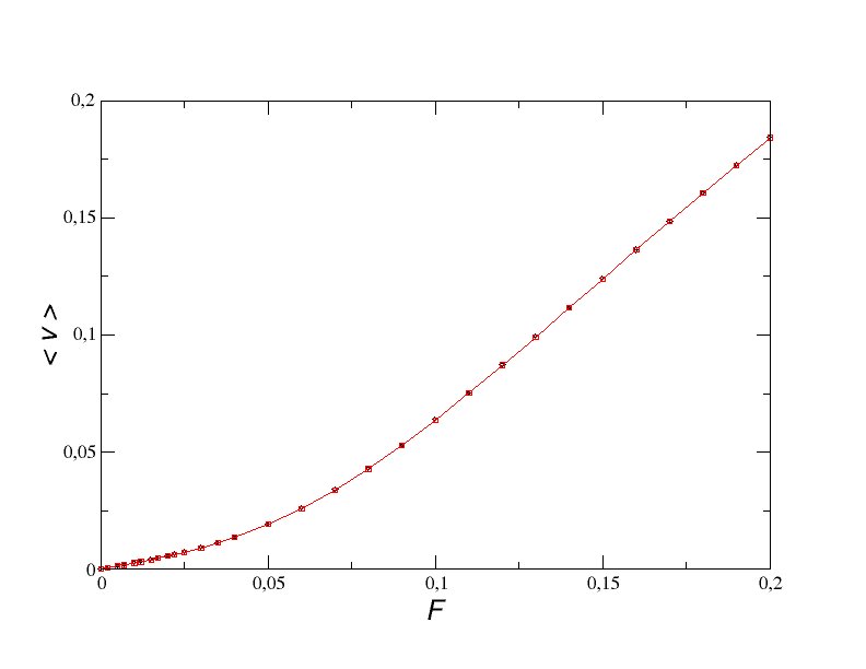
Figure 2: Comparison of the average particle speed obtained from direct motion integration (circles, black on-line) and from Markov chain description (squares, red on-line) and ) for a substrate potential with a single minimum per period, at $T=0.01$

3 Markov average velocity and friction

As a test for the goodness of this description we compare the average speed $\langle v\rangle$ obtained from the Markovian approximation

$$\langle{v}\rangle=\frac{L}{\tau}(p_{+}v_{1}+p_{0}v_{0}+p_{-}v_{-1})=\frac{L}{\tau}(p_{+}-p_{-})$$ (12)

with that obtained by direct integration of the motion equation, averaging on both time and different realizations of the process:

$$\bar{v}=\frac{1}{t_{max}}\sum_{i=0}^{t_{max}}\langle v(t_{i})\rangle,$$ (13)

where $\langle\rangle$ stays here for the average over the different realizations. Figure 2 shows that there is a very good agreement between the values obtained using the two methods for different values of the force $F$ at the temperature $T=0.01$ (with relative errors always smaller than $10^{-3}$).

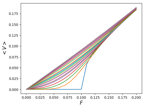
Figure 3: Average velocity as function of the external driving force in a one minimum potential for different $T$. The lowest curve (red on-line) corresponds to $T=0$. The other curves, from bottom to top, represent increasing temperatures in the range [0.003,0.05] corresponding to those of the points in Fig. 4.

We then adopt the Markovian parametrization to investigate the behavior of $\langle v\rangle$ with $F$ at different temperatures. Results are shown in Fig. 3 As expected the curve for $T=0$ displays no motion as far as $F<U_{0}$ and is singular in $F=U_{0}$. For $T>0$ curves are smooth and display increasing values of the average velocity with $T$. For increasing temperature the average speed becomes essentially proportional to $F$ since, as it will be shown below, friction tends to vanish. At the same time thermal fluctuations become negligible for increasing $F$.

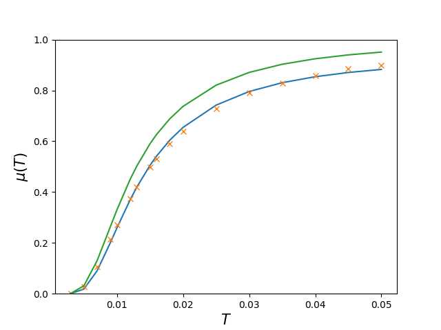
Figure 4: Mobility $\mu$ as function of the bath temperature $T$ for a potential with one minimum as resulting from the Markov chain (crosses). The upper curve (green on-line) is obtained from the approximated expression derived in [17] in the high friction limit. The other curve (orange on-line) is best-fit to the points by a generalization of the same expression (see text).

For $F\ll U_{0}$, on very general bases one expects for any $T$:

$$\langle v\rangle=\mu\cdot F,$$ (14)

where $\mu=\mu(T)$ is the particle mobility. Its values can be obtained from the data of Fig. 3 by considering the values of $\langle v\rangle$ at small $F$. The behavior resulting from considering values below $F=0.025\ll U_{0}$ is shown by the points in Fig. 4. In the figure it is also reported the behavior resulting from the approximated derived in [17] in the high friction limit (upper curve, green on-line)

$$\mu=\frac{I_{0}^{-2}(U_{0}/T)}{\gamma},$$ (15)

where $I_{0}$ is the modified Bessel function. The lower curve is a best fit to the points obtained by inserting in an arbitrary proportionality factor between the two sides of the above equation and by letting it and $L$ to change suitably.

Taking thermal averages in eq. (10), in the steady state one has $\langle\ddot{x}\rangle=0$ and $\langle\xi(t)\rangle=0$, and the average speed is:

$$\langle v\rangle=\langle\dot{x}\rangle=\frac{F-\langle\partial_{x}U(x)\rangle}{\gamma}.$$ (16)

Averages are performed on the probability distribution, that in turn depends on the force $F$, that can be determined by the associate Fokker-Planck equation. On the other hand in a deterministic system subjected to an average dynamic friction force $F_{d}$ and a viscous coefficient $\gamma$, the stationary average speed of the particle is:

$$\langle v\rangle=\frac{F-F_{d}}{\gamma}.$$ (17)

Thus one identifies the average value of the derivative of the interaction potential in (16) with the average dynamic friction, which in turn depends on $F$:

$$F_{d}(F)=\langle\partial_{x}U(x)\rangle.$$ (18)

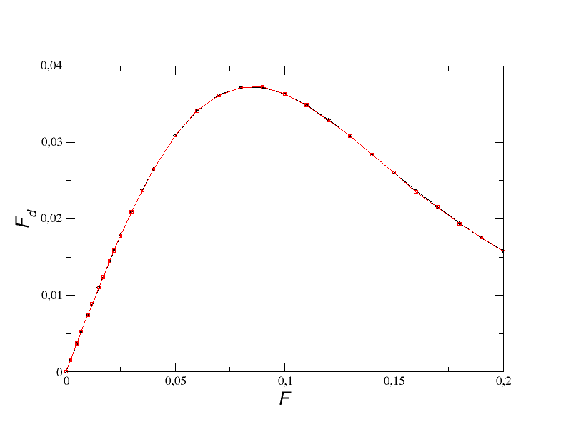
Figure 5: Comparison of the average friction force acting on the particle, subjected to a single minimum periodic potential, as obtained from direct motion integration (circles, black on-line) and from the Markov chain, as difference between the average velocity and the driving force (squares, red on-line). $T=0.01$.

As a further test for the Markovian description we then compare the effective dynamic friction, eq. (18), resulting from the Markov chain via eq. (16) with that obtained by the numerical integration of motion. The two are shown in Fig. 5 displaying even in this case a very good agreement and relative differences smaller than $10^{-3}$. As expected $F_{d}$ displays a maximum in correspondence of the value of $F=U_{0}$, and decreases for larger values, so that $\langle v\rangle\to F/\gamma$.

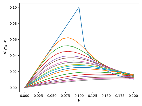
Figure 6: Average dynamic friction, in a single minimum potential, as function of the external driving force for different $T$. The upmost curve (red on-line) corresponds to $T=0$. The other curves represent temperatures in the range [0.003,0.05], decreasing from top to bottom, and correspond to the temperatures of the points in Fig. 4.

Figure 6 displays $F_{d}$, computed via the stochastic matrix, as function of $F$ for different temperatures ranging from $T=0$ to $T=0.05$. For $T=0$, corresponding to the uppermost curve, the average friction equals the driving force, with a discontinuous derivative, indicating static equilibrium for any value $F\leq U_{0}$, and corresponding therefore to a static friction. For $T\neq 0$ the particle can jump from a local potential well to another one for any value of $F$ and $U_{0}$. If $F=0$ the probability of moving forward to the next minimum is equal to that of moving backward, and the average speed is zero. When $F\neq 0$, its direction is favored and the average speed is different from zero, implying $\langle\partial_{x}U(x)\rangle<F$ even if $F\ll U_{0}$. As expected, the general effect of thermal fluctuation is to decrease friction, whose values tend to become similar for $F\gg U_{0}$. It is however interesting to notice that the minimum friction at large $F$ is obtained for $T=0$ .

4 Entropy production

One advantage of the description in terms of a Markov chain is that it allows to define and compute in a simple way the entropy production of the process along system’s trajectories. The only required condition is that if $\hat{T}_{i,j}>0$, then also $\hat{T}_{j,i}>0$. Within this frame the probability of observing a trajectory of length $n$ starting from the state $s_{0}$ and ending in $s_{n}$, $\{s_{0};s_{1};\dots;s_{n}\}$, can be expressed as

$$\mathit{P}(s_{0};\dots;s_{n})=\hat{T}_{n,n-1},\dots\hat{T}_{2,1}\hat{T}_{1,0}\pi_{0}$$ (19)

and similarly, the probability of the reverse trajectory is:

$$\mathit{P}(s_{n};\dots;s_{0})=\hat{T}_{0,1}\dots\hat{T}_{n-2,n-1}\hat{T}_{n-1,n}\pi_{n}$$ (20)

where $\pi_{0}$ and $\pi_{n}$ are the invariant probabilities of $s_{0}$ and $s_{n}$. The entropy production along the path can then be computed as [18, 19]:

$$\begin{split}\Sigma_{n}&=\ln{\biggl{(}\frac{\mathit{P}(s_{0};\dots;s_{n})}{\mathit{P}(s_{0};\dots;s_{n})}\biggr{)}}-\ln{\biggl{(}\frac{\pi_{0}}{\pi_{n}}\biggr{)}}=\\ &=\sum_{k=1}^{n}\ln{\biggl{(}\frac{\hat{T}_{\alpha_{k},\alpha_{k-1}}}{\hat{T}_{\alpha_{k-1},\alpha_{k}}}\biggr{)}}\end{split}.$$ (21)

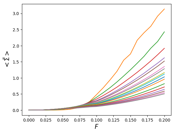
Figure 7: Average rate of entropy production $<\tilde{\Sigma}>$, for the case of periodic potential with a single minimum, as function of the driving force $F$ at temperatures corresponding to those of the points of Fig. 8, with increasing values when going from top to bottom.

To calculate it we observe that the position of the particle at the time $t_{n}$ is related to the states of the Markov chain through:

$$x_{n}=x_{n-1}+\delta_{n}$$ (22)

where $\delta_{n}$ assumes the values: $-L,0,L$ with probabilities $p_{+}$, $p_{-}$ e $p_{0}$, respectively. If at time $n=0$ the position of the particle $x_{0}$ is in the state $\alpha_{0}$, the probability of observing a given trajectory $\{x_{0};x_{1};\dots;x_{n}\}$. depends therefore exclusively on the probability of the initial state and on number of times, $n_{+}$, $n_{-}$ and $n_{0}$, that $\delta_{k}$ takes the value $L$, $-L$ and $0$:

$$\mathit{P}(x_{0};\dots;x_{n})=\pi_{0}p_{+}^{n_{+}}p_{-}^{n_{-}}p_{0}^{n_{0}}$$ (23)

The probability for the inverse trajectory is obtained by exchanging the number of forward and backward transitions $n_{+}$ and $n_{-}$:

$$\mathit{P}(x_{n};\dots;x_{0})=\pi_{n}p_{+}^{n_{-}}p_{-}^{n_{+}}p_{0}^{n_{0}},$$ (24)

and the entropy production results in

$$\Sigma=\ln{\biggl{(}\frac{p_{+}^{n_{+}}p_{-}^{n_{-}}p_{0}^{n_{0}}}{p_{+}^{n_{-}}p_{-}^{n_{+}}p_{0}^{n_{0}}}\biggr{)}}=(n_{+}-n_{-})\ln{\biggl{(}\frac{p_{+}}{p_{-}}\biggr{)}}.$$ (25)

In the limit $n\gg 1$, the number of forward jumps $n_{+}$ and backward jumps $n_{-}$ tends to their expected values, $np_{+}$ and $np_{-}$, and the entropy production rate $<\tilde{\Sigma}>=\frac{\Sigma}{n\tau}$ assumes the average value

$$\langle\tilde{\Sigma}\rangle=\frac{1}{\tau}(p_{+}-p_{-})\ln{\biggl{(}\frac{p_{+}}{p_{-}}\biggr{)}}.$$ (26)

The resulting behavior as function of $F$ is shown in Fig. (7) for various temperatures between $T=0.003$ (the upper curve, red on-line) and $T=0.05$ (the lower curve, dark pink on-line). As thermal fluctuations become less relevant, the entropy production increases because of the decrease of $p_{-}$.The behavior for $F\ll U_{0}$ can be understood by observing that in this case probabilities $p_{+}$ and $p_{-}$ do not differ too much one each other and can be written as:

$$p_{+}=p+\epsilon_{1}$$ (27)

$$p_{-}=p-\epsilon_{2}$$ (28)

with $\epsilon_{1},\epsilon_{2}\ll 1$. By expanding the logarithm in (26), and considering that $\langle v\rangle=\frac{L}{\tau}(\epsilon_{1}+\epsilon_{2})$, one then obtains:

$$\langle\tilde{\Sigma}\rangle\simeq\frac{(\epsilon_{1}+\epsilon_{2})^{2}}{p\tau}=\frac{<v>^{2}\tau}{pL^{2}},$$ (29)

or

$$\langle\tilde{\Sigma}\rangle\simeq c(T)F^{2},$$ (30)

with

$$c(T)=\frac{\tau}{L^{2}p}\,\mu^{2}(T).$$ (31)

The behavior of $c(T)$ is shown in Fig.8 and displays a relative maximum. The continuous (orange) curve is obtained by a fit with the expression eq. (31).

Finally let us observe that the entropy production is proportional to the current:

$$J_{n}=\sum_{k=1}^{n}{\delta_{k}},$$ (32)

an interesting quantity for systems far from the equilibrium.

Let us stress that it is possible to adopt a Markov description in the analysis of experimental data even in absence of a detailed model. In fact, it is enough to identify the relevant variables which describe the systems. Furthermore, it allows to define and compute in a relatively simple way the entropy production of the system avoiding the complications that arise in the continuous description due to the non-invertibility of the noise matrix.

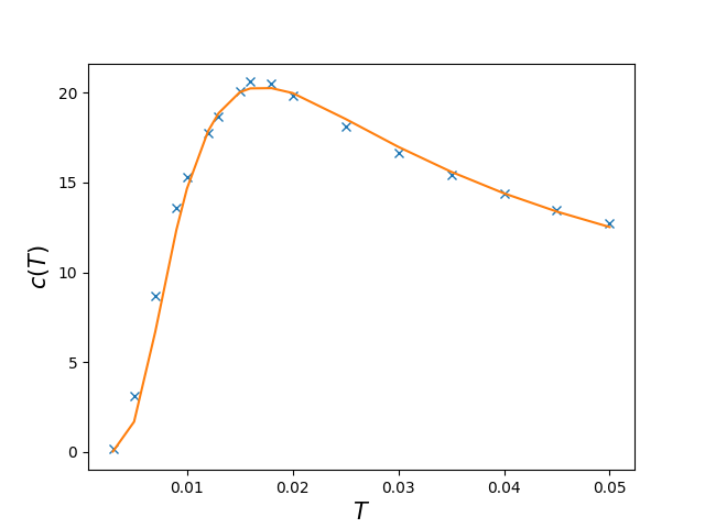
Figure 8: Proportionality constant $c(T)$ between the entropy production rate and $F^{2}$ at low $F$ for one-minimum potential.

5 Corrugated potential

The above analyses can be easily repeated also for the case of a potential displaying several minima within each period. One way to obtain such potential is to add to $U(x)$ another periodic term with amplitude $\Delta_{0}$, and period, $l$:

$$U(x)=\frac{U_{0}L}{2\pi}\sin\biggl{(}\frac{2\pi}{L}x\biggr{)}+\frac{\Delta_{0}l}{2\pi}\sin\biggl{(}\frac{2\pi}{l}x\biggr{)},$$ (33)

with $L=ml$. The number of relative minima depends on the choice of $\Delta_{0}$ and ranges between $0$ and $m$ . As an instance, we choose $l=L/4$, and $\Delta_{0}=3U_{0}$, so $U(x)$ displays four minima within one period $L$ and there are four equilibrium points determined by the condition

$$F-U_{0}\cos\biggl{(}\frac{2\pi}{L}x\biggr{)}-\Delta_{0}\cos\biggl{(}\frac{8\pi}{L}x\biggr{)}=0.$$ (34)

In this case, the states of the Markov chain $s=0,1,2,3$ correspond to the basins of attraction of the relative minima of the potential (see Fig. 9).

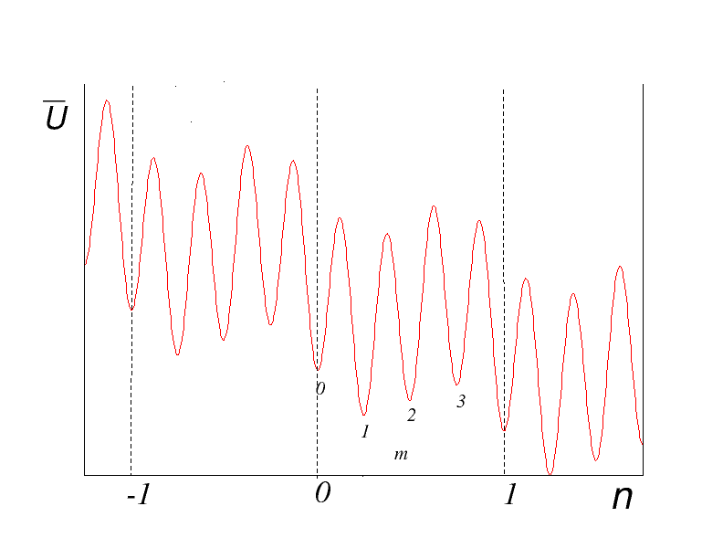
Figure 9: Schematic of the corrugated potential landscape for the probe particle. The small numbers indicate the states $s$ of the Markov chain.

Although in this case also transitions between different, not necessarily neighboring, secondary minima are allowed, the observed dependence of the average friction $F_{d}$ and speed on the external force $F$ and temperature $T$ results qualitatively very similar to the case of a single minimum, as shown in Fig. 10. The figure also shows (upper curve, green on-line) the behavior as resulting from the high friction limit expression [17]:

$$\mu=\left(\frac{2\pi}{\gamma\int_{0}^{2\pi}e^{U/T}dx}\right)^{2}.$$ (35)

The lower curve (orange on-line) is obtained by fitting of the points with the same expression but adjusting $L$ and an arbitrary prefactor.

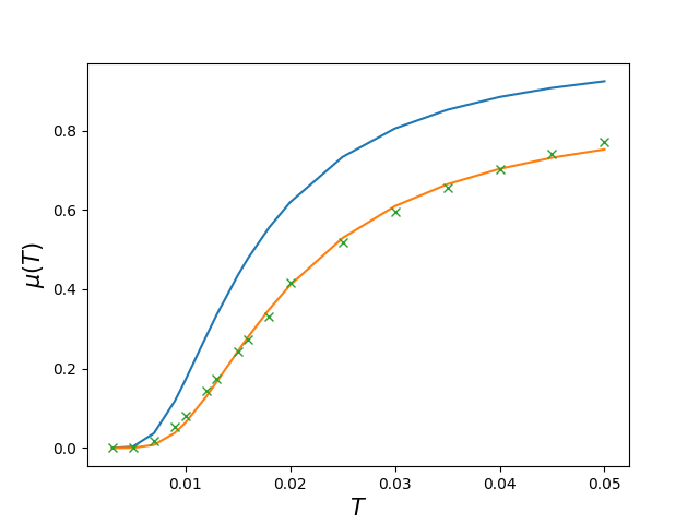
Figure 10: Mobility $\mu$ as function of the bath temperature $T$ for a potential with four minima (crosses). The upper curve (blue on-line) is obtained from the approximate expression derived in [17]. The lower curve (orange on-line) is given by a best-fit of a generalization of this expression (see text) to the points.

More interesting appears the behavior of the entropy. In this case, simple manipulations lead to the following expression for the average rate of entropy production over a trajectory of length $t=n\tau$:

$$\langle\tilde{\Sigma}\rangle=\frac{1}{n\tau}\sum_{i=0}^{3}{(\pi_{i}\hat{T}_{i,i+1}-\pi_{i+1}\hat{T}_{i+1,i})\log{\biggl{(}\frac{\hat{T}_{i,i+1}}{\hat{T}_{i+1,i}}\biggr{)}}}$$ (36)

where $\pi_{i}$ is the stationary probability of observing the particle close to the $i$th secondary minimum ($i=0,1,2,3$).

The resulting dependence on $F$ at different $T$ is shown in Fig. 11.

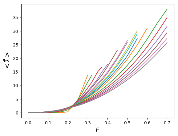
Figure 11: Average entropy production rate $<\tilde{\Sigma}>$ as function of the driving $F$ for a four-minima potential. The different curves correspond to the temperatures of the points in Fig. 12, with increasing values from the shortest to the longest. For large $F$ inverse trajectories are forbidden at low $T$.

The first thing that can be noted is that the entropy production cannot be calculated for each value of the force $F$ since at low temperature thermal fluctuations are not enough strong to allow the particle to jump backward for large $F$. On the other hand, in analogy to the case of a single minimum, $\langle\tilde{\Sigma}\rangle$ is proportional to $F^{2}$ for small $F$. The resulting proportionality coefficient $c(T)$ is shown in Fig. (12). At variance with the one-minimum potential the maximum is much less pronounced.

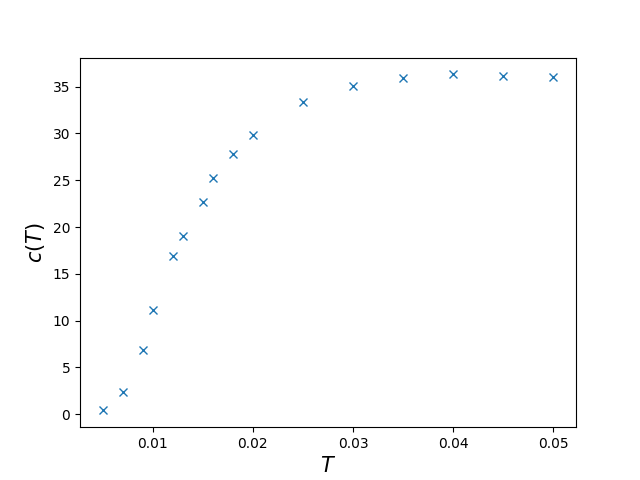
Figure 12: Proportionality constant $c(T)$ between the entropy production rate and $F^{2}$ at low $F$ for a four-minima potential.

6 Summary

In this paper we have investigated the stationary state of the inertial Prandtl-Tomlinson model in a thermal bath describing it by a suitable Markov chain. The description in terms of a Markov chain is rather flexible and can be used even in presence of lack of an accurate model: it suffices to know the proper variables.

We have considered in particular the less investigated instance of a constant driving force, considering the periodic potential in both the case of a single minimum and of many minima per period. At variance with other approaches [9, 20, 21, 22, 10, 13] we have not estimated the transition rates from Arrhenius or Kramers expressions but by direct numerical simulations of the system’s dynamics, as described by the corresponding Langevin equation. Under the assumption that at each sampling time step the probe particle could jump at most the distance of one period of the potential, we have computed friction and velocity from the Markov chain for a wide range temperatures $T$ and driving forces $F$, finding excellent agreement with the values obtained by direct simulations.

With this approach we have then been able to investigate also the behavior of the entropy production. To our knowledge this has been studied only recently by Torche and coworkers [23] for the case of a compliant driving, starting from a master equation with Arrhenius transition rates. We have considered the periodic potential in both the case of one single minimum and of many minima per period. We have derived an explicit expression for the case of a single minimum at low temperature, finding that in this limit the entropy production is proportional to the square of the external force, and that the proportionality coefficient displays a non monotonic behavior as function of the temperature.

References

- [1] Y. Dong, A. Vadakkepatt, A. Martini, Analytical models for atomic friction, Tribology Letters 44 (3) (2011) 367–386. doi:10.1007/s11249-011-9850-2.
- [2] A. Vanossi, N. Manini, M. Urbakh, S. Zapperi, E. Tosatti, Colloquium: Modeling friction: From nanoscale to mesoscale, Reviews of Modern Physics 85 (2) (2013) 529–552. arXiv:1112.3234, doi:10.1103/RevModPhys.85.529.
- [3] V. L. Popov, J. A. Gray, Prandtl-Tomlinson model: History and applications in friction, plasticity, and nanotechnologies, ZAMM Zeitschrift fur Angewandte Mathematik und Mechanik 92 (9) (2012) 683–708. doi:10.1002/zamm.201200097.
-
[4]
L. Prandtl,
Ein
Gedankenmodell zur kinetischen Theorie der festen Körper, Zeitschrift fr
Angewandte 8 (1928) 85, English translation: A Conceptual Model to the
Kinetic Theory of Solid Bodies, Translated from German original by V. L.
Popov and J. Gray, Berlin University of Technology.
URL https://www.reibungsphysik.tu-berlin.de/fileadmin/fg204/Publikationen/Prandtl_1928_English.pdf - [5] G. Tomlinson, A molecular theory of friction, Philos. Mag. 7 (1929) 905–939.
- [6] H. Spikes, W. Tysoe, On the Commonality between Theoretical Models for Fluid and Solid Friction, Wear and Tribochemistry, Tribology Letters 59 (1) (2015) 1–14. doi:10.1007/s11249-015-0544-z.
- [7] C. Fusco, A. Fasolino, Velocity dependence of atomic-scale friction: A comparative study of the one- and two-dimensional Tomlinson model, Physical Review B - Condensed Matter and Materials Physics 71 (4) (2005) 1–9. arXiv:0502496, doi:10.1103/PhysRevB.71.045413.
- [8] J. Nakamura, S. Wakunami, A. Natori, Double-slip mechanism in atomic-scale friction: Tomlinson model at finite temperatures, Physical Review B - Condensed Matter and Materials Physics 72 (23) (2005) 1–5. doi:10.1103/PhysRevB.72.235415.
- [9] O. J. Furlong, S. J. Manzi, V. D. Pereyra, V. Bustos, W. T. Tysoe, Kinetic Monte Carlo theory of sliding friction, Physical Review B 80 (15) (2009) 153408. doi:10.1103/PhysRevB.80.153408.
- [10] Y. Dong, D. Perez, H. Gao, A. Martini, Thermal activation in atomic friction: Revisiting the theoretical analysis, Journal of Physics Condensed Matter 24 (26) (2012). arXiv:NIHMS150003, doi:10.1088/0953-8984/24/26/265001.
- [11] Z. J. Wang, T. B. Ma, Y. Z. Hu, L. Xu, H. Wang, Energy dissipation of atomic-scale friction based on one-dimensional Prandtl-Tomlinson model, Friction 3 (2) (2015) 170–182. doi:10.1007/s40544-015-0086-2.
- [12] O. J. Furlong, S. J. Manzi, A. Martini, W. T. Tysoe, Influence of Potential Shape on Constant-Force Atomic-Scale Sliding Friction Models, Tribology Letters 60 (2) (2015) 1–9. doi:10.1007/s11249-015-0599-x.
- [13] R. G. Xu, Y. Xiang, Q. Rao, Y. Leng, On the asymptotic expressions of critical energy barrier in prandtl-tomlinson model, International Journal of Smart and Nano Materials 10 (2) (2019) 107–115.
- [14] G. R. Bowman, V. S. Pande, F. Noé, An introduction to Markov state models and their application to long timescale molecular simulation, Vol. 797, Springer Science & Business Media, 2013.
- [15] J. Norris, Markov Chains, Cambridge, 1997.
- [16] R. Mannella, V. V. Palleschi, Fast and precise algorithm for computer simulations of stochastic differential equations, Phys. Rev. A 40 (1989) 3381.
- [17] H. Risken, The Fokker-Planck Equation, Springer-Verlag, 1989.
- [18] C. Maes, The fluctuation theorem as a gibbs property, J. stat. Phys. 95 (1999) 67–392.
- [19] J. L. Lebowitz, H. Spohn, A Gallavotti-Cohen-type simmetry in the large deviation functional for stochastic dynamics, Journal of Statistical Physics 95 (1999).
- [20] O. M. Braun, M. Peyrard, Master equation approach to friction at the mesoscale, Physical Review E - Statistical, Nonlinear, and Soft Matter Physics 82 (3) (2010).
- [21] D. Perez, Y. Dong, A. Martini, A. F. Voter, Rate theory description of atomic stick-slip friction, Physical Review B - Condensed Matter and Materials Physics 81 (24) (2010) 1–6. doi:10.1103/PhysRevB.81.245415.
- [22] M. Müser, Velocity dependence of kinetic friction in the Prandtl-Tomlinson model, Physical Review B - Condensed Matter and Materials Physics 84 (12) (2011). doi:10.1103/PhysRevB.84.125419.
- [23] P. C. Torche, T. Polcar, O. Hovorka, Thermodynamic aspects of nanoscale friction, Physical Review B 100 (12) (2019) 125431.