Coupled-channel $\Lambda_{c}K^{+}-pD_{s}$ Interaction in Flavor $\textrm{SU}\left(3\right)$ Limit of Lattice QCD

Abstract

We study $S$-wave interactions in the $I\left(J^{p}\right)=1/2\left(1/2^{-}\right)$ $\Lambda_{c}K^{+}-pD_{s}$ system on the basis of the coupled-channel HAL QCD method. The potentials which are faithful to QCD S-matrix below the $pD^{*}$ threshold are extracted from Nambu-Bethe-Salpeter wave functions on the lattice in flavor $\textrm{SU}\left(3\right)$ limit. For the simulation, we employ $3$-flavor full QCD gauge configurations on a $\left(1.93\>\textrm{fm}\right)^{3}$ volume at $m_{\pi}\simeq 872$ MeV. We present our results of the S-wave coupled-channel potentials for the $\Lambda_{c}K^{+}-pD_{s}$ system in the $1/2\left(1/2^{-}\right)$ state as well as scattering observables obtained from the extracted potential matrix. We observe that the coupling between $\Lambda_{c}K^{+}$ and $pD_{s}$ channels is weak. The phase shifts and scattering length obtained from the extracted potential matrix show that the $\Lambda_{c}K^{+}$ interaction is attractive at low energy and stronger than the $pD_{s}$ interaction though no bound state at $m_{\pi}\geq 872$ MeV.

I Introduction

The study of interactions between a charmed meson and a nucleon (N) is an active field to investigate the property of the charmed hadronic matters. The interaction between a baryon and a meson due to the residual strong force (nuclear force) can form bound, resonance or molecular states.

Currently, the observation of new XYZ states [1] with hidden charm and/or beauty [2], also the charmed tetraquarks [3, 4, 5], and further pentaquark states [6], make the studies of systems contain charm hadrons like $D$ and $D^{*}$ more desirable. Very recently, for the first time, the ALICE Collaboration measures the interaction between nucleons and charm hadrons through the femtoscopic analysis, i.e., the two-particle momentum correlations of $\textrm{pD}^{-}$ pair in high-multiplicity pp collisions [7].

Furthermore, it has been known that the presence of heavy hadrons (those contain charm and bottom quarks) as impurities in a nuclear or quark matter leads to occurrence of the Kondo effect as well (in the case of quark matter it is known as QCD Kondo effect) [8, 9, 10], this effect was originally observed in metal including impurities in the context of condensed-matter physics [11, 12]. The Kondo effect changes the thermodynamic and transport properties of the quark/nuclear matter by converting perturbative interaction at high energy scale to non-perturbative one at low energy scale in medium. To be more specific, the Kondo effect due to existence of $\Sigma_{c}\left(\Sigma_{c}^{*}\right)$ baryons [13, 14] and $\bar{D}_{s}\left(\bar{D}\right)$ mesons [15, 16] as heavy impurities in nuclear matter are calculated while the spin and/or isospin exchange provides the non- Abelian interaction correspond to the Kondo effect. It is also demanded to consider the charge-conjugate state $D_{s}$ and $D$ mesons as well. In such case, it is necessary to consider additional new channels such as $D_{s}N\rightarrow K\Lambda_{c}$  [15], which is tackled here.

Therefore, a determination of the scattering parameters of systems involving charm hadron are essential. Since the nature of these interactions is due to non-perturbative QCD, the best tool to study them is lattice QCD simulations that is based on the first-principles calculations of QCD. Today this is possible by the modern high performance computing facilities together progress in theoretical method like HAL QCD [17] and non-relativistic effective field theories [18, 1]. They have equipped us to explore new forms of matter.

Motivating by the above discussions, it is desirable to determine the coupled channel $\Lambda_{c}K^{+}-pD_{s}$ interactions in $I\left(J^{p}\right)=1/2^{-}$ state ($\Lambda_{c}$ : charmed baryon$\left(udc\right)$, $K^{+}$ : Kaon$\left(u\bar{s}\right)$, $D_{s}$: Strange $\>D\>$ meson : $\left(c\bar{s}\right)$ and $p$ is proton $\left(uud\right)$), by lattice QCD simulations. In the recent years, an approach to investigate hadron interactions in lattice QCD has been proposed by the HAL QCD Collaboration [19, 20]. One of the advantages of the HAL QCD method is that it can be extended straightforwardly to the case of inelastic scatterings. The extended method, namely coupled-channel HAL QCD method [21], has been applied to the hyperon-baryon(hyperon) systems [22, 23], charmed baryon-(charmed) baryon systems [24, 25], charmed tetraquarks states  [26, 4, 5], resonance states [27] and meson-baryon bound states [28, 29]. The calculated scattering amplitude from obtained potentials can be used to compare the scattering observables with experimental data [4].

Here, we consider the inelastic regions for the $pD_{s}$ scattering by using coupled-channel HAL QCD method. In particular, we focus on the S-wave $\Lambda_{c}K^{+}-pD_{s}$ and calculate the scattering observables from obtained potentials in the infinite volume, such as phase shifts for $\Lambda_{c}K^{+}$ and $pD_{s}$ systems and the inelasticity of the scatterings.

This paper is organized as follows. In section II, we review the coupled-channel approach to the baryon-meson interactions by the HAL QCD method in lattice QCD. In section III, the numerical setup on the lattice and definitions of baryon and meson operators are summarized. We present our results on the coupled-channel potential for the $\Lambda_{c}K^{+}-pD_{s}$ system in the S-wave $J^{p}=1/2^{-}$ state, the phase shift and scattering length by solving Schrödinger equation with the extracted potential in section IV. And finally, section VII is devoted to summary and conclusion.

II HAL method for coupled channel

Here, we describe briefly the coupled-channel HAL QCD method [21], which will be applied to the $\Lambda_{c}K^{+}-pD_{s}$ system. A key quantity in the HAL QCD method is the equal-time Nambu-Bethe-Salpeter (NBS) wave function which encodes information of scattering amplitude in its asymptotic behaviour. In the center-of-mass frame, the NBS wave function of baryon-meson at Euclidean time $t$ with the total energy $W$ is defined by

$$\Psi_{C}^{\left(W\right)}\left(\vec{r}\right)e^{-Wt}=\frac{1}{\sqrt{Z_{C_{1}}}\sqrt{Z_{C_{2}}}}\sum_{\vec{x}}\left\langle 0\left|B_{C_{1}}\left(\vec{r}+\vec{x},t\right)\phi_{C_{2}}\left(\vec{x},t\right)\right|W\right\rangle,$$ (1)

where the index $C$ denote the flavor channel $\left(C=\Lambda_{c}K^{+},pD_{s}\right)$, and $B_{C}\left(\phi_{C}\right)$ is the local interpolating operator for the baryon(meson) $C_{i}$ with its renormalization factor $Z_{C_{i}}$. In the case of $C=\Lambda_{c}K^{+}$, for instance, $C_{1}=\Lambda_{c}$ and $C_{2}=K^{+}$. The $\left|W\right\rangle$ stands for a QCD asymptotic in-state at the total energy of $W$. From the NBS wave functions, we define the energy independent non-local potentials through the following coupled-channel Schrödinger equation,

$$\left[E_{C}-\left(H_{0}\right)_{C}\right]\Psi_{C}^{\left(W\right)}\left(\vec{r}\right)=\sum_{C^{\prime}}\int d^{3}\vec{r}^{\prime}U_{C}^{C^{\prime}}\left(\vec{r},\vec{r}^{\prime}\right)\Psi_{C^{\prime}}^{\left(W\right)}\left(\vec{r}^{\prime}\right),$$ (2)

where $\left(H_{0}\right)_{C}=-{\nabla^{2}}/{2\mu_{C}}$ with the reduced mass $\mu_{C}={m_{C_{1}}m_{C_{2}}}/{\left(m_{C_{1}}+m_{C_{2}}\right)}$ and $E_{C}={k_{C}^{2}}/{2\mu_{C}}$. The relative momentum $k_{C}$ is determined from the total energy $W=\sqrt{k_{C}^{2}+m_{C_{1}}}+\sqrt{k_{C}^{2}+m_{C_{2}}}$. By definition, the non-local potential $U\left(\vec{r},\vec{r}^{\prime}\right)$ is faithful to the QCD S-matrix unless new channel opens. In order to handle the non-locality of the potentials, we introduce the derivative expansion $U\left(\vec{r},\vec{r}^{\prime}\right)=\left(V_{LO}\left(\vec{r}\right)+V_{NLO}\left(\vec{r}\right)+...\right)\delta\left(\vec{r},\vec{r}^{\prime}\right)$ , where the $N^{n}LO$ term is of $\mathcal{O}\left(\vec{\nabla}^{n}\right)$. The leading- order potential matrix is extracted by using the NBS wave functions as

$$\left(\begin{array}[]{cc}V_{\Lambda_{c}K^{+}}^{\Lambda_{c}K^{+}}&V_{\Lambda_{c}K^{+}}^{pD_{s}}\\ V_{pD_{s}}^{\Lambda_{c}K^{+}}&V_{pD_{s}}^{pD_{s}}\end{array}\right)=\left(\begin{array}[]{cc}K_{\Lambda_{c}K^{+}}^{W_{1}}&K_{\Lambda_{c}K^{+}}^{W_{2}}\\ K_{pD_{s}}^{W_{1}}&K_{pD_{s}}^{W_{2}}\end{array}\right)\left(\begin{array}[]{cc}\Psi_{\Lambda_{c}K^{+}}^{W_{1}}&\Psi_{\Lambda_{c}K^{+}}^{W_{2}}\\ \Psi_{pD_{s}}^{W_{1}}&\Psi_{pD_{s}}^{W_{2}}\end{array}\right)^{-1},$$ (3)

where, $K_{C}^{W}\left(\vec{r}\right)=\left[E_{C}-\left(H_{0}\right)_{C}\right]\Psi_{C}^{\left(W\right)}\left(\vec{r}\right)$.

In lattice QCD, the NBS wave functions can be extracted from the baryon-meson four-point correlation function given by

$$G_{C}^{C^{\prime}}\left(\vec{r},t-t_{0}\right) = \sum_{\vec{x}}\left\langle 0\left|B_{C_{1}}\left(\vec{r}+\vec{x},t\right)\phi_{C_{2}}\left(\vec{x},t\right)\overline{\mathfrak{J}^{C^{\prime}}}\left(t_{0}\right)\right|0\right\rangle$$ (4)

$$= \sum_{n}\sqrt{Z_{C_{1}}}\sqrt{Z_{C_{2}}}\Psi_{C}^{\left(W_{n}\right)}\left(\vec{r}\right)e^{-W_{n}\left(t-t_{0}\right)}A_{n}^{C^{\prime}}+\ldots,$$

with constant $A_{n}^{C^{\prime}}=\left\langle W_{n}\left|\overline{\mathfrak{J}^{C^{\prime}}}\left(t_{0}\right)\right|0\right\rangle$, where $\overline{\mathfrak{J}^{C^{\prime}}}\left(t_{0}\right)$ stands for the source operator for $C^{\prime}$ which creates baryon-meson states. The ellipses denote inelastic contributions coming from channels above $C$ and $C^{\prime}$. In fact, for large time the four-point correlation function in Eq (4) is dominated by the ground state NBS wave function. Practically, however, the accurate determination of potentials have some difficulties, first, it is to figure out the ground state domination, since $t-t_{0}$ can not be taken large enough due to statistical noises of the baryon-meson four-point correlation function [30, 31], and second, in order to solve Eq. (3), we need not only the ground state of NBS wave functions but also the first excited state of NBS wave functions, which are difficult to isolate each other due to the same reasons as former. The improved method to overcome these practical difficulties, has been proposed in Ref. [32] in the case of the single channel and extended to the coupled-channel case in Refs. [20, 21]. Let us consider the normalized baryon-meson four-point correlation function

$$R_{C}^{C^{\prime}}\left(\vec{r},t-t_{0}\right)\equiv G_{C}^{C^{\prime}}\left(\vec{r},t-t_{0}\right)/\exp\left[-\left(m_{C_{1}}+m_{C_{2}}\right)\left(t-t_{0}\right)\right],$$ (5)

this satisfies

$$\left[\left(\frac{1+3\delta_{C}^{2}}{8\mu_{C}}\right)\frac{\partial^{2}}{\partial t^{2}}-\frac{\partial}{\partial t}-\left(H_{0}\right)_{C}\right]R_{C}^{C^{\prime}}\left(\vec{r},t-t_{0}\right)$$ (6)

$$=\sum_{C^{\prime\prime}}\int\mathop{d^{3}\vec{r}^{\prime}\Delta_{C}^{C^{\prime\prime}}U_{C}^{C^{\prime\prime}}\left(\vec{r},\vec{r}^{\prime}\right)R_{C^{\prime\prime}}^{C^{\prime}}\left(\vec{r}^{\prime},t-t_{0}\right),}$$

for a moderately large $t-t_{0}$ where inelastic contributions from channels other than $\Lambda_{c}K^{+}$ and $pD_{s}$ can be neglected (Of course Eq. (6) is not exact). $\delta_{C}$ and $\Delta_{C}^{C^{\prime}}$ in Eq. (6) are defined by

$$\delta_{C}=\left(m_{C_{1}}-m_{C_{1}}\right)/\left(m_{C_{1}}+m_{C_{1}}\right),$$ (7)

$$\Delta_{C}^{C^{\prime\prime}}=\sqrt{\left(Z_{C_{1}}Z_{C_{2}}\right)/\left(Z_{C_{1}^{\prime\prime}}Z_{C_{2}^{\prime\prime}}\right)}\exp\left[-\left(m_{C_{1}^{\prime\prime}}+m_{C_{2}^{\prime\prime}}-m_{C_{1}}-m_{C_{2}}\right)\left(t-t_{0}\right)\right].$$ (8)

We can then extract the potential matrix at the leading-order of the derivative expansion as

$$\left(\begin{array}[]{cc}\tilde{V}_{\Lambda_{c}K^{+}}^{\Lambda_{c}K^{+}}\left(\vec{r}\right)&\tilde{V}_{\Lambda_{c}K^{+}}^{pD_{s}}\left(\vec{r}\right)\\ \tilde{V}_{pD_{s}}^{\Lambda_{c}K^{+}}\left(\vec{r}\right)&\tilde{V}_{pD_{s}}^{pD_{s}}\left(\vec{r}\right)\end{array}\right)=$$ (9)

$$\left(\begin{array}[]{cc}\mathcal{K}_{\Lambda_{c}K^{+}}^{\Lambda_{c}K^{+}}\left(\vec{r},t-t_{0}\right)&\mathcal{K}_{\Lambda_{c}K^{+}}^{pD_{s}}\left(\vec{r},t-t_{0}\right)\\ \mathcal{K}_{pD_{s}}^{\Lambda_{c}K^{+}}\left(\vec{r},t-t_{0}\right)&\mathcal{K}_{pD_{s}}^{pD_{s}}\left(\vec{r},t-t_{0}\right)\end{array}\right)\left(\begin{array}[]{cc}R_{\Lambda_{c}K^{+}}^{\Lambda_{c}K^{+}}\left(\vec{r},t-t_{0}\right)&R_{\Lambda_{c}K^{+}}^{pD_{s}}\left(\vec{r},t-t_{0}\right)\\ R_{pD_{s}}^{\Lambda_{c}K^{+}}\left(\vec{r},t-t_{0}\right)&R_{pD_{s}}^{pD_{s}}\left(\vec{r},t-t_{0}\right)\end{array}\right)^{-1},$$

where $\tilde{V}_{C}^{C^{\prime}}\left(\vec{r}\right)=\Delta_{C}^{C^{\prime}}V_{C}^{C^{\prime}}\left(\vec{r}\right)$ and $\mathcal{K}_{C}^{C^{\prime}}\left(\vec{r},t-t_{0}\right)\equiv$ (l.h.s of Eq. (6)).

III Numerical Lattice setup

We applied the 3-flavor full QCD gauge configurations that are generated by the CP-PACS and JLQCD Collaborations [33] with the renormalization-group-improved gauge action and the non-perturbatively $\mathcal{O}\left(a\right)$-improved Wilson quark action $\left(c_{SW}=1.7610\right)$ at $\beta=6/g^{2}=1.83$ (corresponding lattice spacing in the physical unit, $a=0.1209$ fm  [34]) on an $L^{3}\times T=16^{3}\times 32$ lattice, that corresponds to $\left(1.93\right)^{3}\times 3.87$ fm in the physical unit. These configurations are available through Japan Lattice Data Grid (JLDG) [35]. The hopping parameters of the configuration set correspond to the flavor $\textrm{SU}\left(3\right)$ symmetric point are $\kappa_{u,d}=\kappa_{s}=0.13710$. In the case of the charm quark, also the non-perturbatively $\mathcal{O}\left(a\right)$-improved Wilson quark action $\left(c_{SW}=1.7610\right)$ is used. The charm quark propagators are calculated at $\kappa_{c}=0.12240$ in (partial) quenched QCD [36].

We use $700$ gauge configurations, and the quark propagators are calculated for the wall source at $t_{0}$. The periodic boundary conditions are imposed in the three spacial directions, while Dirichlet boundary conditions are taken for the temporal direction at $t=16+t_{0}$. In order to increase the statistics, beside averaging over forward/backward propagations, the wall source is placed at $32$ different place of $t_{0}$ on each configuration. In this work, the jackknife method is used to estimate statistical error with a bin size of $20$ configurations.

For the local interpolating operators in Eq. (4), we use following form for proton and $\Lambda_{c}$ as

$$B_{\alpha}\left(x\right)=\varepsilon_{ijk}\left[q_{i}^{T}\left(x\right)C\gamma_{5}q_{j}\left(x\right)\right]q_{k,\alpha}\left(x\right),$$ (10)

And for mesons,

$$\phi\left(x\right)=\bar{q}\left(x\right)\gamma_{5}q\left(x\right),$$ (11)

where $x=\left(\vec{x},t\right)$, and $i,j,k$ are color indices. $C$ is the charge conjugation matrix defined by $C=\gamma_{2}\gamma_{4}$, and $q=u,d,s,c$ stands for quark operators for up-, down-, strange- and charm- quarks, respectively. Flavor structures of a p, $\Lambda_{c},K^{+}$ and $D_{s}$ are given by

$$\begin{array}[]{cc}p=\left[ud\right]u,&\Lambda_{c}^{+}=\frac{1}{\sqrt{6}}\left(\left[cd\right]u+\left[uc\right]d-2\left[du\right]c\right)\\ K^{+}=u\bar{s},&D_{S}^{+}=c\bar{s}.\end{array}$$ (12)

IV Numerical results

IV.1 Effective mass and renormalization factor

We show the effective mass plots of the temporal two-point correlators of $\Lambda_{c},D_{s},p$ and $K^{+}$ in Fig. 1 both for the point-sink and wall-source (point-wall) and for the wall-sink and wall-source (wall-wall). To obtain the mass of hadron, $m_{H}$ and the overlap parameters $a_{PW}$ and $a_{WW}$ for the point-wall and wall-wall correlators, we perform single exponential fit analysis of the point-wall and the wall-wall temporal two-point correlators by employing the functional form

$$\begin{array}[]{cc}C_{PW}\left(t\right)\simeq a_{PW}\exp\left(-m_{H}t\right),&C_{WW}\left(t\right)\simeq a_{WW}\exp\left(-m_{H}t\right),\end{array}$$ (14)

the $Z_{H}$ factor for a hadron is defined by

$$\sqrt{Z_{H}}=\sqrt{2m_{H}}\frac{a_{PW}}{\sqrt{a_{WW}}}.$$ (15)

The $Z_{H}$ can be calculated numerically through fitting the hadron correlators with exponential function.

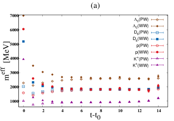
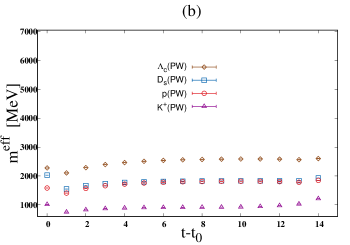
Figure 1: Effective mass plot of $\Lambda_{c},D_{s},p$ and $K^{+}$ for (a) wall-wall (WW) and point-wall (PW), in addition, to have better comparison in the plot (b) only point-wall correlators are shown.

The overlap parameters are used to obtain the $\Lambda_{c}K^{+}-pD_{s}$ coupled channel potentials. They contribute to the $\Lambda_{c}K^{+}-pD_{s}$ coupled channel potential in the combination $\sqrt{\left(Z_{\Lambda_{c}}Z_{K^{+}}\right)/\left(Z_{p}Z_{D_{s}}\right)}$. Here, $Z_{\Lambda_{c}},Z_{K^{+}},Z_{p}$ and $Z_{D_{s}}$ denote the $Z$ factors of local composite hadron operators for $\Lambda_{c},K^{+},p$ and $D_{s}$ hadrons, respectively. The identification plateau regions and the results for the hadron masses are given in Table 1, whereas these values leads to $\sqrt{\left(Z_{\Lambda_{c}}Z_{K^{+}}\right)/\left(Z_{p}Z_{D_{s}}\right)}=1.22$.

Table 1: Hadron masses in unit of MeV. Statistical errors are shown in the parentheses.

The $Z_{H}$ is defined in Eq. (15) and the $Z_{p}$ is the Z-factor of proton. Hadron $\sqrt{Z_{H}}$ $\sqrt{\frac{Z_{H}}{Z_{p}}}$ $m_{H}\left[\textrm{MeV}\right]$ Fit Range $m_{exp}[\textrm{MeV}]$ $\pi$ $872(3)$ $6-10$ $135$ $K$ $1.478(7)$ $6.234$ $910(1)$ $5-10$ $493.67$ $p$ $0.2371(2)$ $1.000$ $1810(3)$ $7-12$ $938.27$ $D_{s}$ $1.81(1)$ $7.662$ $1825(1)$ $7-11$ $1968.30$ $\Lambda_{c}$ $0.3569(9)$ $1.505$ $2583(3)$ $8-12$ $2286.46$

IV.2 Time dependence

First, we investigate the time dependence of the diagonal potentials. The time interval $t-t_{0}=8\pm 1$ is selected to suppress contribution from higher excited states at smaller $t$ and simultaneously to avoid large statistical errors at larger $t$ [22]. Fig. 2 shows $V_{\Lambda_{c}K^{+}}^{\Lambda_{c}K^{+}}$ and $V_{pD_{s}}^{pD_{s}}$ at three values of $t-t_{0}=7,8,9$. Based on the time-dependent HAL QCD method [32], within statistical errors, no significant $t-t_{0}$ dependence is observed for these potentials showing that $t-t_{0}=8$ is large enough to suppress inelastic contributions and that higher-order contributions in the derivative expansion are negligible.

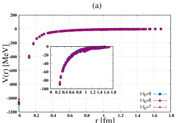
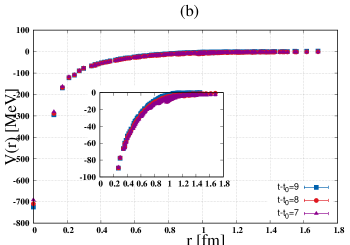
Figure 2: Time dependences of the diagonal potentials matrix, panel (a) for $V_{\Lambda_{c}K^{+}}^{\Lambda_{c}K^{+}}$ and panel (b) for $V_{pD_{s}}^{pD_{s}}$ as function of $r$ at $t-t_{0}=7$ (darkmagenta), $8$ (red) and $9$ (blue).

IV.3 Potentials

The numerical results of the S-wave $\Lambda_{c}K^{+}-pD_{s}$ coupled-channel potential matrix are presented in Fig 3. This figure shows attractions at all distances without repulsive core for diagonal elements of the potential matrix $V_{\Lambda_{c}K^{+}}^{\Lambda_{c}K^{+}}$ and $V_{pD_{s}}^{pD_{s}}$, and the attraction at short distance $\left(r<0.5\right)$ fm in the $\Lambda_{c}K^{+}$ channel is stronger than in the $pD_{s}$ channel. These (diagonal and off-diagonal) potentials, almost vanish at $r>1$ fm.

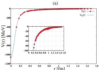
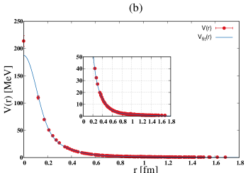
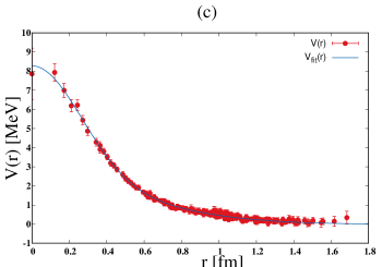
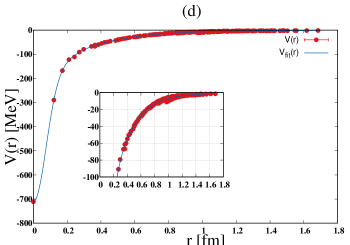
Figure 3: The S-wave $\Lambda_{c}K^{+}-pD_{s}$ coupled-channel potential matrix (red circle). The solid blue line is the corresponding fitted function. The time separation between sink and source is $t-t_{0}=8$. Panels show elements of the potential matrix, (a) $V_{\Lambda_{c}K^{+}}^{\Lambda_{c}K^{+}}$, (b) $V_{\Lambda_{c}K^{+}}^{pD_{s}}$, (c) $V_{pD_{s}}^{\Lambda_{c}K^{+}}$ and (d) $V_{pD_{s}}^{pD_{s}}$, respectively.

IV.4 Hermiticity

Hermiticity of the potential matrix is a sufficient condition for the probability conservation, though it is not a necessary condition. Furthermore, the Hermiticity of the potential matrix is not automatically guaranteed in the definition of the coupled-channel potential matrix in Eq. (2). From Fig. 3 it is apparent that the Hermiticity is largely broken, i.e. the off-diagonal parts of the potential (panel (b) and (c) in Fig. 3) matrix are different. This may indicate that it could be better to include the $pD_{s}^{\ast}$ channel into our calculation. To treat this broken Hermiticity, we have done further analysis. Solving the coupled-channel Schrödinger equation with non-Hermitian potential is problematic because the unitarity of the S-matrix is not guaranteed. Therefore, it is common to apply Hermitian potential in phenomenological studies in nuclear physics. Since this broken Hermiticity is happened at short distances, the low energy scattering observables does not suffer from difference between $V_{\Lambda_{c}K^{+}}^{pD_{s}}$ and $V_{pD_{s}}^{\Lambda_{c}K^{+}}$. In order to check this the coupled channel potential is made Hermitian by taking one of them for the off-diagonal part or their average,

$$\bar{V}_{\Lambda_{c}K^{+}}^{pD_{s}}=\left(V_{\Lambda_{c}K^{+}}^{pD_{s}}+V_{pD_{s}}^{\Lambda_{c}K^{+}}\right)/2.$$ (16)

In Appendix A, it is shown clearly that the scattering phase shifts of ${\Lambda_{c}K}$ and ${pD_{s}}$ for the above $3$ Hermitian potential cases are almost same within the statistical errors. Thus hereafter we consider the $\bar{V}_{\Lambda_{c}K^{+}}^{pD_{s}}$ in our calculations.

V Analytic forms of ${\Lambda_{c}K^{+}}$ and ${pD_{s}}$ potentials

In order to use the LQCD potential in phenomenological investigations, it is useful to fit them with some functions. Accordingly for the diagonal (D) ${\Lambda_{c}K^{+}}-{\Lambda_{c}K^{+}}$ $\left(V_{\Lambda_{c}K^{+}}^{\Lambda_{c}K^{+}}\right)$, ${pD_{s}}-{pD_{s}}$ $\left(V_{pD_{s}}^{pD_{s}}\right)$ potentials as presented in Fig. 3, the following fit function $V_{D}\left(r\right)$ is considered [37, 38],

$$V_{\textrm{D}}\left(r\right)={\displaystyle\sum_{i=1}^{3}\alpha_{i}e^{-\beta_{i}r^{2}}}+\lambda\left[\mathcal{Y}\left(\rho,m_{\pi},r\right)\right]^{2},$$ (17)

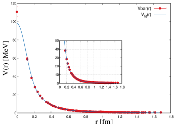
Figure 4: Hermitian (average) potential, $\bar{V}_{\Lambda_{c}K^{+}}^{pD_{s}}$ in Eq. (16) and its fit function at $t-t_{0}=8$.

And similarly for the off-diagonal(OD) $\bar{V}_{\Lambda_{c}K^{+}}^{pD_{s}}$ as presented in Fig. 4, the following analytic form $V_{\textrm{OD}}\left(r\right)$ is selected [39],

$$V_{\textrm{OD}}\left(r\right)={\displaystyle\sum_{i=1}^{3}\alpha_{i}e^{-\beta_{i}r^{2}}},$$ (18)

where $\mathcal{Y}$ is the Yukawa function with a form factor,

$$\mathcal{Y}\left(\rho,m_{\pi},r\right)\equiv\left(1-e^{-\rho r^{2}}\right)\frac{e^{-m_{\pi}r}}{r}.$$ (19)

In the Eq. (17), the $\mathcal{Y}$ form, at medium and long range distances is motivated by the picture of two-pion exchange. The Gauss form factors in the Eq. (17) and (18) describe the short range part of the potentials. Note that the pion mass $m_{\pi}$ are fixed to be the measured values on the lattice about $872$ MeV.

The results of fit and corresponding parameters are given in Table 2 for $V_{\Lambda_{c}K^{+}}^{\Lambda_{c}K^{+}}$, Table 3 for $V_{pD_{s}}^{pD_{s}}$ and Table 4 for $\bar{V}_{\Lambda_{c}K^{+}}^{pD_{s}}$ at three different values $t-t_{0}=7,8,9$.

Table 2: Fitted parameters in Eq. (17) for $V_{\Lambda_{c}K^{+}}^{\Lambda_{c}K^{+}}$ with statistical errors using the data at $r<1.7$ fm. $\alpha_{i},\beta_{i}$ and $\rho$ are given in units of $\left[\textrm{MeV}\right],\left[\textrm{fm}^{-2}\right]$ and $\left[\textrm{fm}^{-2}\right]$, respectively.

	Gauss-1			Gauss-2			Gauss-3			${\textrm{Yukawa}}^{2}$
$t-t_{0}$	$\alpha_{1}$	$\beta_{1}$		$\alpha_{2}$	$\beta_{2}$		$\alpha_{3}$	$\beta_{3}$		$\lambda$	$\rho$
$7$	$-953.3(4.0)$	$106.4(2.2)$		$-51.8(2.7)$	$3.4(4)$		$-12.2(4.1)$	$0.635(230)$		$-31.0(2.0)$	$36.5(2.5)$
$8$	$-990.3(6.5)$	$106.6(3.2)$		$-52.9(2.6)$	$3.9(6)$		$-15.2(5.0)$	$0.791(251)$		$-32.9(2.8)$	$36.5(3.4)$
$9$	$-1011.6(8.6)$	$109.8(3.0)$		$-57.4(2.4)$	$4.0(4)$		$-13.2(4.2)$	$0.766(253)$		$-32.8(2.1)$	$39.2(3.0)$

Table 3: Fitted parameters in Eq. (17) for $V_{pD_{s}}^{pD_{s}}$ with the statistical errors using the data at $r<1.7$ fm. Units are the same as those in Table 2.

	Gauss-1			Gauss-2			Gauss-3			${\textrm{Yukawa}}^{2}$
$t-t_{0}$	$\alpha_{1}$	$\beta_{1}$		$\alpha_{2}$	$\beta_{2}$		$\alpha_{3}$	$\beta_{3}$		$\lambda$	$\rho$
$7$	$-604.5(4.2)$	$98.0(1.6)$		$-74.4(2.2)$	$3.9(4)$		$-13.4(5.6)$	$0.848(340)$		$-24.8(4.4)$	$25.0(2.9)$
$8$	$-621.5(3.9)$	$98.3(1.5)$		$-74.8(2.6)$	$4.1(4)$		$-14.5(5.8)$	$0.947(350)$		$-25.2(3.9)$	$25.9(2.7)$
$9$	$-630.2(3.6)$	$103.5(1.8)$		$-78.6(3.5)$	$4.6(4)$		$-17.9(5.7)$	$1.1(3)$		$-19.0(2.0)$	$33.9(3.0)$

Table 4: Fitted parameters in Eq. (16) for Hermitian $\bar{V}_{\Lambda_{c}K^{+}}^{pD_{s}}$ potential with the statistical errors using the data at $r<1.7$ fm. Units are the same as those in Table 2.

	Gauss-1			Gauss-2			Gauss-3
$t-t_{0}$	$\alpha_{1}$	$\beta_{1}$		$\alpha_{2}$	$\beta_{2}$		$\alpha_{3}$	$\beta_{3}$
$7$	$72.8(1.5)$	$52.9(1.9)$		$23.2(1.5)$	$8.0(5)$		$2.8(4)$	$0.629(133)$
$8$	$71.8(4.7)$	$45.9(4.3)$		$23.6(2.1)$	$7.8(9)$		$2.8(9)$	$0.959(300)$
$9$	$83.1(3.4)$	$55.6(4.8)$		$27.2(2.4)$	$8.7(1.3)$		$4.1(1.6)$	$1.4(4)$

VI Phase shift and scattering length

The physical observables such as coupled-channel scattering phase shifts of $\Lambda_{c}K^{+}-pD_{s}$ interactions can be calculated. Therefore, we solve the coupled-channel Schrödinger equation with the fitted potentials (given in the previous section) in the infinite volume and extract S- matrix from the asymptotic behaviour of the wave functions. Here the convention introduced by Stapp et al. [40] is used for the definition of phase shifts in the case of coupled channel system as

$$\left(\begin{array}[]{cc}S_{\Lambda_{c}K^{+}}^{\Lambda_{c}K^{+}}&S_{\Lambda_{c}K^{+}}^{pD_{s}}\\ S_{pD_{s}}^{\Lambda_{c}K^{+}}&S_{pD_{s}}^{pD_{s}}\end{array}\right)=$$ (20)

$$\left(\begin{array}[]{cc}e^{i\bar{\delta}_{\Lambda_{c}K^{+}}}&0\\ 0&e^{i\bar{\delta}_{pD_{s}}}\end{array}\right)\left(\begin{array}[]{cc}\cos 2\bar{\epsilon}&i\sin 2\bar{\epsilon}\\ i\sin 2\bar{\epsilon}&\cos 2\bar{\epsilon}\end{array}\right)\left(\begin{array}[]{cc}e^{i\bar{\delta}_{\Lambda_{c}K^{+}}}&0\\ 0&e^{i\bar{\delta}_{pD_{s}}}\end{array}\right),$$

where $\bar{\delta}$ is so-called the bar phase shift and $\bar{\epsilon}$ is the mixing angle.

At first, since it is desired to see how large the coupled channel effect, we have compared the single channel ${\Lambda_{c}K^{+}}$ potential and a diagonal part of the coupled channel potential, i.e., $V_{\Lambda_{c}K^{+}}^{\Lambda_{c}K^{+}}$ at $t-t_{0}=8$ (panel (a) in Fig 5) and their corresponding scattering phase shifts (panel (b) in Fig 5) below $pD_{s}$ threshold $(W_{CN}\simeq 157\textrm{MeV})$ as well. By using the single channel potential and solving the Schrödinger equation, it is established that the single channel potential does not have a bound state.

Panel (a) and panel (b) in Fig. 6, shows resultant S-wave scattering phase shifts for $\Lambda_{c}K^{+}$ and $pD_{s}$ channels as a function of the baryon-meson center-of-mass energy, respectively. The $\Lambda_{c}K$ phase-shift shows a weak attraction. Moreover, just above the $\Lambda_{c}K$ threshold the $S$-wave phase shift shows a rapid variation, a feature indicative of a nearby pole. However, at the opening of the $pD_{s}$ threshold we do observe a noticeable “kink” in the $\Lambda_{c}K$ phase shift suggesting a non-zero coupling between the two channels. The coupled $\Lambda_{c}K$, $pD_{s}$ system, showing an enhancement (steadily increasing) in the $\Lambda_{c}K$ phase shift. The non-zero coupling between channels is further demonstrated in Fig. 6, panel (c), which shows a clear deviation of the inelasticities, $\eta$ from unity. The inelasticity indicates that the transition between the $\Lambda_{c}K^{+}$ and $pD_{s}$ is weak and two channels are almost independent each other. This observation might be understood from the fact that the large mass splitting between the $\Lambda_{c}K^{+}$ and $pD_{s}$.

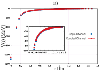
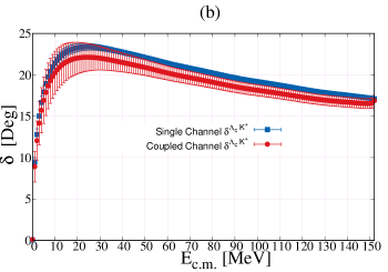
Figure 5: Panel (a) shows a comparison between the single channel ${\Lambda_{c}K^{+}}$ potential (blue square) and a diagonal part of the coupled channel potential (red circle), and panel (b) presents the relevant phase shifts in the single and coupled channel at $t-t_{0}=8$. The mild difference between single and coupled channel phase shift is due to the effect of coupled channel. The $\Lambda_{c}K^{+}$ phase shift are plotted against the energies from the $\Lambda_{c}K^{+}$ threshold. In the case of single channel $\Lambda_{c}K^{+}$ potential the corresponding fit parameters are given by Table. 5 in Appendix B.

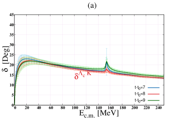
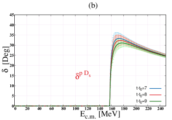
Figure 6: The phase shifts of S-wave (a) $\Lambda_{c}K^{+}$, (b) $pD_{s}$ and (c) the inelasticity of the scattering defined as $\eta=\left|S_{\Lambda_{c}K^{+}}^{\Lambda_{c}K^{+}}\right|=\left|\cos 2\bar{\epsilon}\right|$ is plotted against the energies from the $\Lambda_{c}K^{+}$ threshold for $t-t_{0}=7$ (blue), $8$ (red) and $9$ (green).

As mentioned above, because the two channels are almost independent each other due to the small mixing, they can be regarded as two single channels, therefore, from the low-energy part of $\Lambda_{c}K^{+}\left(pD_{s}\right)$ phase shifts in Fig. 6 (a) ((b)) the scattering length $\left(a_{0}\right)$ and the effective range $\left(r_{\textrm{eff}}\right)$ are derived by using the S-wave effective range expansion (ERE) up to the next-to-leading order (NLO),

$$k\>\cot\delta=-\frac{1}{a_{0}}+\frac{1}{2}r_{\textrm{eff}}k^{2}+\mathcal{O}\left(k^{4}\right),$$ (21)

The results are

$$\begin{array}[]{cc}a_{0}^{\Lambda_{c}K^{+}}=-0.87\pm 0.19_{-0.12}^{+0.06}\>\textrm{fm},&r_{\textrm{eff}}^{\Lambda_{c}K^{+}}=2.60\pm 0.26_{-0.22}^{+0.03}\>\textrm{fm},\end{array}$$ (23)

$$\begin{array}[]{cc}a_{0}^{pD_{S}}=-1.42\pm 0.36_{-0.17}^{+0.18}\>\textrm{fm},&r_{\textrm{eff}}^{pD_{S}}=1.74\pm 0.19_{-0.06}^{+0.07}\>\textrm{fm},\end{array}$$ (25)

where the central values and the statistical errors are evaluated at $t-t_{0}=8$, while the systematic errors are evaluated by the difference between the central values at $t-t_{0}$ and those at $t-t_{0}=7$ and $9$.

In addition, because the electric charge of each hadron in the $\Lambda_{c}K^{+}-pD_{s}$ system is $+e$ we have Coulomb repulsion. It is probably too early to consider Coulomb interaction since the pion mass in our simulation is as heavy as $872$ MeV, therefor for future lattice QCD simulation at physical point (with nearly physical quark mass, i.e., $m_{\pi}\simeq 146$ MeV and $m_{K}\simeq 525\textrm{MeV}$) [41], it is necessary to include Coulomb interaction.

VII Summary and conclusion

We have investigated the S-wave $\Lambda_{c}K^{+}$ interaction using the $\Lambda_{c}K^{+}-pD_{s}$ coupled channel potentials obtained by the extension of the HAL QCD method in Flavor $\textrm{SU}\left(3\right)$ Limit of Lattice QCD. Results of the potential matrix show that the diagonal elements, $\Lambda_{c}K^{+}$ and $pD_{s}$ are both strongly attractive, while, $\Lambda_{c}K^{+}$ has a much deeper attractive pocket than $pD_{s}$. We have also observed weak off-diagonal elements of the potential matrix. They are not Hermitician, which is not guaranteed from the definition. The phase shifts and inelasticity extracted by solving Schrödinger equation in the infinite volume with the obtained potentials show that the $\Lambda_{c}K^{+}$ channel does not have the two-body bound state at $m_{\pi}\geq 872$ MeV. While the inelasticity (mixing angle between $\Lambda_{c}K^{+}$ and $pD_{s}$ channel also indicates a small coupling between the two. the coupled $\Lambda_{c}K$, $pD_{s}$ system, showing an enhancement (steadily increasing) in the $\Lambda_{c}K$ phase shift.

And last but not the least, since in one hand the $pD_{s}^{*}$ threshold is quite close to the kinematic region considered, and on the other hand, the mass difference between $D_{s}$ ($1968.30$ MeV) and $D_{s}^{*}$ ($2112.1$ MeV) is about $143.8$ MeV, therefore, in future it is necessary to carry out full channel coupling analysis with $pD_{s}^{*}$ by using $\left(2+1\right)$-flavor and $\left(1+1+1\right)$-flavor lattice simulation at physically quark masses $\left(m_{\pi}\approx 138\>\textrm{MeV}\right)$ on a sufficient large lattice.

Appendix A Dependence on different off-diagonal potentials

Since the Hermiticity is broken at short distances, the low energy scattering observables does not suffer from difference between $V_{\Lambda_{c}K^{+}}^{pD_{s}}$ and $V_{pD_{s}}^{\Lambda_{c}K^{+}}$. We have checked this by performing the following analysis. We first made the coupled channel potential Hermitian (an average or take one of them for the off-diagonal part). We then performed the analysis with coupled channel potential even above the threshold to check the observable difference among all 4 following cases of the off-diagonal part (one non-Hermitian and three Hermitian)

(a) Non-Hermitian, (b) Average of off-diagonal part i.e., $\bar{V}_{\Lambda_{c}K^{+}}^{pD_{s}}$, (c) $V_{12}=V_{21}=V_{\Lambda_{c}K^{+}}^{pD_{s}}$, (d) $V_{12}=V_{21}=V_{pD_{s}}^{\Lambda_{c}K^{+}}$. The scattering phase shifts of ${\Lambda_{c}K}$ and ${pD_{s}}$ and the relevant inelasticity parameter for the above $4$ cases are presented and compared in panel (a), (b) and (c) of Fig. 7, respectively.

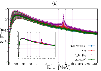
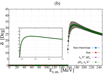
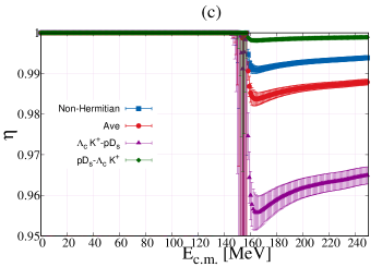
Figure 7: The scattering phase shifts of S-wave (a) $\Lambda_{c}K^{+}$, (b) $pD_{s}$ and (c) the inelasticity parameter correspond to the phase shifts calculated with non-Hermitian (blue), $\bar{V}_{\Lambda_{c}K^{+}}^{pD_{s}}$ (red), $V_{\Lambda_{c}K^{+}}^{pD_{s}}$ (purple) and $V_{pD_{s}}^{\Lambda_{c}K^{+}}$ (green) at $t-t_{0}=8$.

Appendix B Fitted parameters for single channel $\Lambda_{c}K^{+}$ potential

The analytic form same as Eq. (17) also is used for single channel $\Lambda_{c}K^{+}$ potential. The resultant fit parameters are given in Table. 5. The scattering phase shift which obtained by these parameters for $t-t_{0}=8$, is presented in Fig. 5, panel (b).

Table 5: Fitted parameters in Eq. (17) for single channel $\Lambda_{c}K^{+}$ potential with statistical errors using the data at $r<1.7$ fm. $\alpha_{i},\beta_{i}$ and $\rho$ are given in units of $\left[\textrm{MeV}\right],\left[\textrm{fm}^{-2}\right]$ and $\left[\textrm{fm}^{-2}\right]$, respectively.

	Gauss-1			Gauss-2			Gauss-3			${\textrm{Yukawa}}^{2}$
$t-t_{0}$	$\alpha_{1}$	$\beta_{1}$		$\alpha_{2}$	$\beta_{2}$		$\alpha_{3}$	$\beta_{3}$		$\lambda$	$\rho$
$7$	$-632.7(3.0)$	$102.5(2.0)$		$-44.6(1.2)$	$3.42(27)$		$-14.5(2.3)$	$0.47(10)$		$-24.6(1.8)$	$31.9(2.2)$
$8$	$-1027.5(7.5)$	$106.0(3.0)$		$-56.6(2.3)$	$4.02(51)$		$-16.1(4.8)$	$0.80(23)$		$-32.9(2.8)$	$36.5(3.4)$
$9$	$-1048.6(8.8)$	$108.4(4.2)$		$-61.2(2.2)$	$4.01(411)$		$-13.9(4.2)$	$0.76(0.24)$		$-36.2(2.5)$	$37.6(3.0)$

References

- Brambilla et al. [2020] N. Brambilla et al., The XYZ states: Experimental and theoretical status and perspectives, Phys. Rep. 873, 1 (2020).
- Guo et al. [2018] F.-K. Guo et al., Hadronic molecules, Rev. Mod. Phys. 90, 015004 (2018).
- Aaij et al. [2022] R. Aaij et al., Study of the doubly charmed tetraquark , Nat. Commun. 13, 3351 (2022).
- Ikeda et al. [2016] Y. Ikeda et al. (HAL QCD Collaboration), Fate of the Tetraquark Candidate from Lattice QCD, Phys. Rev. Lett. 117, 242001 (2016).
- Lyu et al. [2023] Y. Lyu, S. Aoki, T. Doi, T. Hatsuda, Y. Ikeda, and J. Meng, Doubly Charmed Tetraquark from Lattice QCD near Physical Point, Phys. Rev. Lett. 131, 161901 (2023).
- Aaij et al. [2019] R. Aaij et al. (LHCb Collaboration), Observation of a Narrow Pentaquark State, , and of the Two-Peak Structure of the , Phys. Rev. Lett. 122, 222001 (2019).
- Acharya et al. [2022] S. Acharya et al. (ALICE Collaboration), First study of the two-body scattering involving charm hadrons, Phys. Rev. D 106, 052010 (2022).
- Yasui and Sudoh [2013] S. Yasui and K. Sudoh, Heavy-quark dynamics for charm and bottom flavor on the fermi surface at zero temperature, Phys. Rev. C 88, 015201 (2013).
- Hattori et al. [2015] K. Hattori, K. Itakura, S. Ozaki, and S. Yasui, Qcd kondo effect: Quark matter with heavy-flavor impurities, Phys. Rev. D 92, 065003 (2015).
- Suenaga et al. [2022] D. Suenaga, Y. Araki, K. Suzuki, and S. Yasui, Heavy-quark spin polarization induced by the kondo effect in a magnetic field, Phys. Rev. D 105, 074028 (2022).
- Kondo [1964] J. Kondo, Resistance Minimum in Dilute Magnetic Alloys, Prog. Theor. Phys. 32, 37 (1964).
- Hewson [1993] A. C. Hewson, The Kondo Problem to Heavy Fermions, Cambridge Studies in Magnetism (Cambridge University Press, 1993).
- Yasui [2016] S. Yasui, Kondo effect in charm and bottom nuclei, Phys. Rev. C 93, 065204 (2016).
- Yasui and Miyamoto [2019] S. Yasui and T. Miyamoto, Spin-isospin kondo effects for and baryons and and mesons, Phys. Rev. C 100, 045201 (2019).
- Yasui and Sudoh [2017] S. Yasui and K. Sudoh, Kondo effect of and mesons in nuclear matter, Phys. Rev. C 95, 035204 (2017).
- Yamaguchi et al. [2022] Y. Yamaguchi, S. Yasui, and A. Hosaka, Open charm and bottom meson-nucleon potentials à la the nuclear force, Phys. Rev. D 106, 094001 (2022).
- Aoki and Doi [2020] S. Aoki and T. Doi, Lattice QCD and Baryon-Baryon Interactions: HAL QCD Method, Front. Phys. 8 (2020).
- Epelbaum et al. [2009] E. Epelbaum, H.-W. Hammer, and U.-G. Meißner, Modern theory of nuclear forces, Rev. Mod. Phys. 81, 1773 (2009).
- Ishii et al. [2007] N. Ishii, S. Aoki, and T. Hatsuda, Nuclear Force from Lattice QCD, Phys. Rev. Lett. 99, 022001 (2007).
- Aoki et al. [2012] S. Aoki et al. (HAL QCD Collaboration), Lattice quantum chromodynamical approach to nuclear physics, Prog. Theor. Exp. Phys. 2012 (2012), 01A105.
- Aoki et al. [2013] S. Aoki et al. (HAL QCD Collaboration), Construction of energy-independent potentials above inelastic thresholds in quantum field theories, Phys. Rev. D 87, 034512 (2013).
- Sasaki et al. [2015] K. Sasaki et al. (HAL QCD Collaboration), Coupled-channel approach to strangeness S=-2 baryon-baryon interaction in lattice QCD, Prog. Theor. Exp. Phys. 2015 (2015), 113B01.
- Sasaki et al. [2020] K. Sasaki et al. (HAL QCD Collaboration), and interactions from lattice near the physical point, Nucl. Phys. A 998, 121737 (2020).
- Miyamoto et al. [2018] T. Miyamoto et al. (HAL QCD Collaboration), interaction from lattice QCD and its application to hypernuclei, Nucl. Phys. A 971, 113 (2018).
- Lyu et al. [2021] Y. Lyu et al., Dibaryon with Highest Charm Number near Unitarity from Lattice QCD, Phys. Rev. Lett. 127, 072003 (2021).
- Ikeda et al. [2014] Y. Ikeda et al. (HAL QCD Collaboration), Charmed tetraquarks and from dynamical lattice QCD simulations, Phys. Lett. B 729, 85 (2014).
- Akahoshi et al. [2021] Y. Akahoshi, S. Aoki, and T. Doi, Emergence of the resonance from the HAL QCD potential in lattice QCD, Phys. Rev. D 104, 054510 (2021).
- Ikeda et al. [2011] Y. Ikeda et al., Structure of (1405) and threshold behavior of scattering, Prog. Theor. Phys. 125, 1205 (2011).
- Murakami et al. [2023] K. Murakami et al. (HAL QCD Collaboration), Lattice quantum chromodynamics (QCD) studies on decuplet baryons as meson–baryon bound states in the HAL QCD method, Prog. Theor. Exp. Phys. 2023, 043B05 (2023).
- Iritani et al. [2016] T. Iritani et al. (HAL QCD Collaboration), Mirage in temporal correlation functions for baryon-baryon interactions in lattice QCD, J. High Energy Phys. 2016 (10), 1.
- Iritani et al. [2017] T. Iritani et al. (HAL QCD Collaboration), Are two nucleons bound in lattice QCD for heavy quark masses? Consistency check with Lüscher’s finite volume formula, Phys. Rev. D 96, 034521 (2017).
- Ishii et al. [2012] N. Ishii et al., Hadron–hadron interactions from imaginary-time Nambu–Bethe–Salpeter wave function on the lattice, Phys. Lett. B 712, 437 (2012).
- [33] CP-PACS/JLQCD Collaborations, Available at https://www.jldg.org/ildg-data/CPPACS+JLQCDconfig.html.
- Ishikawa et al. [2008] T. Ishikawa et al. (CP-PACS and JLQCD Collaborations), Light-quark masses from unquenched lattice QCD, Phys. Rev. D 78, 011502 (2008).
- [35] Japan Lattice Data Grid (JLDG), Available athttp://www.lqcd.org/ildg and http://www.jldg.org.
- Can et al. [2013] K. Can, G. Erkol, B. Isildak, M. Oka, and T. Takahashi, Electromagnetic properties of doubly charmed baryons in Lattice QCD, Phys. Lett. B 726, 703 (2013).
- Etminan et al. [2014] F. Etminan et al. (HAL QCD Collaboration), Spin-2 dibaryon from lattice , Nucl. Phys. A 928, 89 (2014), special Issue Dedicated to the Memory of Gerald E Brown (1926-2013).
- Iritani et al. [2019] T. Iritani et al. (HAL QCD Collaboration), dibaryon from lattice near the physical point, Phys. Lett. B 792, 284 (2019).
- Gongyo et al. [2018] S. Gongyo et al. (HAL QCD Collaboration), Most Strange Dibaryon from Lattice , Phys. Rev. Lett. 120, 212001 (2018).
- Stapp et al. [1957] H. P. Stapp, T. J. Ypsilantis, and N. Metropolis, Phase-Shift Analysis of 310-Mev Proton-Proton Scattering Experiments, Phys. Rev. 105, 302 (1957).
- [41] K. I. Ishikawa et al. (PACS Collaboration), 2+1 Flavor QCD Simulation on a Lattice, PoS LATTICE2015, 075, arXiv:1511.09222 [hep-lat] .