Fast Minimization of Expected Logarithmic Loss via
Stochastic Dual Averaging

Abstract

Consider the problem of minimizing an expected logarithmic loss over either the probability simplex or the set of quantum density matrices. This problem encompasses tasks such as solving the Poisson inverse problem, computing the maximum-likelihood estimate for quantum state tomography, and approximating positive semi-definite matrix permanents with the currently tightest approximation ratio. Although the optimization problem is convex, standard iteration complexity guarantees for first-order methods do not directly apply due to the absence of Lipschitz continuity and smoothness in the loss function.

In this work, we propose a stochastic first-order algorithm named $B$-sample stochastic dual averaging with the logarithmic barrier. For the Poisson inverse problem, our algorithm attains an $\varepsilon$-optimal solution in $\smash{\tilde{O}}(d^{2}/\varepsilon^{2})$ time, matching the state of the art. When computing the maximum-likelihood estimate for quantum state tomography, our algorithm yields an $\varepsilon$-optimal solution in $\smash{\tilde{O}}(d^{3}/\varepsilon^{2})$ time, where $d$ denotes the dimension. This improves on the time complexities of existing stochastic first-order methods by a factor of $d^{\omega-2}$ and those of batch methods by a factor of $d^{2}$, where $\omega$ denotes the matrix multiplication exponent. Numerical experiments demonstrate that empirically, our algorithm outperforms existing methods with explicit complexity guarantees.

1 Introduction

Denote by $\mathscr{D}_{d}$ the set of $d\times d$ quantum density matrices, i.e., the set of Hermitian positive semi-definite (PSD) matrices of unit traces. Let $P$ be a distribution over the set of $d\times d$ Hermitian PSD matrices. Consider the optimization problem of minimizing an expected logarithmic loss:

$$f^{\star}=\min_{\rho\in\mathscr{D}_{d}}f(\rho),\quad f(\rho)\coloneqq\mathbb{E}_{A\sim P}[-\log\operatorname*{tr}(A\rho)].$$ (1)

A point $\hat{\rho}\in\mathscr{D}_{d}$ is said to be $\varepsilon$-optimal if $f(\hat{\rho})-f^{\star}\leq\varepsilon$. When both $A$ and $\rho$ are restricted to diagonal matrices, the optimization problem (1) reduces to

$$\min_{x\in\Delta_{d}}f(x),\quad f(x)\coloneqq\mathbb{E}_{a\sim P^{\prime}}[-\log\braket{a,x}]$$ (2)

where $\Delta_{d}$ denotes the probability simplex in $\mathbb{R}^{d}$ and $P^{\prime}$ is a distribution over $[0,\infty)^{d}$. We refer to the two problems (1) and (2) as the quantum setup and the classical setup, respectively. For the special cases when

$$\begin{split}f(\rho)&\coloneqq\frac{1}{n}\sum_{i=1}^{n}-\log\operatorname*{tr}(A_{i}\rho),\ \text{or}\\ f(x)&\coloneqq\frac{1}{n}\sum_{i=1}^{n}-\log\braket{a_{i},x},\end{split}$$

we say the optimization problems are in the finite-sum setting with sample size $n$.

Notably, the classical setup (2) encompasses the problem of computing Kelly’s criterion, an asymptotically optimal strategy in long-term investment [1, 2, 3]. It is also equivalent to solving the Poisson inverse problem, which finds applications in positron emission tomography (PET) in medical imaging and astronomical image denoising [4, 5]. Lastly, the problem is the batch counterpart of the online portfolio selection problem [6], for which designing algorithms that are optimal in both regret and computational complexity has remained unsolved for over thirty years [7, 8].

The quantum setup (1) has even broader applications. One important example is computing the maximum-likelihood (ML) estimate for quantum state tomography [9], a fundamental task for the verification of quantum devices. Another example is computing a semidefinite programming relaxation of the PSD matrix permanents [10]. The relaxation achieves the currently tightest approximation ratio and can be used to estimate the output probabilities of Boson sampling experiments [11].

Although the optimization problems (1, 2) are convex, standard convex optimization methods face two challenges. The first challenge is the lack of Lipschitz continuity and smoothness in the loss function [12]. As a result, iteration complexity guarantees of standard first-order methods, such as mirror descent and dual averaging, do not directly apply [13, 14]. While second-order methods, such as Newton’s method, do possess explicit complexity guarantees [13], they still face the second challenge.

The second challenge is the scalabilities with respect to the dimension $d$ and sample size $n$ in the finite-sum setting. For instance, the dimension $d$ typically reaches millions, and the sample size $n$ can exceed hundreds of millions in PET [15, 16]. Both $d$ and $n$ grow exponentially with the number of qubits (quantum bits) in quantum state tomography [17]. However, the per-iteration time complexities of batch methods grow at least linearly with $n$, and those of second-order methods scale poorly with $d$ as they require computing Hessian inverses.

When dealing with high dimensionality and large sample sizes, stochastic first-order algorithms, such as stochastic gradient descent, are preferred. Their per-iteration time complexities can be independent of the sample size $n$, and they do not require computationally demanding operations involving Hessian matrices. Nevertheless, standard stochastic first-order algorithms continue to face the challenge related to the lack of Lipschitz continuity and smoothness, as mentioned earlier.

Due to the absence of Lipschitz continuity and smoothness, mini-batch stochastic Q-Soft-Bayes (SQSB) [18, 19] and stochastic Q-LB-OMD (SQLBOMD) [20, 21] are the only two stochastic first-order methods with clear time complexity guarantees for solving the problems (1, 2). Both algorithms do not compete with batch methods in terms of the empirical convergence speed, as shown in Section 6. Stochastic mirror descent studied by D’Orazio et al. [22] is only guaranteed to solve the problems up to an arbitrarily large error. Other stochastic first-order methods, such as stochastic primal-dual hybrid gradient (SPDHG) [23, 24], stochastic mirror-prox [25], and stochastic coordinate descent [26], are only guaranteed to converge asymptotically.

Contributions

In this work, we propose a mini-batch stochastic first-order algorithm named $B$-sample stochastic dual averaging with the logarithmic barrier (LB-SDA, Algorithm 1) for solving the optimization problems (1, 2), where $B$ denotes the mini-batch size. The expected optimization error of $B$-sample LB-SDA vanishes at a rate of $\smash{\tilde{O}}(d/t+\sqrt{d/(Bt)})$. This matches the standard results of mini-batch stochastic gradient descent for minimizing smooth functions [27], regardless of the absence of smoothness in our problem.

In the classical setup, the time complexity of obtaining an $\varepsilon$-optimal solution via $B$-sample LB-SDA is $\smash{\tilde{O}}(d^{2}/\varepsilon^{2})$, matching the state of the art of stochastic first-order methods [19, 20]. In the quantum setup, the time complexity of obtaining an $\varepsilon$-optimal solution is $\smash{\tilde{O}}(d^{3}/\varepsilon^{2})$ when the mini-batch size is set to $d$. This improves the dimension dependence of existing stochastic algorithms by a factor of $d^{\omega-2}$, where $\omega\in[2,2.372)$ denotes the matrix multiplication exponent [28]. It is worth noting that in practical implementation, such as BLAS [29], $\omega$ is effectively $3$. The time complexity guarantee also improves the sample size dependence of the currently fastest batch algorithm by a factor of $n/d$. Such improvement is significant, given that $n=\Omega(d^{3})$ is necessary for ML quantum state tomography [17].

Lastly, we conducted numerical experiments to demonstrate the efficiency of the proposed method. The numerical results suggest that $1$-sample LB-SDA is the currently fastest method with explicit complexity guarantees for the Poisson inverse problem, and $d$-sample LB-SDA outperforms all methods in terms of fidelity, a standard measure of the closeness of quantum states, for ML quantum state tomography. To the best of our knowledge, this is the first empirical evidence that stochastic first-order algorithms can surpass batch ones in computing the ML estimate for quantum state tomography.

Technical Breakthroughs

Our analysis consists of three key ingredients: a regret bound of Tsai et al. [30], a smoothness characterization of the logarithmic loss (Lemma 4), and a new local-norm-based analysis of the standard online-to-batch conversion [31], all of which are of independent interest.

Tsai et al. [30] proved the following regret bound for online convex optimization with the logarithmic loss on the probability simplex $\Delta_{d}$ (Appendix A.2):

$$R_{t}\leq\smash{\tilde{O}}\left(\sqrt{d\sum_{\tau=1}^{t}\lVert\nabla f_{\tau}(\rho_{\tau})\rVert_{\rho_{\tau},\ast}^{2}}\right)\leq\smash{\tilde{O}}\left(\sqrt{dt}\right),$$ (3)

where $\lVert\cdot\rVert_{\rho,\ast}$ is the dual local norm associated with the logarithmic barrier. Directly applying the standard online-to-batch conversion [31] with the second upper bound can only yield an optimization error bound of $\smash{\tilde{O}}(\sqrt{d/t})$, which is independent of the mini-batch size. In comparison, we make use of the finer first upper bound and derive an optimization error bound of $\tilde{O}(d/t+\sqrt{d/(Bt)})$. This leads to a time complexity bound of $\smash{\tilde{O}}(d^{3}/\varepsilon^{2}+d^{\omega+1}/(B\varepsilon^{2}))$ for the quantum setup, which creates space for improved dimensional scalability via choosing the mini-batch size $B$. See Section 5.3 for a detailed discussion.

To make use of the finer first regret bound (3), we generalize the smoothness characterization of the logarithmic loss of Tsai et al. [30] for the quantum setup. The original proof of Tsai et al. [30] is challenging to generalize due to the noncommutativity in the quantum setup. Our generalization is based on a great simplification of their proof by utilizing self-concordance properties of the logarithmic loss (Appendix A.1).

Our analysis modifies that of the anytime online-to-batch conversion [32] to handle the local norms. It is worth noting that we also adapt the analysis of anytime online-to-batch for the standard one, as the latter has shown better empirical performance.

Notations

We denote the set $\{1,2,\ldots,n\}$ by $\llbracket n\rrbracket$ for a natural number $n\in\mathbb{N}$. We denote the $\ell_{p}$-norm by $\lVert\cdot\rVert_{p}$ for $p\in[1,\infty]$. We denote the sets of $d\times d$ Hermitian matrices, Hermitian PSD matrices, and Hermitian positive definite matrices by $\mathbb{H}^{d}$, $\mathbb{H}_{+}^{d}$, and $\mathbb{H}_{++}^{d}$, respectively. We denote the relative interior of a set $S$ by $\operatorname{ri}S$. We denote the $i$-th entry of a vector $v$ by $v(i)$. We denote the conjugate transpose of a matrix $U$ by $U^{\ast}$. We denote the sum of time-indexed matrices $A_{1},\ldots,A_{t}\in\mathbb{H}^{d}$ by $A_{1:t}$. We define the domain of a function $f:\mathbb{H}^{d}\to\mathbb{R}\cup\{\infty\}$ by $\smash{\operatorname{dom}f\coloneqq\{\rho\in\mathbb{H}^{d}\mid f(\rho)<\infty\}}$.

Algorithms	Iter. complexity	Per-iter. time	Time complexity	References
NoLips	$d/\varepsilon$	$nd^{2}+d^{\omega}$	$(nd^{2}+d^{\omega})/\varepsilon$	Bauschke et al. [33]
QEM	$\log d/\varepsilon$	$nd^{2}+d^{\omega}$	$(nd^{2}+d^{\omega})/\varepsilon$	Lin et al. [18]
Frank-Wolfe	$n/\varepsilon$	$nd^{\omega}$	$n^{2}d^{\omega}/\varepsilon$	Zhao and Freund [34]
SQSB	$d/\varepsilon^{2}$	$d^{\omega}$	$d^{\omega+1}/\varepsilon^{2}$	Lin et al. [19]
SQLBOMD	$d/\varepsilon^{2}$	$d^{\omega}$	$d^{\omega+1}/\varepsilon^{2}$	Tsai et al. [20]
$1$-sample LB-SDA	$d/\varepsilon^{2}$	$d^{\omega}$	$d^{\omega+1}/\varepsilon^{2}$	Corollary 7 (this work)
$d$-sample LB-SDA	$1/\varepsilon^{2}$	$d^{3}$	$d^{3}/\varepsilon^{2}$	Corollary 7 (this work)
$B$-sample LB-SDA	$d/(B\varepsilon^{2})$	$Bd^{2}+d^{\omega}$	$d^{3}/\varepsilon^{2}+d^{\omega+1}/(B\varepsilon^{2})$	Corollary 7 (this work)

Table 1: A comparison of existing first-order methods for the quantum setup (1) with explicit complexity guarantees. Iteration complexity and time complexity refer to the number of iterations and arithmetic operations required to obtain an $\varepsilon$-optimal solution, respectively. We assume $t\gg d^{2}$ and omit logarithmic factors, where $t$ denotes the number of iterations.

2 Related Work

The relationships between this work and the works of Tsai et al. [30] and Cutkosky [32] have been addressed in Section 1. This section focuses on optimization algorithms.

Although standard optimization methods are not suitable for solving the problems (1, 2), several methods with clear complexity guarantees have been proposed in the last decade. Table 1 summarizes existing results. We focus on batch methods as stochastic methods have already been discussed in Section 1.

QEM [18] is the current theoretically fastest batch method that solve the optimization problem (1) with clear complexity guarantees. Its classical counterpart EM was proposed by Shepp and Vardi [35] and Cover [36] independently. While NoLips, QEM, and Frank-Wolfe have clear complexity guarantees, their time complexities scale at least linearly with the sample size, which is undesirable when the sample size is large.

Other batch methods lack explicit complexity guarantees and, as a result, are not comparable to our algorithm. For instance, the convergence rates of proximal gradient methods [37] and several variants of the Frank-Wolfe method [38, 39, 40] involve unknown parameters. Diluted iterative MLE (iMLE) [41, 42] and entropic mirror descent (EMD) with Armijo line search [12] are only guaranteed to converge asymptotically. Additionally, OSEM [43] for PET and iMLE [44] for ML quantum state tomography are commonly used heuristics but do not converge in general [43, 41].

3 Applications

3.1 Kelly’s Criterion

Denote by $\Delta_{d}$ the probability simplex in $\mathbb{R}^{d}$. Consider long-term investment in a market with $d$ investment alternatives. Let $\{a_{t}\}$ be a stochastic process taking values in $[0,\infty)^{d}$. On day $t$, the investor first selects a portfolio $x_{t}\in\Delta_{d}$ that indicates the distribution of their assets among the $d$ investment alternatives. Then, the investor observes $a_{t}$ that provides the price relatives of the investment alternatives for that day. The investor’s goal is to maximize the wealth growth rate.

Kelly’s criterion suggests choosing $x_{t+1}$ by maximizing the expected logarithmic loss conditional on the past, i.e.,

$$x_{t+1}\in\operatorname*{arg\!\min}_{x\in\Delta_{d}}\mathbb{E}_{a_{t+1}}[-\log\braket{a_{t+1},x}\mid a_{1},\ldots,a_{t}],$$

which requires solving the classical setup (2).

3.2 Poisson Inverse Problem

In the Poisson inverse problem, our goal is to recover an unknown signal $\smash{\lambda^{\natural}\in[0,\infty)^{d}}$ based on $n$ independent measurement outcomes $\{y_{i}\}$. Each outcome $y_{i}$ follows a Poisson distribution with mean $\braket{b_{i},\lambda^{\natural}}$, where $b_{i}\in[0,\infty)^{d}$ is known and depends on the measurement setup. In positron emission tomography, $\lambda^{\natural}(i)$ represents the emitter density of the $i$-th region, and $y_{i}$ represents the number of photons detected by the $i$-th sensor.

The ML estimate is given by [35]

$$\hat{\lambda}\in\operatorname*{arg\!\min}_{\lambda\in[0,\infty)^{d}}\sum_{i=1}^{n}(\braket{b_{i},\lambda}-y_{i}\log\braket{b_{i},\lambda}).$$ (4)

Vardi and Lee [4] and Ben-Tal et al. [15] showed that by setting

$$Y=\sum_{i=1}^{n}y_{i},\quad\hat{\lambda}(i)=\frac{Y\hat{x}(i)}{\sum_{j=1}^{n}a_{j}(i)},\quad\forall i\in\llbracket n\rrbracket,$$

and

$$a_{i}(j)=\frac{Yb_{i}(j)}{\sum_{k=1}^{n}b_{k}(j)},\quad\forall i\in\llbracket n\rrbracket,\ j\in\llbracket d\rrbracket,$$

the ML estimate can be reformulated as

$$\hat{x}\in\operatorname*{arg\!\min}_{x\in\Delta_{d}}\sum_{i=1}^{n}-\frac{y_{i}}{Y}\log\braket{a_{i},x},$$

which is equivalent to the classical setup (2) in the finite-sum setting with $\mathbb{P}(a=a_{i})=y_{i}/Y$ for all $i\in\llbracket n\rrbracket$.

3.3 ML Quantum State Tomography

A quantum state is described by a density matrix $\rho\in\mathscr{D}_{d}$, which is a $d\times d$ Hermitian PSD matrix of unit trace. For a state consisting of $q$ qubits, $d$ equals $2^{q}$. Denote by $\mathscr{D}_{d}$ the set of density matrices. The set $\mathscr{D}_{d}$ can be regarded as a quantum generalization of $\Delta_{d}$, in the sense that the vector of eigenvalues of any $\rho\in\mathscr{D}_{d}$ lies in $\Delta_{d}$.

Given $n$ measurement outcomes from an unknown quantum state $\rho^{\natural}$, ML estimation is a standard and widely used approach to estimate $\rho^{\natural}$ [9, 45, 46, 47]. The ML estimate is given by

$$\hat{\rho}_{\text{ML}}\in\operatorname*{arg\!\min}_{\rho\in\mathscr{D}_{d}}\frac{1}{n}\sum_{i=1}^{n}-\log\operatorname*{tr}(A_{i}\rho),$$

for some known $A_{i}\in\mathbb{H}_{+}^{d}$ related to the $i$-th measurement outcome. Note that solving $\hat{\rho}_{\text{ML}}$ requires solving the quantum setup (1) in the finite-sum setting.

3.4 PSD Matrix Permanents

The permanent of a matrix $A\in\mathbb{C}^{d\times d}$ is defined as

$$\operatorname{per}A\coloneqq\sum_{\pi\in S_{d}}\sum_{i=1}^{d}A_{i,\pi(i)},$$

where $S_{d}$ is the set of all permutations of $\llbracket d\rrbracket$. Let $\{v_{i}\}_{i}$ be the eigenvectors of $A$. Yuan and Parrilo [10] proposed the following approximation of $\operatorname{per}A$ when $A\in\mathbb{H}_{+}^{d}$:

$$\operatorname{rel}A\coloneqq\max_{\rho\in\mathscr{D}_{d}}\prod_{i=1}^{d}\operatorname*{tr}((dv_{i}v_{i}^{\ast})\rho).$$

The approximation is equivalent to the quantum setup (1) in the finite-sum setting with $A_{i}=dv_{i}v_{i}^{\ast}$. As noted by Meiburg [48], $\operatorname{rel}A$ achieves the currently tightest approximation ratio of $4.85^{d}$.

4 Characterizations of Logarithmic Loss

This section aims to address the aforementioned lack of Lipschitz continuity and smoothness in the logarithmic loss. We first set up a few notations. For $\rho\in\mathbb{H}_{++}^{d}$, let

$$h(\rho)\coloneqq-\log\det\rho$$ (5)

be the logarithmic barrier. Let $\smash{\lVert\cdot\rVert_{\rho}\coloneqq(D^{2}h(\rho)[\cdot,\cdot])^{1/2}}$ be the local norm associated with $h$ at $\rho\in\operatorname{dom}h$. The following lemma gives explicit formulae for the local norm and its dual norm. The proof is deferred to Appendix B.1.

Lemma 1.

For $\rho\in\mathbb{H}^{d}_{++}$ and $X\in\mathbb{H}^{d}$, the local norm and its dual norm associated with $h$ are given by

$$\begin{split}&\lVert X\rVert_{\rho}=\sqrt{\operatorname*{tr}((\rho^{-1/2}X\rho^{-1/2})^{2})}=\sqrt{\operatorname*{tr}((\rho^{-1}X)^{2})},\\ &\lVert X\rVert_{\rho,\ast}=\sqrt{\operatorname*{tr}((\rho^{1/2}X\rho^{1/2})^{2})}=\sqrt{\operatorname*{tr}((\rho X)^{2})}.\end{split}$$ (6)

4.1 “Lipschitz Continuity”

A continuously differentiable function $f:\mathbb{H}^{d}\to\mathbb{R}$ is said to be $G$-Lipschitz with respect to a norm $\lVert\cdot\rVert$ if its gradients are bounded by $G$ in the dual norm, i.e., $\lVert\nabla f(\rho)\rVert_{\ast}\leq G$.

Although the loss function is not Lipschitz, Lemma 2 below shows that $\nabla f$ is bounded in the dual local norm associated with $h$. This Lipschitz-type property enables us to control the distance between iterates and exploit local properties of the loss function, in particular, the local smoothness property of self-concordant functions (Theorem 11).

Lemma 2 is a simple quantum generalization of Lemma 4.3 of Tsai et al. [30]. Its proof is deferred to Appendix B.2.

Lemma 2.

Let $f$ be defined in the quantum setup (1). Then, $\lVert\nabla f(\rho)\rVert_{\rho,\ast}\leq 1$ for all $\rho\in\mathbb{H}_{++}^{d}$.

4.2 “Smoothness”

A continuously differentiable function $f:\mathbb{H}^{d}\to\mathbb{R}$ is said to be $L$-smooth with respect to a norm $\lVert\cdot\rVert$ if its gradient is $L$-Lipschitz with respect to $\lVert\cdot\rVert$, i.e.,

$$\lVert\nabla f(\rho)-\nabla f(\rho^{\prime})\rVert_{\ast}\leq L\lVert\rho-\rho^{\prime}\rVert,\quad\forall\rho,\rho^{\prime}\in\mathbb{H}^{d}.$$

Lemma 3, known as the self-bounding property, is a consequence of smoothness [49]. A proof of Lemma 3 can be found in Lemma 4.23 of Orabona [50].

Lemma 3.

Let $f:\mathbb{R}^{d}\to\mathbb{R}$ be $L$-smooth with respect to $\lVert\cdot\rVert$ with $\operatorname{dom}f=\mathbb{R}^{d}$. Then, for any $x\in\mathbb{R}^{d}$, it holds that

$$\lVert\nabla f(x)\rVert_{\ast}^{2}\leq 2L\left(f(x)-\inf_{x^{\prime}\in\mathbb{R}^{d}}f(x^{\prime})\right).$$

Although the loss function is not smooth, Lemma 4 below establishes a self-bounding-type property of the loss function. As discussed in Section 1, the lemma generalizes Lemma 4.7 of Tsai et al. [30] to the quantum setup, and greatly simplifies the proof therein. The proof is deferred to Appendix B.3.

For any $\rho\in\operatorname{ri}\mathscr{D}_{d}$ and $X\in\mathbb{H}^{d}$, define

$$\alpha_{\rho}(X)\coloneqq-\frac{\operatorname*{tr}(\rho X\rho)}{\operatorname*{tr}(\rho^{2})}\in\operatorname*{arg\!\min}_{\alpha\in\mathbb{R}}\lVert X+\alpha I\rVert_{\rho,\ast}^{2}.$$ (7)

Lemma 4.

Let $f$ be defined in the quantum setup (1). Then, for any $\rho\in\operatorname{ri}\mathscr{D}_{d}$, it holds that

$$\lVert\nabla f(\rho)+\alpha_{\rho}(\nabla f(\rho))I\rVert_{\rho,\ast}^{2}\leq 4\left(f(\rho)-\min_{\rho^{\prime}\in\mathscr{D}_{d}}f(\rho^{\prime})\right).$$

5 Algorithms and Convergence Guarantees

This section presents LB-SDA and its theoretical guarantee. We focus on the quantum setup (1) since it includes the classical setup (2) as a special case.

5.1 Algorithm

LB-SDA is presented in Algorithm 1, where $h$ is the logarithmic barrier (5) and $\lVert\cdot\rVert_{\rho}$ and $\lVert\cdot\rVert_{\rho,\ast}$ are the local norm and the dual local norm associated with $h$ at $\rho$ (6), respectively. A stochastic first-order oracle is a randomized function $\mathcal{O}$ that outputs an unbiased estimate $\mathcal{O}(\rho)\in\mathbb{H}^{d}$ of the gradient $\nabla f(\rho)$ given an input $\rho\in\mathscr{D}_{d}$.

Algorithm 1 Stochastic Dual Averaging with the Logarithmic Barrier (LB-SDA) for the quantum setup (1)

Input: A sequence of learning rates $\{\eta_{t}>0\mid t\in\mathbb{N}\}$ and a stochastic first-order oracle $\mathcal{O}$.

1:$h(\rho)\coloneqq-\log\det\rho$.

2:$\rho_{1}=I/d\in\operatorname*{arg\!\min}_{\rho\in\mathscr{D}_{d}}h(\rho)$.

3:for all $t\in\mathbb{N}$ do

4:   Output $\bar{\rho}_{t}\coloneqq(1/t)\rho_{1:t}$.

5:   $g_{t}=\mathcal{O}(\rho_{t})$.

6:   $\smash{\rho_{t+1}\in\operatorname*{arg\!\min}_{\rho\in\mathscr{D}_{d}}\eta_{t}\operatorname*{tr}(g_{1:t}\rho)+h(\rho)}$.

7:end for

We will make the following assumptions on the stochastic first-order oracle. It is notable that the boundedness is defined in terms of the dual local norm, which deviates from existing literature.

Assumption 1.

Conditional on the past, the stochastic gradients $\{g_{t}\}$ in Algorithm 1 are unbiased and bounded, and their variances are also bounded, i.e., for all $t\in\mathbb{N}$,

• $\mathbb{E}[g_{t}|\mathcal{H}_{t}]=\nabla f(\rho_{t})$,

• ${\mathbb{E}\left[\lVert g_{t}\rVert_{\rho_{t},\ast}^{2}\big{|}\mathcal{H}_{t}\right]\leq G^{2}}$,

• ${\mathbb{E}\left[\lVert g_{t}-\nabla f(\rho_{t})\rVert_{\rho_{t},\ast}^{2}\big{|}\mathcal{H}_{t}\right]\leq\sigma^{2}}$,

where $\mathcal{H}_{t}=\{g_{1},\ldots,g_{t-1},\rho_{1},\ldots,\rho_{t}\}$ is the past information before obtaining $g_{t}$.

The unbiasedness and bounded variance assumptions are standard in the literature. Regarding the bounded gradient assumption, by the triangle inequality and Lemma 2,

$$\begin{split}\lVert g_{t}\rVert_{\rho_{t},\ast}^{2}&\leq(\lVert g_{t}-\nabla f(\rho_{t})\rVert_{\rho_{t},\ast}+\lVert\nabla f(\rho_{t})\rVert_{\rho_{t},\ast})^{2}\\ &\leq\lVert g_{t}-\nabla f(\rho_{t})\rVert_{\rho_{t},\ast}^{2}+2\lVert g_{t}-\nabla f(\rho_{t})\rVert_{\rho_{t},\ast}+1.\end{split}$$

Taking expectations on both sides and using the inequality $\mathbb{E}X\leq\sqrt{\mathbb{E}[X^{2}]}$, we can verify that the bounded gradient assumption always holds with $G=1+\sigma$. Nevertheless, since $G$ can be smaller than $1+\sigma$, we include the assumption for a tighter result.

An important example of the oracle is

$$\mathcal{O}_{B}(\rho)\coloneqq\frac{1}{B}\sum_{b=1}^{B}\nabla\ell_{b}(\rho)$$ (8)

where $B\in\mathbb{N}$, $\ell_{b}(\rho)\coloneqq-\log\operatorname*{tr}(A_{b}\rho)$, and $A_{1},\ldots,A_{B}$ are independently drawn from $P$. The resulting algorithm is called $B$-sample LB-SDA. The following lemma justifies the use of $\mathcal{O}_{B}$, whose proof is deferred to Appendix B.4.

Lemma 5.

The oracle $\mathcal{O}_{B}$ (8) satisfies Assumption 1 with $G=1$ and $\sigma^{2}=4/B$.

5.2 Convergence Guarantee

The non-asymptotic convergence guarantee of Algorithm 1 is presented in Theorem 6 below. The analysis follows the online-to-batch approach, where we use the following regret bound of Tsai et al. [30] in Appendix A.2:

$$R_{t}\leq\smash{\tilde{O}}\left(\sqrt{d\sum_{\tau=1}^{t}\lVert g_{\tau}+\alpha_{\rho_{\tau}}(g_{\tau})I\rVert_{\rho_{\tau},\ast}^{2}}\right)\leq\smash{\tilde{O}}(\sqrt{dt}).$$

Note that applying the online-to-batch conversion on the right upper bound can only yield a convergence rate of $\smash{\tilde{O}}(\sqrt{d/t})$, independent of the variance $\sigma^{2}$. Since the effect of batch size is unclear without the variance term, the direct approach fails to improve the time complexity guarantee.

Deriving the variance term typically requires smoothness of the loss function in the literature, and this is where the self-bounding-type property (Lemma 4) comes into play. It bounds the square of the dual local norm by

$$\mathbb{E}\lVert g_{\tau}+\alpha_{\rho_{\tau}}(g_{\tau})I\rVert_{\rho_{\tau},\ast}^{2}\leq 4\mathbb{E}[f(\rho_{\tau})-\min_{\rho^{\prime}\in\mathscr{D}_{d}}f(\rho^{\prime})]+\sigma^{2},$$

which results in a “self-bounding” inequality of $\mathbb{E}R_{t}$:

$$\mathbb{E}R_{t}\leq\smash{\tilde{O}}\left(\sqrt{d\mathbb{E}R_{t}+\sigma^{2}dt}\right)$$

Our analysis can be seen as a local-norm extension of that of the anytime online-to-batch conversion [32]. The proof is deferred to Appendix B.5.

Theorem 6.

Consider the quantum setup (1). Under Assumption 1, let $\{\bar{\rho}_{t}\}$ be the iterates generated by Algorithm 1 with

$$\eta_{t}=\frac{\sqrt{d}}{\sqrt{\sum_{\tau=1}^{t}\lVert g_{\tau}+\alpha_{\rho_{\tau}}(g_{\tau})I\rVert_{\rho_{\tau},\ast}^{2}+4dG^{2}+G^{2}}}.$$

Then, for all $t\in\mathbb{N}$, it holds that

$$\begin{split}&\mathbb{E}\left[f(\bar{\rho}_{t})-\min_{\rho\in\mathscr{D}_{d}}f(\rho)\right]\\ &\qquad\leq\frac{4dC_{t}^{3}+2C_{t}\sqrt{\sigma^{2}dt+4d^{2}G^{2}+dG^{2}}+1}{t}\\ &\qquad=O\left(\frac{dG(\log t)^{3}}{t}+\frac{\sigma\sqrt{d}\log t}{\sqrt{t}}\right),\end{split}$$

where $C_{t}\coloneqq\log t+3$ and the expectation is taken with respect to $\{g_{t}\}$.

Plugging in the estimates in Lemma 5, we obtain the following result for the mini-batch case.

Corollary 7.

Consider the quantum setup (1). Let $\{\bar{\rho}_{t}\}$ be the iterates of B-sample LB-SDA with learning rates

$$\eta_{t}=\frac{\sqrt{d}}{\sqrt{\sum_{\tau=1}^{t}\lVert g_{\tau}+\alpha_{\rho_{\tau}}(g_{\tau})I\rVert_{\rho_{\tau},\ast}^{2}+4d+1}}.$$

Then, for all $t\in\mathbb{N}$, it holds that

$$\mathbb{E}\left[f(\bar{\rho}_{t})-\min_{\rho\in\mathscr{D}_{d}}f(\rho)\right]=O\left(\frac{d(\log t)^{3}}{t}+\frac{\sqrt{d}\log t}{\sqrt{Bt}}\right).$$

where the expectation is taken with respect to $\{g_{t}\}$.

Remark 8.

Proving high-probability guarantees for $B$-sample LB-SDA is challenging since the logarithmic loss violates the boundedness assumption required by standard analysis [50]. We left this extension as a future research direction.

5.3 Time Complexity Analysis

This section discusses the time complexity of $B$-sample LB-SDA and compares it with existing methods. Comparisons of time complexities of existing first-order methods has been presented in Table 1 and discussed in Section 1.

First, note that the 6th line in Algorithm 1 cannot be solved exactly. Nevertheless, after an eigendecomposition, which takes $\smash{\tilde{O}}(d^{\omega})$ time [51], the 6th line reduces to an one-dimensional convex optimization problem, which can be efficiently solved by Newton’s method on the real line in $\smash{\tilde{O}}(d)$ time (see, e.g., Appendix A.2 of Nesterov [13]). As a result, the time complexity of the 6th line is $\smash{\tilde{O}}(d^{\omega})$. Second, the time complexity of the 5th line, which requires implementing the oracle $\mathcal{O}_{B}$, is $O(Bd^{2})$. Lastly, since the 5th and the 6th lines are the most time-consuming parts, the per-iteration time complexity of $B$-sample LB-SDA is $O(Bd^{2}+d^{\omega})$.

By Corollary 7, the iteration complexity of $B$-sample LB-SDA to obtain an $\varepsilon$-optimal solution is $\smash{\tilde{O}}(d/(B\varepsilon^{2}))$. Combining with the per-iteration time complexity, the overall time complexity is $\smash{\tilde{O}}(d^{3}/\varepsilon^{2}+d^{\omega+1}/(B\varepsilon^{2}))$. In particular, the overall time complexity is $\smash{\tilde{O}}(d^{3}/\varepsilon^{2})$ when $B=\Omega(d^{\omega-2})$. Since $\omega$ is $3$ in practical implementation [29], we will often choose $B=d$.

Since the eigendecomposition is no longer needed in the classical setup, the per-iteration time complexity of $B$-sample LB-SDA is reduced to $\smash{\tilde{O}}(Bd)$. Because the iteration complexity of obtaining an $\varepsilon$-optimal solution is $\smash{\tilde{O}}(d/(B\varepsilon^{2}))$, the overall time complexity is $\smash{\tilde{O}}(d^{2}/\varepsilon^{2})$ for any $B\in\mathbb{N}$ in the classical setup.

6 Numerical Results

We have shown that LB-SDA achieves the currently best time complexity guarantees in the previous section. In this section, we show that LB-SDA also performs well empirically. We consider solving the Poisson inverse problem and computing the ML estimate for quantum state tomography. All results in this section are presented in terms of the elapsed time. Results in terms of the number of iterations can be found in Appendix C.

Both experiments were conducted on a machine with an Intel Xeon Gold 5218 CPU of 2.30GHz and 131,621,512kB memory. The elapsed time records the actual running time of the method on the machine. All methods are implemented in the Julia programming language [52] with the Intel Math Kernel Library, and the number of threads in BLAS is set to $8$. It is important to note that the empirical speed is highly dependent on the specific implementations.

The approximate optimization error at an iterate is defined as the difference between its function value and the smallest one obtained in the experiments.

6.1 Poisson Inverse Problem

Consider the Poisson inverse problem in Section 3.2 with a synthetic dataset, where $d$ equals $256$ and $n$ equals $1,000,000$. The unknown signal $\lambda^{\natural}$ is the gray intensities of the Shepp-Logan phantom image [53] of size $16\times 16$ multiplied by $1,000$. The signal is presented in Appendix C. The vectors $\{b_{i}\}$ are generated following the scheme of Raginsky et al. [54]. Each entry of $b_{i}$ is assigned to either $0$ or $1/n$ with equal probability.

We consider all algorithms in Table 1 that have explicit complexity guarantees. EM [35], SSB [55], and SLBOMD [20] are the classical counterparts of QEM, SQSB, and SQLBOMD, respectively. Additionally, we include SPDHG [23] and EMD with Armijo line search [56] for comparison. The former is well-known in practice and the latter is known to converge fast empirically. However, they are only guaranteed to converge asymptotically. Their parameters are set according to the cited works. We do not include batch PDHG as it is slow in practice.

We solve the Poisson inverse problem based on the equivalence between it and the classical setup (2) in Section 3.2. Figure 1 presents the numerical results. For an iterate $\hat{\lambda}$, the normalized estimation error is defined as $\lVert\hat{\lambda}-\lambda^{\natural}\rVert_{2}/\lVert\lambda^{\natural}\rVert_{2}$. Since the goal of the Poisson inverse problem is to recover the unknown signal $\lambda^{\natural}$, rather than minimizing the loss function, results presented in terms of the normalized estimation error is more important than results presented in terms of the optimization error.

Observe that $1$-sample LB-SDA outperforms all methods with explicit complexity guarantees in terms of the normalized estimation error. Although it is slower than EMD with line search and SPDHG, the latter two methods are only guaranteed to converge asymptotically, whereas LB-SDA has an explicit non-asymptotic complexity guarantee.

LB-SDA converges faster than SLBOMD and SSB in terms of the optimization error, although they have the same theoretical time complexity of $\smash{\tilde{O}}(d^{2}/\varepsilon^{2})$. This can be explained by the use of time-varying learning rates in LB-SDA, in contrast to the fixed learning rates used by the other two methods. The time-varying learning rates are large in the beginning, which leads to a fast convergence in practice.

Figure 1: Performances of all algorithms in Table 1, SPDHG, and EMD with line search for solving the Poisson inverse problem.

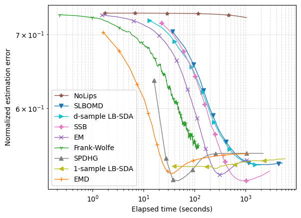
(a) Normalized estimation error versus the elapsed time.

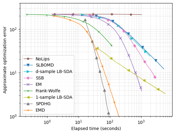
(b) Approximate optimization error versus the elapsed time.

6.2 ML Quantum State Tomography

Consider the problem of ML quantum state tomography in Section 3.3. We construct a synthetic dataset, following the setup of Häffner et al. [45]. The number of qubits $q$ is $6$, the dimension $d$ is $2^{6}=64$, and the sample size $n$ is $409,600$. The unknown quantum state is the $W$ state, which corresponds to a rank-$1$ density matrix. The Hermitian matrices $\{A_{i}\}$ are generated following the procedure of Lin et al. [18], where each $A_{i}$ is of rank $d/2$.

We compare all algorithms in Table 1, along with iMLE [44], diluted iMLE [42], and EMD with Armijo line search [56]. Their parameters are set according to the cited works. Although iMLE does not always converge [41], we include it because it is often considered as a benchmark. We do not include the accelerated projected gradient descent [57] as it is slower than iMLE in experiments [58].

Figure 2: Performances of all algorithms in Table 1, iMLE, diluted iMLE, and EMD with line search for computing the ML estimate for quantum state tomography.

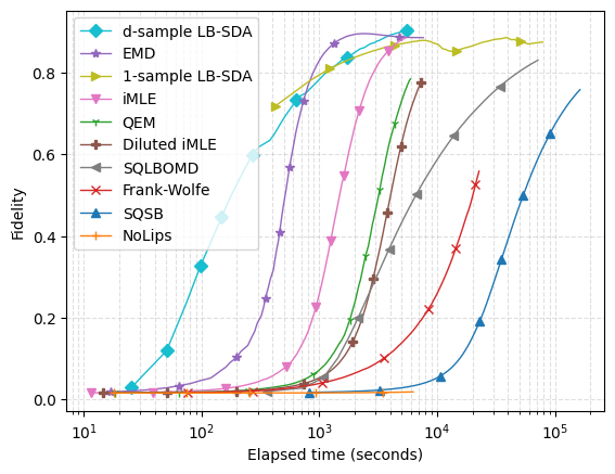
(a) Fidelity between the iterates and the $W$ state versus the elapsed time.

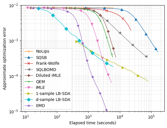
(b) Approximate optimization error versus the elapsed time.

Figure 2 presents the numerical results. The fidelity between two quantum states $\rho,\rho^{\prime}\in\mathscr{D}_{d}$ is defined as $\smash{F(\rho,\rho^{\prime})\coloneqq\left(\operatorname*{tr}\sqrt{\sqrt{\rho}\rho^{\prime}\sqrt{\rho}}\right)^{2}}\in[0,1]$. It is a standard measure of the closeness of two quantum states, with $F(\rho,\rho^{\prime})=1$ if and only if $\smash{\rho=\rho^{\prime}}$. Similar to the Poisson inverse problem, as the goal of quantum state tomography is to recover the unknown quantum state, results presented in terms of the fidelity is more important than results presented in terms of the optimization error.

Observe that $d$-sample outperforms all methods in terms of the fidelity. We conclude that $d$-sample LB-SDA achieves the currently best theoretical time complexity and the currently best empirical performance.

Note that $d$-sample LB-SDA performs better than SQLBOMD and SQSB in terms of the optimization error. It also outperforms QEM and diluted iMLE when the optimization error is not smaller than $10^{-3}$. Recall that the time complexity of QEM has a worse dimension dependence and a better optimization error dependence than that of $d$-sample LB-SDA, and diluted iMLE lacks a non-asymptotic complexity guarantee. Although $d$-sample LB-SDA is slower than EMD with line search and iMLE in terms of the optimization error, the latter two methods lack clear complexity results.

While it is theoretically known that stochastic methods outperform batch ones when the dimension and the sample size are sufficiently large [59], empirical results presented in the literature did not confirm this phenomenon. In this work, we observed that $d$-sample LB-SDA outperforms all methods in terms of the fidelity. This marks the first empirical evidence that stochastic methods can be more efficient than batch methods for computing the ML estimate for quantum state tomography.

7 Concluding Remarks

We have proposed a stochastic first-order method named $B$-sample LB-SDA for solving the Poisson inverse problem, computing the ML estimate for quantum state tomography, and approximating PSD matrix permanents. In particular, $d$-sample LB-SDA takes $\smash{\tilde{O}}(d^{3}/\varepsilon^{2})$ time to obtain an $\varepsilon$-optimal solution in the quantum setup, improving the time complexities of existing first-order methods. The improvement is based on a new analysis for mini-batch methods, which relies on a novel self-bounding-type property of the logarithmic loss and a new local-norm based analysis of the online-to-batch conversion. Lastly, we have shown that LB-SDA performs better empirically than all methods with explicit complexity guarantees.

Several research directions arise. One direction is to design accelerated or variance-reduced methods for solving the optimization problem (1) based on the smoothness characterization. Another direction is to generalize our argument to other non-smooth loss functions.

Appendix A Preliminaries

Throughout this section, let $(\mathbb{V},\braket{\cdot,\cdot})$ be a finite-dimensional real Hilbert space, such as $\mathbb{R}^{d}$ with the standard inner product and $\mathbb{H}^{d}$ with the Hilbert-Schmidt inner product $\braket{U,V}\coloneqq\operatorname*{tr}(U^{\ast}V)$. Let $\mathcal{X}\subseteq\mathbb{V}$ be a convex set.

A.1 Self-Concordance and Relative Smoothness

This section provides necessary background information on the notions of self-concordance [60, 13] and relative smoothness [33, 61], which form the basis of the smoothness characterization in Section 4. We begin with self-concordance. Define $\omega(t)\coloneqq t-\log(1+t)$ and its Fenchel conjugate $\omega_{\ast}(t)=-t-\log(1-t)$.

Definition 9 (Self-concordance [13]).

A closed convex function $\varphi:\mathbb{V}\to(-\infty,\infty]$ with an open domain $\operatorname{dom}\varphi$ is said to be $M$-self-concordant if it is three-times continuously differentiable on $\operatorname{dom}\varphi$ and

$$\lvert D^{3}\varphi(x)[u,u,u]\rvert\leq 2M(D^{2}\varphi(x)[u,u])^{3/2},\quad\forall x\in\operatorname{dom}\varphi,\ u\in\mathbb{V}.$$

Theorem 10 (Theorem 5.1.5 of Nesterov [13]).

Let $\varphi$ be an $M$-self-concordant function. Let $\lVert\cdot\rVert_{x}\coloneqq(D^{2}\varphi(x)[\cdot,\cdot])^{1/2}$ be the local norm associated with $\varphi$ at $x$. Define the Dikin ellipsoid $W(x)\coloneqq\{y\in\mathbb{V}\mid\lVert y-x\rVert_{x}<1/M\}$. Then, $W(x)\subseteq\operatorname{dom}\varphi$ for all $x\in\operatorname{dom}\varphi$.

Theorem 11 is an important local smoothness-type property of self-concordant functions.

Theorem 11 (Theorem 5.1.9 and Lemma 5.1.5 of [13]).

Let $\varphi$ be an $M$-self-concordant function. Let $\lVert\cdot\rVert_{x}\coloneqq(D^{2}\varphi(x)[\cdot,\cdot])^{1/2}$ be the local norm associated with $\varphi$ at $x$. Then, for $x,y\in\operatorname{dom}\varphi$ such that $\lVert y-x\rVert_{x}<1/M$, it holds that

$$\varphi(y)\leq\varphi(x)+\braket{\nabla\varphi(x),y-x}+\frac{1}{M^{2}}\omega_{\ast}(M\lVert y-x\rVert_{x}).$$

Moreover, if $\lVert y-x\rVert_{x}<1/(2M)$, then

$$\varphi(y)\leq\varphi(x)+\braket{\nabla\varphi(x),y-x}+\lVert y-x\rVert_{x}^{2}.$$

Lemma 12 (Proposition 5.4.5 of Nesterov and Nemirovskii [60]).

The logarithmic barrier $h(\rho)=-\log\det\rho$ is $1$-self-concordant.

Now we introduce the notion of relative smoothness.

Definition 13 (Lu et al. [61]).

Let $f,h:\mathbb{V}\to(-\infty,\infty]$. $f$ is said to be $L$-smooth relative to $h$ on $\mathcal{X}$ for some $L>0$ if $Lh-f$ is convex on $\mathcal{X}$.

Lemma 14 (Proposition 7 of Tsai et al. [62]).

Let $f(\rho)\coloneqq\mathbb{E}[-\log\operatorname*{tr}(A\rho)]$ and $h(\rho)\coloneqq-\log\det\rho$ be the logarithmic barrier. Then, $f$ is $1$-smooth relative to $h$ on $\mathbb{H}_{++}^{d}$.

A.2 FTRL with Self-Concordant Regularizer

This section presents the regret bound of follow-the-regularized-leader (FTRL) with self-concordant regularizers of Tsai et al. [30] in a slightly general form. An online linear optimization problem is a multi-round game between two players, say Learner and Reality. In the $t$-th round,

• first, Learner announces an action $x_{t}\in\mathcal{X}$;

• then, Reality reveals a loss function $f_{t}(x)\coloneqq\braket{v_{t},x}$ for some $v_{t}\in\mathbb{V}$;

• lastly, Learner suffers a loss $f_{t}(x_{t})$.

The goal of Learner is to minimize the regret $\sup_{x\in\mathcal{X}}R_{t}(x)$, defined as

$$R_{t}(x)\coloneqq\sum_{\tau=1}^{t}f_{\tau}(x_{\tau})-\sum_{\tau=1}^{t}f_{\tau}(x),\quad\forall x\in\mathcal{X}.$$

We refer readers to the lecture notes of Orabona [50] and Hazan [63] for a general introduction to online convex optimization.

Algorithm 2 FTRL for online linear optimization

Input: A sequence of learning rates $\{\eta_{t}>0\mid t\in\mathbb{N}\}$.

1:$x_{1}\in\operatorname*{arg\!\min}_{x\in\mathcal{X}}\eta_{0}^{-1}\varphi(x)$.

2:for all $t\in\mathbb{N}$ do

3:   Announce $x_{t}$ and receive $v_{t}\in\mathbb{V}$.

4:   $x_{t+1}\leftarrow\operatorname*{arg\!\min}_{x\in\mathcal{X}}\braket{v_{1:t},x}+\eta_{t}^{-1}\varphi(x)$.

5:end for

FTRL is presented in Algorithm 2. We assume that the regularizer $\varphi$ is a self-concordant function.

Assumption 2.

The function $\varphi$ is an $M$-self-concordant function such that $\mathcal{X}$ is contained in the closure of $\operatorname{dom}\varphi$ and $\min_{x\in\mathcal{X}}\varphi(x)=0$. The Hessian $\nabla^{2}\varphi(x)$ is positive definite for all $x\in\mathcal{X}\cap\operatorname{dom}\varphi$.

Let $\lVert\cdot\rVert_{x}\coloneqq(D^{2}\varphi(x)[\cdot,\cdot])^{1/2}$ be the local norm associated with $\varphi$ at $x$ and $\lVert\cdot\rVert_{x,\ast}$ be its dual norm. The theorem below bounds the regret of Algorithm 2.

Theorem 15 (Theorem 3.2 of Tsai et al. [30]).

Assume that Assumption 2 holds and $\eta_{t-1}\lVert v_{t}\rVert_{x_{t},\ast}\leq 1/(2M)$ for all $t\in\mathbb{N}$. Then, Algorithm 2 satisfies

$$R_{t}(x)\leq\frac{\varphi(x)}{\eta_{t}}+\sum_{\tau=1}^{t}\eta_{\tau-1}\lVert v_{\tau}\rVert_{x_{\tau},\ast}^{2},\quad\forall t\in\mathbb{N}.$$

Remark 16.

It is important to notice that the regret analysis of Tsai et al. [30] directly extends for the quantum setup.

The following corollary has appeared in the proof of Theorem 6.2 of Tsai et al. [30] implicitly. We provide the statement and the proof for completeness.

Corollary 17.

Assume that Assumption 2 holds. Moreover, assume that $\lVert v_{t}\rVert_{x_{t},\ast}\leq G$ for all $t\in\mathbb{N}$. Then, for any $D>0$, Algorithm 2 with

$$\eta_{t}=\frac{D}{\sqrt{\sum_{\tau=1}^{t}\lVert v_{\tau}\rVert_{x_{\tau},\ast}^{2}+4M^{2}G^{2}D^{2}+G^{2}}},\quad\forall t\in\mathbb{N},$$

satisfies

$$R_{t}(x)\leq\left(\frac{\varphi(x)}{D}+2D\right)\sqrt{\sum_{\tau=1}^{t}\lVert v_{\tau}\rVert_{x_{\tau},\ast}^{2}+4M^{2}G^{2}D^{2}+G^{2}},\quad\forall t\in\mathbb{N}.$$

Proof.

First, the learning rates satisfy $\eta_{t-1}\lVert v_{t}\rVert_{x_{t},\ast}\leq 1/(2M)$ for all $t\in\mathbb{N}$ because

$$\eta_{t-1}\lVert v_{t}\rVert_{x_{t},\ast}=\frac{D\lVert v_{t}\rVert_{x_{t},\ast}}{\sqrt{\sum_{\tau=1}^{t-1}\lVert v_{\tau}\rVert_{x_{\tau},\ast}^{2}+4M^{2}G^{2}D^{2}+G^{2}}}\leq\frac{DG}{\sqrt{4M^{2}G^{2}D^{2}}}=\frac{1}{2M}.$$

By Theorem 15 and Lemma 4.13 of Orabona [50], we have

$$\begin{split}R_{t}(x)&\leq\frac{\varphi(x)}{D}\sqrt{\sum_{\tau=1}^{t}\lVert v_{\tau}\rVert_{x_{\tau},\ast}^{2}+4M^{2}G^{2}D^{2}+G^{2}}+D\sum_{\tau=1}^{t}\frac{\lVert v_{\tau}\rVert_{x_{\tau},\ast}^{2}}{\sqrt{\sum_{s=1}^{\tau-1}\lVert v_{s}\rVert_{x_{s},\ast}^{2}+4M^{2}G^{2}D^{2}+G^{2}}}\\ &\leq\frac{\varphi(x)}{D}\sqrt{\sum_{\tau=1}^{t}\lVert v_{\tau}\rVert_{x_{\tau},\ast}^{2}+4M^{2}G^{2}D^{2}+G^{2}}+D\sum_{\tau=1}^{t}\frac{\lVert v_{\tau}\rVert_{x_{\tau},\ast}^{2}}{\sqrt{\sum_{s=1}^{\tau}\lVert v_{s}\rVert_{x_{s},\ast}^{2}}}\\ &\leq\frac{\varphi(x)}{D}\sqrt{\sum_{\tau=1}^{t}\lVert v_{\tau}\rVert_{x_{\tau},\ast}^{2}+4M^{2}G^{2}D^{2}+G^{2}}+2D\sqrt{\sum_{\tau=1}^{t}\lVert v_{\tau}\rVert_{x_{\tau},\ast}^{2}}\\ &\leq\left(\frac{\varphi(x)}{D}+2D\right)\sqrt{\sum_{\tau=1}^{t}\lVert v_{\tau}\rVert_{x_{\tau},\ast}^{2}+4M^{2}G^{2}D^{2}+G^{2}}.\end{split}$$

This completes the proof. ∎

A.3 Online-to-Batch Conversion

This section recaps the online-to-batch conversion proposed by Cesa-Bianchi et al. [31]. Consider the following optimizaiton problem:

$$\min_{x\in\mathcal{X}}f(x),$$

with a stochastic first-order oracle $\mathcal{O}$ that returns an unbiased estimate $\mathcal{O}(x)\in\mathbb{V}$ of $\nabla f(x)$ given any $x\in\mathcal{X}$. Algorithm 3 presents the online-to-batch conversion and Theorem 18 presents its theoretical guarantee.

Algorithm 3 Online-to-batch conversion

Input: An online learning algorithm $\mathcal{A}$.

1:Get $x_{1}$ from $\mathcal{A}$.

2:for all $t\in\mathbb{N}$ do

3:   Output $\bar{x}_{t}\coloneqq(1/t)x_{1:t}$.

4:   $g_{t}=\mathcal{O}(x_{t})$.

5:   Send $f_{t}(x)\coloneqq\braket{g_{t},x}$ to $\mathcal{A}$.

6:   Get $x_{t+1}$ from $\mathcal{A}$.

7:end for

Theorem 18.

Let $R_{t}(x)$ be the regret of the online algorithm $\mathcal{A}$ against $x\in\mathcal{X}$. Assume that the stochastic gradients are unbiased, i.e., $\mathbb{E}[g_{t}|g_{1},\ldots,g_{t-1},x_{1},\ldots,x_{t}]=\nabla f(x_{t})$. Then, for any $x\in\mathcal{X}$, Algorithm 3 satisfies

$$\mathbb{E}\left[f(\bar{x}_{t})-f(x)\right]\leq\frac{\mathbb{E}[R_{t}(x)]}{t},\quad\forall t\in\mathbb{N},$$

and

$$\mathbb{E}\left[\sum_{\tau=1}^{t}(f(\bar{x}_{\tau})-f(x))\right]\leq(1+\log t)\max_{1\leq\tau\leq t}\mathbb{E}[R_{\tau}(x)],\quad\forall t\in\mathbb{N},$$

where $R_{t}(x)\coloneqq\sum_{\tau=1}^{t}\braket{g_{\tau},x_{\tau}-x}$ is the regret, and the expectation is taken with respect to the stochastic gradients $\{g_{t}\}$.

In Theorem 18, the first inequality can be found in Theorem 3.1 of Orabona [50], and the second inequality follows immediately by summing the first one over $t$.

Appendix B Proofs

B.1 Local Norm and Dual Local Norm

Lemma 19.

The local norm $\lVert\cdot\rVert_{\rho}$ is given by $\lVert X\rVert_{\rho}=\sqrt{\operatorname*{tr}((\rho^{-1}X)^{2})}$.

Proof.

By Appendix A.4.1 of Boyd and Vandenberghe [64] and Example 3.20 of Hiai and Petz [65], we write

$$\begin{split}\lVert X\rVert_{\rho}^{2}&=D^{2}h(\rho)[X,X]\\ &=\frac{\mathrm{d}^{2}}{\mathrm{d}t^{2}}-\log\det(\rho+tX)\bigg{\rvert}_{t=0}\\ &=\frac{\mathrm{d}}{\mathrm{d}t}-\operatorname*{tr}((\rho+tX)^{-1}X)\bigg{\rvert}_{t=0}\\ &=\operatorname*{tr}\left(-\frac{\mathrm{d}}{\mathrm{d}t}(\rho+tX)^{-1}\bigg{\rvert}_{t=0}X\right)\\ &=\operatorname*{tr}(\rho^{-1}X\rho^{-1}X).\end{split}$$

The lemma follows. ∎

Lemma 20.

The dual norm of $\lVert\cdot\rVert_{\rho}$ is given by $\lVert X\rVert_{\rho,\ast}=\sqrt{\operatorname*{tr}((\rho X)^{2})}$.

Proof.

By the definition of dual norm,

$$\lVert X\rVert_{\rho,\ast}=\sup_{\lVert\tau\rVert_{\rho}=1}\lvert\operatorname*{tr}(X\tau)\rvert=\sup_{\lVert\tau\rVert_{\rho}=1}\lvert\operatorname*{tr}(\rho^{1/2}X\rho^{1/2}\rho^{-1/2}\tau\rho^{-1/2})\rvert.$$

By the Cauchy-Schwarz inequality and $\lVert\tau\rVert_{\rho}=1$, we have

$$\lvert\operatorname*{tr}(\rho^{1/2}X\rho^{1/2}\rho^{-1/2}\tau\rho^{-1/2})\rvert\leq\sqrt{\operatorname*{tr}((\rho^{1/2}X\rho^{1/2})^{2})\operatorname*{tr}((\rho^{-1/2}\tau\rho^{-1/2})^{2})}=\sqrt{\operatorname*{tr}((\rho^{1/2}X\rho^{1/2})^{2})}.$$

Then,

$$\sup_{\lVert\tau\rVert_{\rho}=1}\lvert\operatorname*{tr}(X\tau)\rvert\leq\sup_{\lVert\tau\rVert_{\rho}=1}\sqrt{\operatorname*{tr}((\rho^{1/2}X\rho^{1/2})^{2})}=\sqrt{\operatorname*{tr}((\rho^{1/2}X\rho^{1/2})^{2})}.$$

The equality can be achieved by taking

$$\tau=\frac{\rho X\rho}{\sqrt{\operatorname*{tr}((\rho^{1/2}X\rho^{1/2})^{2})}}.$$

The lemma follows. ∎

B.2 Proof of Lemma 2

We write

$$\lVert\nabla f(\rho)\rVert_{\rho,\ast}^{2}=\operatorname*{tr}\left(\left(\mathbb{E}\frac{\rho^{1/2}A\rho^{1/2}}{\operatorname*{tr}(\rho A)}\right)^{\!\!2}\right)\leq\mathbb{E}\operatorname*{tr}\left(\left(\frac{\rho^{1/2}A\rho^{1/2}}{\operatorname*{tr}(\rho A)}\right)^{\!\!2}\right)=\mathbb{E}\frac{\operatorname*{tr}((\rho^{1/2}A\rho^{1/2})^{2})}{(\operatorname*{tr}(\rho^{1/2}A\rho^{1/2}))^{2}}\leq 1,$$

where the first inequality follows from the convexity of $\operatorname*{tr}(A^{2})$ and Jensen’s inequality, and the second inequality follows from the inequality $0\leq\operatorname*{tr}(A^{2})\leq(\operatorname*{tr}A)^{2}$ for $A\in\mathbb{H}_{+}^{d}$.

B.3 Proof of Lemma 4

The first few steps follow from Lemma 4.7 of Tsai et al. [30]. The main simplification of the original proof is the use of Theorem 10, which we will see later.

Write $\alpha_{\rho}=\alpha_{\rho}(\nabla f(\rho))$ for simplicity and assume $\lVert\nabla f(\rho)+\alpha_{\rho}I\rVert_{\rho,\ast}\neq 0$. Otherwise, the lemma holds immediately. Fix $\rho\in\operatorname{ri}\mathscr{D}_{d}$. By relative smoothness of $f$ (Definition 13 and Lemma 14), we have

$$f(\rho^{\prime})\leq f(\rho)+\braket{\nabla f(\rho),\rho^{\prime}-\rho}+\left[h(\rho^{\prime})-h(\rho)-\braket{\nabla h(\rho),\rho^{\prime}-\rho}\right],\quad\forall\rho^{\prime}\in\operatorname{ri}\mathscr{D}_{d},$$

where $\braket{U,V}\coloneqq\operatorname*{tr}(U^{\ast}V)$ is the Hilbert-Schmidt inner product on $\mathbb{H}^{d}$. Then, by self-concordance of $h$ (Theorem 11 and Lemma 12), we have

$$f(\rho^{\prime})\leq f(\rho)+\braket{\nabla f(\rho),\rho^{\prime}-\rho}+\lVert\rho^{\prime}-\rho\rVert_{\rho}^{2},\quad\forall\rho^{\prime}\in\operatorname{ri}\mathscr{D}_{d}:\lVert\rho^{\prime}-\rho\rVert_{\rho}\leq 1/2,$$

where $\lVert\cdot\rVert_{\rho}$ is the local norm associated with $h$. Since $\braket{I,\rho-\rho^{\prime}}=0$, we write

$$f(\rho^{\prime})\leq f(\rho)+\braket{\nabla f(\rho)+\alpha_{\rho}I,\rho^{\prime}-\rho}+\lVert\rho^{\prime}-\rho\rVert_{\rho}^{2},\quad\forall\rho^{\prime}\in\operatorname{ri}\mathscr{D}_{d}:\lVert\rho^{\prime}-\rho\rVert_{\rho}\leq 1/2.$$

Rearraging the terms and taking supremum over all possible $\rho^{\prime}$, we obtain

$$\sup_{\rho^{\prime}\in\operatorname{ri}\mathscr{D}_{d}:\lVert\rho^{\prime}-\rho\rVert_{\rho}\leq 1/2}\braket{-\nabla f(\rho)-\alpha_{\rho}I,\rho^{\prime}-\rho}-\lVert\rho^{\prime}-\rho\rVert_{\rho}^{2}\leq f(\rho)-\min_{\rho^{\prime}\in\mathscr{D}_{d}}f(\rho^{\prime}).$$ (9)

Next, for $\beta\in[0,1/2]$, define

$$\rho^{\prime}_{\beta}\coloneqq\rho-\beta\frac{\rho(\nabla f(\rho)+\alpha_{\rho}I)\rho}{\lVert\nabla f(\rho)+\alpha_{\rho}I\rVert_{\rho,\ast}}.$$

We will plug $\rho^{\prime}_{\beta}$ into the supremum (9) and must verify that $\rho^{\prime}_{\beta}$ satisfies the constraints. Since

$$\operatorname*{tr}\left(\rho(\nabla f(\rho)+\alpha_{\rho}I)\rho\right)=\operatorname*{tr}\left(\rho\left(-\mathbb{E}\frac{A}{\operatorname*{tr}(A\rho)}+\mathbb{E}\frac{\operatorname*{tr}(A\rho^{2})}{\operatorname*{tr}(A\rho)\operatorname*{tr}(\rho^{2})}I\right)\rho\right)=\mathbb{E}\left[-\frac{\operatorname*{tr}(A\rho^{2})}{\operatorname*{tr}(A\rho)}+\frac{\operatorname*{tr}(A\rho^{2})\operatorname*{tr}(\rho^{2})}{\operatorname*{tr}(A\rho)\operatorname*{tr}(\rho^{2})}\right]=0,$$

we have $\operatorname*{tr}\rho_{\beta}^{\prime}=\operatorname*{tr}\rho=1$. Second, by the definition of $\alpha_{\rho}$ (7) and Lemma 2, we have $\lVert\rho^{\prime}_{\beta}-\rho\rVert_{\rho}=\beta\leq 1/2$. At last, we need to verify $\rho_{\beta}^{\prime}>0$. Since $\lVert\rho^{\prime}_{\beta}-\rho\rVert_{\rho}\leq 1/2$, by Theorem 10, we have $\rho^{\prime}_{\beta}\in\operatorname{dom}h=\mathbb{H}_{++}^{d}$ and $\rho^{\prime}_{\beta}>0$. The application of Theorem 10 simplifies the proof of Tsai et al. [30] because we no longer need to check $\rho_{\beta}^{\prime}>0$ explicitly. Plugging $\rho^{\prime}_{\beta}$ and lower bounding the supremum (9), we have

$$\sup_{0\leq\beta\leq 1/2}(\beta-\beta^{2})\lVert\nabla f(\rho)+\alpha_{\rho}I\rVert_{\rho,\ast}^{2}\leq f(\rho)-\min_{\rho^{\prime}\in\mathscr{D}_{d}}f(\rho^{\prime}).$$

The lemma follows by noticing that $\beta=1/2$ achieves the supremum.

B.4 Proof of Lemma 5

First, it is clear that the unbiasedness property holds. By Lemma 2, we can take $G=1$. For the variance, we write

$$\begin{split}\mathbb{E}\left[\lVert g_{t}-\nabla f(\rho_{t})\rVert_{\rho_{t},\ast}^{2}\mid\mathcal{H}_{t}\right]&=\mathbb{E}\left[\left\lVert\frac{1}{B}\sum_{b=1}^{B}(\nabla\ell_{b}(\rho_{t})-\nabla f(\rho_{t}))\right\rVert_{\rho_{t},\ast}^{2}\bigg{|}\mathcal{H}_{t}\right]\\ &=\frac{1}{B^{2}}\mathbb{E}\left[\sum_{1\leq b,b^{\prime}\leq B}\operatorname*{tr}((\nabla\ell_{b}(\rho_{t})-\nabla f(\rho_{t}))\rho_{t}(\nabla\ell_{b^{\prime}}(\rho_{t})-\nabla f(\rho_{t}))\rho_{t})\bigg{|}\mathcal{H}_{t}\right]\\ &=\frac{1}{B^{2}}\mathbb{E}\left[\sum_{b=1}^{B}\lVert\nabla\ell_{b}(\rho_{t})-\nabla f(\rho_{t})\rVert_{\rho_{t},\ast}^{2}\bigg{|}\mathcal{H}_{t}\right].\end{split}$$

where the second equality follows from the explicit formula of the dual local norm (Lemma 20); the third equality follows from the independence of $b,b^{\prime}$ and unbiasedness of $\nabla\ell_{b}$ and $\nabla\ell_{b^{\prime}}$. Finally, by the triangle inequality and Lemma 2,

$$\mathbb{E}\left[\lVert\nabla\ell_{b}(\rho_{t})-\nabla f(\rho_{t})\rVert_{\rho_{t},\ast}^{2}\big{|}\mathcal{H}_{t}\right]\leq\mathbb{E}\left[\left(\lVert\nabla\ell_{b}(\rho_{t})\rVert_{\rho_{t},\ast}+\lVert\nabla f(\rho_{t})\rVert_{\rho_{t},\ast}\right)^{2}\mid\mathcal{H}_{t}\right]\\ \leq\mathbb{E}\left[(1+1)^{2}\mid\mathcal{H}_{t}\right]\leq 4.$$

The lemma follows.

B.5 Proof of Theorem 6

Let $h(\rho)=-\log\det\rho-d\log d$ be the logarithmic barrier. Note that Algorithm 1 is derived by applying Algorithm 2 with the regularizer $h$ to the online linear optimization problem (Appendix A.2), followed by the online-to-batch conversion (Algorithm 3).

Fix $\rho\in\mathscr{D}_{d}$. To deal with the unboundedness of $h$ on $\mathscr{D}_{d}$, we first apply the technique used in Lemma 10 of Luo et al. [66]. Let any $\rho\in\mathscr{D}_{d}$, define $\tilde{\rho}=(t/(t+1))\rho+1/(t+1)(I/d)\in\mathscr{D}_{d}$. Then, by convexity,

$$f(\tilde{\rho})-f(\rho)\leq\braket{\nabla f(\tilde{\rho}),\tilde{\rho}-\rho}=\mathbb{E}\left[\frac{\operatorname*{tr}(A\rho)-\operatorname*{tr}(A\tilde{\rho})}{\operatorname*{tr}(A\tilde{\rho})}\right]=\mathbb{E}\left[\frac{(1+1/t)\operatorname*{tr}(A\tilde{\rho})-(1/dt)\operatorname*{tr}A-\operatorname*{tr}(A\tilde{\rho})}{\operatorname*{tr}(A\tilde{\rho})}\right]\leq\frac{1}{t}.$$

Therefore,

$$\mathbb{E}\left[f(\bar{\rho}_{t})-f(\rho)\right]\leq\mathbb{E}\left[f(\bar{\rho}_{t})-f(\tilde{\rho})\right]+\frac{1}{t}.$$

Applying the first inequality in Theorem 18, we have

$$\mathbb{E}\left[f(\bar{\rho}_{t})-f(\rho)\right]\leq\frac{\mathbb{E}[R_{t}(\tilde{\rho})]+1}{t},$$ (10)

where

$$R_{t}(\tilde{\rho})=\sum_{\tau=1}^{t}\braket{g_{\tau},\rho_{\tau}-\tilde{\rho}}=\sum_{\tau=1}^{t}\braket{g_{\tau}+\alpha_{\rho_{\tau}}(g_{\tau})I,\rho_{\tau}-\tilde{\rho}}$$

is the regret of Algorithm 2 applied to the online linear optimization problem where $v_{t}=g_{t}+\alpha_{\rho_{\tau}}(g_{\tau})I$ (see Appendix A.2).

Next, by assumption and the definition of $\alpha_{\rho}$ (7), we have $\lVert g_{\tau}+\alpha_{\rho_{\tau}}(g_{\tau})I\rVert_{\rho_{\tau},\ast}\leq\lVert g_{\tau}\rVert_{\rho_{\tau},\ast}\leq G$. Applying Corollary 17 with $M=1$ and $D=\sqrt{d}$, we obtain

$$R_{t}(\tilde{\rho})\leq\left(\frac{h(\tilde{\rho})}{\sqrt{d}}+2\sqrt{d}\right)\sqrt{G_{t}+4dG^{2}+G^{2}}\leq(\log t+3)\sqrt{dG_{t}+4d^{2}G^{2}+dG^{2}},$$

where $G_{t}=\sum_{\tau=1}^{t}\lVert g_{\tau}+\alpha_{\rho_{\tau}}(g_{\tau})I\rVert_{\rho_{\tau},\ast}^{2}$. The last inequality follows from $h(\tilde{\rho})\leq d\log(t+1)\leq d\log t+d$. By Jensen’s inequality, the expected regret is bounded by

$$\mathbb{E}R_{t}(\tilde{\rho})\leq(\log(t+1)+2)\sqrt{d\mathbb{E}G_{t}+4d^{2}G^{2}+dG^{2}}.$$ (11)

Now, we upper bound $\mathbb{E}G_{t}$ by $\mathbb{E}R_{t}(\rho^{\prime})$. Denote by $\mathcal{H}_{t}=\{g_{1},\ldots,g_{t-1},\rho_{1},\ldots,\rho_{t}\}$ the past information before obtaining $g_{t}$. By the linearity of $\alpha_{\rho}$ (7), we have

$$\mathbb{E}[\alpha_{\rho_{t}}(g_{t})|\mathcal{H}_{\tau}]=\alpha_{\rho_{t}}(\nabla f(\rho_{t})).$$

Then, by the law of total expectation and the variance decomposition $\mathbb{E}[X^{2}]=\mathbb{E}[(X-\mathbb{E}X)^{2}]+(\mathbb{E}X)^{2}$, we have

$$\begin{split}&\mathbb{E}\left[\lVert g_{\tau}+\alpha_{\rho_{\tau}}(g_{\tau})I\rVert_{\rho_{\tau},\ast}^{2}\right]\\ &\qquad=\mathbb{E}_{\mathcal{H}_{\tau}}\mathbb{E}\left[\lVert g_{\tau}+\alpha_{\rho_{\tau}}(g_{\tau})I\rVert_{\rho_{\tau},\ast}^{2}\mid\mathcal{H}_{\tau}\right]\\ &\qquad=\mathbb{E}_{\mathcal{H}_{\tau}}\mathbb{E}\left[\lVert g_{\tau}+\alpha_{\rho_{\tau}}(g_{\tau})I-\nabla f(\rho_{\tau})-\alpha_{\rho_{\tau}}(\nabla f(\rho_{\tau}))I\rVert_{\rho_{\tau},\ast}^{2}\mid\mathcal{H}_{\tau}\right]+\mathbb{E}_{\mathcal{H}_{\tau}}\left[\lVert\nabla f(\rho_{\tau})+\alpha_{\rho_{\tau}}(\nabla f(\rho_{\tau}))I\rVert_{\rho_{\tau},\ast}^{2}\right]\\ &\qquad=\mathbb{E}_{\mathcal{H}_{\tau}}\mathbb{E}\left[\lVert g_{\tau}+\alpha_{\rho_{\tau}}(g_{\tau})I-\nabla f(\rho_{\tau})-\alpha_{\rho_{\tau}}(\nabla f(\rho_{\tau}))I\rVert_{\rho_{\tau},\ast}^{2}\mid\mathcal{H}_{\tau}\right]+\mathbb{E}\left[\lVert\nabla f(\rho_{\tau})+\alpha_{\rho_{\tau}}(\nabla f(\rho_{\tau}))I\rVert_{\rho_{\tau},\ast}^{2}\right]\end{split}$$ (12)

We bound the two terms separately. By the definition of $\alpha_{\rho}$ (7) and the bounded-variance assumption,

$$\begin{split}&\mathbb{E}_{\mathcal{H}_{\tau}}\mathbb{E}\left[\lVert g_{\tau}+\alpha_{\rho_{\tau}}(g_{\tau})I-\nabla f(\rho_{\tau})-\alpha_{\rho_{\tau}}(\nabla f(\rho_{\tau}))I\rVert_{\rho_{\tau},\ast}^{2}\mid\mathcal{H}_{\tau}\right]\\ &\qquad=\mathbb{E}_{\mathcal{H}_{\tau}}\mathbb{E}\left[\lVert g_{\tau}-\nabla f(\rho_{\tau})+\alpha_{\rho_{\tau}}(g_{\tau}-\nabla f(\rho_{\tau}))I\rVert_{\rho_{\tau},\ast}^{2}\mid\mathcal{H}_{\tau}\right]\\ &\qquad\leq\mathbb{E}_{\mathcal{H}_{\tau}}\mathbb{E}\left[\lVert g_{\tau}-\nabla f(\rho_{\tau})\rVert_{\rho_{\tau},\ast}^{2}\mid\mathcal{H}_{\tau}\right]\leq\sigma^{2}.\end{split}$$

Furthermore, let $\delta_{\tau}\coloneqq\mathbb{E}f(\rho_{\tau})-f(\tilde{\rho})$. By the self-bounding-type property (Lemma 4), we have

$$\mathbb{E}\left[\lVert\nabla f(\rho_{\tau})+\alpha_{\rho_{\tau}}(\nabla f(\rho_{\tau}))I\rVert_{\rho_{\tau},\ast}^{2}\right]\leq\mathbb{E}f(\rho_{\tau})-\min_{\rho\in\mathscr{D}_{d}}f(\rho)\leq\delta_{\tau}.$$

Therefore, we have $\eqref{eq:variance}\leq\sigma^{2}+4\delta_{\tau}$ and

$$\mathbb{E}G_{t}=\sum_{\tau=1}^{t}\mathbb{E}\left[\lVert g_{\tau}+\alpha_{\rho_{\tau}}(g_{\tau})I\rVert_{\rho_{\tau},\ast}^{2}\right]\leq\sigma^{2}t+4\delta_{1:t}.$$

By the second inequality in Theorem 18, we have $\delta_{1:t}\leq(1+\log t)\max_{1\leq\tau\leq t}\mathbb{E}R_{\tau}(\tilde{\rho})$. Hence,

$$\mathbb{E}G_{t}\leq\sigma^{2}t+4(1+\log t)\max_{1\leq\tau\leq t}\mathbb{E}R_{\tau}(\tilde{\rho}).$$

Finally, combining with the bound on the expected regret (11), we have

$$\mathbb{E}R_{t}(\tilde{\rho})\leq(3+\log t)\sqrt{4d(1+\log t)\mathbb{E}R_{t}(\rho^{\prime})+4d^{2}G^{2}+dG^{2}+\sigma^{2}dt}.$$

By Lemma 4.24 of Orabona [50], solving $\mathbb{E}R_{t}(\tilde{\rho})$ gives

$$\mathbb{E}R_{t}(\tilde{\rho})\leq 4d(3+\log t)^{3}+2(3+\log t)\sqrt{\sigma^{2}dt+4d^{2}G^{2}+dG^{2}}.$$

The theorem follows by combining the above inequality with (10).

Appendix C Additional Numerical Results

Figure 3: Performances of all algorithms in Table 1, SPDHG, and EMD with line search for solving the Poisson inverse problem.

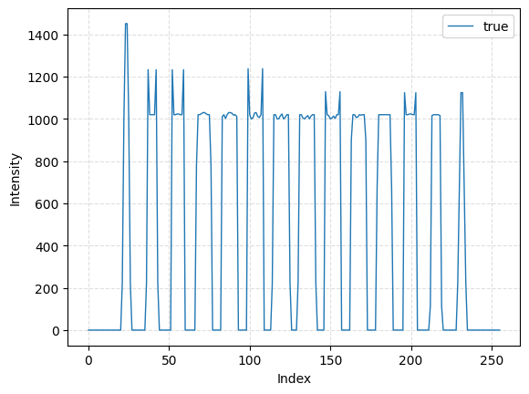
(a) The true signal.

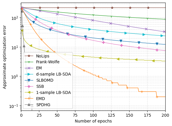
(b) Approximate optimization error versus the number of epochs.

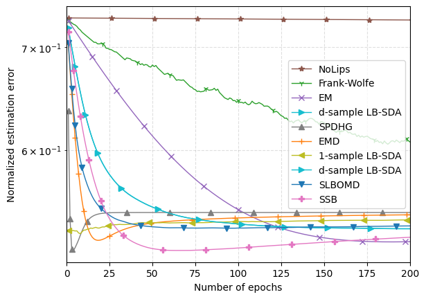
(c) Normalized estimation error versus the number of epochs.

This section presents additional numerical results in terms of the number of epochs, where one epoch refers to one full pass of the dataset. Specifically, one epoch of $B$-sample LB-SDA corresponds to $n/B$ iterations, one epoch of other stochastic methods corresponds to $n$ iterations, and one epoch of batch methods corresponds to one iteration. The number of epochs is proportional to the number of gradient evaluated by the algorithm. Note that EMD and diluted iMLE compute function values in the Armijo line search procedure, which pass through the dataset for more than once. Therefore, the numerical results in terms of the number of epochs favor these two algorithms. Since computing the function values is much faster than computing the gradients, we still present numerical results in terms of the number of epochs.

Figure 3 presents results for the experiment of Poisson inverse problem in Section 6.1, while Figure 4 presents results for the experiment of ML quantum state tomography in Section 6.2. In terms of the optimization error, $1$-sample LB-SDA outperforms other methods with clear complexity guarantees. Note that $1$-sample LB-SDA converges faster than $d$-sample LB-SDA. The reason is that after the $s$-th epoch, $1$-sample LB-SDA has performed $ns$ iterations, whereas $d$-sample LB-SDA has only performed $ns/d$ iterations. According to Corollary 7, the optimization error bound of $1$-sample LB-SDA is $\smash{\tilde{O}}(d/(ns)+\sqrt{d/(ns)})$, smaller than the $\smash{\smash{\tilde{O}}(d^{2}/(ns)+\sqrt{d/(ns)})}$ optimization error bound of $d$-sample LB-SDA. In terms of the fidelity, $1$-sample LB-SDA achieves the best performance among all methods with explicit complexity guarantees for computing the ML estimate for quantum state tomography.

Figure 4: Performances of all algorithms in Table 1, iMLE, diluted iMLE, and EMD with line search for computing the ML estimate for quantum state tomography.

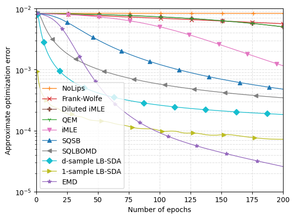
(a) Approximate optimization error versus the number of epochs.

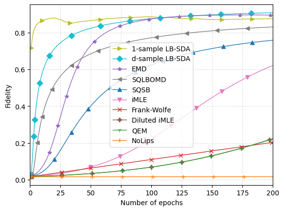
(b) Fidelity between the iterates and the $W$ state versus the number of epochs.

References

• Kelly [1956] John L. Kelly. A new interpretation of information rate. Bell Syst. tech. j., 35(4):917–926, 1956.
• Algoet and Cover [1988] Paul H. Algoet and Thomas M. Cover. Asymptotic optimality and asymptotic equipartition properties of log-optimum investment. Ann. Probab., pages 876–898, 1988.
• MacLean et al. [2011] Leonard C. MacLean, Edward O. Thorp, and William T. Ziemba. The Kelly Capital Growth Investment Criterion: Theory and Practice, volume 3. World Scientific, 2011.
• Vardi and Lee [1998] Y. Vardi and D. Lee. From image deblurring to optimal investments: Maximum likelihood solutions for positive linear inverse problems. J. R. Stat. Soc. Series B Stat. Methodol., 55(3):569–598, 1998.
• Bertero et al. [2018] Mario Bertero, Patrizia Boccacci, and Valeria Ruggiero. Inverse Imaging with Poisson Data. 2053-2563. IOP Publishing, 2018.
• Cover [1991] Thomas M. Cover. Universal portfolios. Math. Financ., 1(1):1–29, 1991.
• van Erven et al. [2020] Tim van Erven, Dirk van der Hoeven, Wojciech Kotłowski, and Wouter M. Koolen. Open problem: Fast and optimal online portfolio selection. In Proc. 33rd Annu. Conf. Learning Theory, pages 3864–3869, 2020.
• Zimmert et al. [2022] Julian Zimmert, Naman Agarwal, and Satyen Kale. Pushing the efficiency-regret Pareto frontier for online learning of portfolios and quantum states. In Proc. 35th Annu. Conf. Learning Theory, pages 182–226, 2022.
• Hradil [1997] Z. Hradil. Quantum-state estimation. Phys. Rev. A, 55, 1997.
• Yuan and Parrilo [2022] Chenyang Yuan and Pablo A. Parrilo. Maximizing products of linear forms, and the permanent of positive semidefinite matrices. Math. Program., 193(1):499–510, 2022.
• Aaronson and Arkhipov [2011] Scott Aaronson and Alex Arkhipov. The computational complexity of linear optics. In Proc. 43rd Annu. ACM Symp. Theory of Computing, pages 333–342, 2011.
• Li and Cevher [2019] Yen-Huan Li and Volkan Cevher. Convergence of the exponentiated gradient method with Armijo line search. J. Optim. Theory Appl., 181(2):588–607, 2019.
• Nesterov [2018] Yurii Nesterov. Lectures on Convex Optimization. Springer, Cham, CH, second edition, 2018.
• Lan [2020] Guanghui Lan. First-order and Stochastic Optimization Methods for Machine Learning, volume 1. Springer, 2020.
• Ben-Tal et al. [2001] Aharon Ben-Tal, Tamar Margalit, and Arkadi Nemirovski. The ordered subsets mirror descent optimization method with applications to tomography. SIAM J. Optim., 12(1):79–108, 2001.
• Ehrhardt et al. [2017] Matthias J. Ehrhardt, Pawel Markiewicz, Antonin Chambolle, Peter Richtárik, Jonathan Schott, and Carola-Bibiane Schönlieb. Faster PET reconstruction with a stochastic primal-dual hybrid gradient method. In Wavelets and Sparsity XVII, volume 10394, page 103941O. SPIE, 2017.
• Chen et al. [2023] Sitan Chen, Brice Huang, Jerry Li, Allen Liu, and Mark Sellke. When does adaptivity help for quantum state learning? arXiv preprint arXiv:2206.05265, 2023.
• Lin et al. [2021] Chien-Ming Lin, Hao-Chung Cheng, and Yen-Huan Li. Maximum-likelihood quantum state tomography by Cover’s method with non-asymptotic analysis. arXiv preprint arXiv:2110.00747, 2021.
• Lin et al. [2022] Chien-Ming Lin, Yu-Ming Hsu, and Yen-Huan Li. Maximum-likelihood quantum state tomography by soft-bayes. arXiv preprint arXiv:2012.15498, 2022.
• Tsai et al. [2022] Chung-En Tsai, Hao-Chung Cheng, and Yen-Huan Li. Faster stochastic first-order method for maximum-likelihood quantum state tomography. arXiv preprint arXiv:2211.12880, 2022.
• Hanzely and Richtárik [2021] Filip Hanzely and Peter Richtárik. Fastest rates for stochastic mirror descent methods. Comput. Optim. Appl., 79(3):717–766, 2021.
• D’Orazio et al. [2021] Ryan D’Orazio, Nicolas Loizou, Issam Laradji, and Ioannis Mitliagkas. Stochastic mirror descent: Convergence analysis and adaptive variants via the mirror stochastic polyak stepsize. arXiv preprint arXiv:2110.15412, 2021.
• Chambolle et al. [2018] Antonin Chambolle, Matthias J. Ehrhardt, Peter Richtárik, and Carola-Bibiane Schönlieb. Stochastic primal-dual hybrid gradient algorithm with arbitrary sampling and imaging applications. SIAM J. Optim., 28(4):2783–2808, 2018.
• Alacaoglu et al. [2022] Ahmet Alacaoglu, Olivier Fercoq, and Volkan Cevher. On the convergence of stochastic primal-dual hybrid gradient. SIAM J. Optim., 32(2):1288–1318, 2022.
• He et al. [2020] Niao He, Zaid Harchaoui, Yichen Wang, and Le Song. Point process estimation with mirror prox algorithms. Appl. Math. Optim., 82(3):919–947, 2020.
• Fercoq and Bianchi [2019] Olivier Fercoq and Pascal Bianchi. A coordinate-descent primal-dual algorithm with large step size and possibly nonseparable functions. SIAM J. Optim., 29(1):100–134, 2019.
• Dekel et al. [2012] Ofer Dekel, Ran Gilad-Bachrach, Ohad Shamir, and Lin Xiao. Optimal distributed online prediction using mini-batches. J. Mach. Learn. Res., 13(1), 2012.
• Williams et al. [2023] Virginia Vassilevska Williams, Yinzhan Xu, Zixuan Xu, and Renfei Zhou. New bounds for matrix multiplication: from alpha to omega. arXiv preprint arXiv:2307.07970, 2023.
• Dongarra et al. [1990] J. J. Dongarra, Jeremy Du Croz, Sven Hammarling, and I. S. Duff. A set of level 3 basic linear algebra subprograms. ACM Trans. Math. Softw., 16(1):1–17, 1990.
• Tsai et al. [2023a] Chung-En Tsai, Ying-Ting Lin, and Yen-Huan Li. Data-dependent bounds for online portfolio selection without lipschitzness and smoothness. arXiv preprint arXiv:2305.13946, 2023a.
• Cesa-Bianchi et al. [2004] N. Cesa-Bianchi, A. Conconi, and C. Gentile. On the generalization ability of on-line learning algorithms. IEEE Trans. Inf. Theory, 50(9):2050–2057, 2004.
• Cutkosky [2019] Ashok Cutkosky. Anytime online-to-batch, optimism and acceleration. In Proc. 36th Int. Conf. Machine Learning, volume 97, pages 1446–1454, 2019.
• Bauschke et al. [2017] Heinz H. Bauschke, Jérôme Bolte, and Marc Teboulle. A descent lemma beyond Lipschitz gradient continuity: first-order methods revisited and applications. Math. Oper. Res., 42(2):330–348, 2017.
• Zhao and Freund [2023] Renbo Zhao and Robert M. Freund. Analysis of the Frank–Wolfe method for convex composite optimization involving a logarithmically-homogeneous barrier. Math. Program., 199(1):123–163, 2023.
• Shepp and Vardi [1982] L. A. Shepp and Y. Vardi. Maximum likelihood reconstruction for emission tomography. IEEE Trans. Med. Imaging, 1(2):113–122, 1982.
• Cover [1984] Thomas M. Cover. An algorithm for maximizing expected log investment return. IEEE Trans. Inf. Theory, 30(2):369–373, 1984.
• Tran-Dinh et al. [2015] Quoc Tran-Dinh, Anastasios Kyrillidis, and Volkan Cevher. Composite self-concordant minimization. J. Mach. Learn. Res., 16(12):371–416, 2015.
• Dvurechensky et al. [2023] Pavel Dvurechensky, Kamil Safin, Shimrit Shtern, and Mathias Staudigl. Generalized self-concordant analysis of Frank–Wolfe algorithms. Math. Program., 198(1):255–323, 2023.
• Carderera et al. [2021] Alejandro Carderera, Mathieu Besançon, and Sebastian Pokutta. Simple steps are all you need: Frank-Wolfe and generalized self-concordant functions. In Adv. Neural Information Processing Systems, volume 34, pages 5390–5401, 2021.
• Liu et al. [2022] Deyi Liu, Volkan Cevher, and Quoc Tran-Dinh. A Newton Frank–Wolfe method for constrained self-concordant minimization. J. Glob. Optim., 83(2):273–299, 2022.
• Řeháček et al. [2007] Jaroslav Řeháček, Zdeněk Hradil, E. Knill, and A. I. Lvovsky. Diluted maximum-likelihood algorithm for quantum tomography. Phys. Rev. A, 75(4):042108, 2007.
• Gonçalves et al. [2014] Doglas S. Gonçalves, Márcia A. Gomes-Ruggiero, and Carlile Lavor. Global convergence of diluted iterations in maximum-likelihood quantum tomography. Quantum Info. Comput., 14(11–12):966–980, 2014.
• Hudson and Larkin [1994] H. M. Hudson and R. S. Larkin. Accelerated image reconstruction using ordered subsets of projection data. IEEE Trans. Med. Imaging, 13(4):601–609, 1994.
• Lvovsky [2004] A. I. Lvovsky. Iterative maximum-likelihood reconstruction in quantum homodyne tomography. J. Opt. B: Quantum and Semiclass. Opt., 6(6):S556, 2004.
• Häffner et al. [2005] H. Häffner, W. Hänsel, C. F. Roos, J. Benhelm, D. Chek-al kar, M. Chwalla, T. Körber, U. D. Rapol, M. Riebe, P. O. Schmidt, C. Becher, O. Gühne, W. Dür, and R. Blatt. Scalable multiparticle entanglement of trapped ions. Nature, 438(7068):643–646, 2005.
• Palmieri et al. [2020] Adriano Macarone Palmieri, Egor Kovlakov, Federico Bianchi, Dmitry Yudin, Stanislav Straupe, Jacob D. Biamonte, and Sergei Kulik. Experimental neural network enhanced quantum tomography. npj Quantum Inf., 6(1):20, 2020.
• Brown et al. [2023] M. O. Brown, S. R. Muleady, W. J. Dworschack, R. J. Lewis-Swan, A. M. Rey, O. Romero-Isart, and C. A. Regal. Time-of-flight quantum tomography of an atom in an optical tweezer. Nat. Phys., 19(4):569–573, 2023.
• Meiburg [2022] Alexander Meiburg. Inapproximability of positive semidefinite permanents and quantum state tomography. In IEEE 63rd Annu. Symp. Foundations of Computer Science, pages 58–68, 2022.
• Srebro et al. [2010] Nathan Srebro, Karthik Sridharan, and Ambuj Tewari. Smoothness, low-noise and fast rates. In Adv. Neural Information Processing Systems, volume 23, 2010.
• Orabona [2023] Francesco Orabona. A modern introduction to online learning. arXiv preprint arXiv:1912.13213v6, 2023.
• Demmel et al. [2007] James Demmel, Ioana Dumitriu, and Olga Holtz. Fast linear algebra is stable. Numer. Math., 108(1):59–91, 2007.
• Bezanson et al. [2017] Jeff Bezanson, Alan Edelman, Stefan Karpinski, and Viral B Shah. Julia: A fresh approach to numerical computing. SIAM Review, 59(1):65–98, 2017.
• Shepp and Logan [1974] Lawrence A Shepp and Benjamin F Logan. The Fourier reconstruction of a head section. IEEE Trans. Nuc. Sci, 21(3):21–43, 1974.
• Raginsky et al. [2010] Maxim Raginsky, Rebecca M. Willett, Zachary T. Harmany, and Roummel F. Marcia. Compressed sensing performance bounds under Poisson noise. IEEE Trans. Signal Process., 58(8):3990–4002, 2010.
• Li [2020] Yen-Huan Li. Online positron emission tomography by online portfolio selection. In IEEE Int. Conf. Acoustics, Speech and Signal Processing, pages 1110–1114, 2020.
• Li et al. [2018] Yen-Huan Li, Carlos A Riofrío, and Volkan Cevher. A general convergence result for mirror descent with Armijo line search. arXiv preprint arXiv:1805.12232, 2018.
• Shang et al. [2017] Jiangwei Shang, Zhengyun Zhang, and Hui Khoon Ng. Superfast maximum-likelihood reconstruction for quantum tomography. Phys. Rev. A, 95:062336, 2017.
• Ahmed et al. [2021] Shahnawaz Ahmed, Carlos Sánchez Muñoz, Franco Nori, and Anton Frisk Kockum. Quantum state tomography with conditional generative adversarial networks. Phys. Rev. Lett., 127:140502, 2021.
• Bottou and Bousquet [2007] Léon Bottou and Olivier Bousquet. The tradeoffs of large scale learning. In Adv. Neural Information Processing Systems, volume 20, 2007.
• Nesterov and Nemirovskii [1994] Yurii Nesterov and Arkadii Nemirovskii. Interior-Point Polynomial Algorithms in Convex Programming. SIAM, Philadelphia, PA, 1994.
• Lu et al. [2018] Haihao Lu, Robert M. Freund, and Yurii Nesterov. Relatively smooth convex optimization by first-order methods, and applications. SIAM J. Optim., 28(1):333–354, 2018.
• Tsai et al. [2023b] Chung-En Tsai, Hao-Chung Cheng, and Yen-Huan Li. Online self-concordant and relatively smooth minimization, with applications to online portfolio selection and learning quantum states. In Proc. 34th Int. Conf. Algorithmic Learning Theory, pages 1481–1483, 2023b. arXiv:2210.00997.
• Hazan [2016] Elad Hazan. Introduction to Online Convex Optimization. Found. Trends Opt., 2(3–4):157–325, 2016.
• Boyd and Vandenberghe [2004] Stephen P. Boyd and Lieven Vandenberghe. Convex Optimization. Cambridge university press, 2004.
• Hiai and Petz [2014] Fumio Hiai and Dénes Petz. Introduction to Matrix Analysis and Applications. Springer, Cham, 2014.
• Luo et al. [2018] Haipeng Luo, Chen-Yu Wei, and Kai Zheng. Efficient online portfolio with logarithmic regret. In Adv. Neural Information Processing Systems, volume 31, 2018.