IPVNet: Learning Implicit Point-Voxel Features for Open-Surface 3D Reconstruction

Abstract

Reconstruction of 3D open surfaces (e.g., non-watertight meshes) is an underexplored area of computer vision. Recent learning-based implicit techniques have removed previous barriers by enabling reconstruction in arbitrary resolutions. Yet, such approaches often rely on distinguishing between the inside and outside of a surface in order to extract a zero level set when reconstructing the target. In the case of open surfaces, this distinction often leads to artifacts such as the artificial closing of surface gaps. However, real-world data may contain intricate details defined by salient surface gaps. Implicit functions that regress an unsigned distance field have shown promise in reconstructing such open surfaces. Nonetheless, current unsigned implicit methods rely on a discretized representation of the raw data. This not only bounds the learning process to the representation’s resolution, but it also introduces outliers in the reconstruction. To enable accurate reconstruction of open surfaces without introducing outliers, we propose a learning-based implicit point-voxel model (IPVNet). IPVNet predicts the unsigned distance between a surface and a query point in 3D space by leveraging both raw point cloud data and its discretized voxel counterpart. Experiments on synthetic and real-world public datasets demonstrates that IPVNet outperforms the state of the art while producing far fewer outliers in the resulting reconstruction.

1 Introduction

(a)

(b)

Fig. 1: An outside view of a dense 3D reconstructed scene from the Gibson Environment [1] dataset using (a) the state of the art [2], and (b) our proposed approach. Note that our method produces significantly less outliers.

3D computer vision for generating (e.g., [3, 4]) and reconstructing (e.g., [5, 6]) point clouds has gained momentum due to applications such as robotics, autonomous driving, and virtual reality. Capturing detailed point cloud data from the real world is a difficult and expensive task. Moreover, due to the limitations of 3D sensor technologies (e.g., LiDAR, RGBD, etc.), data can be sparse (i.e., missing details) and incomplete (i.e., noisy with holes and outliers). The 3D reconstruction of missing parts and reintroduction of details is not a trivial task. Researchers have looked into a myriad of ways to complete 3D data. Learning-based implicit functions have become popular among 3D reconstruction techniques due to their demonstrated superiority in capturing details and the ability to generate data in arbitrary resolutions.

Implicit functions operate by first converting raw data into an occupancy grid and then learning a voxel occupancy or a distance field that classifies a query point as either inside or outside of the surface. In low resolutions, occupancy grids lose information during voxelization since multiple points within the boundary of a grid are merged together. To preserve fine details in the input data, a high-resolution representation is required. However, the computational costs and memory requirements increase cubically with voxel resolution. For example, Chibane et al. [2] require 8.86 GB of memory to train with a single input (batch size 1) at a resolution of $256^{3}$. This large memory footprint makes it impractical to scale beyond the aforesaid resolution.

Instead of relying on the voxels, researchers have also tried to use raw point clouds with a learned signed distance field (SDF) on the surface. Nevertheless, implicit functions that learn an SDF via extraction of a zero level set must distinguish between the inside/outside of the surface. As a result, the reconstruction is produced as a closed surface even if the target shape includes surface gaps. However, real-world data may consist of salient open surfaces. Closing the surface of such data often leads to the introduction of outliers and lost details.

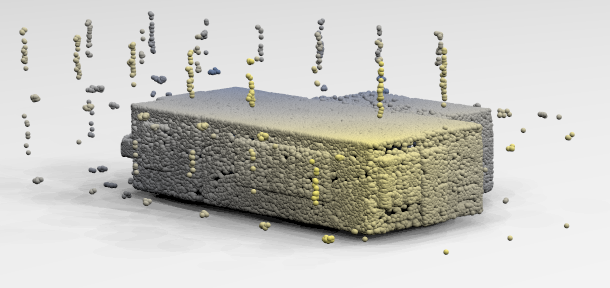
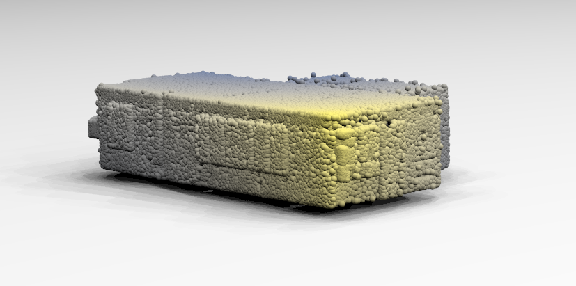
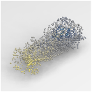
To reconstruct accurate geometry without introducing outliers, we propose IPVNet, an implicit model that learns an unsigned distance field (UDF) by jointly accumulating features from raw point clouds and voxel grids to reconstruct open surfaces. As shown in Fig. 1, our approach produces significantly less outliers compared to the state of art [2]. Note that by reconstructing a surface, we refer to the construction of dense point clouds that lie on the surface, which is a key part of the reconstruction process. Although one could extract and render the surface mesh from such point clouds, we present our results in the form of raw point clouds. For completeness, we record additional results as rendered meshes in our experimental evaluation.

The technique of learning features from both point clouds and voxels has been shown to achieve superior performance in classification and segmentation, detection, and generation. However, to the best of our knowledge, our work is the first approach to combine point-voxel features to learn a UDF for open-surface reconstruction. Such improved features allow our model to reconstruct richer detail even with low-resolution voxel grids. Moreover, the involvement of raw point features allows us to use a more sophisticated inference module that produces significantly fewer outliers in the reconstructed output. Our key contributions are summarized as follows.

• We introduce IPVNet, a novel approach for implicitly learning from raw point cloud and voxel features to 3D reconstruct complex open surfaces.

• We develop an inference module that extracts a zero level set from a UDF and drastically lowers the amount of outliers in the reconstruction.

• We show that IPVNet outperforms the state of the art on both synthetic and real-world public datasets, and we provide an ablation analysis to understand the importance of point-voxel fusion.

To reproduce and improve upon our results, the project source code is publicly available to the research community [7].

The remainder of this paper is organized as follows. We provide an overview of related research in Sec. 2. In Sec. 3, a concise summary of implicit functions is provided. The details of IPVNet are presented in Sec. 4, and the experimental evaluation and results are described in Sec. 5. We discuss limitations and future directions of our work in Sec. 7 and a conclusion is given in Sec. 8.

2 Related work

3D reconstruction is a well researched area with a number of different approaches and algorithms. In this section, we review and compare our work with learning-based implicit approaches. For a more comprehensive review, we refer the reader to a contemporary survey on 3D reconstruction [8].

2.1 Implicit function learning

Instead of explicitly predicting a surface, implicit feature learning methods try to either predict if a particular point in 3D space is inside or outside of a target surface (occupancy), or determine how far the point is from the target surface (distance). To reconstruct 3D data in arbitrary resolutions and learn a continuous 3D mapping, Mescheder et al. [9] presented a network that predicts voxel occupancy. Peng et al. [10] improved the occupancy network by incorporating 2D and 3D convolutions. An encoder-decoder architecture was used by Chen et al. [11] to learn voxel occupancy. Michalkiewicz et al. [12] estimated an oriented level set to extract a 3D surface. Littwin and Wolf [13] used encoded feature vectors as the network weights to predict voxel occupancy. Park et al. [14] introduced DeepSDF, an encoder-decoder architecture that predicts a signed distance to the surface instead of voxel occupancy. Genova et al. [15] divided an object’s surface into a set of shape elements and utilized an encoder-decoder to learn occupancy. Sitzmann et al. [16] introduced SIREN to implicitly learn complex signals for various downstream tasks including 3D shape representations via a signed distance function.

Fig. 2: A 2D representation of a closed (top row) and an open (bottom row) surface reconstruction via occupancy, signed distance field (SDF), and unsigned distance field (UDF). Note that the occupancy and SDF reconstructions of the open surface closes the gap by producing an artifact while a UDF can preserve the surface opening. The color intensity represents the distance from the surface where blue represents a positive value, and red represents a zero (occupancy) or negative value (SDF).

Bhatnagar et al. [17] combined implicit functions with parametric modeling to jointly reconstruct body shape under clothing by predicting occupancy. To retain richer details in the reconstruction, Chibane et al. [18] used 3D feature tensors to predict voxel occupancy. Rather than transforming point clouds into a occupancy grid, Atzmon and Lipman made use of raw point clouds to learn and predict an SDF to the target surface [19], and later incorporated derivatives in a regression loss to further improve the reconstruction accuracy [20]. Gropp et al. [21] used geometric regularization to learn directly from raw point clouds. To make the reconstruction process more scalable, Mi et al. [22] introduced SSRNet to construct local geometry-aware features for octree vertices. By leveraging gradient-based meta-learning algorithms, Sitzmann et al. [23] developed MetaSDF to improve the generalization ability of implicit learning.

With a similar aim of improving generalization, Tretschk et al. [24] created a patch-based representation to learn an SDF. A local implicit grid to learn an SDF and reconstruct 3D data was used by Jiang et al. [25]. Liu et al. [26] implemented deep implicit least squares to regress an SDF for 3D reconstruction. Deep implicit fusion to estimate an SDF for online 3D reconstruction was presented by Huang et al. [27]. Duggal et al. [28] used signed distance regression via neural implicit modeling for 3D vehicle reconstruction from partial/noisy data. Sign agnostic learning to estimate a signed implicit field of a local surface for 3D reconstruction was proposed by Zhao et al. [29].

All of the aforementioned works either predict a voxel occupancy or a signed distance value for a given query point, which is inadequate to reconstruct open surfaces. To alleviate this inadequacy, Chibane et al. [2] predicted a UDF from an input voxel occupancy. A similar technique to learn a UDF for single-view garment reconstruction was used by Zhao et al. [30]. Venkatesh et al. [31] proposed a closest surface point representation to reconstruct both open and closed surfaces. A new NULL sign combined with conventional in and out labels to reconstruct a non-watertight arbitrary topology was proposed by Chen et al. [32]. Ye et al. [33] leveraged the relationship between every two points, instead of points and surfaces, to improve the reconstruction quality of non-watertight 3D shapes. The aforementioned works only utilize the discretized voxel representation while we make use of raw point clouds jointly with voxel occupancy. This enables us to accumulate improved features and reconstruct finer details with less outliers.

2.2 Learning from points and voxels

Due to the convenience of using volumetric convolutions, many works have explored voxel-based representations (e.g., [34, 35, 36]). However, voxel grids grow cubically with resolution and their memory intensiveness imposes an upper bound to the highest resolution possible. Point clouds are memory efficient, yet it is non-trivial to extract features from them due to their sparsity and permutation invariant nature. Recently, researchers started combining these two representations to get the best out of them both.

Liu et al. [37] introduced PVCNN to perform classification and segmentation by extracting features from both point clouds and voxel grids via voxelization and de-voxelization. Fusion between voxel and point features for 3D classification was used by Li et al. [38]. Shi et al. [39] gathered multi-scale voxel features and combined them with point cloud keypoint features for object detection. They further improved their results by incorporating local vector pooling [40]. Point-voxel fusion to detect 3D objects was used by Cui et al. [41] and Tang et al. [42] learned a 3D model via sparse point-voxel convolution.

Noh et al. [43] accumulated point-voxel features in a single representation for 3D object detection. PVT, a transformer-based architecture that learns from point-voxel features for point cloud segmentation was introduced by Zhang et al. [44]. Wei et al. [45] used point-voxel correlation for scene flow estimation and Li et al. [46] utilized point-voxel convolution for 3D object detection. Xu et al. [47] introduced RPVNet for point cloud segmentation via point-voxel fusion. Cherenkova et al. [48] utilized point-voxel deconvolution for point cloud encoding/decoding. In contrast to the preceding works, we use a point-voxel representation to learn an implicit function for open-surface reconstruction. To restore lost details during voxelization, we propose a novel aggregation strategy that accumulates features from both point clouds and voxel grids.

3 Background

Implicit functions rely on one of three output choices for surface reconstruction. Concretely, given a latent representation $z\in\mathcal{Z}$ of a point cloud object $x\in\mathcal{X}\subset\mathbb{R}^{N\times 3}$ and a random query point $p\in\mathbb{R}^{3}$, an implicit function $f$ aims to predict the following.

1. Occupancy, i.e., if $p$ lies inside or outside the object,

   $$f(z,p):\mathcal{Z}\times\mathbb{R}^{3}\rightarrow[0,1].$$ (1)

2. Signed distance, i.e., the distance from $p$ to the inside or outside surface of the object,

   $$f(z,p):\mathcal{Z}\times\mathbb{R}^{3}\rightarrow\mathbb{R}.$$ (2)

3. Unsigned distance, i.e., the absolute distance from $p$ to any surface on the object,

   $$f(z,p):\mathcal{Z}\times\mathbb{R}^{3}\rightarrow\mathbb{R}_{+}.$$ (3)

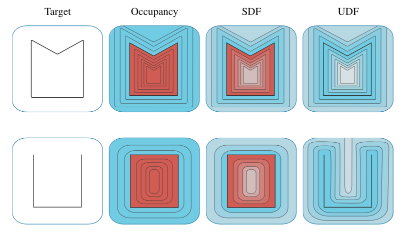
In (1) - (3), $\mathcal{X}$ denotes the input space, $\mathcal{Z}$ is the latent space, and $N\in\mathbb{N}$ is the density/resolution of the point cloud. After learning the implicit function $f$, it may be queried multiple times to find the decision boundary (occupancy) or the zero level set (signed and unsigned distance) thus implicitly reconstructing the surface of the desired object. Fig. 2 provides an overview of open/closed surface reconstruction via different implicit techniques in 2D.

4 Implicit learning with point-voxel features

Fig. 3: Given a sparse point cloud $x\in\mathcal{X}$ of an object, we use a novel encoding scheme to extract and aggregate point-voxel features from both the raw point cloud $(x)$ and the voxel occupancy $(v)$. From the accumulated features, a decoder module regresses the unsigned distance $UD(p,S)$ from query point $p$ to the surface $S$. By querying the decoder multiple times, the inference sub-module can reconstruct the surface of any target shape.

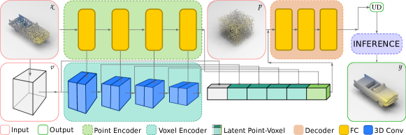
An overview of our network is presented in Fig. 3. We have chosen unsigned distances as the output representation of IPVNet due to their precedence in representing different surfaces. Given a sparse point cloud $x\in\mathcal{X}\subset\mathbb{R}^{N\times 3}$ of an object, we use a novel encoding scheme to extract and aggregate point-voxel features from both the raw point cloud $(x)$ and the voxel occupancy $(v)$. From the accumulated features, a decoder module regresses the unsigned distance $UD(p,S)$ via any query point $p$ to the surface $S$. In the following subsections we describe the elements of our approach.

4.1 Point-voxel features

To extract a set of multi-level features from a point cloud $x$, we define a neural function

$$\Theta(x):=(z_{x}^{1},\ldots,z_{x}^{j})\>|\>\Theta\colon\mathbb{R}^{3}\rightarrow\mathcal{Z},$$ (4)

where $z_{x}\in\mathcal{Z}\subset\mathbb{R}$ corresponds to the extracted feature vector from the raw point cloud $x$, and $j$ is the total number of layers in $\Theta$. During the early stages (i.e., when $j=1$) the encoder is more focused on local details, whereas at the later stages the focus is shifted towards the global structure. ReLu [49] nonlinearity is used for all layers except the output layer of the point encoder.

Instead of limiting the encoded features to a single dimensional vector, a voxel representation allows for the construction of a multi-dimensional latent matrix. However, such an encoding scheme requires the input point cloud $x$ to be discretized into a voxel grid $v$, i.e., $x\approx v\colon\mathbb{R}^{N\times 3}\rightarrow\mathbb{R}^{M\times M\times M}$ where $M\in\mathbb{N}$ is the grid resolution. Due to the discretization process, voxel grids lose information since multiple points may lie within the same voxel. To reintroduce lost details, we combine voxel features with point features $z_{x}$. Although, a different fusion strategy can be applied to combine these features, we empirically found that a simple concatenation strategy works best.

Let $\Phi\colon\mathbb{R}^{M\times M\times M}\rightarrow\mathcal{Z}^{M\times M\times M}$ be a neural function that encodes the combined point-voxel features into a set of multi-dimensional feature grids $z_{xv}$ of monotonically decreasing dimension. Then,

$$\Phi(v\odot\Theta(x)):=(z_{xv}^{k\times k\times k},\ldots,z_{xv}^{l\times l\times l}),$$ (5)

where $k,l\in\mathbb{N}$ represents the dimensional upper and lower bound of the feature grid $(M>k\gg l>1)$. The subscript ${xv}$ denotes the dependency on both points and voxels. Similar to its point counterpart, the voxel encoder is more directed towards local details at the early stages. However, as the dimensionality is reduced and the receptive field grows larger, the aim shifts to the global structure. ReLu is utilized to ensure nonlinearity and batch normalization [50] provides stability while training. The latent point ($z_{x}^{j}$) from the point encoder, along with multi-dimensional features ($z_{xv}$) from the point-voxel encoder and the discretized voxel grid ($v$), are then used to construct the latent point-voxel:

$$z=\{z_{x}^{j},\Phi(v\odot\Theta(x)),v\}.$$ (6)

4.2 Implicit decoding

Given a query point $p\in\mathbb{R}^{3}$, a set of deep features $F_{p}$ is sampled from the latent point-voxel features $z$ via a sampling function $\Omega$ [51]. Specifically,

$$\Omega(z,p):=(F_{p}^{1}\times\dots\times F_{p}^{n}),$$ (7)

where $n=\lvert z\rvert$. We extract features from a neighborhood of distance $d\in\mathbb{R}$ along the Cartesian axes centered at $p$ to obtain rich features. More formally,

$$p:=\{p+q\cdot c_{i}\cdot d\}\in\mathbb{R}^{3}\;|\;q\in\{1,0,-1\},i\in\{1,2,3\},$$ (8)

where $c_{i}\in\mathbb{R}^{3}$ is the $ith$ Cartesian axis unit vector. We define a neural function $\Psi$ that regresses the unsigned distance to the surface $S$ of $x$ from the deep features ($F_{p}$). Concretely,

$$\Psi(F_{p}^{1},\dots,F_{p}^{n})\approxeq UD(p,S)\;|\;\Psi\colon\mathcal{Z}\rightarrow\mathbb{R}_{+},$$ (9)

where $UD(\cdot)$ is a function that returns the unsigned distance from $p$ to the ground-truth surface $S$ for any $p\in\mathbb{R}^{3}$. Hence, the implicit decoder to regress the unsigned distance at a given query point $p$ is defined as

$$f_{x}(z,p):=(\Omega\circ\Psi)(p)\;|\;f_{x}\colon\mathcal{Z}\times\mathbb{R}^{3}\rightarrow\mathbb{R}_{+}.$$ (10)

4.3 Training

IPVNet requires a pair $\{X_{i},S_{i}\}^{T}_{i=1}$ associated with input $X_{i}$ and corresponding ground-truth surface $S_{i}$ for implicit learning. Parameterized by the neural parameter $w$, the point-encoder, voxel-encoder, and decoder are jointly trained with a mini-batch loss,

$$\mathcal{L}_{\mathcal{B}}:=\Sigma_{x\in B}\Sigma_{p\in\mathcal{P}}|\min(f_{x}^{w}(p),\delta)-\min(UD(p,S_{x}),\delta)|,$$ (11)

where $\mathcal{B}$ is a mini-batch of input and $\mathcal{P}\in\mathbb{R}^{3}$ is a set of query points within distance $\delta$ of $S_{i}$. We use a clamped distance $0<\delta<10$ (cm) to improve the capacity of the model to represent the vicinity of the surface accurately.

4.4 Surface inference

We use an iterative strategy to extract surface points from $f_{x}$. More specifically, given a perfect approximator $f_{x}(p)$ of the true unsigned distance $UD(p,S_{i})$, the projection of $p$ onto the surface $S_{i}$ can be obtained by

$$q:=p-f_{x}(p)\cdot\nabla_{p}f_{x}(p),\quad q\in S_{i}\subset\mathbb{R}^{d},\forall p\in\mathbb{R}^{d}/C.$$ (12)

In (12), $C$ is the cut locus [52], i.e., a set of points that are equidistant to at least two surface points. The negative gradient indicates the direction of the fastest decrease in distance. In addition, we can move a distance of $f_{x}(p)$ to reach $q$ if the norm of the gradient is one. By projecting a point multiple times via (12), the inaccuracies due to $f_{x}(p)$ being an imperfect approximator can be reduced. Furthermore, filtering the projected points to a maximum distance threshold ($max\_thresh$) and re-projecting them onto the surface after displacement by $d\sim\mathcal{N}(0,\delta/3)$ can ensure higher point density within a maximum distance ($\delta$).

Instead of uniformly sampling query points within the bounding box of $S_{i}$, we use the input points $X_{i}\in\mathbb{R}^{3}$ as guidance for the query points. In particular, we apply a random uniform jitter $\mathcal{J}_{a}^{b}\in\mathbb{R}^{3}$ within bounds $a$ and $b$ to displace the input points $X_{i}$. Due to the inclusion of point features in learning, this procedure allows our model to infer more accurate surface points while restricting the number of outliers. Note that without the use of point features, this perturbation of the input points fails to restrict the number of outliers (see Sec. 6). The details of the inference procedure are provided in Alg. 1.

Algorithm 1 Surface Point Inference

1:procedure Inference($\mathcal{X}$)

2:     $\mathcal{J}\leftarrow m$ points from $\textit{U}(a,b)$

3:     $\mathcal{P}_{init}\leftarrow\{x+j\},\forall x\in\mathcal{X},\forall j\in\mathcal{J}$

4:     for $i=1$ to $num\_projections$ do

5:         $p\leftarrow p-f_{x}(p)\cdot\frac{\nabla_{p}f_{x}(p)}{||\nabla_{p}f_{x}(p)||},\forall p\in\mathcal{P}_{init}$

6:     end for

7:     $\mathcal{P}_{filtered}\leftarrow\{p\in\mathcal{P}_{init}\,|\,f_{x}(p)<max\_thresh\}$

8:     $\mathcal{P}_{filtered}$: draw $out\_res$ number of points with replacement

9:     $\mathcal{P}_{filtered}\leftarrow\{p+d\}\,|\,p\in\mathcal{P}_{filtered},d\sim\mathcal{N}(0,\delta/3)$

10:     for $i=1$ to $num\_projections$ do

11:         $p\leftarrow p-f_{x}(p)\cdot\frac{\nabla_{p}f_{x}(p)}{||\nabla_{p}f_{x}(p)||},\forall p\in\mathcal{P}_{filtered}$

12:     end for

13:     return $\{p\in\mathcal{P}_{filtered}\,|\,f_{x}(p)<max\_dist\}$

14:end procedure

4.5 Implementation details

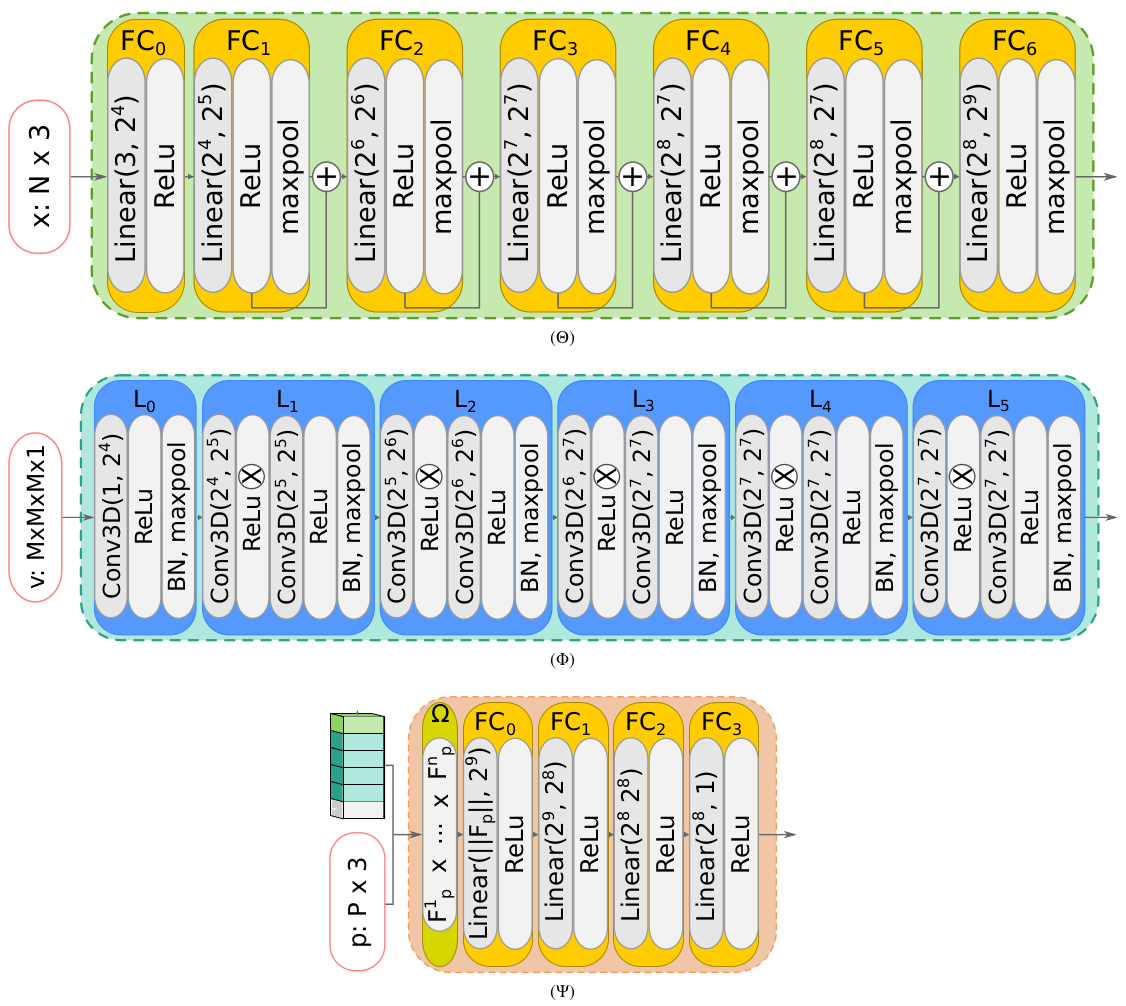
IPVNet was implemented using PyTorch. To extract point cloud and voxel features, we utilize multilayer perceptrons (MLPs) and 3D convolutional neural networks (CNNs), respectively. Specifically, we employ a 7-layer fully-connected MLP as the point encoder and 6-layer CNN blocks as the voxel encoder. Point features are obtained from each of the hidden layers of the point encoder and are combined with voxel features derived from the initial layer of each convolution block. We use max pooling with the fully-connected layers to make them permutation invariant.

Fig. 4 shows the details of the different neural modules of IPVNet. To train the model, we used a learning rate of $10^{-6}$ and the Adam [53] optimizer. With a voxel resolution of $256^{3}$ and a batch size of 4, it takes around 3.2 seconds to perform a forward pass using 4 Nvidia GeForce GTX 1080 Ti GPUs. To infer a single target surface with a dense point cloud consisting of 1 million points, IPVNet takes approximately 120 seconds.

Fig. 4: A visual depiction of the different neural architectures of IPVNet. $\bigoplus$ in ($\Theta$) represents concatenation, and $\bigotimes$ in ($\Phi$) indicates the fusion of point features with voxel features.

5 Experiments

In this section, we validate the performance of IPVNet on the task of 3D object and scene reconstruction from sparse point clouds.

5.1 Baselines and metrics

To compare the reconstruction quality of IPVNet, we utilized the open-source implementations of NDF [2] and GIFS [33] as baseline methods. For an unbiased comparison, we trained an NDF following the directions from [2] on our train-test split until a minimum validation accuracy was achieved. To quantitatively measure the reconstruction quality, we used the chamfer-$L_{2}$ distance (CD) to measure the accuracy and completeness of the surface. The CD is defined as

$$d_{CD}(Y,Y_{gt})=\sum_{i\in Y}\min_{j\in Y_{gt}}{||i-j||}^{2}+\sum_{j\in Y_{gt}}\min_{i\in Y}{||j-i||}^{2},$$ (13)

where $Y_{gt}\in\mathbb{R}^{\mathcal{O}\times 3}$ is the ground-truth point cloud, $Y\in\mathbb{R}^{\mathcal{O}\times 3}$ is the reconstructed point cloud, and $\mathcal{O}\in\mathbb{N}$ is the point density of the ground truth and the output. In addition, precision and recall are two metrics that have been extensively used to evaluate 3D reconstruction results. Precision quantifies the accuracy while recall assesses the completeness of the reconstruction. For the ground truth $Y_{gt}$ and reconstructed point cloud $Y$, the precision of an outcome at a threshold $d$ can be calculated as

$$P(d)=\sum_{i\in Y}[\min_{j\in Y_{gt}}||i-j||<d].$$

Similarly, the recall for a given $d$ is computed as

$$R(d)=\sum_{j\in Y_{gt}}[\min_{i\in Y}||j-i||<d].$$

The F-score, proposed in [54] as a comprehensive evaluation, combines precision and recall to quantify the overall reconstruction quality. Formally, the F-score at $d$ is given by

$$F(d)=\frac{2\cdot P(d)\cdot R(d)}{P(d)+R(d)}.$$

An F-score of 1 indicates perfect reconstruction.

5.2 Object reconstruction

Due to the abundance of surface openings, we chose the “Cars” subset of the ShapeNet [55] dataset for our object reconstruction experiment. We used a random split of $70\%$-$10\%$-$20\%$ for training, validation, and testing, respectively. To prepare the ground truth and input points we followed the data preparation procedure outlined in [2]. Additionally, we fixed the output point density to $\mathcal{O}=1$ million to extract a smooth mesh from the point cloud using a naive algorithm (e.g., [56]).

(a) Input

(b) NDF

(c) IPVNet

(d) IPVNet (Inner View)

(e) GT

(f)

(g)

(h)

(i)

(j)

(k)

(l)

(m)

(n)

(o)

Fig. 5: Object reconstruction using NDF [2], IPVNet, and the ground truth (GT) from the ShapeNet Cars [55] test set. IPVNet performs better on reconstructing thin structures and preserving small gaps (inset images).

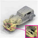
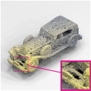
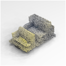
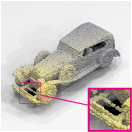
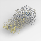
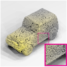
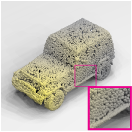
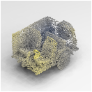
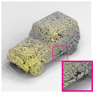
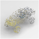
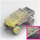
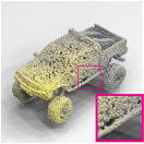
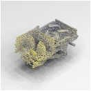
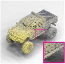
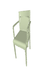
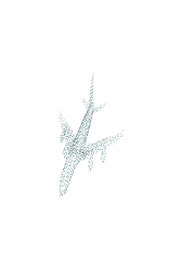
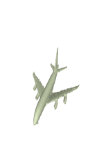
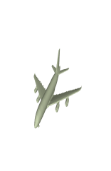
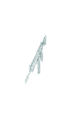
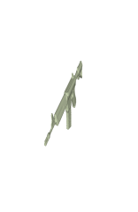
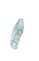
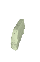
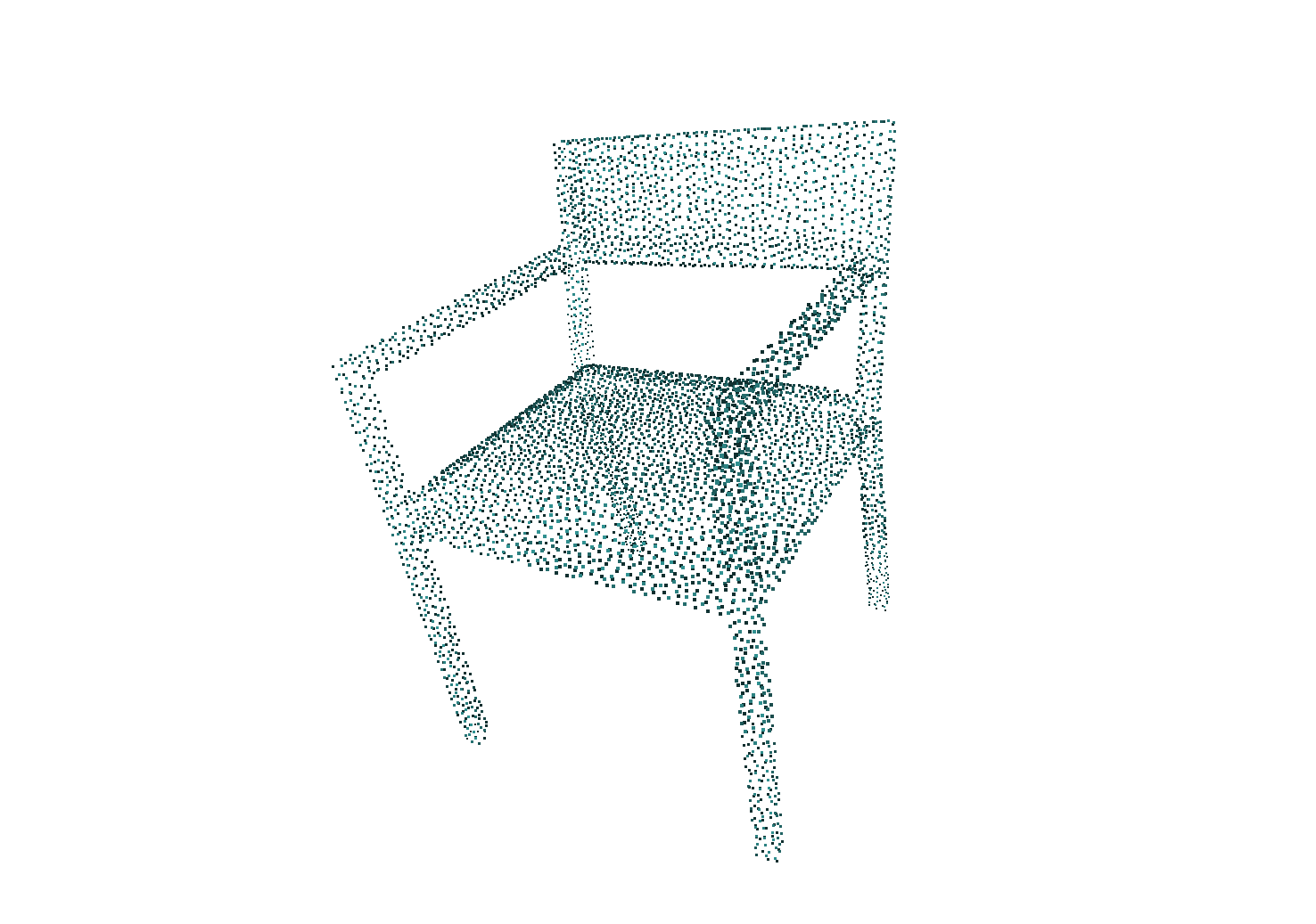
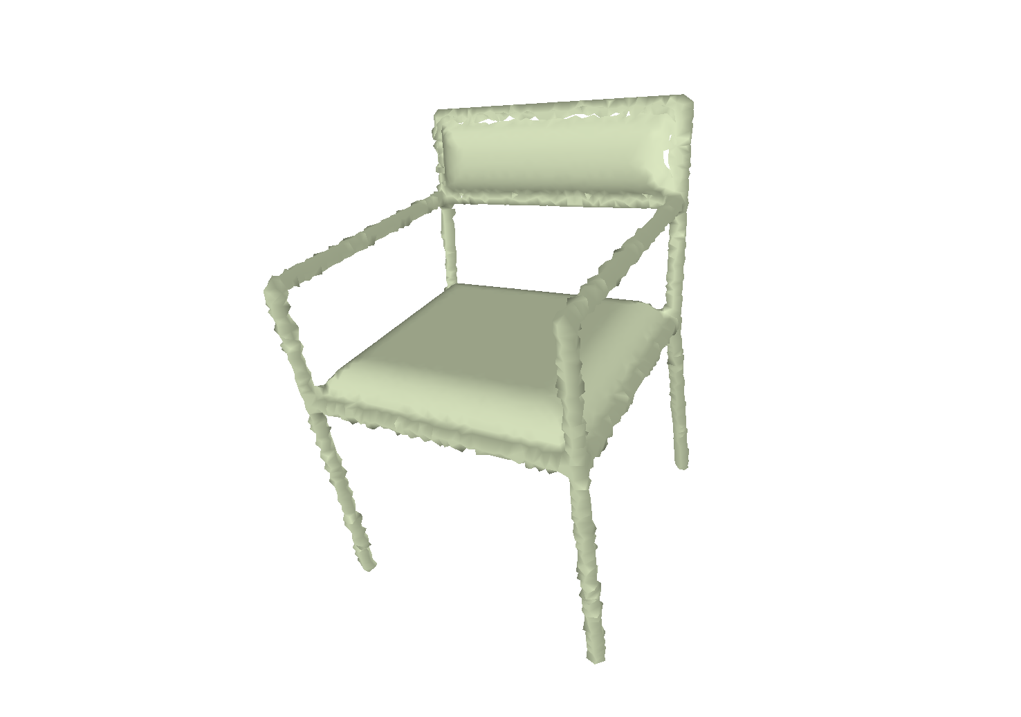
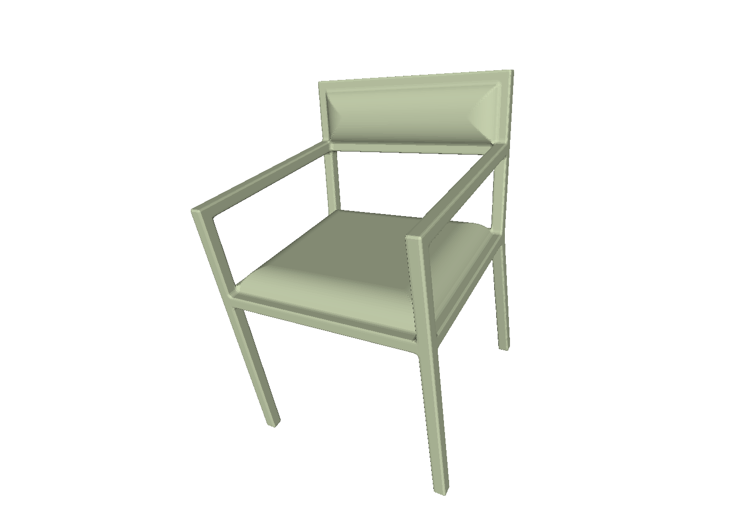
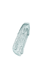
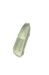
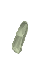
To understand the effects of sparse input on the reconstruction quality, we evaluated IPVNet and the baseline using an input density of $N\sim\{300,3000,10000\}$ points while fixing the voxel resolution to $M=256$. In contrast to the baseline, IPVNet can reconstruct thin structures more accurately and preserve small gaps (Fig. 5 inset images) while quantitatively outperforming the reconstruction with different input densities (Table 1). Furthermore, we investigated IPVNet’s ability to perform closed-surface reconstruction on preprocessed watertight meshes using 13 subsets of ShapeNet for training. The reconstruction results are shown in Fig. 6.

	Chamfer-$L_{2}\downarrow$			$F$-score $\uparrow$
	$N=300$	$N=3000$	$N=10000$	$d=0.1\%$	$d=0.05\%$
NDF	$1.550$	$0.324$	$0.092$	$0.711$	$0.460$
IPVNet	$\mathbf{1.217}$	$\mathbf{0.119}$	$\mathbf{0.068}$	$\mathbf{0.785}$	$\mathbf{0.542}$

Table 1: A quantitative comparison between IPVNet and NDF [2] on the ShapeNet Cars [55] dataset for object reconstruction from different input densities. IPVNet outperforms NDF on all input densities. The chamfer-$L_{2}$ results are of order $\times 10^{-4}$ and the reconstruction results using an input density of $N=10000$ were used to calculate the F-score.

	Chamfer-$L_{2}\downarrow$			$F$-score0.05 $\uparrow$
	$64^{3}$	$128^{3}$	$256^{3}$	$64^{3}$	$128^{3}$	$256^{3}$
NDF	$1.549$	$0.266$	$0.029$	$0.289$	$0.591$	$0.994$
GIFS	$5.245$	$1.210$	$0.141$	$0.240$	$0.510$	$0.891$
IPVNet	$\mathbf{1.441}$	$\mathbf{0.162}$	$\mathbf{0.023}$	$\mathbf{0.335}$	$\mathbf{0.803}$	$\mathbf{0.995}$

Table 2: A quantitative comparison between NDF [2], GIFS [33], and IPVNet on the Garments [57] dataset for object reconstruction at different voxel resolutions. IPVNet outperforms the baselines by significant margin in lower resolutions. The point density was fixed to $N=3K$ for this experiment. The chamfer-$L_{2}$ results are of order $\times 10^{-4}$.

(a)

(b)

(c)

(d)

(e)

(f)

Fig. 6: Reconstruction of closed surfaces from the ShapeNet [55] dataset. From left to right, each triplet represents the input, reconstruction, and ground truth, respectively.

5.3 Real-world scene reconstruction

(a) Input

(b) NDF

(c) IPVNet

(d) IPVNet${}_{\text{mesh}}$

(e) GT

(f)

(g)

(h)

(i)

(j)

(k)

(l)

(m)

(n)

(o)

(p)

(q)

(r)

(s)

(t)

Fig. 7: Scene reconstruction on the test set of the Gibson Environment [1] dataset using NDF [2], IPVNet, and the respective ground truth (GT). Each odd row represents an outside view of a scene while the even rows depict inside views. In contrast to the baseline, IPVNet produces significantly less outliers (outside view) and improves the preservation of geometric features (inset images).

Fig. 8: A qualitative comparison between NDF [2], GIFS [33], and IPVNet on the Garments [57] dataset.

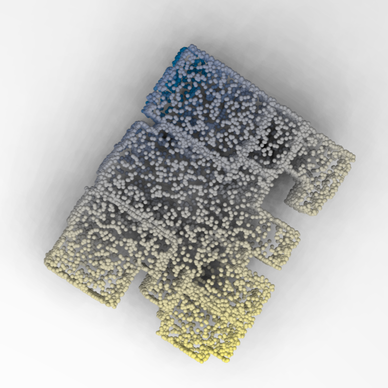
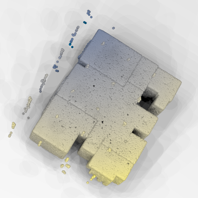
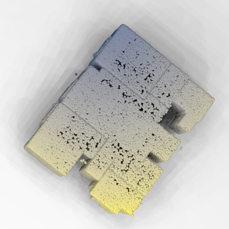
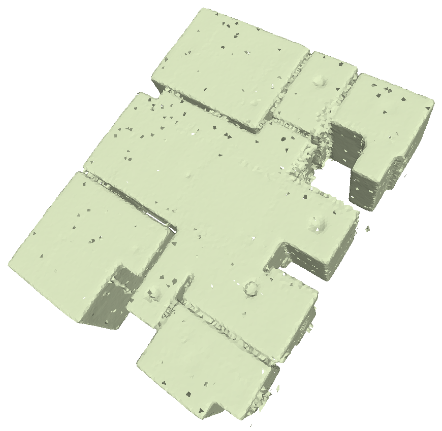
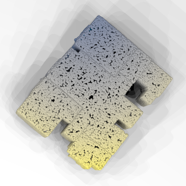
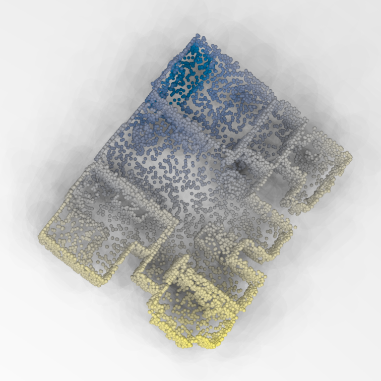
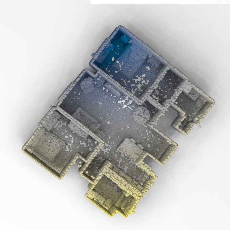
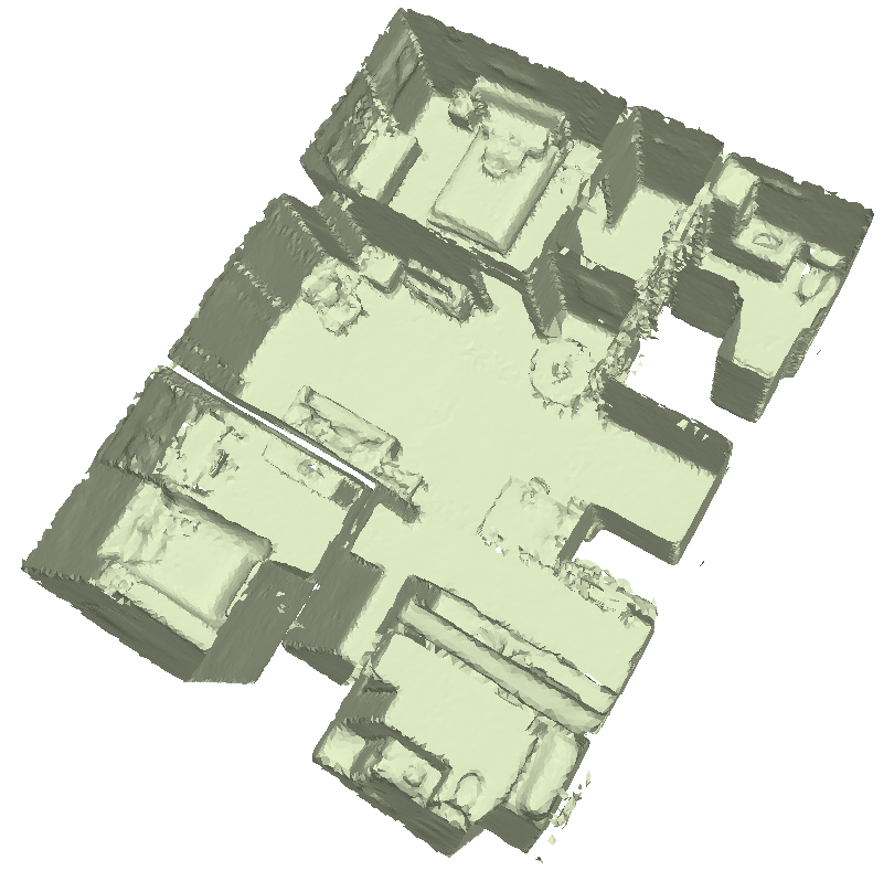
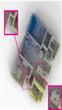
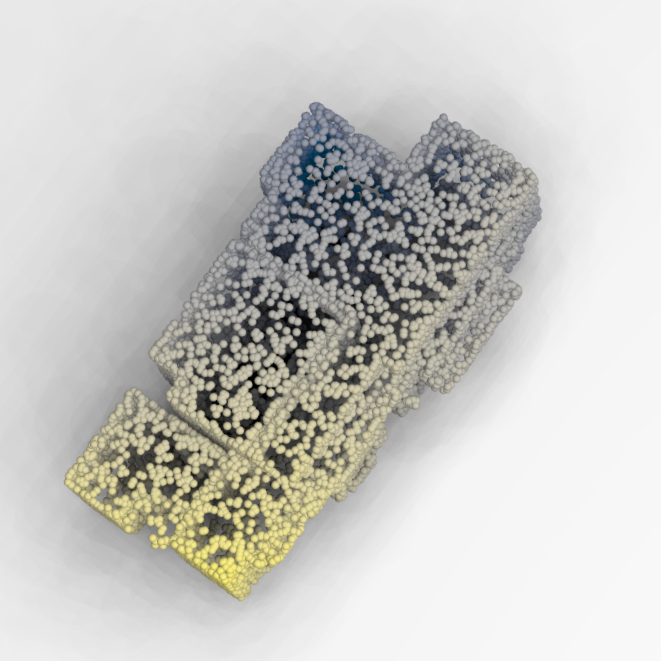
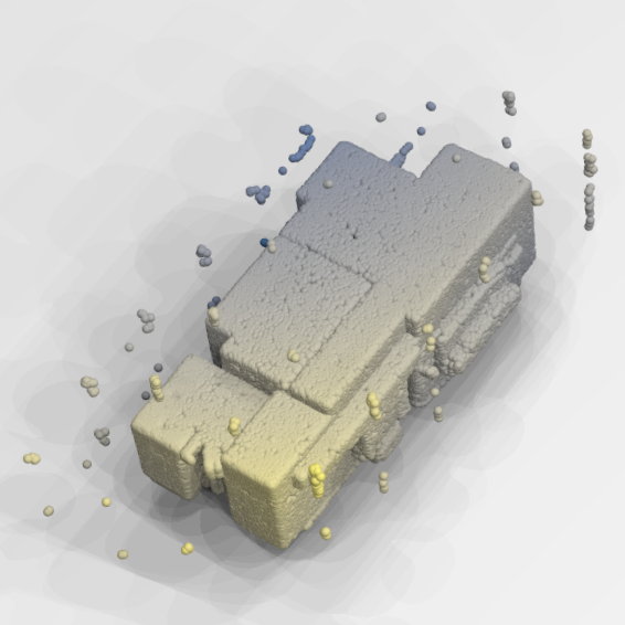
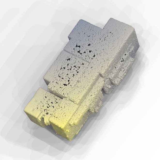
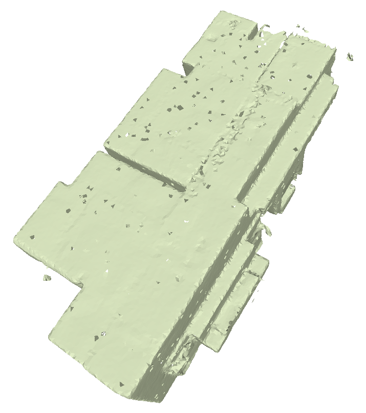
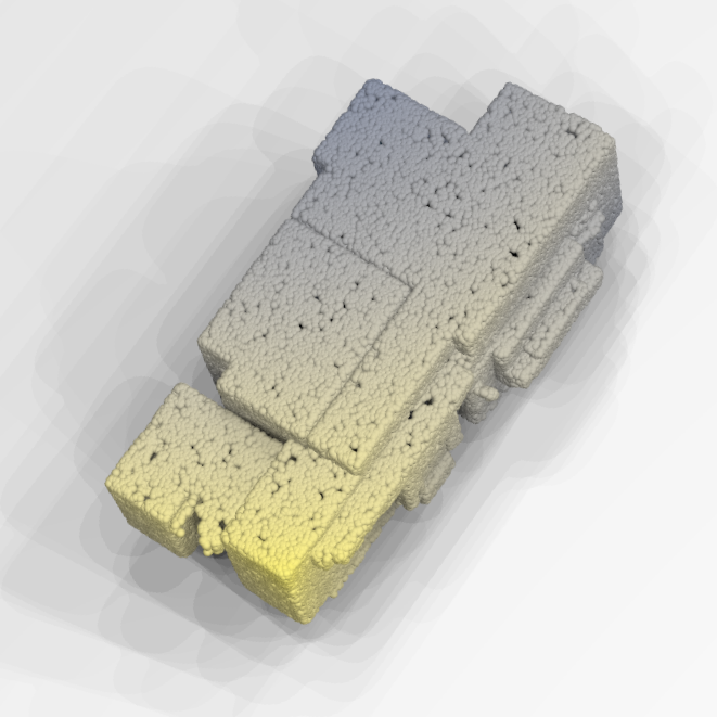
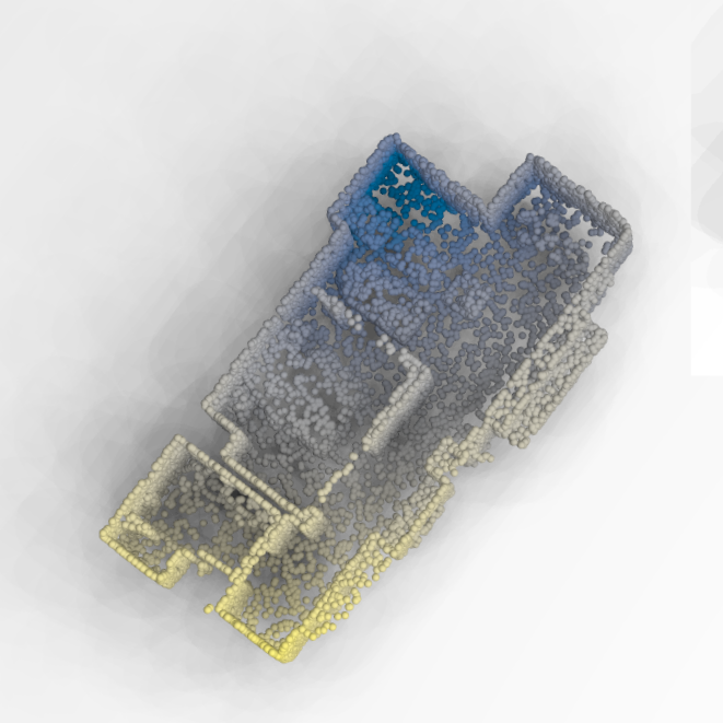
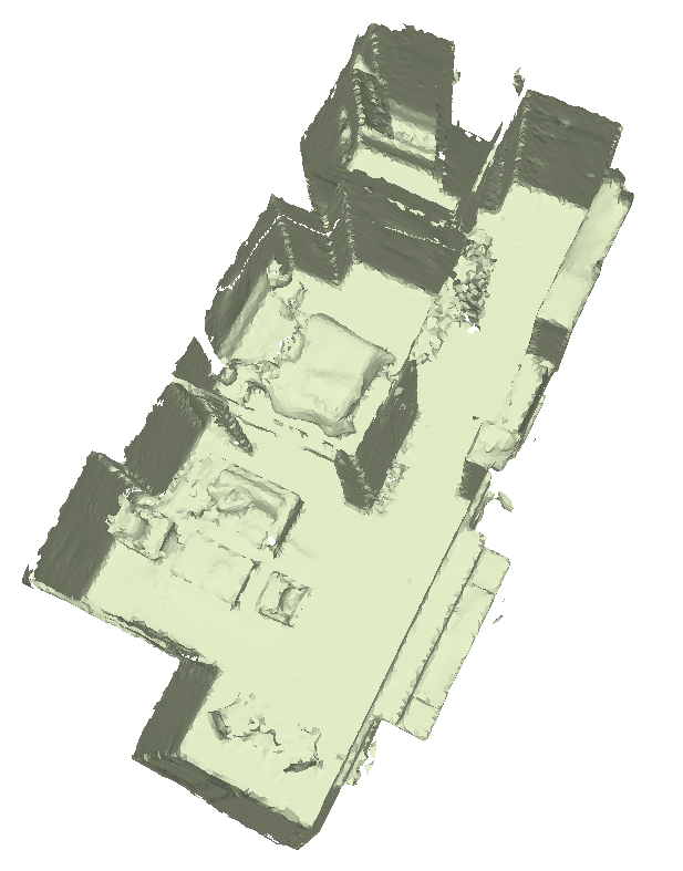
We evaluated the reconstruction of complex real-world scenes through the use of the Gibson Environment dataset [1]. The dataset consists of RGBD scans of indoor spaces. A subset of 35 and 100 scenes were prepared following the procedure from [2] for training and testing, respectively. We utilized a sliding window scheme and reconstructed the surface bounded by each window. Since the sliding window may frequently consist of a very small area of the scene with only few points, we used an output density five times as large the input density (i.e., $\mathcal{O}=5\times N$) to save time. The grid resolutions were kept fixed at $M=256$ for both IPVNet and the baseline. The reconstruction results are highlighted in Fig. 7. In addition to improving the preservation of structural details, IPVNet produces significantly fewer outliers than the baseline due to the use of point features during training and inference.

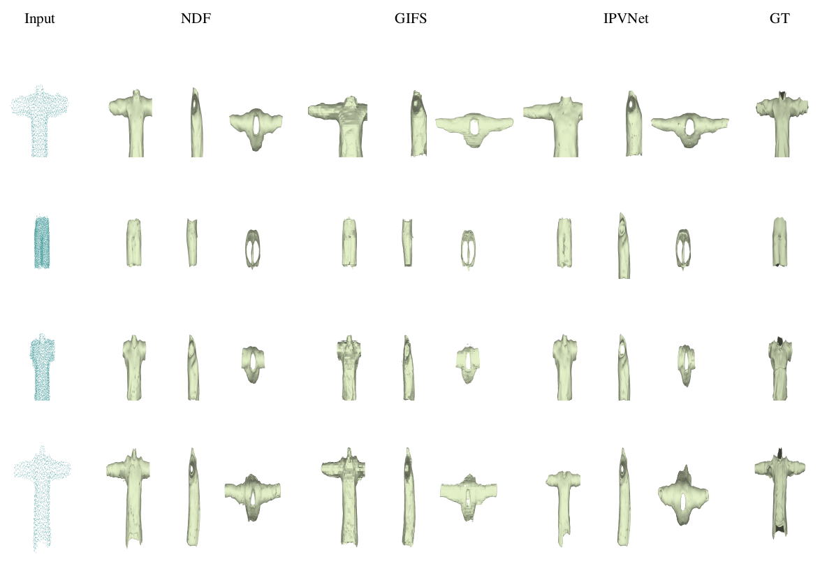
Lastly, we tested IPVNet on the challenging complex surfaces of the Garments [57] dataset. Fig. 8 and Table 2 show the qualitative and quantitative results, respectively. It can be observed from Table 2 that IPVNet exhibits superior performance compared to the baselines, particularly at low grid resolutions. The point-voxel fusion technique utilized by our model is able to effectively recover lost details from the resulting discretization.

6 Ablation study

In this section, we study the effect of different design choices and how they influence the performance of IPVNet on the task of 3D reconstruction.

6.1 Effect of point features on object reconstruction

Since multiple points within the boundary of a grid are merged together in low resolutions, we test the effect of this information loss on object reconstruction. To understand if the point features are helpful in recovering missing information, we trained a version of IPVNet named IPVNet${}_{\text{wp}}$, which has the same neural functions except for the point encoder and point-feature aggregation. Both IPVNet and IPVNet${}_{\text{wp}}$ were trained with differing grid resolutions, $M\sim\{32,64,128,256\}$, while using a fixed input point density of $N=10000$. Our findings on the reconstruction of the ShapeNet Cars dataset are illustrated in Table 3. At lower resolutions, where a significant percentage of the raw points are lost due to voxelization, IPVNet outperforms IPVNet${}_{\text{wp}}$ by a notable margin thus indicating the usefulness of point features.

Grid Resolution	$\%$ of Lost Points	Chamfer-$L_{2}\downarrow$
		IPVNet${}_{\text{wp}}$	IPVNet
32	$82\%$	$9.587$	$\mathbf{4.307}$
64	$45\%$	$0.961$	$\mathbf{0.543}$
128	$16\%$	$0.395$	$\mathbf{0.257}$
256	$4\%$	$0.092$	$\mathbf{0.068}$

Table 3: The object reconstruction accuracy for different grid resolutions on the ShapeNet Cars [55] dataset using only voxel features (IPVNet${}_{\text{wp}}$) and point-voxel features (IPVNet). The second column represents the percentage of raw points lost during the voxelization process due to multiple points overlapping in the same grid. In low-resolution grids, IPVNet significantly outperforms IPVNet${}_{\text{wp}}$. The chamfer-$L_{2}$ results are of order $\times 10^{-4}$.

6.2 Effect of point features on scene reconstruction

(a)

(b)

(c)

(d)

Fig. 9: An ablation study showing the effectiveness of point features during training. To reconstruct a scene from the Gibson Environment [1] dataset, we used (a) the NDF [2] baseline and (b) IPVNet${}_{\text{wp}}$ with our inference algorithm (Alg. 1). The IPVNet reconstruction results are shown in (c) and the ground truth is displayed in (d). Notice that Alg. 1 by itself can reduce the number of outliers. However, when point features are included during training, our reconstruction results (c) are closer to the ground truth (d) and achieve more accurate details with far fewer outliers.

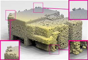
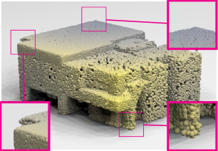
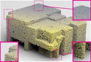
To test the effectiveness of point features on scene reconstruction, we used Alg. 1 to infer the surface for both IPVNet and IPVNet${}_{\text{wp}}$. The reconstruction results are displayed in Fig. 9. Compared to the baseline, Alg. 1 by itself can reduce the number of outliers without point features (Fig. 9b). However, when point features are included during training the reconstruction results (Fig. 9c) are closer to the ground truth (Fig. 9d), and therefore more accurate details with less outliers are realized.

Fig. 10: Reconstruction results after the NDF [2] baseline has been filtered using the input coordinate range as the distance threshold, and IPVNet without any filtering. NDF still includes outliers due to the surface curvature whereas the IPVNet reconstruction consists of significantly less outliers without any filtering.

6.3 Post-processing outlier removal

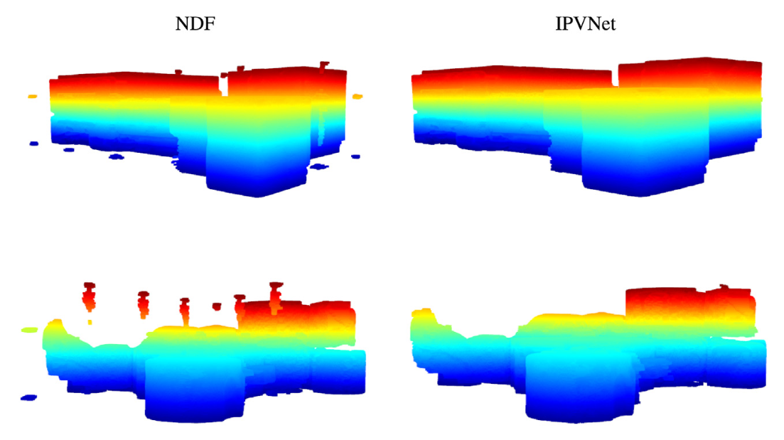
To provide a comparison of IPVNet against a naive post-processing step, we filter the baseline reconstruction using the coordinate range of the input point cloud as the distance threshold. The qualitative results of this experiment are recorded in Fig. 10. It is critical to note that naive post-processing cannot remove all the outliers due to their existence near areas of surface curvature.

7 Limitations and future directions

Despite the fact that the UDF function is capable of reconstructing multiple complex surfaces, the requirement of projecting the query points several times makes the surface inference time long. Our point-voxel formulation may also be beneficial for other implicit techniques such as occupancy and signed distance prediction. We aim to investigate these directions in future work.

8 Conclusion

In this paper we introduced IPVNet, a novel approach that implicitly learns from raw point and voxel features to reconstruct complex open surfaces. To improve the reconstruction quality, we make use of raw point cloud data jointly with voxels to learn local and global features. Not only have we showed that IPVNet outperforms the state of the art on both synthetic and real-world data, but we also demonstrated the effectiveness of point features on 3D reconstruction through ablation studies. Furthermore, we developed an inference module that extracts a zero level set from a UDF and drastically reduces the amount of outliers in the reconstruction. We believe IPVNet is an important step towards reconstructing open surfaces without losing details and introducing outliers, and we hope that our work will inspire more research in this area.

Declaration of competing interests

The authors declare that they have no known competing financial interests or personal relationships that could have appeared to influence the work reported in this paper.

Data availability

Data will be made available on request.

References

- Xia et al. [2018] F. Xia, A. R. Zamir, Z. He, A. Sax, J. Malik, S. Savarese, Gibson env: Real-world perception for embodied agents, in: Proceedings of the IEEE/CVF Conference on Computer Vision and Pattern Recognition, 2018, pp. 9068–9079.
- Chibane et al. [2020] J. Chibane, A. Mir, G. Pons-Moll, Neural unsigned distance fields for implicit function learning, arXiv preprint arXiv:2010.13938 (2020).
- Arshad and Beksi [2020] M. S. Arshad, W. J. Beksi, A progressive conditional generative adversarial network for generating dense and colored 3d point clouds, in: Proceedings of the International Conference on 3D Vision, IEEE, 2020, pp. 712–722.
- Son and Kim [2021] H. Son, Y. M. Kim, Progressive growing of points with tree-structured generators, in: Proceedings of the British Machine Vision Conference, 2021, pp. 1–13.
- Pepe et al. [2022] M. Pepe, V. S. Alfio, D. Costantino, D. Scaringi, Data for 3d reconstruction and point cloud classification using machine learning in cultural heritage environment, Data in Brief 42 (2022) 108250.
- Kim et al. [2023] J. Kim, B.-S. Hua, T. Nguyen, S.-K. Yeung, Pointinverter: Point cloud reconstruction and editing via a generative model with shape priors, in: Proceedings of the IEEE/CVF Winter Conference on Applications of Computer Vision, 2023, pp. 592–601.
- IPVNet [2023] IPVNet, 2023. https://github.com/robotic-vision-lab/Implicit-Point-Voxel-Features-Network.
- You et al. [2020] C. C. You, S. P. Lim, S. C. Lim, J. San Tan, C. K. Lee, Y. M. J. Khaw, A survey on surface reconstruction techniques for structured and unstructured data, in: Proceedings of the IEEE Conference on Open Systems, 2020, pp. 37–42.
- Mescheder et al. [2019] L. Mescheder, M. Oechsle, M. Niemeyer, S. Nowozin, A. Geiger, Occupancy networks: Learning 3d reconstruction in function space, in: Proceedings of the IEEE/CVF Conference on Computer Vision and Pattern Recognition, 2019, pp. 4460–4470.
- Peng et al. [2020] S. Peng, M. Niemeyer, L. Mescheder, M. Pollefeys, A. Geiger, Convolutional occupancy networks, in: Proceedings of the European Conference on Computer Vision, Springer, 2020, pp. 523–540.
- Chen and Zhang [2019] Z. Chen, H. Zhang, Learning implicit fields for generative shape modeling, in: Proceedings of the IEEE/CVF Conference on Computer Vision and Pattern Recognition, 2019, pp. 5939–5948.
- Michalkiewicz et al. [2019] M. Michalkiewicz, J. K. Pontes, D. Jack, M. Baktashmotlagh, A. Eriksson, Deep level sets: Implicit surface representations for 3d shape inference, arXiv preprint arXiv:1901.06802 (2019).
- Littwin and Wolf [2019] G. Littwin, L. Wolf, Deep meta functionals for shape representation, in: Proceedings of the IEEE/CVF International Conference on Computer Vision, 2019, pp. 1824–1833.
- Park et al. [2019] J. J. Park, P. Florence, J. Straub, R. Newcombe, S. Lovegrove, Deepsdf: Learning continuous signed distance functions for shape representation, in: Proceedings of the IEEE/CVF Conference on Computer Vision and Pattern Recognition, 2019, pp. 165–174.
- Genova et al. [2020] K. Genova, F. Cole, A. Sud, A. Sarna, T. Funkhouser, Local deep implicit functions for 3d shape, in: Proceedings of the IEEE/CVF Conference on Computer Vision and Pattern Recognition, 2020, pp. 4857–4866.
- Sitzmann et al. [2020] V. Sitzmann, J. Martel, A. Bergman, D. Lindell, G. Wetzstein, Implicit neural representations with periodic activation functions, in: Proceedings of the Advances in Neural Information Processing Systems, volume 33, 2020, pp. 7462–7473.
- Bhatnagar et al. [2020] B. L. Bhatnagar, C. Sminchisescu, C. Theobalt, G. Pons-Moll, Combining implicit function learning and parametric models for 3d human reconstruction, in: Proceedings of the European Conference on Computer Vision, Springer, 2020, pp. 311–329.
- Chibane et al. [2020] J. Chibane, T. Alldieck, G. Pons-Moll, Implicit functions in feature space for 3d shape reconstruction and completion, in: Proceedings of the IEEE/CVF Conference on Computer Vision and Pattern Recognition, 2020, pp. 6970–6981.
- Atzmon and Lipman [2020a] M. Atzmon, Y. Lipman, Sal: Sign agnostic learning of shapes from raw data, in: Proceedings of the IEEE/CVF Conference on Computer Vision and Pattern Recognition, 2020a, pp. 2565–2574.
- Atzmon and Lipman [2020b] M. Atzmon, Y. Lipman, Sald: Sign agnostic learning with derivatives, arXiv preprint arXiv:2006.05400 (2020b).
- Gropp et al. [2020] A. Gropp, L. Yariv, N. Haim, M. Atzmon, Y. Lipman, Implicit geometric regularization for learning shapes, arXiv preprint arXiv:2002.10099 (2020).
- Mi et al. [2020] Z. Mi, Y. Luo, W. Tao, Ssrnet: scalable 3d surface reconstruction network, in: Proceedings of the IEEE/CVF Conference on Computer Vision and Pattern Recognition, 2020, pp. 970–979.
- Sitzmann et al. [2020] V. Sitzmann, E. R. Chan, R. Tucker, N. Snavely, G. Wetzstein, Metasdf: Meta-learning signed distance functions, arXiv preprint arXiv:2006.09662 (2020).
- Tretschk et al. [2020] E. Tretschk, A. Tewari, V. Golyanik, M. Zollhöfer, C. Stoll, C. Theobalt, Patchnets: Patch-based generalizable deep implicit 3d shape representations, in: Proceedings of the European Conference on Computer Vision, Springer, 2020, pp. 293–309.
- Jiang et al. [2020] C. Jiang, A. Sud, A. Makadia, J. Huang, M. Nießner, T. Funkhouser, Local implicit grid representations for 3d scenes, in: Proceedings of the IEEE/CVF Conference on Computer Vision and Pattern Recognition, 2020, pp. 6001–6010.
- Liu et al. [2021] S.-L. Liu, H.-X. Guo, H. Pan, P.-S. Wang, X. Tong, Y. Liu, Deep implicit moving least-squares functions for 3d reconstruction, in: Proceedings of the IEEE/CVF Conference on Computer Vision and Pattern Recognition, 2021, pp. 1788–1797.
- Huang et al. [2021] J. Huang, S.-S. Huang, H. Song, S.-M. Hu, Di-fusion: Online implicit 3d reconstruction with deep priors, in: Proceedings of the IEEE/CVF Conference on Computer Vision and Pattern Recognition, 2021, pp. 8932–8941.
- Duggal et al. [2021] S. Duggal, Z. Wang, W.-C. Ma, S. Manivasagam, J. Liang, S. Wang, R. Urtasun, Secrets of 3d implicit object shape reconstruction in the wild, arXiv preprint arXiv:2101.06860 (2021).
- Zhao et al. [2021a] W. Zhao, J. Lei, Y. Wen, J. Zhang, K. Jia, Sign-agnostic implicit learning of surface self-similarities for shape modeling and reconstruction from raw point clouds, in: Proceedings of the IEEE/CVF Conference on Computer Vision and Pattern Recognition, 2021a, pp. 10256–10265.
- Zhao et al. [2021b] F. Zhao, W. Wang, S. Liao, L. Shao, Learning anchored unsigned distance functions with gradient direction alignment for single-view garment reconstruction, in: Proceedings of the IEEE/CVF International Conference on Computer Vision, 2021b, pp. 12674–12683.
- Venkatesh et al. [2021] R. Venkatesh, T. Karmali, S. Sharma, A. Ghosh, R. V. Babu, L. A. Jeni, M. Singh, Deep implicit surface point prediction networks, in: Proceedings of the IEEE/CVF International Conference on Computer Vision, 2021, pp. 12653–12662.
- Chen et al. [2022] W. Chen, C. Lin, W. Li, B. Yang, 3psdf: Three-pole signed distance function for learning surfaces with arbitrary topologies, in: Proceedings of the IEEE/CVF Conference on Computer Vision and Pattern Recognition, 2022, pp. 18522–18531.
- Ye et al. [2022] J. Ye, Y. Chen, N. Wang, X. Wang, Gifs: Neural implicit function for general shape representation, in: Proceedings of the IEEE/CVF Conference on Computer Vision and Pattern Recognition, 2022, pp. 12829–12839.
- Xie et al. [2018] J. Xie, Z. Zheng, R. Gao, W. Wang, S.-C. Zhu, Y. N. Wu, Learning descriptor networks for 3d shape synthesis and analysis, in: Proceedings of the IEEE/CVF Conference on Computer Vision and Pattern Recognition, 2018, pp. 8629–8638.
- Le and Duan [2018] T. Le, Y. Duan, Pointgrid: A deep network for 3d shape understanding, in: Proceedings of the IEEE/CVF Conference on Computer Vision and Pattern Recognition, 2018, pp. 9204–9214.
- Huang et al. [2019] W. Huang, B. Lai, W. Xu, Z. Tu, 3d volumetric modeling with introspective neural networks, in: Proceedings of the AAAI Conference on Artificial Intelligence, volume 33, 2019, pp. 8481–8488.
- Liu et al. [2019] Z. Liu, H. Tang, Y. Lin, S. Han, Point-voxel cnn for efficient 3d deep learning, arXiv preprint arXiv:1907.03739 (2019).
- Li et al. [2019] Y. Li, G. Tong, X. Li, L. Zhang, H. Peng, Mvf-cnn: Fusion of multilevel features for large-scale point cloud classification, IEEE Access 7 (2019) 46522–46537.
- Shi et al. [2020] S. Shi, C. Guo, L. Jiang, Z. Wang, J. Shi, X. Wang, H. Li, Pv-rcnn: Point-voxel feature set abstraction for 3d object detection, in: Proceedings of the IEEE/CVF Conference on Computer Vision and Pattern Recognition, 2020, pp. 10529–10538.
- Shi et al. [2021] S. Shi, L. Jiang, J. Deng, Z. Wang, C. Guo, J. Shi, X. Wang, H. Li, Pv-rcnn++: Point-voxel feature set abstraction with local vector representation for 3d object detection, arXiv preprint arXiv:2102.00463 (2021).
- Cui and Zhang [2020] Z. Cui, Z. Zhang, Pvf-net: Point & voxel fusion 3d object detection framework for point cloud, in: Proceedings of the Conference on Computer and Robot Vision, IEEE, 2020, pp. 125–133.
- Tang et al. [2020] H. Tang, Z. Liu, S. Zhao, Y. Lin, J. Lin, H. Wang, S. Han, Searching efficient 3d architectures with sparse point-voxel convolution, in: Proceedings of the European Conference on Computer Vision, Springer, 2020, pp. 685–702.
- Noh et al. [2021] J. Noh, S. Lee, B. Ham, Hvpr: Hybrid voxel-point representation for single-stage 3d object detection, in: Proceedings of the IEEE/CVF Conference on Computer Vision and Pattern Recognition, 2021, pp. 14605–14614.
- Zhang et al. [2021] C. Zhang, H. Wan, S. Liu, X. Shen, Z. Wu, Pvt: Point-voxel transformer for 3d deep learning, arXiv preprint arXiv:2108.06076 (2021).
- Wei et al. [2021] Y. Wei, Z. Wang, Y. Rao, J. Lu, J. Zhou, Pv-raft: point-voxel correlation fields for scene flow estimation of point clouds, in: Proceedings of the IEEE/CVF Conference on Computer Vision and Pattern Recognition, 2021, pp. 6954–6963.
- Li et al. [2021] Y. Li, S. Yang, Y. Zheng, H. Lu, Improved point-voxel region convolutional neural network: 3d object detectors for autonomous driving, IEEE Transactions on Intelligent Transportation Systems (2021).
- Xu et al. [2021] J. Xu, R. Zhang, J. Dou, Y. Zhu, J. Sun, S. Pu, Rpvnet: A deep and efficient range-point-voxel fusion network for lidar point cloud segmentation, in: Proceedings of the IEEE/CVF International Conference on Computer Vision, 2021, pp. 16024–16033.
- Cherenkova et al. [2020] K. Cherenkova, D. Aouada, G. Gusev, Pvdeconv: Point-voxel deconvolution for autoencoding cad construction in 3d, in: Proceedings of the IEEE International Conference on Image Processing, 2020, pp. 2741–2745.
- Nair and Hinton [2010] V. Nair, G. E. Hinton, Rectified linear units improve restricted boltzmann machines, in: Proceedings of the International Conference on Machine Learning, 2010, pp. 807–814.
- Ioffe and Szegedy [2015] S. Ioffe, C. Szegedy, Batch normalization: Accelerating deep network training by reducing internal covariate shift, in: Proceedings of the International Conference on Machine Learning, 2015, pp. 448–456.
- Jaderberg et al. [2015] M. Jaderberg, K. Simonyan, A. Zisserman, K. Kavukcuoglu, Spatial transformer networks, in: Proceedings of the Advances in Neural Information Processing Systems, volume 28, 2015, pp. 1–9.
- Wolter [1993] F.-E. Wolter, Cut locus and medial axis in global shape interrogation and representation, design laboratory memorandum 92-2, 1993.
- Kingma and Ba [2014] D. P. Kingma, J. Ba, Adam: A method for stochastic optimization, arXiv preprint arXiv:1412.6980 (2014).
- Tatarchenko et al. [2019] M. Tatarchenko, S. R. Richter, R. Ranftl, Z. Li, V. Koltun, T. Brox, What do single-view 3d reconstruction networks learn?, in: Proceedings of the IEEE/CVF Conference on Computer Vision and Pattern Recognition, 2019, pp. 3405–3414.
- Chang et al. [2015] A. X. Chang, T. Funkhouser, L. Guibas, P. Hanrahan, Q. Huang, Z. Li, S. Savarese, M. Savva, S. Song, H. Su, J. Xiao, L. Yi, F. Yu, Shapenet: An information-rich 3d model repository, arXiv preprint arXiv:1512.03012 (2015).
- Bernardini et al. [1999] F. Bernardini, J. Mittleman, H. Rushmeier, C. Silva, G. Taubin, The ball-pivoting algorithm for surface reconstruction, IEEE Transactions on Visualization and Computer Graphics 5 (1999) 349–359.
- Bhatnagar et al. [2019] B. L. Bhatnagar, G. Tiwari, C. Theobalt, G. Pons-Moll, Multi-garment net: Learning to dress 3d people from images, in: Proceedings of the IEEE/CVF International Conference on Computer Vision, 2019, pp. 5420–5430.