On Learning the Distribution of a Random Spatial Field in a Location-Unaware Mobile Sensing Setup

Abstract

In applications like environment monitoring and pollution control, physical quantities are modeled by spatio-temporal fields. It is of interest to learn the statistical distribution of such fields as a function of space, time or both. In this work, our aim is to learn the statistical distribution of a spatio-temporal field along a fixed one dimensional path, as a function of spatial location, in the absence of location information. Spatial field analysis, commonly done using static sensor networks is a well studied problem in literature. Recently, due to flexibility in setting the spatial sampling density and low hardware cost, owing to larger spatial coverage, mobile sensors are used for this purpose. The main challenge in using mobile sensors is their location uncertainty. Obtaining location information of samples requires additional hardware and cost. So, we consider the case when the spatio-temporal field along the fixed length path is sampled using a simple mobile sensing device that records field values while traversing the path without any location information. We ask whether it is possible to learn the statistical distribution of the field, as a function of spatial location, using samples from the location-unaware mobile sensor under some simple assumptions on the field. We answer this question in affirmative and provide a series of analytical and experimental results to support our claim.

Keywords Random spatial field  $\cdot$ distribution learning  $\cdot$ location-unaware mobile sensing  $\cdot$ Lipschitz continous spatial field  $\cdot$ bounded spatial field.

1 Introduction

Learning the statistical distribution of spatial (physical) fields is a fundamental task in applications such as environment monitoring and pollution management. Classical solution to this problem includes the usage of a fixed array of sensors, deployed at prime locations over the region of interest (done by agencies like EPA - https://www.epa.gov/). In the past decade, a thorough analysis and some testbeds have proposed the usage of mobile sensors (see  [1]). A key advantage of a mobile sensor is that its infrastructure cost is lower and facilitates higher density of samples. A major challenge in using mobile sensors is the uncertainty of sample locations. With a global positioning system (GPS) receiver, the location can be estimated. However, this information requires extra cost in terms of hardware and battery. The knowledge of location can also have privacy implications on the mobile sensor or its experiments (see  [2]). That is, localization of sensors in MSNs can cost extra energy and hardware (see  [3, 4, 5, 6]).

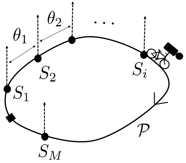
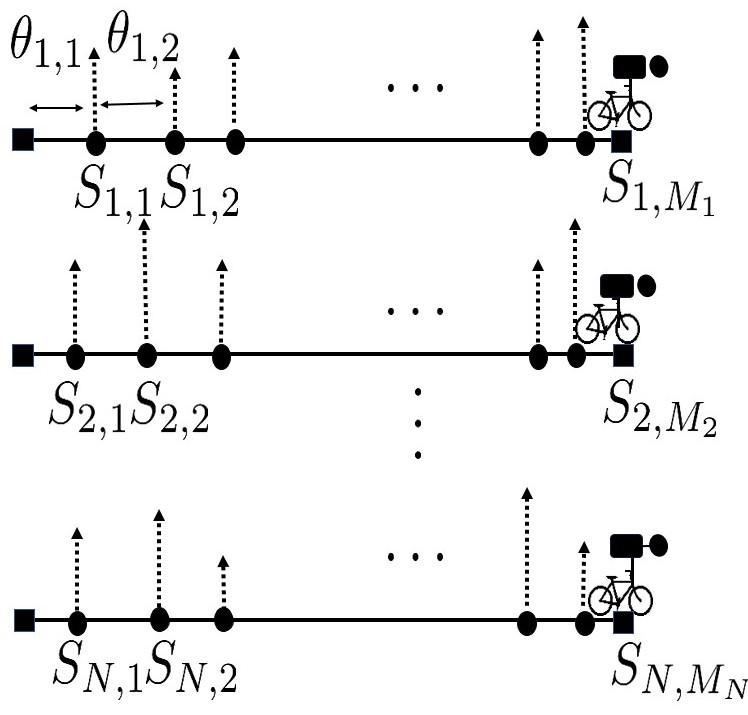
In this work, a spatial field $X(s,t)$ is considered for analysis where $s\in{\cal P}$ is the location on a finite-length path ${\cal P}$ and $t\in{\mathbb{R}}$ is time. It is assumed that the field is bounded in $[-b,b]$ for a finite $b>0$ and is Lipschitz continuous; that is $|X(s,t)-X(s^{\prime},t)|\leq\alpha|s-s^{\prime}|$ for a finite and fixed $\alpha>0$. Learning the statistical distribution of the field $X(s,t)$ as a function of $s$ along the path ${\cal P}$ using samples from a location-unaware mobile sensor is of interest. The sampling locations are unknown and modeled by an unknown renewal process as done in a location-unaware mobile sensing setup in  [7]. Let sampling locations be $S_{1},S_{2},\ldots,S_{M}$ along the path ${\cal P}$, where $M$ is the random number of samples obtained during a mobile-sensing experiment. The inter-sample intervals $\theta_{1}:=S_{1}$, $\theta_{2}:=S_{2}-S_{1},\ldots$ are independent and identically distributed in our model. By unknown renewal process, it is implied that the distribution of $\theta_{1}$ is not known.

The proposed distribution-learning of the spatial field is designed around $N$ experiments of the mobile sensing experiment along path ${\cal P}$. It is assumed that the obtained samples of the spatial-field, as well as the unknown randomly distributed sampling locations, are statistically independent between different experiments. The samples from the same experiment may be dependent or independent, but this assumption is not used in our subsequent analysis. Using the location-unaware samples from $N$ independent experiments, the statistical distribution of $X(s,t)$ for any point $s\in{\cal P}$ has to be learned. The main results of this work are as follows:

1. We design a cumulative distribution function (CDF) estimand for $X(s,t),\quad s\in{\cal P}$ with the maximum error between the estimand and the underlying CDF of $X(s,t),s\in{\cal P}$ is of the order $\mathcal{O}\left(\frac{1}{\sqrt{n}}\right)$. This result holds when the number of experiments $N\rightarrow\infty$.

2. When the number of experimental trials $N$ is finite, we design a CDF estimand for $X(s,t)$, $s\in{\cal P}$ such that the maximum error between the estimand and the underlying CDF of $X(s,t)$, $s\in{\cal P}$ is of the order $\mathcal{O}\left(\frac{1}{\sqrt{n}}+\frac{1}{\sqrt{N}}\right)$ with probability at least $1-\delta$ for any $\delta>0$.

3. Using custom experiments with a handheld sound-meter and acoustic noise measurements along a bounded length path, a data set was created to validate the distribution learning method. The experimental results compare distribution-learning with a fixed and a mobile sound-level probe.

(a)

(b)

Figure 1: (a) Mobile sensor moving along the fixed length 1-D path ${\cal P}$. The field samples are obtained at unknown locations $S_{1}$, $S_{2},\ldots,S_{M}$. (b) N trials of mobile sensing experiment are carried on N different days. Spatial field values are recorded at unknown locations $S_{i,1},S_{i,2},\ldots,S_{i,M_{i}}$ on trial $i$. The number of samples recorded during the $i$th trial is denoted by $M_{i}$.

Prior art: Sampling and reconstruction of spatial fields is an extension of the classical Shannon’s sampling theorem addressed in [8, 9]. Sensing of spatial fields with static/fixed sensor networks is a broadly studied topic studied in [10, 11, 12, 13]. A systematic analysis of spatial field sampling using mobile sensors is reported in [1].

Location-unaware sensing and analysis of spatial fields in the case of static sensors as well as mobile sensors is addressed in literature. Sampling of a bandlimited spatial field at unknown locations is reported in [14, 15, 16]. Sampling of spatially bandlimited fields at unknown but statistically distributed sampling locations is addressed in [17], and [18] studies the optimal probability distribution of sensor locations in this case. It is proved in [19] that reconstruction of polynomial functions can be achieved if unknown sampling locations can be described by an unknown rational function. Bandlimited field reconstruction using location-unaware mobile sensing is addressed in [20, 7]. Spatio-temporal field sampling using location-unaware mobile sensors, where a one dimensional spatial field evolving with time according to a partial differential equation is studied in [21].

In addition to the sampling and reconstruction of spatial fields using a dedicated sensor network, as mentioned above, a study on crowd sensing approach to spatial field sensing is available in literature. Environmental monitoring with smart-phone applications is studied in [22] and vehicular sensor networks is studied in [23], [24].

When the spatial field is random, instead of reconstructing the field, it is of interest to learn the statistical distribution of the spatial field as a function of spatial location. Consider the spatial field $X(s,t)$ varying with time and space. At a given location $s_{0}$, the field value $X(s_{0},t)$ is random. It is of interest to learn the distribution of this random variable. The problem of learning the distribution of a random variable from its samples is a well studied problem in literature (see [25, 26, 27]). However, in our problem, since the sensor is location-unaware, the field is not sampled exactly at the desired location. In such a case, the following sections provide a method to learn the distribution of the spatial field under some simple assumptions.

2 Spatial Field Properties

Let $X(s,t)$ be the spatial field of interest, where $s$ denotes a spatial location and $t$ denotes time. Time $t\in{\mathbb{R}}$ and location $s\in\cal P$, where $\cal P$ denotes a bounded one-dimensional path. Path $\cal P$ can be parameterized by a scalar and it can be normalized to ${\cal P}=[0,1]$. The field is assumed to be bounded in $[-b,b]$ for a finite $b>0$ and Lipschitz continuous w.r.t. $s$; that is

$$|X(s_{1},t)-X(s_{2},t)|\leq\alpha|s_{1}-s_{2}|,$$

where $\alpha>0$ is the Lipschitz constant. Lipschitz continuity indicates that nearby spatial locations have similar field values. The field $X(s,t)$ may not be stationary.

3 Location-Unaware Mobile Sensing Model

The field $X(s,t)$ is sampled using a location-unaware mobile sensor. The sensor moves along the path $\cal P$ and samples the field at regular intervals in time. As the sensor is location-unaware and moves at non-uniform speed, samples are obtained at unknown locations $S_{1},S_{2},\ldots,S_{M}$ along the path ${\cal P}$. The inter-sample intervals are $\theta_{1}:=S_{1}$, $\theta_{2}:=S_{2}-S_{1},\ldots$, $\theta_{M}:=S_{M}-S_{M-1}$. Depending on the time taken to traverse the path $\cal P$, a random number of samples is recorded during a mobile sensing trial. The random number of samples denoted by $M$ is given by a stopping rule (see  [28]):

$$\theta_{1}+\theta_{2}+\ldots+\theta_{M}\leq 1\mbox{ and }\theta_{1}+\theta_{2}+\ldots+\theta_{M+1}>1.$$

The sampling locations are modeled as arrivals of an unknown renewal process. Therefore, $\theta_{1},\theta_{2},\ldots$ are independent and identically distributed. It is assumed that

$$0<\theta\leq\frac{\lambda}{n}\quad\mbox{ and }\quad{\mathbb{E}}(\theta)=\frac{1}{n},$$

where $\lambda>1$ is finite and determined by the maximum sensor speed. The average spatial sampling rate of the sensor is $n$. It is shown in [7] that the conditional average of $\theta$ conditioned on $M=m$ is approximately $\frac{1}{m}$ and

$${\mathbb{E}}[M]\leq n+\lambda-1.$$

A model of mobile sensing experiment is explained next. The field samples are recorded by performing $N$ independent trials of mobile sensing along the path $\cal P$. Let $\vec{X}_{i}$ be the set of field samples collected and let $M_{i}$ be the number of samples recorded during trial $i$. After $N$ trials we obtain

$$\vec{X}_{1} :=[X(S_{1,1},t_{1,1}),X(S_{1,2},t_{1,2}),\ldots,X(S_{1,M_{1}},t_{1,M_{1}})]^{T};$$

$$\ldots,$$

$$\vec{X}_{N} :=\big{[}X(S_{N,1},t_{N,1}),X(S_{N,2},t_{N,2}),$$

$$\hskip 119.50148pt\ldots,X(S_{N,M_{N}},t_{N,M_{N}})\big{]}^{T}.$$

The location and time of the $j$th field value recorded during trial $i$ are given by $S_{i,j}$ and $t_{i,j}$ respectively. These sampling locations for $N$ different trials are generated by the same unknown renewal process. The field values $\vec{X}_{1},\vec{X}_{2}\ldots$ are statistically independent; however, the field values in $\vec{X}_{i}$ for a given trial may be dependent.

4 Distribution Learning of Spatial Field

It is of interest to learn the distribution of the field $X(s,t)$ at a given location $s\in[0,1]$. The field value $X(s,t_{0})$ at location $s$, at time $t_{0}\in{\mathbb{R}}$ is estimated by $\hat{X}(s)$ which is given by,

$$\hat{X}(s)=X\left(s_{\lfloor(M-1)s\rfloor+1},t_{0}\right),$$

where $M$ is the random number of samples recorded along path $\cal P$ and $s_{\lfloor(M-1)s\rfloor+1},t_{0}$ are the location and time at which ${(\lfloor(M-1)s\rfloor+1})^{th}$ sample is recorded respectively. The field samples $\vec{X}_{1},\vec{X}_{2}\ldots\vec{X}_{N}$ are available after $N$ trials of the mobile sensing experiment. The field value at location $s\in{[0,1]}$ for the $i^{th}$ trial is estimated by

$$\hat{X}_{i}(s)=X\left(s_{i,{\lfloor(M_{i}-1)s\rfloor+1}},t_{i,\lfloor(M_{i}-1)s\rfloor+1}\right),$$ (1)

while $X_{i}(s)=X\left(s,t_{i,\lfloor(M_{i}-1)s\rfloor+1}\right)$. For simplicity, the dependence on $t$ has been dropped on the left-hand side as the distribution learning accuracy is governed by the error in estimating sample locations.

Proposition 1.

([29], Theorem 1, Equation (11))

Consider the path ${\cal P}=[0,1]$. Let $S_{1},S_{2},\ldots,S_{M}$ be the unknown sampling locations, and $\theta_{1},\theta_{2},\ldots,\theta_{M}$ be the inter-sample intervals. The sampling locations are points from an unknown renewal process which satisfies ${\mathbb{E}}[\theta_{1}]=\frac{1}{n}$ and $0<\theta\leq\frac{\lambda}{n}$. Then the mean squared error between sampling location $S_{\lfloor(M-1)s\rfloor+1}$ and location $s$ is

$${\mathbb{E}}\left[\left|S_{\lfloor(M-1)s\rfloor+1}-s\right|^{2}\right]\leq((n+\lambda-1)s(1-s)+C)\frac{\lambda^{2}}{n^{2}},$$

where $C$ is a constant.

Proposition 1 shows that the mean squared error between location $s$ on path ${\cal P}$ and the estimated sampling location decreases with increasing spatial sampling rate $n$. The field is assumed to be Lipschitz continuous, so

$$\left|X(s)-\hat{X}(s)\right|\leq\alpha\left|S_{\lfloor(M-1)s\rfloor+1}-s\right|,$$ (2)

where $\alpha$ is the Lipschitz constant. This shows that for a given value of $\alpha$, the error between the field value at location $s$, $X(s)$ and the estimated field value at location $s$, $\hat{X}(s)$ at a given time, depends only on the error in sampling location. Using the Lipschitz property of the field and Proposition 1, a bound on the probability of error in estimating $X(s)$ by $\hat{X}(s)$ is given in [29].

Proposition 2.

([29], Theorem 1, Equation (14) and Theorem 2, Equation (19)) Let $\hat{X}(s)$ be the estimate of the field value at location $s$, estimated using field value sampled at unknown sampling location $S_{\lfloor(M-1)s\rfloor+1}$. Let $M$ be the random number of samples generated by the location-unaware mobile sensor on a finite length path ${\cal P}$. The sampling locations $S_{1},S_{2},\ldots,S_{M}$ are generated by an unknown renewal process, where the inter-sample intervals $\theta_{1},\theta_{2},\ldots\theta_{M}$ are such that ${\mathbb{E}}[\theta_{1}]=\frac{1}{n}$ and $0<\theta\leq\frac{\lambda}{n}$. Then for every $s\in[0,1]$ and for any $\varepsilon>0$,

$${\mathbb{P}}\left(\left|X(s)-\hat{X}(s))\right|>\varepsilon\right)\leq\frac{\alpha^{2}}{\varepsilon^{2}}((n+\lambda-1)s(1-s)+C)\frac{\lambda^{2}}{n^{2}}$$ (3)

and

$${\mathbb{P}}\left(\sup_{s\in[0,1]}\left|\hat{X}(s)-X(s)\right|>\varepsilon\right)\leq\frac{32}{\beta}\frac{\alpha^{2}}{\varepsilon^{2}}(n+\lambda-1)\frac{\lambda^{2}}{n^{2}},$$ (4)

where $\beta$ goes to 1 as $n\to\infty$.

From Proposition 2,  (3) we can see that for a given accuracy level $\varepsilon>0$, probability of the error(absolute difference) between the field value $X(s)$ and its estimate $\hat{X}(s)$ at location $s$, at a given time, being greater than $\varepsilon$ has an upper bound of order $\mathcal{O}(\frac{1}{n})$. For a given $\varepsilon$ this upper bound decreases with increasing spatial sampling rate $n$. In other words, as the sampling rate $n$ tends to infinity, $\hat{X}(s)$ converges to ${X}(s)$. The upper bound in $\eqref{bound_on_sup_prob_prop2}$ implies that as the sampling rate $n$ tends to infinity, $\hat{X}(s)$ converges uniformly over $s\in[0,1]$ to ${X}(s)$. Having obtained the estimated field values $\hat{X}_{1}(s),\hat{X}_{2}(s),\ldots,\hat{X}_{N}(s)$ at location $s$ after $N$ trials, we estimate the cumulative distribution function(CDF) of field value at location $s$, denoted by $F_{\hat{X}(s)}(x)={\mathbb{P}}(\hat{X}(s)\leq x)$. Using the classical Glivenko-Cantelli theorem, the estimated CDF at location $s$, $F_{\hat{X}(s)}(x)$ is obtained as

$$F_{\hat{X}(s)}(x)=\lim_{N\rightarrow\infty}\frac{1}{N}\sum_{i=1}^{N}\mathbb{I}\left(\hat{X}_{i}(s)\leq x\right),$$ (5)

where $\mathbb{I}(.)$ denotes the indicator function. Let CDF of the field value at location $s$ be denoted by

$$F_{X(s)}(x)={\mathbb{P}}(X(s)\leq x).$$

Now, we investigate the difference between the CDF of field value $F_{X(s)}(x)$ at location $s$ and its estimate $F_{\hat{X}(s)}(x)$.

Theorem 1.

Let $M$ be the random number of samples generated when a location-unaware mobile sensor samples the field along the finite length path ${\cal P}$. Let $S_{1},S_{2},\ldots,S_{M}$ be the sampling locations and $\theta_{1},\theta_{2},\ldots\theta_{M}$ be the inter-sample intervals generated by the unknown renewal process such that ${\mathbb{E}}[\theta_{1}]=\frac{1}{n}$ and $0<\theta\leq\frac{\lambda}{n}$. Then for every $x\in{\mathbb{R}},s\in[0,1]$ and for any $\varepsilon>0$,

$$\lvert F_{X(s)}(x)-F_{\hat{X}(s)}(x)\rvert\leq\frac{\alpha^{2}}{\varepsilon^{2}}((n+\lambda-1)s(1-s)+C)\frac{\lambda^{2}}{n^{2}}+2\alpha\max_{x}(f_{X(s)}(x))\frac{\lambda}{n}\sqrt{((n+\lambda-1)s(1-s)+C)}.$$ (6)

Proof.

We can split $F_{\hat{X}(s)}(x)$ as

$$F_{\hat{X}(s)}(x)$$

$$={\mathbb{P}}(\hat{X}(s)\leq x)$$

$$={\mathbb{P}}(\hat{X}(s)\leq x,X(s)\leq x)+{\mathbb{P}}(\hat{X}(s)\leq x,X(s)>x)$$

$$\leq{\mathbb{P}}(X(s)\leq x)+{\mathbb{P}}(\hat{X}(s)\leq x,X(s)>x)$$

$$\leq F_{X(s)}(x)+{\mathbb{P}}(\hat{X}(s)\leq x,X(s)>x+\varepsilon)+{\mathbb{P}}(\hat{X}(s)\leq x,x<X(s)\leq x+\varepsilon).$$

Therefore,

$$\lvert F_{\hat{X}(s)}(x)-F_{X(s)}(x)\rvert\leq\underbrace{{\mathbb{P}}(|\hat{X}(s)-X(s)|>\varepsilon)}_{ft}+\underbrace{{\mathbb{P}}(\hat{X}(s)\leq x,x<X(s)\leq x+\varepsilon)}_{st}.$$ (7)

An upper bound on ($ft$) is given in Proposition 2, (3). We propose the following lemma that gives an upper bound on ($st$).

Lemma 1.

Let $\hat{X}(s)$ be the estimate of the field value at location $s$, estimated using field value sampled at unknown sampling location $S_{\lfloor(M-1)s\rfloor+1}$. Let $M$ is the random number of samples generated by the location-unaware mobile sensor on a finite length path ${\cal P}$. The sampling locations $S_{1},S_{2},\ldots,S_{M}$ are generated by an unknown renewal process, where the inter-sample intervals $\theta_{1},\theta_{2},\ldots\theta_{M}$ are such that ${\mathbb{E}}[\theta_{1}]=\frac{1}{n}$ and $0<\theta\leq\frac{\lambda}{n}$. Then for every $x\in{\mathbb{R}},s\in[0,1]$ and for any $\varepsilon>0$,

$${\mathbb{P}}(\hat{X}(s)\leq x,x<X(s)\leq x+\varepsilon)\leq 2\alpha\max_{x}(f_{X(s)}(x))\frac{\lambda}{n}\sqrt{((n+\lambda-1)s(1-s)+C)},$$

where $f_{X(s)}$ is the probability density function of the field value at location $s$.

Proof.

A detailed proof of Lemma 1 is given in Appendix A. Owing to the Lipschitz nature of the field, from (2) it holds that if $\hat{X}(s)\leq x$, then $X(s)\leq x+\alpha\left|S_{\lfloor(M-1)s\rfloor+1}-s\right|$. So,

$${\mathbb{P}}(\hat{X}(s)\leq x,x<X(s)\leq x+\varepsilon)\leq{\mathbb{P}}(x<X(s)\leq x+Z),$$

where $Z=\min\left(\varepsilon,\alpha\left|S_{\lfloor(M-1)s\rfloor+1}-s\right|\right)$. From Proposition 1, the mean squared error between $s$ and its estimate $S_{\lfloor(M-1)s\rfloor+1}$ is of order $\mathcal{O}(\frac{1}{n})$. Thus it is shown in Appendix A that ${\mathbb{E}}[Z]$ has an upper bound of order $\mathcal{O}(\frac{1}{\sqrt{n}})$ and ${\mathbb{P}}(x<X(s)\leq x+Z)$ is bounded from above by $2\alpha\max_{x}(f_{X(s)}(x))\frac{\lambda}{n}\sqrt{((n+\lambda-1)s(1-s)+C)}$, which is independent of $\varepsilon$. ∎

The Lemma follows by substituting the upper bound on ($ft$) and ($st$) in (7). ∎

The upper bound given in the RHS of (6) has two terms. The first term increases with decreasing value of $\varepsilon$ and the second term is of order $\mathcal{O}\left(\frac{1}{\sqrt{n}}\right)$. Thus, Theorem 1 implies that the upper bound on the pointwise absolute difference between the CDF of field value, $F_{X(s)}(x)$ and its estimate, $F_{\hat{X}(s)}(x)$, at location $s$, is at least of order $\mathcal{O}\left(\frac{1}{\sqrt{n}}\right)$. The value of $\varepsilon$ can be chosen such that the upper bound in (6) is of order $\mathcal{O}\left(\frac{1}{\sqrt{n}}\right)$. For example if $\varepsilon=n^{-\frac{1}{4}}$,

$$\lvert F_{\hat{X}(s)}(x)-F_{X(s)}(x)\rvert \leq\alpha^{2}\sqrt{n}((n+\lambda-1)s(1-s)+C)\frac{\lambda^{2}}{n^{2}}$$

$$\hskip 150.79968pt+2\alpha\max_{x}(f_{X(s)}(x))\frac{\lambda}{n}\sqrt{((n+\lambda-1)s(1-s)+C)}.$$

As the spatial sampling rate $n$ tends to infinity, the upper bound on the error in estimation of CDF in (6) tends to zero for some $\varepsilon>0$. Thus, $F_{\hat{X}(s)}(x)$ converges to $F_{X(s)}(x)$ as $n$ tends to infinity. The upper bound given in the RHS of (6) depends on $s$ and has a maximum at $s=1/2$. By taking supremum over $s$ we get,

$$\sup_{s\in[0,1]}\lvert F_{\hat{X}(s)}(x)-F_{X(s)}(x)\rvert\leq\frac{\alpha^{2}}{\varepsilon^{2}}\left(\frac{(n+\lambda-1)}{4}+C\right)\frac{\lambda^{2}}{n^{2}}+2\alpha\max_{x,s}(f_{X(s)}(x))\frac{\lambda}{n}\sqrt{\left(\frac{(n+\lambda-1)}{4}+C\right)}.$$

This implies that as the sampling rate $n$ tends to infinity, for some $\varepsilon>0$, $F_{\hat{X}(s)}(x)$ converges uniformly over $s\in[0,1]$ to $F_{X(s)}(x)$.

Theorem 1 gives an upper bound on the error between $F_{X(s)}(x)$ and its estimate $F_{\hat{X}(s)}(x)$, defined in (5) for number of trials $N\to\infty$. However, the number of trials $N$ is finite in practice. The field values $\vec{X}_{1},\vec{X}_{2},\ldots,\vec{X}_{N}$ are obtained after $N$ trials of the mobile sensing experiment. The field value at a given location $s$ on path ${\cal P}$, for trial $i$ is estimated by $\hat{X_{i}}(s)$ given in (1). Using $N$ estimates of the field value, the empirical CDF at location $s$ is

$$F_{\hat{X}(s),N}(x)=\frac{1}{N}\sum_{i=1}^{N}\mathbb{I}\left(\hat{X}_{i}(s)\leq x\right).$$ (8)

Theorem 2.

Let $M$ be the random number of samples generated when a location-unaware mobile sensor samples the field along the finite length path ${\cal P}$. Let $S_{1},S_{2},\ldots,S_{M}$ be the sampling locations and $\theta_{1},\theta_{2},\ldots\theta_{M}$ be the inter-sample intervals generated by the unknown renewal process such that ${\mathbb{E}}[\theta_{1}]=\frac{1}{n}$ and $0<\theta\leq\frac{\lambda}{n}$. Then for every $x\in{\mathbb{R}},s\in[0,1]$ and for any $\delta>0$,

$$\sup_{x\in{\mathbb{R}}}\lvert F_{\hat{X}(s),N}(x)-F_{X(s)}(x)\rvert\leq\frac{A^{2}}{\varepsilon^{2}}+2\max_{x}(f_{X(s)}(x))A+\sqrt{\frac{\log(\frac{2}{\delta})}{2N}}$$ (9)

with probability at least $1-\delta$, where $A=\alpha\sqrt{((n+\lambda-1)s(1-s)+C)}\frac{\lambda}{n}$.

Proof.

The error in estimation of $F_{X(s)}(x)$ using finite number of samples is

$${\mathbb{P}}\left(\sup_{x\in{\mathbb{R}}}\lvert F_{\hat{X}(s),N}(x)-F_{X(s)}(x)\rvert>\xi\right)\leq{\mathbb{P}}\Big{(}\sup_{x\in{\mathbb{R}}}\lvert F_{\hat{X}(s),N}(x)-F_{\hat{X}(s)}(x)\rvert+\sup_{x\in{\mathbb{R}}}\lvert F_{\hat{X}(s)}(x)-F_{X(s)}(x)\rvert>\xi\Big{)}.$$ (10)

The upper bound on error in CDF estimation given in Theorem 1, (6) is $\frac{A^{2}}{\varepsilon^{2}}+2\max_{x}(f_{X(s)}(x))A$, where $A=\alpha\sqrt{((n+\lambda-1)s(1-s)+C)}\frac{\lambda}{n}$. Substituting the upper bound in (10) gives,

$${\mathbb{P}}\left(\sup_{x\in{\mathbb{R}}}\lvert F_{\hat{X}(s),N}(x)-F_{X(s)}(x)\rvert>\xi\right)\leq{\mathbb{P}}\Big{(}\sup_{x\in{\mathbb{R}}}\lvert F_{\hat{X}(s),N}(x)-F_{\hat{X}(s)}(x)\rvert>\xi-\frac{A^{2}}{\varepsilon^{2}}-2\max_{x}(f_{X(s)}(x))A\Big{)}.$$

By applying DKW inequality (from [30]) to RHS of above equation we get

$${\mathbb{P}}\left(\sup_{x\in{\mathbb{R}}}\lvert F_{\hat{X}(s),N}(x)-F_{X(s)}(x)\rvert>\xi\right)\leq 2e^{-2N{\left(\xi-\frac{A^{2}}{\varepsilon^{2}}-2\max_{x}(f_{X(s)}(x))A\right)}^{2}}.$$

If $\delta=2e^{-2N{\left(\xi-\frac{A^{2}}{\varepsilon^{2}}-2\max_{x}(f_{X(s)}(x))A\right)}^{2}}$, then $\xi=\frac{A^{2}}{\varepsilon^{2}}+2\max_{x}(f_{X(s)}(x))A+\sqrt{\frac{\log(\frac{2}{\delta})}{2N}}$. Thus,

$${\mathbb{P}}\left(\sup_{x\in{\mathbb{R}}}\lvert F_{\hat{X}(s),N}(x)-F_{X(s)}(x)\rvert>\xi\right)\leq\delta.$$

Thus, the theorem follows from the above inequality. ∎

The upper bound on the RHS of (9), in Theorem 2, comprises of three terms. The first two terms constitute the upper bound on the pointwise absolute error between $F_{X(s)}(x)$ and its estimate $F_{\hat{X}(s)}(x)$ given in Theorem 1. The value of $\varepsilon$ can be chosen such that it is of order $\mathcal{O}(\frac{1}{\sqrt{n}})$. The third term is of order $\mathcal{O}(\frac{1}{\sqrt{N}})$. Thus, Theorem 2 implies that, the supremum of the pointwise absolute error between $F_{X(s)}(x)$ and its estimate $F_{\hat{X}(s),N}(x)$, taken over $x$, is less than an upper bound of order $\mathcal{O}\left(\frac{1}{\sqrt{n}}+\frac{1}{\sqrt{N}}\right)$ with probability atleast $1-\delta$. Thus, the error in estimating $F_{X(s)}(x)$ by $F_{\hat{X}(s),N}(x)$ decreases with the increasing spatial sampling rate $n$ and the number of trials $N$. Increasing the spatial sampling rate leads to better estimation of field values, whereas increasing the number of trials reduces the error in learning the CDFs using their empirical estimates.

In Section 5 we verify our claim by running our distribution learning method on a simulated spatio-temporal field. Using a custom generated dataset we verify the performance of our distribution learning method in section 6.

5 Simulation of Distribution Learning Method with Samples from Location-Unaware Mobile Sensor

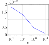
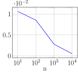
In this section, we apply our distribution learning method to learn the distribution of a simulated spatio-temporal field $X(s,t)$. We sample this field at locations generated by a renewal process and estimate the CDF of field value at some point $s\in[0,1]$ using these samples. A spatio-temporal field $X(s,t)$ is generated, where

$$X(s,t)=a_{0}+\sum_{k=1}^{5}a_{k}(t)cos(2\pi kfs).$$

The constants $a_{0}=500$, $f=5$ and $a_{k}$ is a uniform random variable whose parameter is a function of time $t$. The field $X(s,t)$ is a summation of cosine functions varying with spatial locations having time varying amplitudes. It is of interest to learn the CDF of field value at location $s$, $F_{X(s)}$. However, $N$ trials of the location-unaware mobile sensing experiment are simulated and we can only learn the empirical CDF $F_{X(s),N}$ using $N$ samples of $X(s,t)$ at location $s$. Let $m_{i}$ be the random number of samples generated during trial $i$, where $i=1,2,\ldots,N$. Let $s_{i,1},s_{i,2},\ldots,s_{i,m_{i}}$ be the randomly generated sampling locations and $t_{i,1},t_{i,2},\ldots,t_{i,m_{i}}$ be the sampling times for trial $i$. Sampling location for trial $i$ and sample $j$ is $s_{i,j}=\sum_{l=1}^{j}\theta_{i,l}$, where $\theta_{i,l}$ is the intersample interval generated by a Triangular distribution with mean $\frac{1}{n}$, lower limit $0$ and upper limit $\frac{2}{n}$. Let $k=\lfloor(M-1)s\rfloor+1$. For the $i^{th}$ trial, the sample at sampling location $s_{i,k}$, $\hat{X}_{i}(s)=X(s_{i,k},t_{i,k})$ is the estimate of the field value $X_{i}(s)=X(s,t_{i,k})$ at location $s$. We compare the empirical CDFs $F_{X(s),N}(x)=\frac{1}{N}\sum_{i=1}^{N}\mathbb{I}\left(X_{i}(s)\leq x\right)$ and $F_{\hat{X}(s),N}(x)$ given in (8).

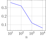
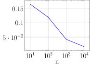
Location-unaware mobile sensing experiment is simulated for $N=50$ and $N=500$ and for spatial sampling rates $n=10,100,1000$ and $10000$ samples/m. The experiment is repeated 200 times for each value of $N$ and $n$. Average absolute pointwise difference in CDF, avg${}_{x}{\left|F_{X(s),N}(x)-F_{\hat{X}(s),N}(x)\right|}$ and maximum absolute pointwise difference in CDF, $\max_{x}|F_{X(s),N}(x)-F_{\hat{X}(s),N}(x)|$ are averaged over 200 iterations for each value of $N$ and $n$.

(a)

(b)

Figure 2: Average absolute pointwise difference in CDF, avg${}_{x}{\left|F_{X(s),N}(x)-F_{\hat{X}(s),N}(x)\right|}$ plotted for different values of $n$ and (a) $N=50$ and (b) $N=500$.

(a)

(b)

Figure 3: Maximum absolute pointwise difference in CDF, $\max_{x}|F_{X(s),N}(x)-F_{\hat{X}(s),N}(x)|$ plotted for different values of $n$ and (a) $N=50$ and (b) $N=500$.

The results are plotted in Figure 2 and Figure 3 where we observe that as the spatial sampling rate increases the error in CDF estimation of field samples as a function of spatial location decreases. We also observe that the error in CDF estimation decreases with the number of trials $N$.

6 Acoustic Noise Distribution Learning Experiment with a Location-Unaware Mobile Soundmeter

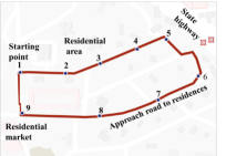
In this section, an experiment is designed to validate the distribution learning method. The mobile sensing experiment is performed along a fixed length path ${\cal P}_{1}$ shown in the map in Figure 4. The field value measured is the acoustic-noise level along path ${\cal P}_{1}$. A sound level meter measuring acoustic-noise level every second is carried along the path. Path ${\cal P}_{1}$ is a closed path along which there is a substantial variation in the acoustic-noise levels. It is not necessary for the path to be closed but it has to be of fixed length. Sound level meter by BAFX products (Model no: BAFX3608) is used in the experiment. Its specifications are given in Table 1. It has memory to store data but does not have any GPS or localization tool.

Table 1: Specifications of Sound Meter.

Range: 30-130dB	Sampling Rate: 1 per sec
Memory: 4700 readings	Accuracy: $\pm$ 1.5 dB

Figure 4: Path along which acoustic noise levels are recorded. The locations marked in the map with numbers are used for measurement using a fixed sensor.

The sound level meter measures one sample per second. The distance between locations of two different samples on ${\cal P}_{1}$ depends on the speed at which the sound level meter traverses the path. Thus by varying the sensor speed, the average spatial sampling rate $n$ of the sound level meter is varied. The sound level meter is moved along path ${\cal P}_{1}$ at two different average speeds to get two different data sets.

Figure 5: Scatter plot of acoustic noise levels along the path ${\cal P}_{1}$ in Figure 4 for each trial in Data set 1.

Figure 6: Box plot plotted using samples from the mobile sound level meter in Data set 1 along the path ${\cal P}_{1}$ in Figure 4 of length 1015m.

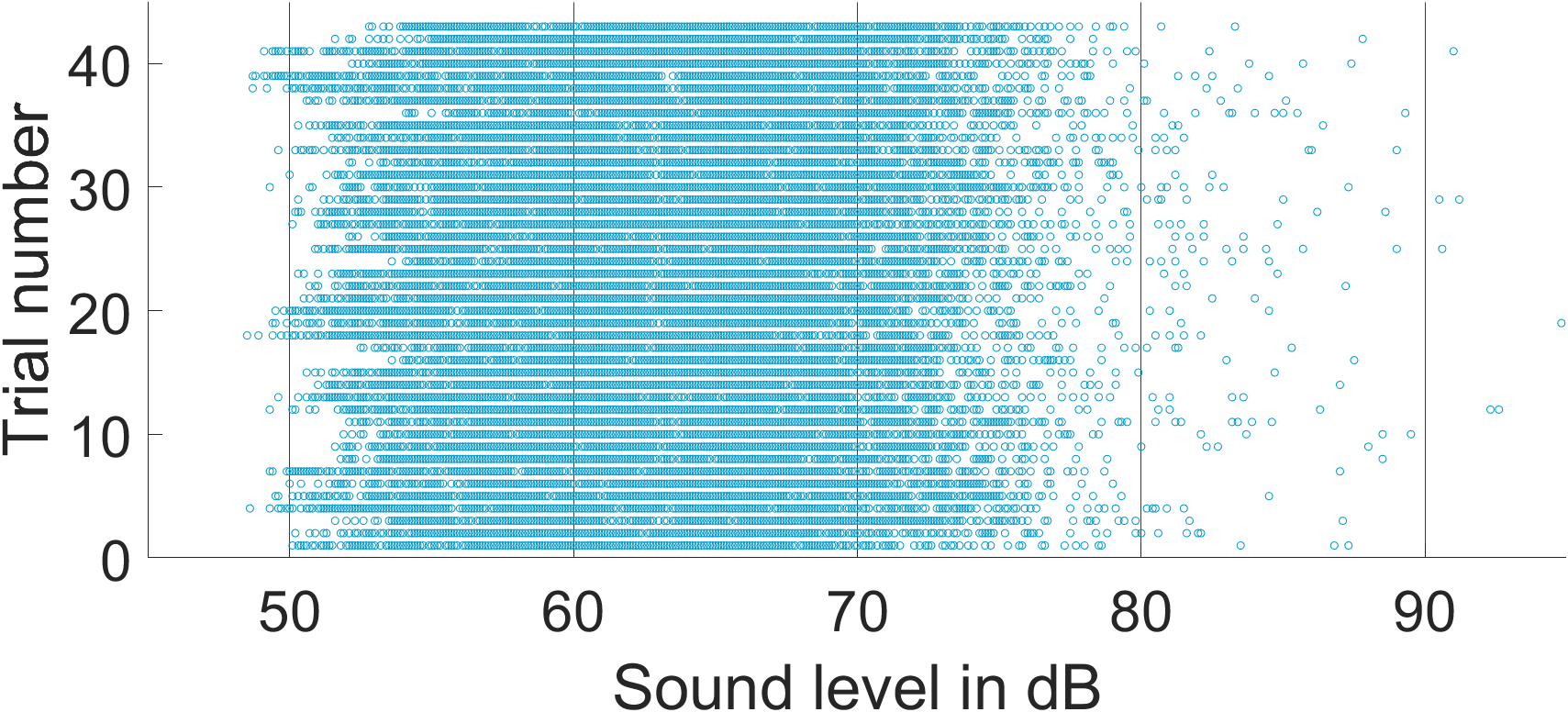
Data sets: Data set 1 was created by walking along path ${\cal P}_{1}$ with the sound level meter. The trials of this experiment were performed 43 times along the same path on different days. Let $n_{1}$ be the average spatial sampling rate for Data set 1. Data set 2 was created by cycling along path ${\cal P}_{1}$ with the sound level meter. In this case as well 43 trials were performed along the same path on different days. Let $n_{2}$ be the average spatial sampling rate for Data set 2. Faster the sensor speed, lower will be the spatial sampling rate of the mobile sensor, sampling at the uniform rate in time. Therefore,

$$n_{2}<n_{1}.$$

The number of trials performed N=43. The samples obtained in Data set 1 and Data set 2 can be used to estimate the CDF of acoustic noise levels at locations marked by numbers one to nine on path ${\cal P}_{1}$ as shown in Figure 4 using (8). Since the CDF of sound levels at a given location on path ${\cal P}_{1}$ is not know, a static sound level meter was used to measure acoustic noise levels at locations marked with numbers one to nine along path ${\cal P}_{1}$ shown in Figure 4. These samples are used to compute the empirical CDF of acoustic noise levels at the numbered locations on path ${\cal P}_{1}$. The CDF computed at a numbered location along path ${\cal P}_{1}$ using samples from the fixed sensor is compared with the CDF computed using Data set 1 and Data set 2 at that location.

(a)

(b)

Figure 7: Comparison of empirical CDF of sound levels obtained by experimentation at location 9 along path ${\cal P}_{1}$ in Figure 4, for two different sampling rates of mobile sensor: (a) fixed sensor versus mobile sensor for Data set 1 (Higher spatial sampling rate $n_{1}$) (b) fixed sensor versus mobile sensor for Data set 2 (Lower spatial sampling rate $n_{2}$).

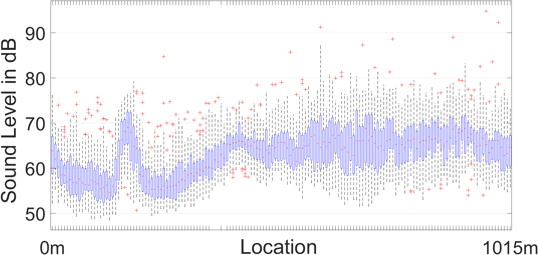
The range, median and quartiles of acoustic noise levels along path ${\cal P}_{1}$ can be visualised using a box plot illustrated in Figure 6. The variation in average noise level is about 20 dB (ratio of 100) while the variation in dynamic range exceeds 30dB (ratio of 1000). Figure 5 shows the variation of acoustic noise levels during each trial of the mobile sensing experiment in Data set 1

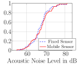
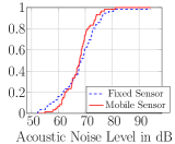
In Figure 7, the distribution learning method is compared for two different spatial sampling rates $n_{1}$ and $n_{2}$. The maximum absolute pointwise error in learning the empirical CDFs in Figure 7a is less than the maximum absolute pointwise error between the empirical CDFs in Figure 7b. This shows that the error in learning the empirical CDFs is lower for Data set 1 having higher spatial sampling rate compared to Data set 2. This validates our theoritical claims. Through experiments we have verified the impact of spatial sampling rate on distribution learning. However, due to limited amount of data, the effect of increasing the number of trials is not investigated in the experiment.

7 Conclusion

We have proposed a data-driven method for learning the statistical distribution of a time-varying spatial field as a function of spatial location under some simple assumptions. A bounded and Lipschitz continuous time varying spatial field is sampled using a location-unaware mobile sensor. The unknown sampling locations are modeled by an unknown renewal process. We have shown that the error in learning the distribution of field value as a function of space decreases with increasing spatial sampling rate $n$ of the location-unaware mobile sensor and number of trials of the mobile sensing experiment $N$. (i) We have a bound of $\mathcal{O}\left(\frac{1}{\sqrt{n}}\right)$ on the maximum error in estimating the CDF of the spatial field, as a function of spatial location. This is an improvement over the bound of $\mathcal{O}\left(\frac{1}{n^{1/3}}\right)$ given in [29]. This bound holds as $N$ goes to infinity. (ii) In addition, we show that with probability atleast $1-\delta$, the error in estimating the CDF of the spatial field as a function of spatial location is of $\mathcal{O}\left(\frac{1}{\sqrt{n}}+\frac{1}{\sqrt{N}}\right)$ for a finite $N$. We validate this claim using simulations. We have created a data set with 43 trials of the mobile sensing experiment measuring acoustic noise levels along a fixed length path using a location-unaware mobile sound level meter. The experimental results also validate the distribution learning method.

Appendix A

Proof of Lemma 1: The field is assumed to be Lipschitz continuous, so

$$|X(s)-\hat{X}(s)|\leq\alpha\left|S_{\lfloor(M-1)s\rfloor+1}-s\right|=\alpha D,$$ (11)

where $D=\left|S_{\lfloor(M-1)s\rfloor+1}-s\right|$. From (11) we can write,

$$X(s)-\alpha D\leq\hat{X}(s).$$

So,

$${\mathbb{P}}(\hat{X}(s)\leq x,x<X(s)\leq x+\varepsilon) \leq{\mathbb{P}}(X(s)-\alpha D\leq x,x<X(s)\leq x+\varepsilon)$$

$$={\mathbb{P}}(x<X(s)\leq x+\min(\alpha D,\varepsilon)).$$

Let the random variable $Z=\min(\alpha D,\varepsilon)$. The conditional probability that $X(s)$ lies between $x$ and $x+Z$, given $Z=z$, is

$${\mathbb{P}}(x<X(s)\leq x+Z|Z=z)\leq z\max_{x}(f_{X(s)}(x)).$$ (12)

Probability that $X(s)$ lies between $x$ and $x+Z$ is given by

$${\mathbb{P}}(x<X(s)\leq x+Z)={\mathbb{E}}[{\mathbb{P}}(x<X(s)\leq x+Z|Z)],$$ (13)

where expectation is taken over $Z$. From (12) and (13) we get

$${\mathbb{P}}(x<X(s)\leq x+Z)\leq{\mathbb{E}}[Z]\max_{x}(f_{X(s)}(x)).$$ (14)

The random variable $Z=\min(\alpha D,\varepsilon)$ can be written as

$$Z=\varepsilon.\mathbb{I}(\alpha D>\varepsilon)+\alpha D.\mathbb{I}(\alpha D\leq\varepsilon),$$

where $\mathbb{I}(.)$ denotes the indicator function. The conditional expectation of $Z$ given $D$ is

$${\mathbb{E}}[Z|D=d]=\varepsilon.\mathbb{I}(\alpha d>\varepsilon)+\alpha d.\mathbb{I}(\alpha d\leq\varepsilon).$$

So,

$${\mathbb{E}}[Z] =\varepsilon.\underbrace{{\mathbb{P}}(\alpha D>\varepsilon)}_{*}+{\mathbb{E}}[\alpha D].{\mathbb{P}}(\alpha D\leq\varepsilon).$$

By applying Markov inequality on (*) we get

$${\mathbb{E}}[Z] \leq{\mathbb{E}}[\alpha D]+{\mathbb{E}}[\alpha D].{\mathbb{P}}(\alpha D\leq\varepsilon)$$

$$={\mathbb{E}}[\alpha D](1+{\mathbb{P}}(\alpha D\leq\varepsilon))$$

$$\leq 2{\mathbb{E}}[\alpha D].$$ (15)

By Jensen’s inequality, $({\mathbb{E}}[\alpha D])^{2}\leq{\mathbb{E}}[\alpha^{2}D^{2}]$. From Proposition 1 we have

$${\mathbb{E}}[\alpha^{2}D^{2}]\leq\alpha^{2}((n+\lambda-1)s(1-s)+C)\frac{\lambda^{2}}{n^{2}}.$$

Therefore,

$${\mathbb{E}}[\alpha D]\leq\alpha\frac{\lambda}{n}\sqrt{((n+\lambda-1)s(1-s)+C)}.$$

By substituting the above upper bound in (15) we get

$${\mathbb{E}}[Z]\leq 2\alpha\frac{\lambda}{n}\sqrt{((n+\lambda-1)s(1-s)+C)}.$$

By substituting the upper bound on ${\mathbb{E}}[Z]$ in (14) we get

$${\mathbb{P}}(\hat{X}(s)\leq x,x<X(s)\leq x+\varepsilon)\leq 2\alpha\max_{x}(f_{X(s)}(x))\frac{\lambda}{n}\sqrt{((n+\lambda-1)s(1-s)+C)}.$$

References

- [1] J. Unnikrishnan and M. Vetterli. Sampling and reconstruction of spatial fields using mobile sensors. IEEE Transactions on Signal Processing, 61(9):2328–2340, May 2013.
- [2] Y. Lin, Y. Ye, and Y. Yang. Preserving incumbent user’s location privacy against environmental sensing capability. In 2019 IEEE International Symposium on Dynamic Spectrum Access Networks (DySPAN), pages 1–10, 2019.
- [3] X. Che, I. Wells, P. Kear, G. Dickers, X. Gong, and M. Rhodes. A static multi-hop underwater wireless sensor network using rf electromagnetic communications. In 2009 29th IEEE International Conference on Distributed Computing Systems Workshops, pages 460–463, June 2009.
- [4] Lingxuan Hu and David Evans. Localization for mobile sensor networks. In Proceedings of the 10th annual international conference on Mobile computing and networking, pages 45–57. ACM, 2004.
- [5] Y. Lin, H. Tao, Y. Tu, and T. Liu. A node self-localization algorithm with a mobile anchor node in underwater acoustic sensor networks. IEEE Access, 7:43773–43780, 2019.
- [6] C. L. Nguyen and U. Raza. Localization of wsns using a location-unaware uav. In ICC 2019 - 2019 IEEE International Conference on Communications (ICC), pages 1–7, 2019.
- [7] A. Kumar. On bandlimited field estimation from samples recorded by a location-unaware mobile sensor. IEEE Transactions on Information Theory, 63(4):2188–2200, April 2017.
- [8] A. J. Jerri. The Shannon Sampling Theorem – its Various Extensions and Applications: a Tutorial Preview. Proceedings of the IEEE, 65:1565–1594, Nov. 1977.
- [9] Farokh Marvasti. Nonuniform sampling: theory and practice. Springer Science & Business Media, 2012.
- [10] D. Marco, E. J. Duarte-Melo, M. Liu, and D. L. Neuhoff. On the many-to-one transport capacity of a dense wireless sensor network and the compressibility of its data. In IPSN, Proc. of the Intl. Wkshp., Palo Alto, CA, USA, LNCS edited by L. J. Guibas and F. Zhao, Springer, NY, 2003, pages 1–16, 2003.
- [11] R. Nowak, U. Mitra, and R. Willett. Estimating inhomogeneous fields using wireless sensor networks. IEEE Journal on Selected Areas in Communications, 22(6):999–1006, 2004.
- [12] Animesh Kumar, Prakash Ishwar, and Kannan Ramchandran. High-resolution distributed sampling of bandlimited fields with low-precision sensors. IEEE Trans. on Information Theory, 57(1):476–492, Jan. 2011.
- [13] R. M. Willett, A. M. Martin, and R. D. Nowak. Adaptive sampling for wireless sensor networks. In International Symposium onInformation Theory, 2004. ISIT 2004. Proceedings., pages 519–, 2004.
- [14] P. Marziliano and M. Vetterli. Reconstruction of irregularly sampled discrete-time bandlimited signals with unknown sampling locations. IEEE Transactions on Signal Processing, 48(12):3462–3471, Dec 2000.
- [15] A. Nordio, C. Chiasserini, and E. Viterbo. Performance of linear field reconstruction techniques with noise and uncertain sensor locations. IEEE Transactions on Signal Processing, 56(8):3535–3547, Aug 2008.
- [16] G. Elhami, M. Pacholska, B. B. Haro, M. Vetterli, and A. Scholefield. Sampling at unknown locations: Uniqueness and reconstruction under constraints. IEEE Transactions on Signal Processing, 66(22):5862–5874, Nov 2018.
- [17] A. Kumar. On bandlimited signal reconstruction from the distribution of unknown sampling locations. IEEE Transactions on Signal Processing, 63(5):1259–1267, March 2015.
- [18] Ankur Mallick; Animesh Kumar. Bandlimited field reconstruction from samples obtained on a discrete grid with unknown random locations. 2016.
- [19] M. Pacholska, B. B. Haro, A. Scholefield, and M. Vetterli. Sampling at unknown locations, with an application in surface retrieval. In 2017 International Conference on Sampling Theory and Applications (SampTA), pages 364–368, July 2017.
- [20] A. Kumar. Bandlimited field estimation from samples recorded by a location-unaware mobile sensor. In 2016 IEEE International Symposium on Information Theory (ISIT), pages 1257–1261, July 2016.
- [21] S. Salgia and A. Kumar. Bandlimited spatiotemporal field sampling with location and time unaware mobile sensors. In 2018 IEEE International Conference on Acoustics, Speech and Signal Processing (ICASSP), pages 4574–4578, April 2018.
- [22] Judicaël Picaut, Nicolas Fortin, Erwan Bocher, Gwendall Petit, Pierre Aumond, and Gwenaël Guillaume. An open-science crowdsourcing approach for producing community noise maps using smartphones. Building and Environment, 148:20–33, 2019.
- [23] Y. Wang and G. Chen. Efficient data gathering and estimation for metropolitan air quality monitoring by using vehicular sensor networks. IEEE Transactions on Vehicular Technology, 66(8):7234–7248, Aug 2017.
- [24] F. Morselli, F. Zabini, and A. Conti. Environmental monitoring via vehicular crowdsensing. In 2018 IEEE 29th Annual International Symposium on Personal, Indoor and Mobile Radio Communications (PIMRC), pages 1382–1387, Sep. 2018.
- [25] Sudeep Kamath, Alon Orlitsky, Dheeraj Pichapati, and Ananda Theertha Suresh. On learning distributions from their samples. In Peter Grünwald, Elad Hazan, and Satyen Kale, editors, Proceedings of The 28th Conference on Learning Theory, volume 40 of Proceedings of Machine Learning Research, pages 1066–1100, Paris, France, 03–06 Jul 2015. PMLR.
- [26] Alon Orlitsky and Ananda Theertha Suresh. Competitive distribution estimation: Why is good-turing good. Advances in Neural Information Processing Systems, 28:2143–2151, 2015.
- [27] Yi Hao, Ayush Jain, Alon Orlitsky, and Vaishakh Ravindrakumar. Surf: A simple, universal, robust, fast distribution learning algorithm. arXiv preprint arXiv:2002.09589, 2020.
- [28] Rick Durrett. Probability: theory and examples. Cambridge university press, 2010.
- [29] Meera Pai and Animesh Kumar. Distribution learning of a random spatial field with a location-unaware mobile sensor. In H. Wallach, H. Larochelle, A. Beygelzimer, F. d'Alché-Buc, E. Fox, and R. Garnett, editors, Advances in Neural Information Processing Systems 32, pages 12479–12487. Curran Associates, Inc., 2019.
- [30] Pascal Massart. The tight constant in the dvoretzky-kiefer-wolfowitz inequality. The annals of Probability, pages 1269–1283, 1990.
- [31] David Pollard. Convergence of stochastic processes. Springer Science & Business Media, 2012.