SPHEAR: Spherical Head Registration for Complete Statistical 3D Modeling
Abstract
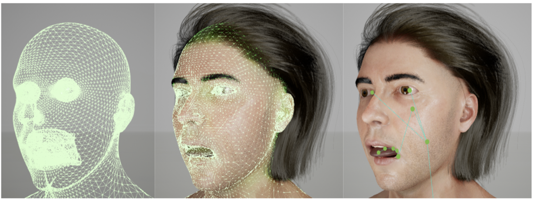
We present SPHEAR, an accurate, differentiable parametric statistical 3D human head model, enabled by a novel 3D registration method based on spherical embeddings. We shift the paradigm away from the classical Non-Rigid Registration methods, which operate under various surface priors, increasing reconstruction fidelity and minimizing required human intervention. Additionally, SPHEAR is a complete model that allows not only to sample diverse synthetic head shapes and facial expressions, but also gaze directions, high-resolution color textures, surface normal maps, and hair cuts represented in detail, as strands. SPHEAR can be used for automatic realistic visual data generation, semantic annotation, and general reconstruction tasks. Compared to state-of-the-art approaches, our components are fast and memory efficient, and experiments support the validity of our design choices and the accuracy of registration, reconstruction and generation techniques.
![[Uncaptioned image]](/html/2311.02461/assets/x1.png)
1 Introduction
Three-dimensional morphable models (3DMMs) of the human face and head have proven highly useful for a variety of computer vision and graphics applications. Since the introduction of the first 3DMMs [10], a palette of expressive models [85, 48, 58, 17, 86] have been developed and deployed in various contexts [26]. Nowadays, 3D face and head models serve as essential building blocks for applications such as 3D avatar creation [28, 43], media creation and editing [76, 75], 3D human reconstruction [69, 97], or synthetic data generation [83], among others.
As the applications of 3DMMs have become more diverse and mature, the demands placed on these models have increased accordingly. However, most current models capture only the 3D geometry of the human face or head, often with limited detail, and neglect appearance entirely or provide only low-frequency texture models for the skin and face. Furthermore, eyes, teeth, the tongue, or hair are frequently missing, which are essential components in the modeling of the human head (see Tab. 1). To enable the aforementioned applications, researchers palliated these missing elements by using, for example, free-form model deformation [43], neural rendering [28], or by relying on artist-designed assets [83, 8].
In building an accurate 3DMM for heads, template registration is a critical first step [85, 48]. During registration, a predefined template is fitted to unstructured and often noisy 3D human head scans, resulting in a representation with consistent topology and semantics that can be used for subsequent statistical model learning. Therefore, since model learning is often based on registered meshes, the registration quality is crucial in achieving optimal model performance. We have found that conventional registration techniques are often insufficiently accurate and sensitive to initialization and parameterization. Therefore, manual intervention and cleaning are typically required during the registration process to develop a reliable model. These limitations are restrictive in two important ways: First, when parameters and initialization are not carefully chosen or manual intervention is not carefully performed, modeling accuracy suffers. Second, the diversity and expressiveness of a model are restricted by the number of scans that can be manually inspected. To develop a model that captures the diversity of humanity, however, a large sample is preferable [12].
In this paper, we take 3DMMs a step further and present SPHEAR, our diverse, holistic model of the human head, that includes a color texture, surface normal maps, and a hair representation compatible with the head geometry. In addition, our model also comprises essential physical components such as eyeballs, a tongue, teeth, and matching assets for facial hair, eyebrows, and eyelashes. To enable the creation of SPHEAR, we present the following contributions: (1) A novel and robust registration pipeline based on a learned spherical embedding, which provides smooth and accurate automatic registrations, agnostic to the template resolution, with preserved semantics and lower error when compared to conventional methods; (2) A non-linear generative shape and expression model for faces, learned on a newly collected 3D dataset of human facial expressions (FHE3D) including eye-balls, teeth and tongue; (3) A fast, flexible, neural generative hair model, that operates in texture space and allows for control of the number of generated strands. Moreover, our proposed Legendre polynomial encoding of hair strands enables smaller models, faster training, and a variable number of control points per strand; (4) For completeness, we also introduce a neural generative appearance model for detailed color and normal maps of human faces; (5) In extensive experiments, we ablate critical design choices and model variants, and demonstrate our model’s accuracy, diversity, and relevance for applications.
† has eyeballs, ‡ has a texture completion model, ∗ vertex-based extension added in subsequent work
2 Related Work
Registration
is the process of accurately deforming a template mesh to fit a scan, and key to learning accurate, realistic statistical head models. Most non-rigid registration methods [48, 85] rely on as conformal as possible (ACAP) registration [89], which we argue does not provide sufficient accuracy to build high quality models. Inspired by spherical template registration [34], that learns a diffeomorphic flow between a sphere and a genus-0 scan, through Neural ODE integration [18], we go one step further and learn the registration between any genus-0 template and any genus-0 scan. [21] learn a diffeomorphism between a genus-0 sphere and the target mesh using a ResNet. They further relax the need for 3D ground truth by learning an illumination model under a reconstruction loss. [55] use an explicit family of bijective functions (i.e. normalizing flows [25, 62]) to model the mapping. In this work, we show how genus-0 sphere mappings can be used for high resolution registration and triangulation, with good generalization and considerable decrease in reconstruction error. Our approach can be viewed as an intrinsic registration method, where alignment is done in the sphere embedding space. But, different from other intrinsic methods, we can easily deform between the template and the scan, in either direction. For a comprehensive survey of the non-rigid registration literature see [24].
Canonical embeddings for 3D representation
Several methods [19, 74, 33, 87, 20] have used canonical representations (e.g spheres, UV spaces, 3D codes) for embedding surfaces or point-clouds. While we share a general learning spirit with [19], we are the first to show how high-density face meshes can be interpolated, matched and registered at sub-millimeter reconstruction error, better than optimization-based, classical registration methods. This is achieved through explicit spherical embeddings, with densely sampled geometry on the mesh surfaces, modulated by high-frequency Siren [70] networks. We design losses such that points can be processed independently/parallel, allowing the networks to learn the high-frequency structures. [19] operates solely on point-clouds ( 2k points), is limited in the number of points it can match, and its spherical embedding formulation is mathematically different. Instead, we operate on dense meshes for registration, where sub-millimeter accuracy is required.
3D morphable face and head models
aim to capture the diverse characteristics of the human face or head in form of 3D geometric models controlled by small dimensional latent parametrizations [26]. Initial work by Blanz and Vetter [10] and the subsequent Basel Face Model [56, 29] represent only the frontal face and ear regions and rely on PCA-based geometry and texture spaces trained on scans from 200 subjects with neutral expression. Subsequent work enriches the shape space with more 3D scans [12, 13, 15] or images from the Internet [42, 14, 27]. Disentangled facial identity and expressions are obtained by bilinear models [80, 17, 11, 86]. More related are full head models, typically trained on a larger and more diverse set of subjects [48, 85, 86, 57, 58], and allowing for separate control over geometry, pose, and expression. While most use 3D scans and sometimes images, SCULPTOR [59] further utilizes CT scans. Deep neural networks have been used to obtain richer non-linear latent representations [7, 2, 61, 78, 77, 79, 85]. Finer textures and sometimes normal maps are obtained using GANs [31] – however, mostly for texture reconstruction or completion [49, 58, 46] and seldom for statistical appearance modeling [47]. Neural fields [84] have been explored more recently [93, 88, 30, 91], sometimes focusing on image quality [37, 81] rather than generative 3D modeling.
Personalized avatar creation
is the process of computing photorealistic models of individuals given a single image or a video [54, 51, 16, 60], sometimes even for the full body [68, 4, 22, 39]. 3DMMs are sometimes the base representation [43, 94, 6], which allows for animation. However, the generative identity space is lost in this process. Our SPHEAR could be used in a personalization process, either as a statistical prior or as a base representation to further refine, but that is not the goal of this paper.
Hair modeling
is critical for many generative tasks, however current 3DMMs lack it. Standalone hair models based on generative deep neural networks have been introduced [96, 52, 67, 92] without an immediate connection to a generative head model. Laborious work is required to combine the two [83]. Other methods leverage neural rendering [65] and require a specialized capture system with hundreds of cameras for accurate reconstruction and rendering. We aim to statistically generate a variety of hairstyles given training data, and to be able fit to various input signals, within flexible memory and time budgets.
3 Methodology
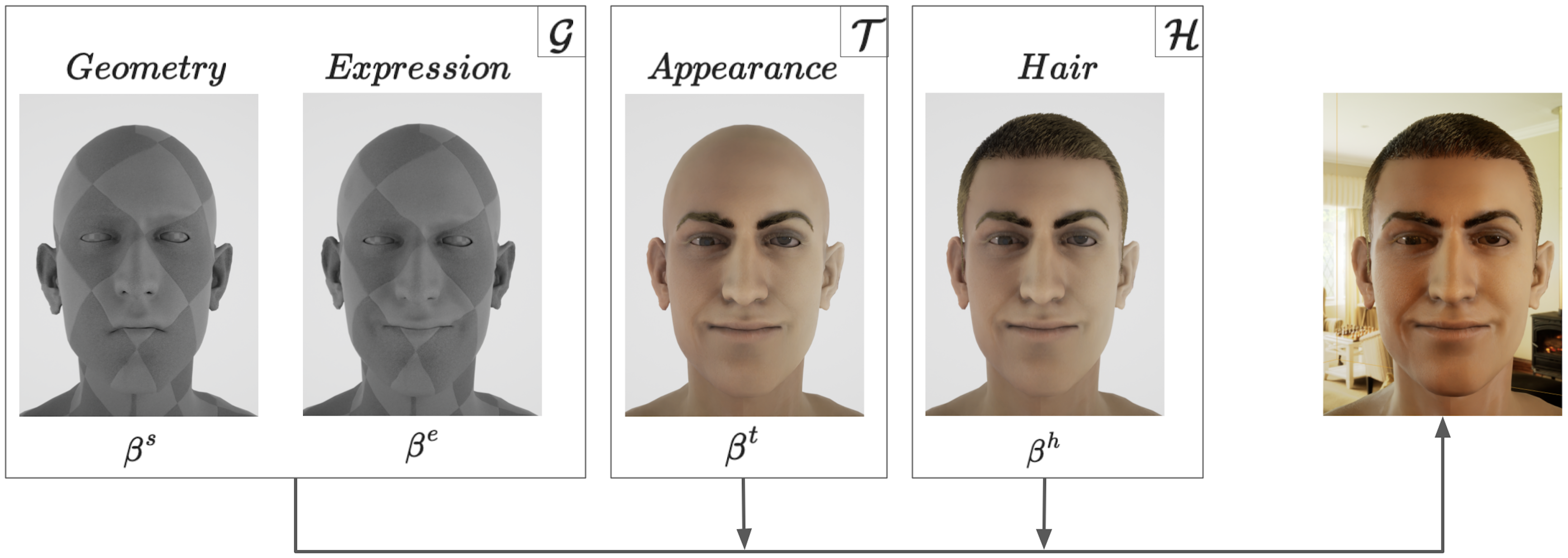
We introduce SPHEAR, a 3D articulated head model which contains generative shape, expression, hair, and appearance components, making it the first complete statistical head model to date. We start from an artist-defined rigged template mesh, where is the set of vertices and is the set of faces. The template has joints which also control the tongue, left and right eyeballs, and lower and upper eyelids. The initial set of skinning weights is . Formally, SPHEAR is controlled by a set of low-dimensional embedding vectors and pose parameters
The geometric component generates meshes with the same number of vertices and connectivity as the template. It is controlled using the shape encoding for the neutral expression, encodes facial expressions in neutral head pose, and is a vector containing the pose parameters and can be represented as Euler angles, rotation matrices, or 6D representations [95]. The appearance component generates high resolution color and normal textures from a latent representation . The hair component generates dense strands from a low-dimensional code.
To learn different model components, we collect a new 3D dataset of facial human expressions, FHE3D, containing 240K photorealistic scans captured from more than 600 diverse subjects with a proprietary system operating at 60Hz. For each subject, we capture 40 different facial expression tracks lasting 2 seconds each. For each scan, our system provides 3D geometry as well as texture maps. We keep a held out test set of 1,000 scans from 25 subjects, each with 40 different facial expressions (FHE3D-TEST).
In the sequel, we will describe the creation of SPHEAR, starting with the process of template registration to captured scans. We will then detail how we create the various components .
3.1 Sphere Embeddings for Accurate Registration
We call spherical embedding a diffeormorphism (i.e. invertible and smooth mapping) between the unit 2-sphere and any smooth 2-manifold of genus-0 , . The sphere is a strong regularizer to represent genus-0 topologies, and one can easily and efficiently parameterize them. For our use case, head meshes can be approximated as genus-0 topologies. We propose to reparameterize each training head scan as a sphere, by learning the mapping and its corresponding approximate inverse function . For all 3D points , then the functions have to satisfy . To regularize the solution, we discourage sharp changes in gradients by adding a penalty on the second-order derivatives of . This reparameterization can be used for shape learning, interpolation and for establishing semantically meaningful correspondences. We will apply these properties in the context of registration.
In contrast to our formulation, previous approaches enforce the invertibility property [34, 21, 55], either by using a family of bijective functions [55] or by integration over a smooth vector field [34, 21]. The invertibility property guarantees perfect reconstruction loss (because is bijective and ), but does not guarantee that the function is a bijection between the desired manifolds. The training loss is thus limited to either Chamfer distances or other indirect reconstruction losses, in order to force both manifolds to match the expected and . We argue that these approaches cannot capture the high-frequency details of head scans and limits potential applications where we would like to condition independently and . Please see Fig. 5 for an example.
Spherical registration.
Assuming we have a target scan , with arbitrary vertices and triangulation, we want to register the template to . This means explaining the geometry of the target by a deformation of the template in a semantically meaningful sense. This is an ill-posed problem, with many regularizations and procedures explored in the literature (ARAP [71], ACAP [89], etc.).
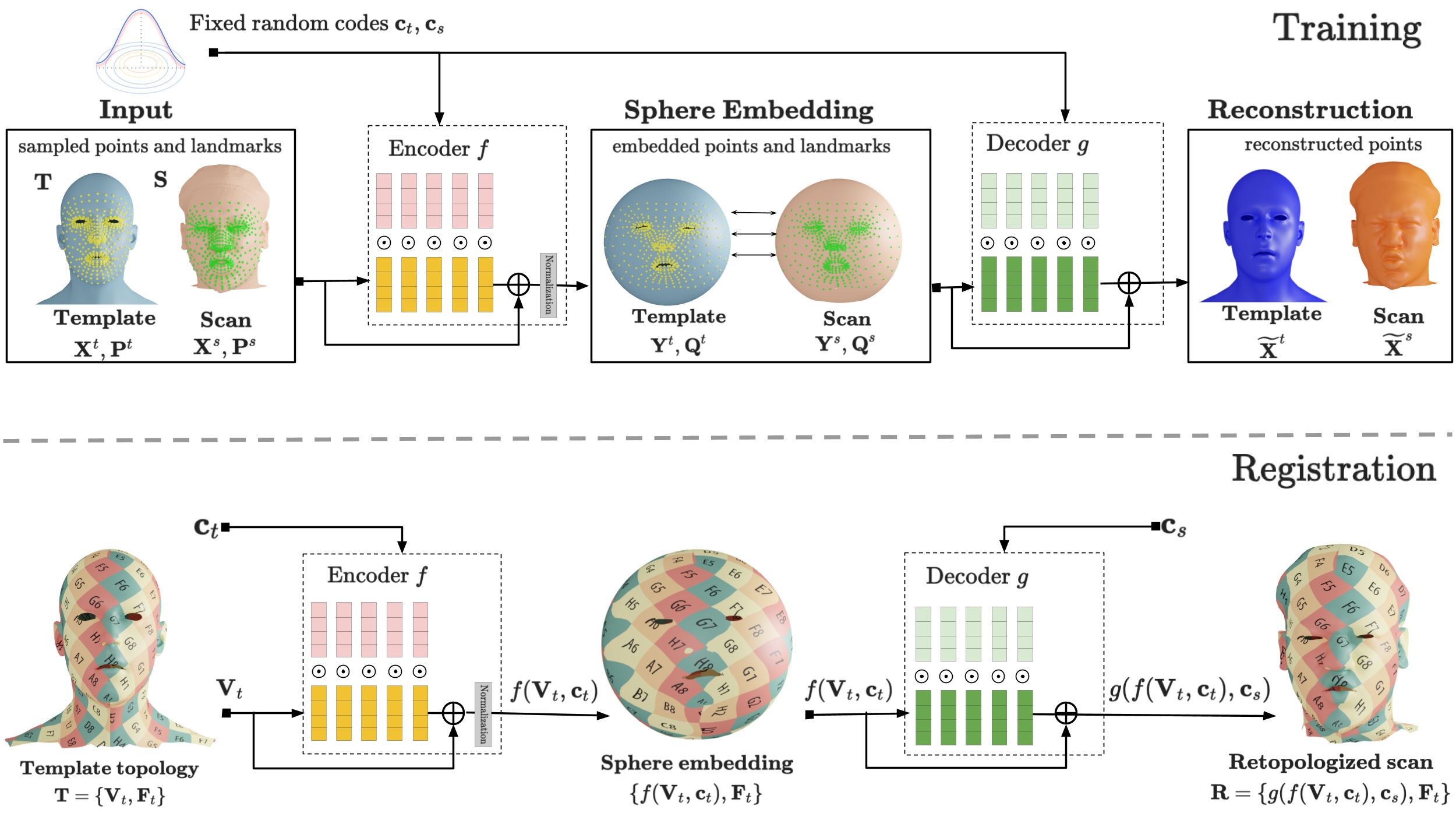
Our solution is to embed both the target and the template in the same spherical embedding space, where they must be aligned. To do so, we augment two Siren [70] activated MLPs, and with two additional modulator networks [50], . Here, is an input code to the modulation networks, while are trainable parameters. The codes will be used to modulate the Siren-based encoders and decoders, i.e. and . The encoder and decoder will have the following forms
| (1) | ||||
| (2) |
where is a normalization operator projecting all entries onto the unit 3D sphere. We remove explicit dependencies on for clarity.
For our task, we use randomly generated codes, and , for both the template and the target scan. During training, we will embed the template and the scan into the spherical space, through and , and decode them using and , respectively. To obtain aligned surfaces , at inference time, we will decode . For this to work, both mesh surfaces must be aligned in the spherical space. To enforce alignment, we use landmarks attached to each of the two meshes. We define for the scan landmarks and for the template, and guide them to be consistent in the spherical embedding spaces. In order to obtain we render in 16 synthetic views, with known camera parameters, and use FaceMesh [32] to obtain 478 2D landmarks . We triangulate these points (through nonlinear optimization) to obtain the desired 3D landmarks. For we use predefined semantic locations on the template .
To train our networks, we sample points on the scan surface – i.e. – and points on the surface of the template – i.e. – and reconstruct them using our encoder/decoder networks. The landmarks are embedded into the sphere and matched together. This amounts to the following losses
To ensure a smooth solution, we introduce a second-order regularization term, defined as the squared Frobenius norm of the Hessian matrix of , . We sample points on the surface of the sphere and then compute the regularization term
We add this regularization loss for both surfaces. The total loss becomes . Once trained, we can obtain the topology of either template or scan, but on the surface of the other. For example, to retrieve the template registered to the target scan, we simply compute
| (3) |
See Fig. 4 for a visual illustration of the method.
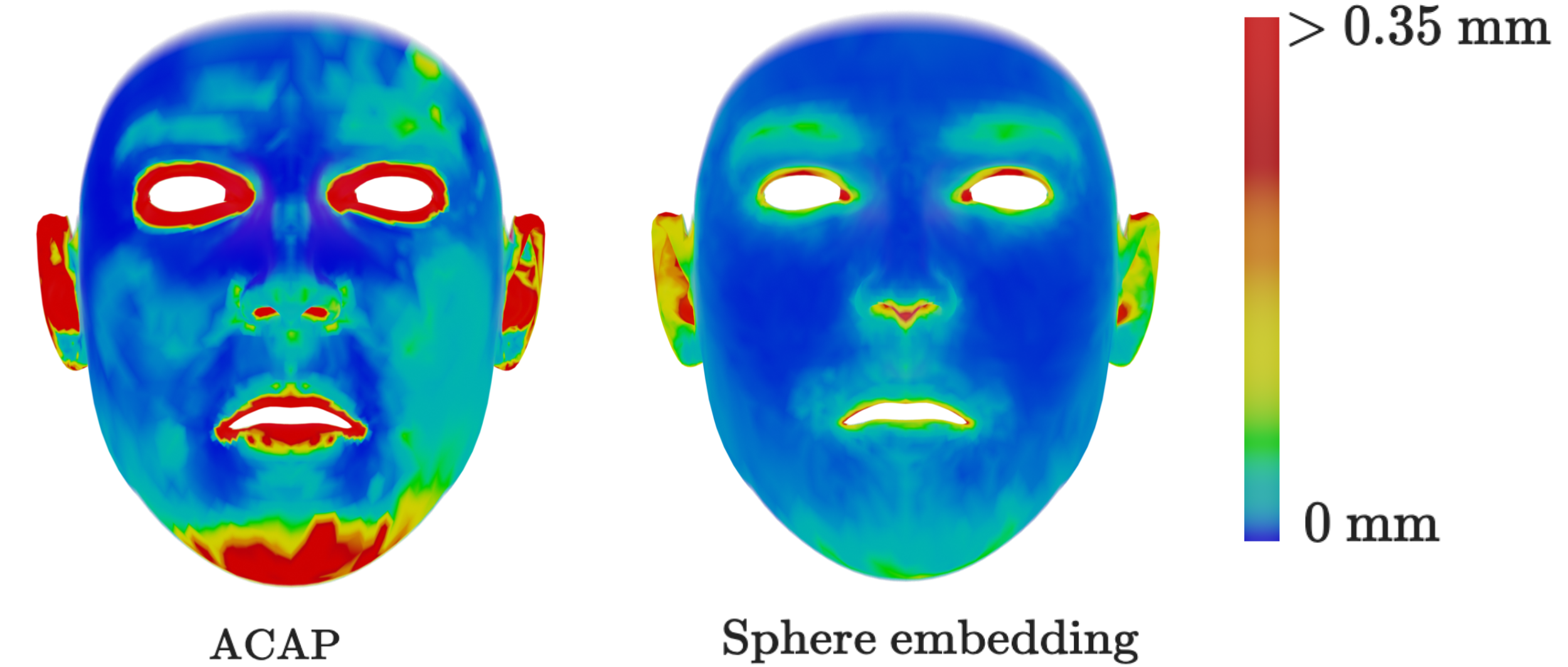
We train and test the registration pipeline, on the face region (including ears), against ACAP. We show averaged template-to-scan ICP error maps, across all training examples, in Fig. 8. The mean errors are mm for our method and mm for the classical ACAP registration. See the additional experiments in §4.
Tessellation invariant registration. Because our training pipeline maps points sampled on the surfaces, we are invariant to any particular tessellation of the input meshes. Our approach allows the registration of more detailed meshes to the target scan as long as these are aligned to the same level set as the original input template. Thus we can get new registrations of higher resolution meshes with only one feedforward pass through our spherical embedding encoders and decoders. For illustration, see Fig. 7, where we show how a subdivided template is used instead. Note that we do not require any new retraining, which makes the registration pipeline flexible to any new tessellation, vertex or face re-orderings.
Code semantics.
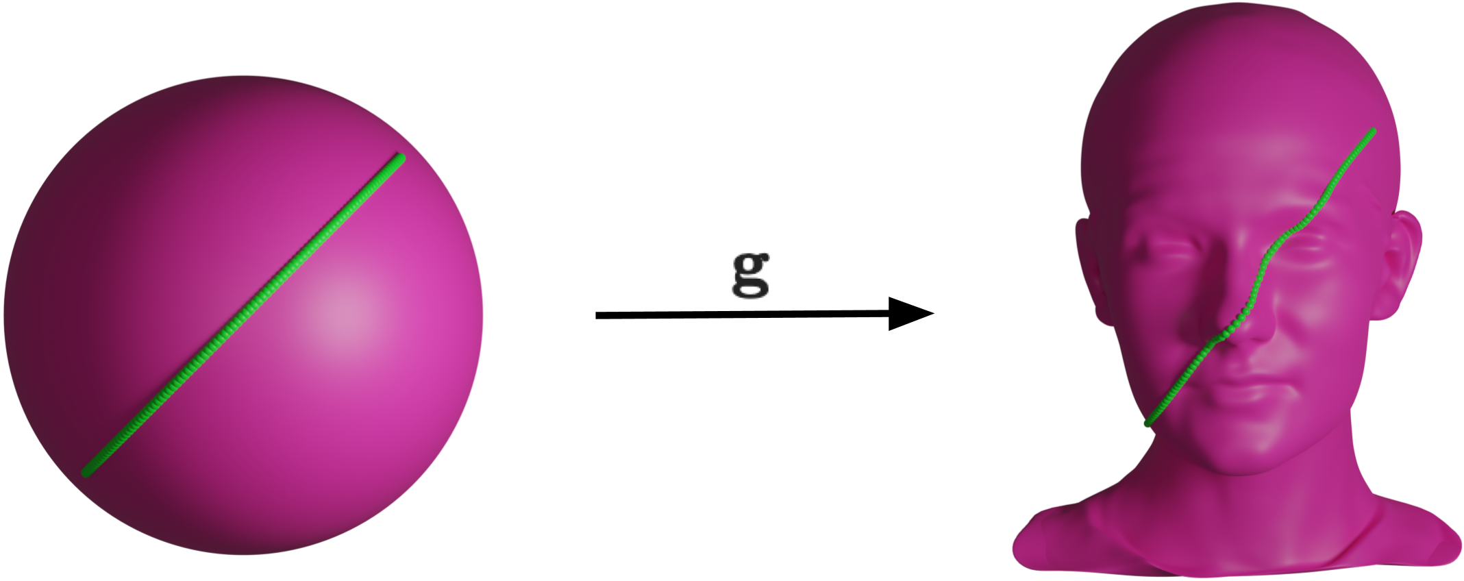
We do another experiment in which, instead of a template and a scan , we use two scans and , with associated latent codes and . To investigate the semantic meaning of these codes, we replicate the registration design for these new inputs. We then embed the vertices of into the sphere by , but decode by , where is an interpolation timestep between and . We show the interpolation result in Fig. 6. Notice how the reconstruction is a smooth transition from one scan to the other, while maintaining semantical knowledge about different face parts.

Secondary components.
Secondary components, such as eyes and teeth, are only partially captured by the scanner. The eyeballs are initialized using the triangulated positions of the iris landmarks [32]. Their position is further optimized so that we minimize eyeball intersections with the rest of the scan for all expressions of a given subject. We perform a similar operation for the position of the teeth. More detail is given in the Sup. Mat.
3.2 Generative Shape and Expression Model
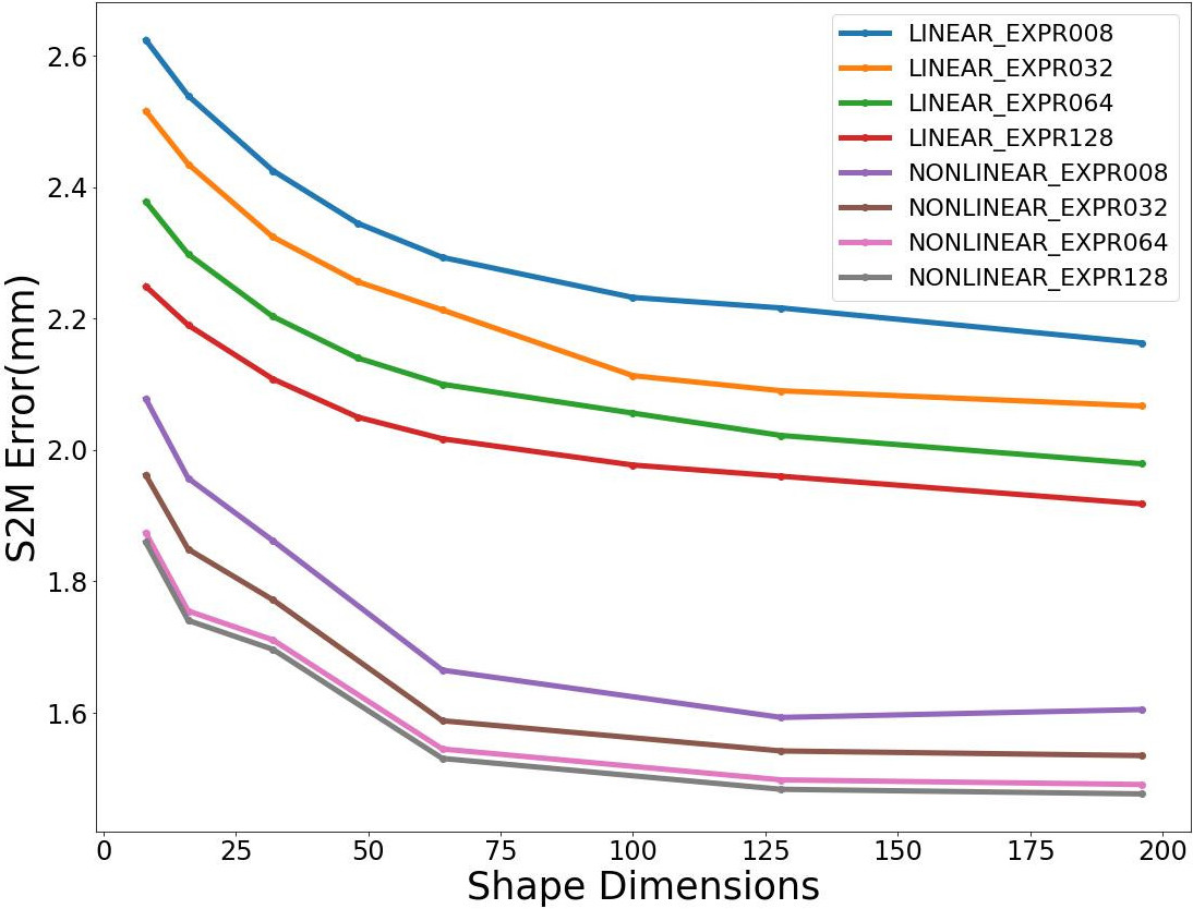
We employ the proposed spherical registration pipeline to register the template mesh on the FHE3D dataset. Additionally, we enhance the shape diversity by incorporating data from the CAESAR [63] dataset, which comprises 4,329 subjects annotated with facial landmarks. Following the approach in [85], we train an end-to-end head model that includes a shape embedding , a facial expression embedding , skinning weights , a shape-dependent joint centers regressor, and pose-space deformations, which depend on the head pose . The geometric model and its main sub-components are illustrated in Fig. 3. Both the shape and expression embeddings are modeled using a variational auto-encoder. The former is trained on disarticulated neutral shapes, while the latter is trained on disarticulated shapes with different expressions. We conduct an ablation study in Fig. 13, where we analyze the effects of varying the number of latent dimensions for the two embeddings, and additionally compare against a linear version based on PCA. We report the scan to mesh (S2M) fitting errors on the FHE3D-TEST set. We observe that errors saturate around dimensions and that further increasing embedding size brings little to no improvement. As a result, we also use dimensions for our embeddings in practice. Furthermore, the non-linear models show significant lower errors than the linear counterparts, validating our approach.

3.3 Generative Hair Model
To train our hair generation module , we use a collection of roughly hairstyles [38] with an average of hair strands, each with 3D coordinates of the control points. Our goal is to build a latent, generative space from which we can draw hair samples that are diverse, smooth, and intersection-free with the head mesh. We aim for generation speed, memory and back-propagation efficiency for fitting to different input modalities.
For each training sample, we represent its hair strands as a texture map for the scalp, where is the number of control points starting from the root, and is the resolution of the scalp texture. In practice, each hair strand is encoded in its tangent-bitangent-normal representation with respect to the starting triangle on the scalp. To improve memory requirements, we approximate the hair strands with parametric curves modeled as degree Legendre polynomials with ortho-normal bases. We obtain a new representation , where is the number of coefficients per polynomial. To build a generative space, we use variational auto-decoders [62, 53] where each training sample will have a trainable mean and log-variance , where is the latent embedding size. Using the re-parameterization trick [45] we get a code , where is sampled from . We use -divergence during training as a regularizer. For the network architecture, we use a similar approach to [40], where every code embedding will create an initial map, gradually de-convoluted to match the target hair texture. See the Sup. Mat. for more details on the network architecture and representation.
Properties
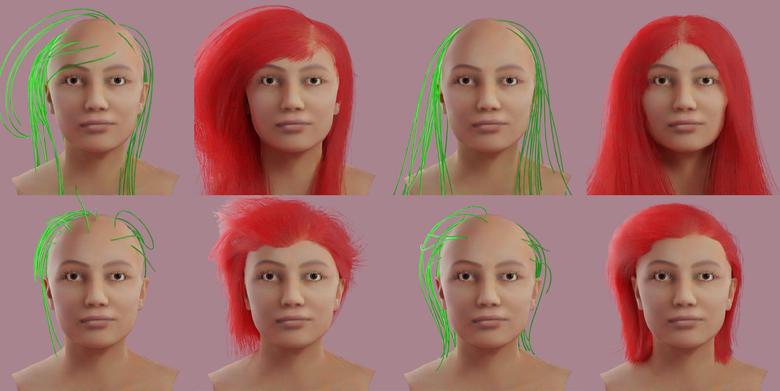
After training, we generate samples running , where is sampled from a standard normal distribution. In Fig. 10, we show that the learned latent space has semantics, by interpolating between randomly generated codes and showing the reconstructed hair. Because our method generates hair in a texture space, we can resize the maps to control the desired number of strands. Because the strands are encoded using Legendre polynomial bases, we can evaluate for any number of control points. This gives us flexibility in generating plausible hair styles for various computational budgets. Different from [65], which learns a latent space for each strand independently, we train a generative model for all our strands at once, basically being able to generate consistent hairstyles, not hair-strands. We also do not use Siren networks or modulators, or VAEs. Compared to variational volume encoding networks such as [68, 92], which are more involved and more accurate, we are much faster during inference: those methods decode in roughly second, while we do it in roughly - milliseconds. To show the practical application of our decoder architecture, we ran fitting experiments to various hair guides using BFGS. An experiment finished in under seconds, which amounts to network forward + backward passes. Results can be seen in Fig. 9.

3.4 Generative Appearance Model
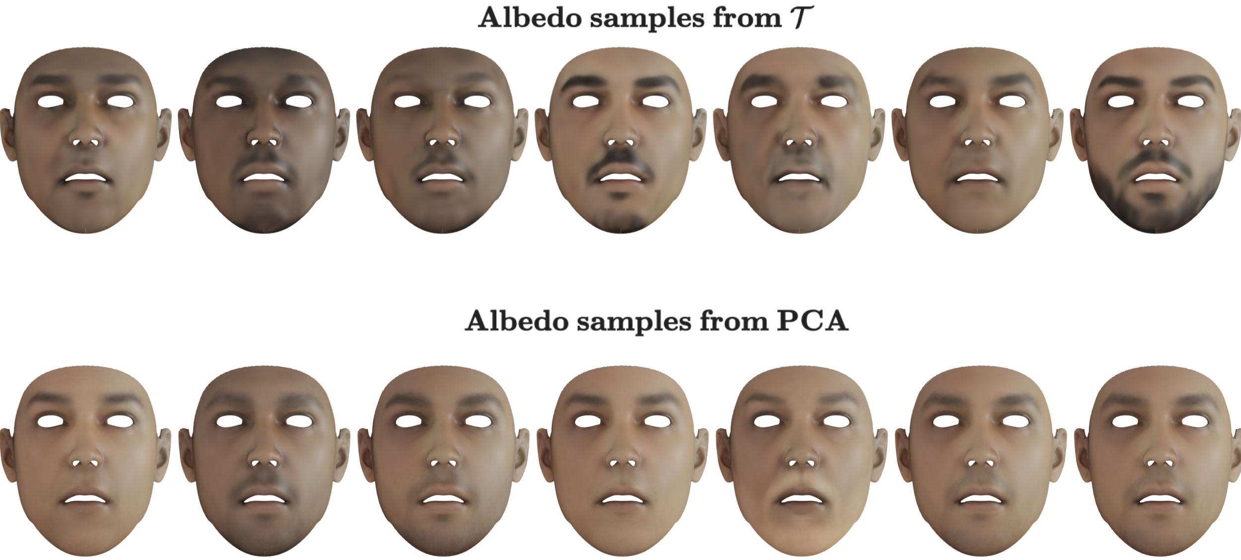
For completeness, we also train a generative face appearance model, similar in architecture to the hair network. To make it lighter, we downsample the target maps to resolution. At test time, we sample , where is the latent embedding size, from the standard normal distribution and obtain . We post-process by up-sampling using the super-resolution algorithm of [82] in order to obtain maps. We supervise training using an Euclidean distance loss between the ground truth and predicted maps. We also fit a PCA model with components to the training data and run comparisons to our proposed generator. On the training set, PCA has a mean absolute error (MAE) of , while our VAD-based solution achieves MAE. In Fig. 12, we qualitatively compare the two solutions for sampling quality, noticing that our method produces more detailed and diverse samples.
4 Additional Experiments
In this section we introduce additional experiments for registration, and 3D and 2D fitting, further evaluating the accuracy of our proposed spherical registration as well as SPHEAR’s accuracy, generalization capabilities, and fairness.
Registration.
We compare our spherical embedding registration with other state-of-the-art registration methods in Tab. 2. Our method achieves a improvement compared to [89]. We observed that both the deformation transfer [72] and the non-rigid ICP method from [5] are very sensitive to initialization. To achieve competitive results for the other methods, we first aligned the template scan using Procrustes analysis based on landmarks. For [89] we used our own implementation of ACAP, while for DT [72] and [5] we used the publicly available one [23].
| Method | Neutral (mm) | Expressions (mm) |
|---|---|---|
| DT [72] | 0.79 0.23 | 0.90 0.62 |
| NR-ICP [5] | 0.94 0.24 | 1.17 0.31 |
| ACAP [89] | 0.45 0.15 | 0.51 0.24 |
| SR (Ours) | 0.14 0.03 | 0.22 0.15 |
3D fitting.
We evaluate SPHEAR’s generalization to unseen identities with different facial expressions by fitting it against test scans from FHE3D-TEST. We compare SPHEAR on this task with state-of-the-art head models and report results in Tab. 3. For FLAME [48] and Facescape [86] we used the publicly available fitting code. For GHUM [85] we used the standalone head model. We used the same triangulated landmarks for all models obtained. We report average scan-to-mesh (S2M) errors of the face region on both scans in rest pose with neutral expression and for those featuring facial expressions. SPHEAR is the most accurate model and is the most reliable (together with GHUM), with the lowest error variation.
2D fitting and fairness evaluation.
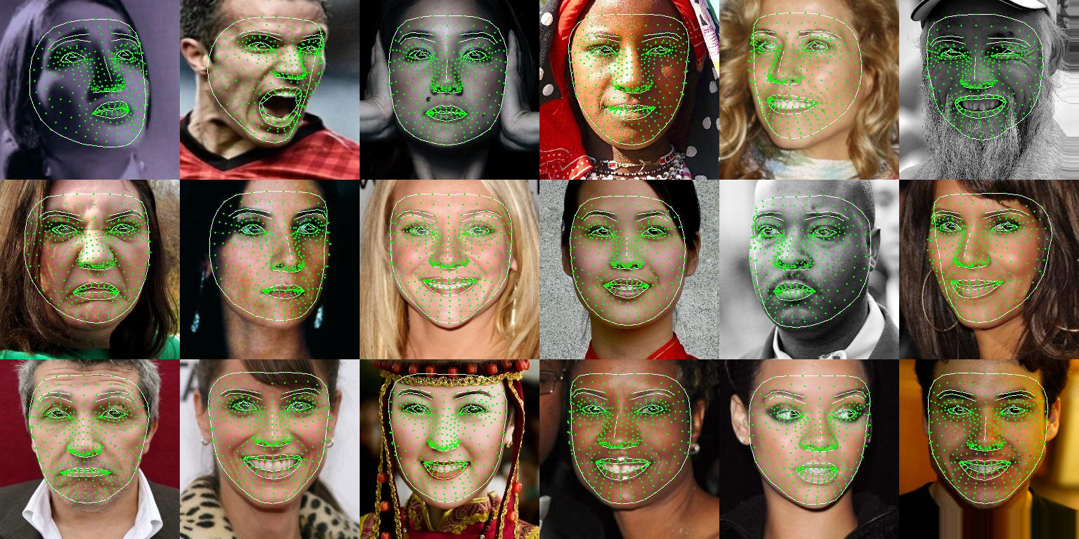
We evaluate SPHEAR’s accuracy and diversity via fitting to 2D landmarks. For this task, we utilize a dataset containing 1.7k images of people evenly distributed across 17 geographical subregions. Each image is annotated with 468 2D landmarks corresponding to the Facemesh [32] semantics and with a skin tone using the Fitzpatrick scale [1]. The 468 landmarks capture important variation in facial features and proportions across humanity. To this end, we use those as a reference for evaluating the accuracy and fairness of our model. We fit SPHEAR to each image using the 2D landmark reprojection error and analyze the remaining 2D fitting error in pixels for each skin tone group separately, see Tab. 4. Our model achieves the lowest errors across all head models and, more importantly, has consistent accuracy across all skin tones.
| Method | Neutral (mm) | Expressions (mm) |
|---|---|---|
| Facescape [86] | 1.59 0.66 | 1.60 0.31 |
| FLAME [48] | 1.58 0.62 | 1.77 0.39 |
| GHUM [85] | 1.44 0.24 | 1.63 0.31 |
| SPHEAR (Ours) | 1.36 0.28 | 1.58 0.30 |
| Method |
ST1
![[Uncaptioned image]](/html/2311.02461/assets/figures/fitzscale/fsc1.png)
|
ST2
![[Uncaptioned image]](/html/2311.02461/assets/figures/fitzscale/fsc2.png)
|
ST3
![[Uncaptioned image]](/html/2311.02461/assets/figures/fitzscale/fsc3.png)
|
ST4
![[Uncaptioned image]](/html/2311.02461/assets/figures/fitzscale/fsc4.png)
|
ST5
![[Uncaptioned image]](/html/2311.02461/assets/figures/fitzscale/fsc5.png)
|
ST6
![[Uncaptioned image]](/html/2311.02461/assets/figures/fitzscale/fsc6.png)
|
|---|---|---|---|---|---|---|
| Facescape [86] | 3.5 | 3.6 | 3.8 | 3.0 | 4.1 | 3.2 |
| FLAME [48] | 2.3 | 2.1 | 2.2 | 2.2 | 2.4 | 2.5 |
| GHUM [85] | 2.2 | 2.0 | 2.1 | 2.1 | 2.3 | 2.5 |
| SPHEAR | 1.7 | 1.7 | 1.7 | 1.7 | 1.7 | 1.8 |
5 Conclusions
To support a high degree of realism, we have developed a novel 3D registration methodology based on spherical embeddings, which benefits the construction of an accurate statistical 3D human head model. For completeness, we present additional components that enable fine-grained control in sampling diverse head shapes, facial expressions, skin appearance, and hair styles represented as strands. Experiments support the validity of design choices and the accuracy of our registration, reconstruction, and component generation techniques.
Ethical Considerations. Our methodology aims to decrease bias by supporting representation diversity and the generation of fair synthetic data. It facilitates bootstrapping for new domains and diverse subject distributions, where labeled data is often difficult to collect upfront. Our model is not intended or appropriate for any form of deep fakes. To faithfully represent a person with our model, we would need access to high-quality 3D scans, which requires explicit user consent. Although our model can be animated and realistically rendered, there may still be a gap between our renderings and real video.
Limitations: While our statistical model is the first of its kind, is still far from being perfect: we can do more in terms of modeling hair diversity (e.g. curliness), build more accurate normal/color reconstructions from raw scans, model micro-details, muscle and fat tissues. Learning more detailed statistical components for partially hidden structures, e.g. teeth or the skull, may require additional imagery including CT scans.
Supplementary Material
In this supplementary material, we give examples of additional applications of our proposed spherical embedding, detail the hair and appearance networks, provide additional experiments, and showcase SPHEAR’s diversity.
Appendix A Spherical geometry applications
The spherical embedding we propose for registration has interesting applications beyond registration, as we show in the sequel. Concretely, we demonstrate how we can improve 3D landmark triangulation and how one can interpolate between two scans using the same methodology.
A.1 Landmark triangulation
3D landmark triangulation.
One key prerequisite in learning and is the high fidelity registration of the template head mesh to the training set of scans. The first step in the registration process is to detect a set of semantically consistent 3D landmarks on each scan. For scalable, automatic and accurate head registration, we use FaceMesh [32] to obtain 478 2D landmarks, in 16 synthetic views , with known camera parameters. We triangulate these points (through nonlinear optimization) to obtain the desired 3D landmarks.
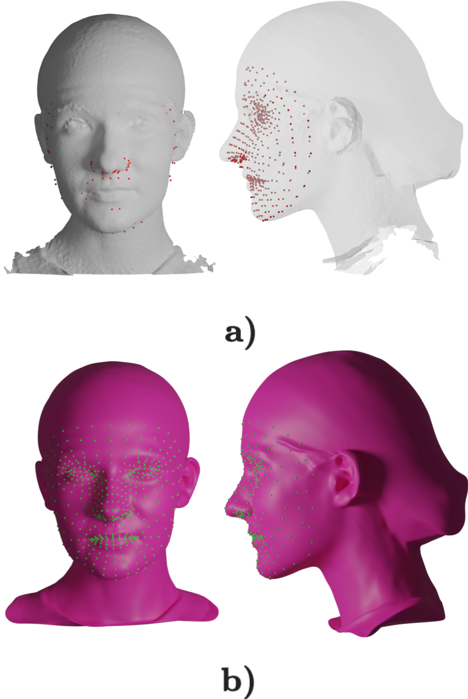
One issue with triangulated 3D landmarks from 2D detections is that they ignore the 3D geometry of the scan. Errors in 2D landmark inference will translate into errors in surface positioning. For example, the landmark for the tip of the nose might “sink” way below the nose surface, see Fig. 14 a). We would like to constrain the 3D landmarks to remain on the surface during triangulation. We use our proposed spherical embedding, modeled as a trainable mapping with Siren activation networks [70].
Similarly to Sec. 3.1 in the main paper, let be a point on the scan surface, and let be the point on the unit sphere, where is a trainable ‘encoder‘ network. To decode, we compute , where is the corresponding, trainable ‘decoder‘ network. Both networks are based on Siren activated MLPs,
| (4) | ||||
| (5) |
where are the trainable parameters of and , respectively, and is the unit-sphere projection. In the following paragraph, we will drop the explicit dependency for clarity.
For a given scan we sample points on its surface, , and compute the reconstruction loss
| (6) |
To ensure a smooth solution, we use as defined in Eq. 5, from the main paper.
The final loss is then , where is the weight given to the regularization term, which depends on the global training step (it decreases in log space from to ).
After training the sphere embedding, we define a non-linear optimization problem that starts from the solution of the classical triangulation routine, , but in sphere space, i.e. , and uses the perspective operator which projects the decoded landmarks in all camera views
| (7) |
After convergence, we retrieve the solution . This guarantees that reconstructed landmarks stay on the surface of the sphere and, implicitly, on the surface of the scan.
In Fig. 14 a), we present the originally triangulated points , from 16 different camera views. Notice how the points “sink” below the surface, failing to capture the nose and lips completely. Constraining the landmarks to sit on the surface of the scan, results in much better localization – see Fig. 14 b). The scan in Fig. 14 b) is actually the result of the learned network , when applied to an icosphere of depth 7, with vertices and triangular faces. The scan embedding error was, in this case, mm.
Architecture design choices.
We experimented with different options for our network architectures (i.e. ). We use a collection of scans , for which we compute their reconstruction error for all vertices as defined by in Eq. 6. We also compute a per-vertex normal error, between the original vertex normals and the transformed vertex normals of . In Tab. 5, we show ablation results. First ablation, “w MLPs”, uses ReLU activated MLPs instead of Siren-based MLPs. The second one, “w MLPs and RFE”, adds a Random Fourier Embedding [73] to the 3D points, before processing by the MLPs. This means constructing a kernel matrix , with entries drawn from . The scale is assigned through validation. The RFE embeddings will be . Both architectures performed worse than our model, in terms of both errors, while also displaying some artifacts.
| Method | Reconstr. Error (mm) | Normal Error (°) |
|---|---|---|
| w MLPs | ||
| w MLPs and RFE | ||
| Ours |
A.2 Registration
Implementation details.
We set the modulation codes, , to be 3-dimensional, and we initialize them from a truncated standard normal distribution. We did not observe improved performance with a larger code size. For the Siren networks and Siren modulators, we use 5 intermediate layers with 128 hidden neurons, for a total of k and k parameters, respectively. Note that we change the intermediate activation to tanh for the Siren modulators, as ReLU was failing to converge. The networks are trained for 10000 steps, with 512 sampled points each iteration (on the scan surfaces), and 256 sampled points on the sphere. The whole training takes roughly minutes on a Nvidia Titan XP graphics card. The main bottleneck is the second-order Hessian computation (through which we have to pass gradients), for the regularizer .
Appendix B Hair network
Texture space embedding.
We embed each hair strand , where is the number of control points of the curve, in the UV texture space of the template scalp. To facilitate training, we also parameterize in the TBN (tangent, bitangent and normal) space, such that the variance across directions is reduced [65]. We also observed that by encoding them by relative offsets improves performance – i.e. .
Legendre polynomial bases.
We observe that training a network directly for generating control points, leads to very spiky, non-smooth results. To address this issue, we turn towards expressing the hair strands as parameterized curves. We choose to use Legendre polynomials. They form a system of orthogonal polynomials , defined over the interval , such that:
| (8) |
We fit a 5-th degree polynomial with Legendre bases (which we call Legendre polynomial), i.e. , to all hair strands, for each Cartesian component separately. The weights will uniquely describe each hair strand, and we get . To make sure that distances between polynomials make sense, we have to ensure that the orthogonal polynomial bases are also ortho-normal. For that, we compute the norm of each of basis and divide by it:
| (9) |
Note that only by having Legendre polynomials (or other described by ortho-normal bases) ensures that distances between curves are proportional to distances between samples on the curves.
Limitations.
Note that a polynomial with degree can have at most turning points. This is a limiting factor in modeling more complex hair strands, with a lot of curliness. We chose the degree to , as the dataset on which we train does not exhibit curly hair. However, we can control curliness after generation, with some post-processing, if needed.
Network details.
We take a variational auto-decoder approach [90, 35], and assign a unique identifier to each training example. The network, similar to [40], goes from a code an initial map () , and to a final map through sequential deconvolutions and upsampling blocks. Like in [41], we also replace the nearest-neighbour upsampling with bilinear sampling. The complete network has trainable parameters and is trained with Adam optimizer [44], batch size of , learning rate of and a decay of .
Intersection-free penalty.
Once trained, samples might, qualitatively, look smooth and plausible, but they will not necessarily respect physical constraints: i.e. they might intersect with the head template. In order to address this, we revisit the training procedure. We embed the head template into a sphere (similar to A.1), and re-attach the hair training samples. We re-parameterize the strands in terms of , where and ., where is the control point. This is basically expressing any control point in terms of spherical coordinates plus a non-negative scaling factor, which guarantees that any control point is not inside the sphere, and, implicitly, not inside the head.
Appendix C Appearance network
Normal generation.
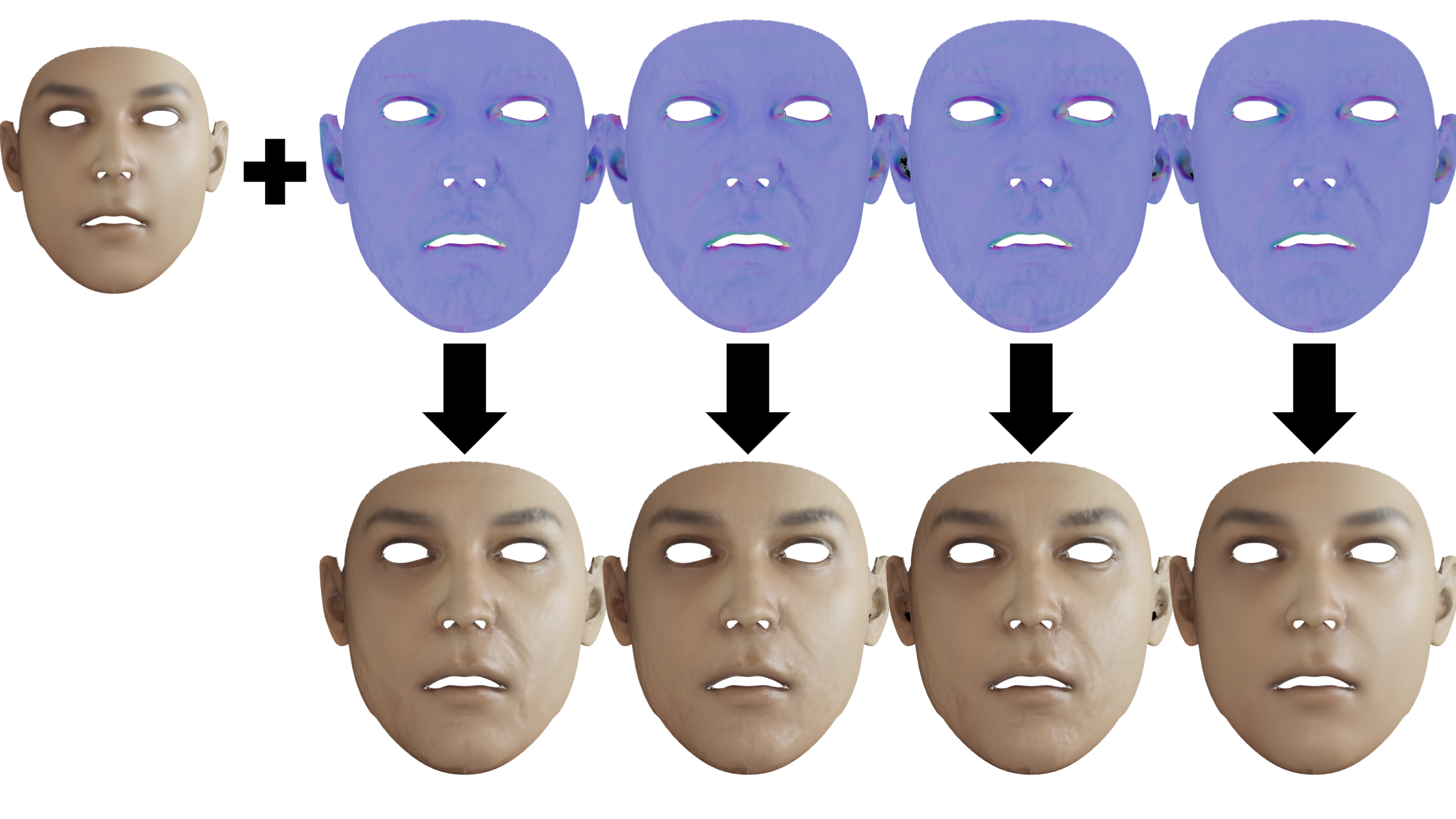
We also show the quality of sampled normals, from our appearance generator , in Fig. 16. Normals are important for increasing the visual fidelity of the renderings, and it is a cheap way of encoding skin imperfections, wrinkles or geometric deformations.
Network details.
We use a very similar architecture to the hair network, but we make changes to the number of processing layers, as the final map is times as big, from to . Note that in practice, we have 2 generative appearance models, one for albedo and for normals. Each of them has roughly trainable parameters.
Appendix D Diversity
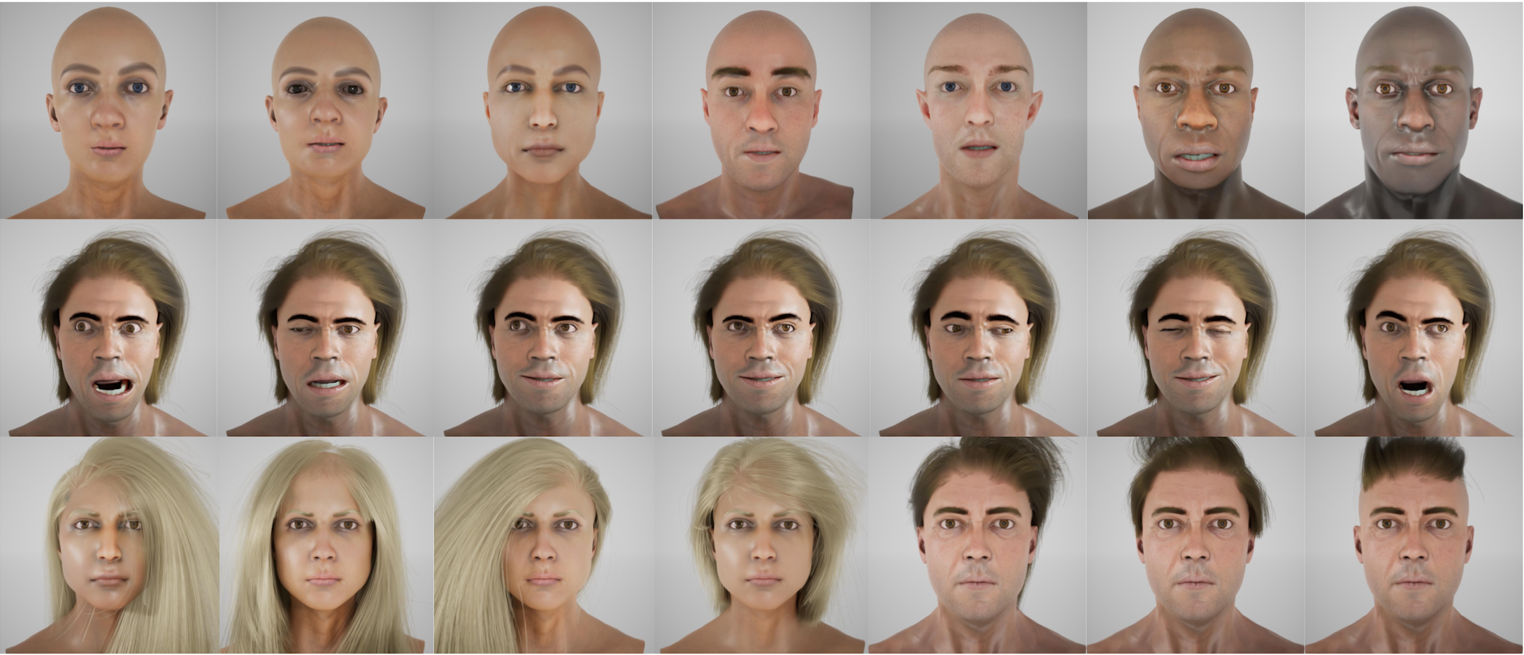
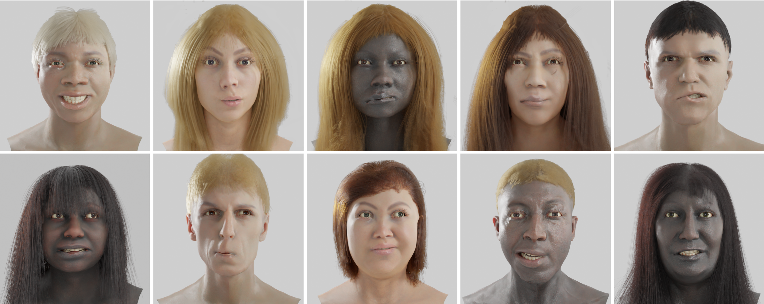
To show that our samples lead to fair machine learning algorithms, we report the distributions of various attributes for the scan data used in training our generators. We consider the skin color distribution of our captured subjects in our FHE3D dataset, covering different ethnicities, the body mass index and the age (see Fig. 17). As it can be observed, the distribution is fairly weighted across all considered brackets.Once trained, SPHEAR allows us to sample diverse 3D heads of people with varying identity, expression, eye gaze, and hair style, see Fig. 15.
Teeth Texture Variation.
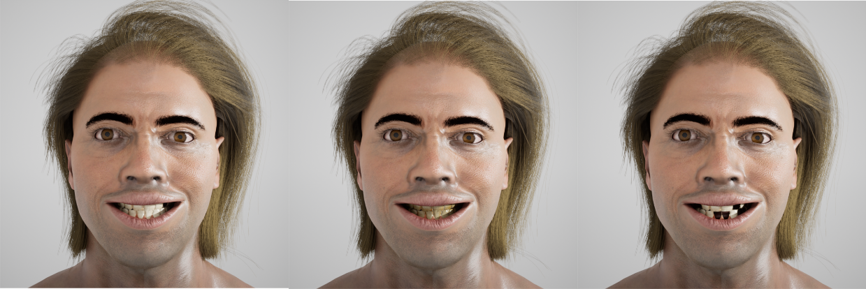
Capturing teeth geometry for teeth is difficult given the current systems. We rely instead on a procedural method to control erosion effects, teeth discoloration, presence of cavities and lack of teeth. We implement the effects as a material shader compatible with existing photorealistic rendering engines. We illustrate such examples in Fig. 18.
Appendix E Applications
In the sequel we demonstrate three different applications of SPHEAR. First, we represent 3D head scans with SPHEAR through fitting. Next, we provide additional results for the 2D fitting experiment from the main paper. Finally, we use SPHEAR for synthetic data generation for two different tasks: 2D landmark detection and dense semantic labeling. Using SPHEAR, obtaining accurate labels is cheap and we show that trained predictors generalize well to real images.
3D Fitting.
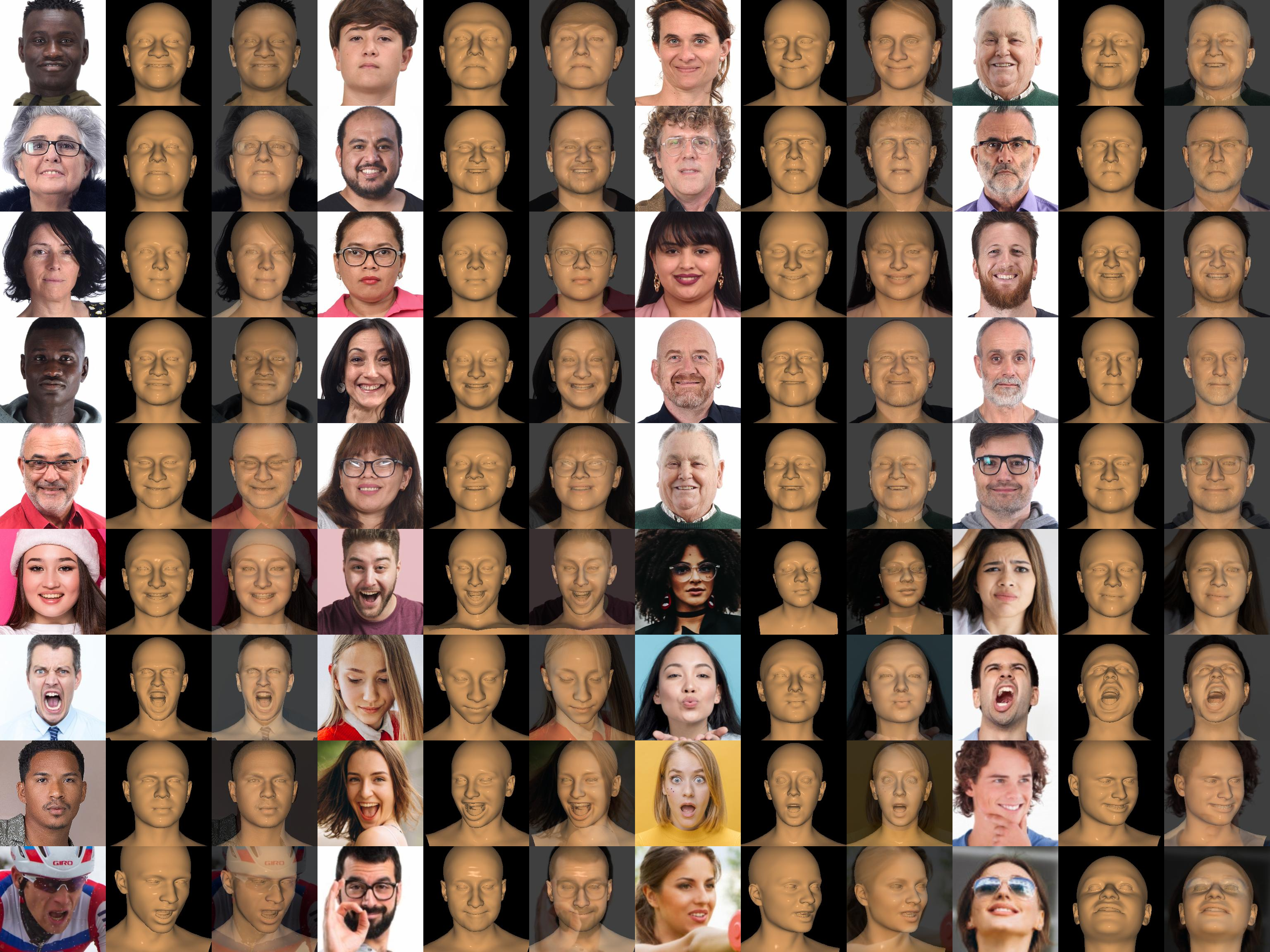
Given a textured 3D scan geometry of the head of a person, we are interested in fitting the parameters of our geometric component , . The SPHEAR mesh vertex positions are then given by this geometric component . Similar to the registration pipeline, we use FaceMesh [32] to obtain 2D landmarks, in 16 different rendered views of the scan. We triangulate these points (through nonlinear optimization) and refine them using the sphere embedding approach (cf. Sec. A.1). We denote the final 3D landmarks on the scan surface as . We then optimize the head model parameters with respect to (1) the alignment to the 3D landmarks, together with (2) an implicit ICP-type loss driven by the learned spherical embedding. The optimization loss can be written as:
where is a sparse matrix used to regress the landmarks locations from the SPHEAR vertices and are scalars used to weigh the two terms. In the second term, represents the reconstruction of the vertices through the sphere embedding of the scan. This guarantees that these reconstructed points are on the scan surface. This acts similar in spirit to ICP, where one instead of using would consider the nearest-neighbors of on the scan. Compared to classical ICP, where the process of finding the nearest point at each optimization step is non-differentiable, our objective is fully differentiable, is faster to compute and leads to smaller errors (mesh-to-scan average distances, in mm): vs on neutral shapes, and vs on shapes with expressions.
2D Fitting.
We provide more examples of our 2D fitting results in figure Fig. 21. As illustrated by the experiments in the main paper our model fits well to diverse identities, facial expressions and head poses.
| Method | Common | Challenging | Private |
|---|---|---|---|
| Real | 3.33 | 5.59 | 4.53 |
| Synthetic | 3.52 | 6.62 | 4.91 |
Landmark Predictions.
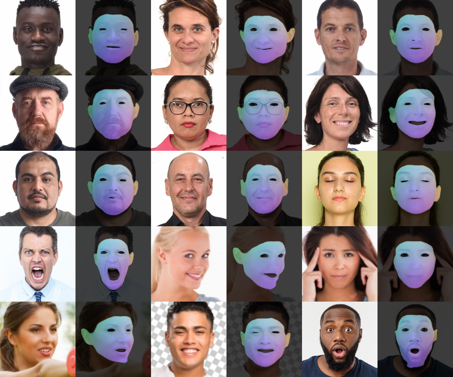
We evaluate the usefulness of our SPHEAR model in a 2D landmark detection task. For this, we generate a synthetic dataset of rendered faces from various viewpoints, with sampled attributes from , a discrete set of eye colors and HDRI backgrounds. In total, we generate 60K samples for training and 10K samples for validation using 500 HDRI images from the public domain [36]. These allow us to vary illumination patterns and backgrounds. We trained a lightweight real-time production-level face mesh network (1M parameters) [32] to predict 478 dense landmarks using purely synthetic supervision. In Fig. 20, we show that our trained model generalizes to unseen images in-the-wild. For quantitative evaluation, we trained a similar real-time network on an in-house dataset, consisting of 20K real images with manually annotated landmarks. We test both methods on the public 300W dataset [66]. For both networks, we also trained an additional two-layer domain adaptation network to regress the landmarks that are annotated in 300W. We report results in Tab. 6 and observe on par performance. Overall, this reduces the need for costly annotations, as is often the case when using manually labeled data, while maintaining comparable performance.
Dense Predictions.
Besides the landmarks estimation application we also explored a dense semantic prediction task. For the each synthetic data example generated using SPHEAR, we rendered a semantic mask of the ground truth head geometry containing the 3D template coordinates as attributes. We also considered rasterizing the UV coordinate attributes instead, however the UV coordinates are not continuous especially close to the texture seams[9, 3]. We then trained a UNet[64] network , taking as input RGB images, in order to predict rasterized semantic masks. For each coordinate in the output mask, the dense correspondence network predicts a 3D coordinate on the SPHEAR template. We present some sample qualitative results in Fig. 20.
References
- [1] https://en.wikipedia.org/wiki/Fitzpatrick_scale.
- Abrevaya et al. [2018] Victoria Fernández Abrevaya, Stefanie Wuhrer, and Edmond Boyer. Multilinear autoencoder for 3d face model learning. In Winter Conf. on Applications of Computer Vision, pages 1–9. IEEE, 2018.
- Alldieck et al. [2021] Thiemo Alldieck, Hongyi Xu, and Cristian Sminchisescu. imghum: Implicit generative models of 3d human shape and articulated pose. In Proceedings of the IEEE/CVF International Conference on Computer Vision, pages 5461–5470, 2021.
- Alldieck et al. [2022] Thiemo Alldieck, Mihai Zanfir, and Cristian Sminchisescu. Photorealistic monocular 3d reconstruction of humans wearing clothing. In Proceedings of the IEEE/CVF Conference on Computer Vision and Pattern Recognition (CVPR), 2022.
- Amberg et al. [2007] Brian Amberg, Sami Romdhani, and Thomas Vetter. Optimal step nonrigid icp algorithms for surface registration. In 2007 IEEE conference on computer vision and pattern recognition, pages 1–8. IEEE, 2007.
- Athar et al. [2022] ShahRukh Athar, Zexiang Xu, Kalyan Sunkavalli, Eli Shechtman, and Zhixin Shu. Rignerf: Fully controllable neural 3d portraits. In CVPR, pages 20364–20373, 2022.
- Bagautdinov et al. [2018] Timur Bagautdinov, Chenglei Wu, Jason Saragih, Pascal Fua, and Yaser Sheikh. Modeling facial geometry using compositional vaes. In Proceedings of the IEEE Conference on Computer Vision and Pattern Recognition, pages 3877–3886, 2018.
- Bazavan et al. [2021] Eduard Gabriel Bazavan, Andrei Zanfir, Mihai Zanfir, William T Freeman, Rahul Sukthankar, and Cristian Sminchisescu. Hspace: Synthetic parametric humans animated in complex environments. arXiv preprint arXiv:2112.12867, 2021.
- Bhatnagar et al. [2020] Bharat Lal Bhatnagar, Cristian Sminchisescu, Christian Theobalt, and Gerard Pons-Moll. Loopreg: Self-supervised learning of implicit surface correspondences, pose and shape for 3d human mesh registration. Advances in Neural Information Processing Systems, 33:12909–12922, 2020.
- Blanz and Vetter [2002] Volker Blanz and Thomas Vetter. A morphable model for the synthesis of 3d faces. SIGGRAPH’99 Proceedings of the 26th annual conference on Computer graphics and interactive techniques, 2002.
- Bolkart and Wuhrer [2015] Timo Bolkart and Stefanie Wuhrer. A groupwise multilinear correspondence optimization for 3D faces. In Proceedings of the IEEE International Conference on Computer Vision (ICCV), pages 3604–3612, 2015.
- Booth et al. [2016a] James Booth, Anastasios Roussos, Stefanos Zafeiriou, Allan Ponniah, and David Dunaway. A 3d morphable model learnt from 10,000 faces. In Proceedings of the IEEE Conference on Computer Vision and Pattern Recognition (CVPR), 2016a.
- Booth et al. [2016b] James Booth, Anastasios Roussos, Stefanos Zafeiriou, Allan Ponniah, and David Dunaway. A 3d morphable model learnt from 10,000 faces. In CVPR, pages 5543–5552, 2016b.
- Booth et al. [2017] James Booth, Epameinondas Antonakos, Stylianos Ploumpis, George Trigeorgis, Yannis Panagakis, and Stefanos Zafeiriou. 3d face morphable models ”in-the-wild”. In CVPR, 2017.
- Booth et al. [2018] James Booth, Anastasios Roussos, Allan Ponniah, David Dunaway, and Stefanos Zafeiriou. Large scale 3d morphable models. 126(2):233–254, 2018.
- Burkov et al. [2022] Egor Burkov, Ruslan Rakhimov, Aleksandr Safin, Evgeny Burnaev, and Victor Lempitsky. Multi-neus: 3d head portraits from single image with neural implicit functions. arXiv preprint arXiv:2209.04436, 2022.
- Cao et al. [2013] Chen Cao, Yanlin Weng, Shun Zhou, Yiying Tong, and Kun Zhou. Facewarehouse: A 3d facial expression database for visual computing. IEEE Transactions on Visualization and Computer Graphics, 20(3):413–425, 2013.
- Chen et al. [2018] Ricky T. Q. Chen, Yulia Rubanova, Jesse Bettencourt, and David K Duvenaud. Neural ordinary differential equations. In Advances in Neural Information Processing Systems. Curran Associates, Inc., 2018.
- Cheng et al. [2021a] An-Chieh Cheng, Xueting Li, Min Sun, Ming-Hsuan Yang, and Sifei Liu. Learning 3d dense correspondence via canonical point autoencoder. Advances in Neural Information Processing Systems, 34:6608–6620, 2021a.
- Cheng et al. [2022] An-Chieh Cheng, Xueting Li, Sifei Liu, Min Sun, and Ming-Hsuan Yang. Autoregressive 3d shape generation via canonical mapping. In European Conference on Computer Vision, pages 89–104. Springer, 2022.
- Cheng et al. [2021b] Ziang Cheng, Hongdong Li, Richard I. Hartley, Yinqiang Zheng, and Imari Sato. One ring to rule them all: a simple solution to multi-view 3d-reconstruction of shapes with unknown BRDF via a small recurrent resnet. CoRR, abs/2104.05014, 2021b.
- Corona et al. [2023] Enric Corona, Mihai Zanfir, Thiemo Alldieck, Eduard Gabriel Bazavan, Andrei Zanfir, and Cristian Sminchisescu. Structured 3d features for reconstructing relightable and animatable avatars. In CVPR, 2023.
- [23] Dawson-Haggerty et al. trimesh.
- Deng et al. [2022] Bailin Deng, Yuxin Yao, Roberto M Dyke, and Juyong Zhang. A survey of non-rigid 3d registration. In Computer Graphics Forum, pages 559–589. Wiley Online Library, 2022.
- Dinh et al. [2016] Laurent Dinh, Jascha Sohl-Dickstein, and Samy Bengio. Density estimation using real nvp. arXiv preprint arXiv:1605.08803, 2016.
- Egger et al. [2019] Bernhard Egger, William A. P. Smith, Ayush Tewari, Stefanie Wuhrer, Michael Zollhoefer, Thabo Beeler, Florian Bernard, Timo Bolkart, Adam Kortylewski, Sami Romdhani, Christian Theobalt, Volker Blanz, and Thomas Vetter. 3d morphable face models – past, present and future, 2019.
- Feng et al. [2021] Yao Feng, Haiwen Feng, Michael J. Black, and Timo Bolkart. Learning an animatable detailed 3D face model from in-the-wild images. ACM Transactions on Graphics (ToG), Proc. SIGGRAPH, 40(4):88:1–88:13, 2021.
- Gafni et al. [2021] Guy Gafni, Justus Thies, Michael Zollhoefer, and Matthias Nießner. Dynamic neural radiance fields for monocular 4d facial avatar reconstruction. In CVPR, 2021.
- Gerig et al. [2018] Thomas Gerig, Andreas Morel-Forster, Clemens Blumer, Bernhard Egger, Marcel Luthi, Sandro Schönborn, and Thomas Vetter. Morphable face models-an open framework. In Int. Conf. on Automatic Face & Gesture Recognition, pages 75–82. IEEE, 2018.
- Giebenhain et al. [2023] Simon Giebenhain, Tobias Kirschstein, Markos Georgopoulos, Martin Rünz, Lourdes Agapito, and Matthias Nießner. Learning neural parametric head models. In CVPR, 2023.
- Goodfellow et al. [2014] Ian Goodfellow, Jean Pouget-Abadie, Mehdi Mirza, Bing Xu, David Warde-Farley, Sherjil Ozair, Aaron Courville, and Yoshua Bengio. Generative adversarial nets. In NIPS, 2014.
- Grishchenko et al. [2020] Ivan Grishchenko, Artsiom Ablavatski, Yury Kartynnik, Karthik Raveendran, and Matthias Grundmann. Attention mesh: High-fidelity face mesh prediction in real-time. arXiv preprint arXiv:2006.10962, 2020.
- Groueix et al. [2018] Thibault Groueix, Matthew Fisher, Vladimir G Kim, Bryan C Russell, and Mathieu Aubry. 3d-coded: 3d correspondences by deep deformation. In Proceedings of the european conference on computer vision (ECCV), pages 230–246, 2018.
- Gupta and Chandraker [2020] Kunal Gupta and Manmohan Chandraker. Neural mesh flow: 3d manifold mesh generationvia diffeomorphic flows, 2020.
- Hao et al. [2020] Zekun Hao, Hadar Averbuch-Elor, Noah Snavely, and Serge Belongie. Dualsdf: Semantic shape manipulation using a two-level representation. In Proceedings of the IEEE/CVF Conference on Computer Vision and Pattern Recognition, pages 7631–7641, 2020.
- [36] Poly Haven. Poly haven: The public 3d asset library.
- Hong et al. [2022] Yang Hong, Bo Peng, Haiyao Xiao, Ligang Liu, and Juyong Zhang. Headnerf: A real-time nerf-based parametric head model. In Proceedings of the IEEE/CVF Conference on Computer Vision and Pattern Recognition, pages 20374–20384, 2022.
- Hu et al. [2015] Liwen Hu, Chongyang Ma, Linjie Luo, and Hao Li. Single-view hair modeling using a hairstyle database. ACM Transactions on Graphics (ToG), 34(4):1–9, 2015.
- Huang et al. [2020] Zeng Huang, Yuanlu Xu, Christoph Lassner, Hao Li, and Tony Tung. Arch: Animatable reconstruction of clothed humans. In IEEE/CVF Conference on Computer Vision and Pattern Recognition (CVPR), 2020.
- Karras et al. [2017] Tero Karras, Timo Aila, Samuli Laine, and Jaakko Lehtinen. Progressive growing of gans for improved quality, stability, and variation. arXiv preprint arXiv:1710.10196, 2017.
- Karras et al. [2019] Tero Karras, Samuli Laine, and Timo Aila. A style-based generator architecture for generative adversarial networks. In Proceedings of the IEEE/CVF conference on computer vision and pattern recognition, pages 4401–4410, 2019.
- Kemelmacher-Shlizerman [2013] Ira Kemelmacher-Shlizerman. Internet based morphable model. In 2013 IEEE International Conference on Computer Vision, pages 3256–3263, 2013.
- Khakhulin et al. [2022] Taras Khakhulin, Vanessa Sklyarova, Victor Lempitsky, and Egor Zakharov. Realistic one-shot mesh-based head avatars. In ECCV, 2022.
- Kingma and Ba [2014] Diederik P Kingma and Jimmy Ba. Adam: A method for stochastic optimization. arXiv preprint arXiv:1412.6980, 2014.
- Kingma and Welling [2013] Diederik P Kingma and Max Welling. Auto-encoding variational bayes. arXiv preprint arXiv:1312.6114, 2013.
- Li et al. [2020a] Jiaman Li, Zhengfei Kuang, Yajie Zhao, Mingming He, Kalle Bladin, and Hao Li. Dynamic facial asset and rig generation from a single scan. ACM Transactions on Graphics, 39:1–18, 2020a.
- Li et al. [2020b] Ruilong Li, Karl Bladin, Yajie Zhao, Chinmay Chinara, Owen Ingraham, Pengda Xiang, Xinglei Ren, Pratusha Prasad, Bipin Kishore, Jun Xing, et al. Learning formation of physically-based face attributes. In Proceedings of the IEEE/CVF conference on computer vision and pattern recognition, pages 3410–3419, 2020b.
- Li et al. [2017] Tianye Li, Timo Bolkart, Michael J Black, Hao Li, and Javier Romero. Learning a model of facial shape and expression from 4d scans. ACM Trans. Gr., 36(6):194–1, 2017.
- Luo et al. [2021] Huiwen Luo, Koki Nagano, Han-Wei Kung, Qingguo Xu, Zejian Wang, Lingyu Wei, Liwen Hu, and Hao Li. Normalized avatar synthesis using stylegan and perceptual refinement. In Proceedings of the IEEE/CVF Conference on Computer Vision and Pattern Recognition (CVPR), pages 11662–11672, 2021.
- Mehta et al. [2021] Ishit Mehta, Michaël Gharbi, Connelly Barnes, Eli Shechtman, Ravi Ramamoorthi, and Manmohan Chandraker. Modulated periodic activations for generalizable local functional representations. In Proceedings of the IEEE/CVF International Conference on Computer Vision, pages 14214–14223, 2021.
- Mihajlovic et al. [2022] Marko Mihajlovic, Aayush Bansal, Michael Zollhoefer, Siyu Tang, and Shunsuke Saito. KeypointNeRF: Generalizing image-based volumetric avatars using relative spatial encoding of keypoints. In European conference on computer vision, 2022.
- Olszewski et al. [2020] Kyle Olszewski, Duygu Ceylan, Jun Xing, Jose Echevarria, Zhili Chen, Weikai Chen, and Hao Li. Intuitive, interactive beard and hair synthesis with generative models. In IEEE/CVF Conference on Computer Vision and Pattern Recognition (CVPR), 2020.
- Park et al. [2019] Jeong Joon Park, Peter Florence, Julian Straub, Richard Newcombe, and Steven Lovegrove. Deepsdf: Learning continuous signed distance functions for shape representation. In Proceedings of the IEEE/CVF conference on computer vision and pattern recognition, pages 165–174, 2019.
- Park et al. [2021] Keunhong Park, Utkarsh Sinha, Jonathan T. Barron, Sofien Bouaziz, Dan B Goldman, Steven M. Seitz, and Ricardo Martin-Brualla. Nerfies: Deformable neural radiance fields. ICCV, 2021.
- Paschalidou et al. [2021] Despoina Paschalidou, Angelos Katharopoulos, Andreas Geiger, and Sanja Fidler. Neural parts: Learning expressive 3d shape abstractions with invertible neural networks. In Proceedings of the IEEE/CVF Conference on Computer Vision and Pattern Recognition, pages 3204–3215, 2021.
- Paysan et al. [2009] Pascal Paysan, Reinhard Knothe, Brian Amberg, Sami Romdhani, and Thomas Vetter. A 3d face model for pose and illumination invariant face recognition. In 2009 sixth IEEE international conference on advanced video and signal based surveillance, pages 296–301. Ieee, 2009.
- Ploumpis et al. [2019] Stylianos Ploumpis, Haoyang Wang, Nick Pears, William AP Smith, and Stefanos Zafeiriou. Combining 3d morphable models: A large scale face-and-head model. In Proceedings of the IEEE/CVF Conference on Computer Vision and Pattern Recognition, pages 10934–10943, 2019.
- Ploumpis et al. [2020] Stylianos Ploumpis, Evangelos Ververas, Eimear O’Sullivan, Stylianos Moschoglou, Haoyang Wang, Nick Pears, William Smith, Baris Gecer, and Stefanos P Zafeiriou. Towards a complete 3d morphable model of the human head. 2020.
- Qiu et al. [2022] Zesong Qiu, Yuwei Li, Dongming He, Qixuan Zhang, Longwen Zhang, Yinghao Zhang, Jingya Wang, Lan Xu, Xudong Wang, Yuyao Zhang, et al. Sculptor: Skeleton-consistent face creation using a learned parametric generator. arXiv preprint arXiv:2209.06423, 2022.
- Ramon et al. [2021] Eduard Ramon, Gil Triginer, Janna Escur, Albert Pumarola, Jaime Garcia, Xavier Giro-i Nieto, and Francesc Moreno-Noguer. H3D-Net: Few-shot high-fidelity 3d head reconstruction. In Proceedings of the IEEE/CVF International Conference on Computer Vision, pages 5620–5629, 2021.
- Ranjan et al. [2018] Anurag Ranjan, Timo Bolkart, Soubhik Sanyal, and Michael J Black. Generating 3d faces using convolutional mesh autoencoders. In Proceedings of the European conference on computer vision (ECCV), pages 704–720, 2018.
- Rezende and Mohamed [2015] Danilo Jimenez Rezende and Shakir Mohamed. Variational inference with normalizing flows. arXiv preprint arXiv:1505.05770, 2015.
- Robinette et al. [2002] Kathleen M Robinette, Sherri Blackwell, Hein Daanen, Mark Boehmer, and Scott Fleming. Civilian american and european surface anthropometry resource (caesar), final report. volume 1. summary. Technical report, Sytronics Inc Dayton Oh, 2002.
- Ronneberger et al. [2015] Olaf Ronneberger, Philipp Fischer, and Thomas Brox. U-net: Convolutional networks for biomedical image segmentation. In International Conference on Medical image computing and computer-assisted intervention, pages 234–241. Springer, 2015.
- Rosu et al. [2022] Radu Alexandru Rosu, Shunsuke Saito, Ziyan Wang, Chenglei Wu, Sven Behnke, and Giljoo Nam. Neural strands: Learning hair geometry and appearance from multi-view images. ECCV, 2022.
- Sagonas et al. [2016] Christos Sagonas, Epameinondas Antonakos, Georgios Tzimiropoulos, Stefanos Zafeiriou, and Maja Pantic. 300 faces in-the-wild challenge: Database and results. Image and vision computing, 47:3–18, 2016.
- Saito et al. [2018] Shunsuke Saito, Liwen Hu, Chongyang Ma, Hikaru Ibayashi, Linjie Luo, and Hao Li. 3d hair synthesis using volumetric variational autoencoders. In SIGGRAPH Asia 2018 Technical Papers, pages 208:1–208:12, New York, NY, USA, 2018. ACM.
- Saito et al. [2019] Shunsuke Saito, Zeng Huang, Ryota Natsume, Shigeo Morishima, Angjoo Kanazawa, and Hao Li. Pifu: Pixel-aligned implicit function for high-resolution clothed human digitization. In Proceedings of the IEEE/CVF International Conference on Computer Vision (ICCV), 2019.
- Sanyal et al. [2019] Soubhik Sanyal, Timo Bolkart, Haiwen Feng, and Michael J Black. Learning to regress 3d face shape and expression from an image without 3d supervision. In Proceedings of the IEEE/CVF Conference on Computer Vision and Pattern Recognition, pages 7763–7772, 2019.
- Sitzmann et al. [2020] Vincent Sitzmann, Julien Martel, Alexander Bergman, David Lindell, and Gordon Wetzstein. Implicit neural representations with periodic activation functions. Advances in Neural Information Processing Systems, 33:7462–7473, 2020.
- Sorkine and Alexa [2007] Olga Sorkine and Marc Alexa. As-rigid-as-possible surface modeling. In Symposium on Geometry processing, pages 109–116, 2007.
- Sumner and Popović [2004] Robert W Sumner and Jovan Popović. Deformation transfer for triangle meshes. ACM Transactions on graphics (TOG), 23(3):399–405, 2004.
- Tancik et al. [2020] Matthew Tancik, Pratul Srinivasan, Ben Mildenhall, Sara Fridovich-Keil, Nithin Raghavan, Utkarsh Singhal, Ravi Ramamoorthi, Jonathan Barron, and Ren Ng. Fourier features let networks learn high frequency functions in low dimensional domains. pages 7537–7547, 2020.
- Taylor et al. [2012] Jonathan Taylor, Jamie Shotton, Toby Sharp, and Andrew Fitzgibbon. The vitruvian manifold: Inferring dense correspondences for one-shot human pose estimation. In 2012 IEEE Conference on Computer Vision and Pattern Recognition, pages 103–110. IEEE, 2012.
- Tewari et al. [2020] Ayush Tewari, Mohamed Elgharib, Gaurav Bharaj, Florian Bernard, Hans-Peter Seidel, Patrick Pérez, Michael Zollhofer, and Christian Theobalt. Stylerig: Rigging stylegan for 3d control over portrait images. In CVPR, pages 6142–6151, 2020.
- Thies et al. [2020] Justus Thies, Mohamed Elgharib, Ayush Tewari, Christian Theobalt, and Matthias Nießner. Neural voice puppetry: Audio-driven facial reenactment. In ECCV, pages 716–731. Springer, 2020.
- Tran and Liu [2018] Luan Tran and Xiaoming Liu. Nonlinear 3d face morphable model. In IEEE Computer Vision and Pattern Recognition (CVPR), Salt Lake City, UT, 2018.
- Tran and Liu [2019] Luan Tran and Xiaoming Liu. On learning 3d face morphable model from in-the-wild images. IEEE Transactions on Pattern Analysis and Machine Intelligence, 2019.
- Tran et al. [2019] Luan Tran, Feng Liu, and Xiaoming Liu. Towards high-fidelity nonlinear 3d face morphable model. In In Proceeding of IEEE Computer Vision and Pattern Recognition, Long Beach, CA, 2019.
- Vlasic et al. [2006] Daniel Vlasic, Matthew Brand, Hanspeter Pfister, and Jovan Popovic. Face transfer with multilinear models. In ACM SIGGRAPH 2006 Courses, 2006.
- Wang et al. [2022] Daoye Wang, Prashanth Chandran, Gaspard Zoss, Derek Bradley, and Paulo Gotardo. Morf: Morphable radiance fields for multiview neural head modeling. In ACM SIGGRAPH 2022 Conference Proceedings, pages 1–9, 2022.
- Wang et al. [2018] Xintao Wang, Ke Yu, Shixiang Wu, Jinjin Gu, Yihao Liu, Chao Dong, Yu Qiao, and Chen Change Loy. Esrgan: Enhanced super-resolution generative adversarial networks. In Proceedings of the European conference on computer vision (ECCV) workshops, pages 0–0, 2018.
- Wood et al. [2021] Erroll Wood, Tadas Baltrušaitis, Charlie Hewitt, Sebastian Dziadzio, Thomas J. Cashman, and Jamie Shotton. Fake it till you make it: Face analysis in the wild using synthetic data alone. In Proceedings of the IEEE/CVF International Conference on Computer Vision (ICCV), pages 3681–3691, 2021.
- Xie et al. [2022] Yiheng Xie, Towaki Takikawa, Shunsuke Saito, Or Litany, Shiqin Yan, Numair Khan, Federico Tombari, James Tompkin, Vincent Sitzmann, and Srinath Sridhar. Neural fields in visual computing and beyond. pages 641–676, 2022.
- Xu et al. [2020] Hongyi Xu, Eduard Gabriel Bazavan, Andrei Zanfir, Bill Freeman, Rahul Sukthankar, and Cristian Sminchisescu. GHUM & GHUML: Generative 3D human shape and articulated pose models. CVPR, 2020.
- Yang et al. [2020] Haotian Yang, Hao Zhu, Yanru Wang, Mingkai Huang, Qiu Shen, Ruigang Yang, and Xun Cao. Facescape: a large-scale high quality 3d face dataset and detailed riggable 3d face prediction. In Proceedings of the ieee/cvf conference on computer vision and pattern recognition, pages 601–610, 2020.
- Yang et al. [2018] Yaoqing Yang, Chen Feng, Yiru Shen, and Dong Tian. Foldingnet: Point cloud auto-encoder via deep grid deformation. In Proceedings of the IEEE conference on computer vision and pattern recognition, pages 206–215, 2018.
- Yenamandra et al. [2021] Tarun Yenamandra, Ayush Tewari, Florian Bernard, Hans-Peter Seidel, Mohamed Elgharib, Daniel Cremers, and Christian Theobalt. i3dmm: Deep implicit 3d morphable model of human heads. In CVPR, pages 12803–12813, 2021.
- Yoshiyasu et al. [2014] Yusuke Yoshiyasu, Wan‐Chun Ma, Eiichi Yoshida, and Fumio Kanehiro. As-conformal-as-possible surface registration. Computer Graphics Forum, 2014.
- Zadeh et al. [2019] Amir Zadeh, Yao-Chong Lim, Paul Pu Liang, and Louis-Philippe Morency. Variational auto-decoder: A method for neural generative modeling from incomplete data. arXiv preprint arXiv:1903.00840, 2019.
- Zanfir et al. [2022] Mihai Zanfir, Thiemo Alldieck, and Cristian Sminchisescu. Phomoh: Implicit photorealistic 3d models of human heads. arXiv preprint arXiv:2212.07275, 2022.
- Zhang and Zheng [2019] Meng Zhang and Youyi Zheng. Hair-gan: Recovering 3d hair structure from a single image using generative adversarial networks. Visual Informatics, 3(2):102–112, 2019.
- Zheng et al. [2022a] Mingwu Zheng, Hongyu Yang, Di Huang, and Liming Chen. Imface: A nonlinear 3d morphable face model with implicit neural representations. In Proceedings of the IEEE/CVF Conference on Computer Vision and Pattern Recognition, pages 20343–20352, 2022a.
- Zheng et al. [2022b] Yufeng Zheng, Victoria Fernández Abrevaya, Marcel C. Bühler, Xu Chen, Michael J. Black, and Otmar Hilliges. I M Avatar: Implicit morphable head avatars from videos. In CVPR, 2022b.
- Zhou et al. [2018a] Yi Zhou, Connelly Barnes, Jingwan Lu, Jimei Yang, and Hao Li. On the continuity of rotation representations in neural networks. arXiv preprint arXiv:1812.07035, 2018a.
- Zhou et al. [2018b] Yi Zhou, Liwen Hu, Jun Xing, Weikai Chen, Han-Wei Kung, Xin Tong, and Hao Li. Hairnet: Single-view hair reconstruction using convolutional neural networks. In Computer Vision – ECCV 2018, pages 249–265, Cham, 2018b. Springer International Publishing.
- Zielonka et al. [2022] Wojciech Zielonka, Timo Bolkart, and Justus Thies. Towards metrical reconstruction of human faces. In European Conference on Computer Vision, 2022.