LISNeRF Mapping: LiDAR-based Implicit Mapping via Semantic Neural Fields for Large-Scale 3D Scenes

Abstract

Large-scale semantic mapping is crucial for outdoor autonomous agents to fulfill high-level tasks such as planning and navigation. This paper proposes a novel method for large-scale 3D semantic reconstruction through implicit representations from LiDAR measurements alone. We firstly leverages an octree-based and hierarchical structure to store implicit features, then these implicit features are decoded to semantic information and signed distance value through shallow Multilayer Perceptrons (MLPs). We adopt off-the-shelf algorithms to predict the semantic labels and instance IDs of point cloud. Then we jointly optimize the implicit features and MLPs parameters with self-supervision paradigm for point cloud geometry and pseudo-supervision pradigm for semantic and panoptic labels. Subsequently, Marching Cubes algorithm is exploited to subdivide and visualize the scenes in the inferring stage. For scenarios with memory constraints, a map stitching strategy is also developed to merge sub-maps into a complete map. As far as we know, our method is the first work to reconstruct semantic implicit scenes from LiDAR-only input. Experiments on three real-world datasets, SemanticKITTI, SemanticPOSS and nuScenes, demonstrate the effectiveness and efficiency of our framework compared to current state-of-the-art 3D mapping methods.

(a) Point Cloud Input	(b) Neural Geometric Mesh	(c) Ours (Neural Semantic)	(d) Ours (Neural Panoptic)

Figure 1: Our LISNeRF framework implicitly represents a semantic scene with LiDAR-only input. Different mapping results are shown above via evaluating on sequence 00 of SemanticKITTI. (a) is the raw LiDAR point cloud for input. (b) is the neural scene representation using an implicit method called SHINE_Mapping [1]. (c) and (d) are semantic and panoptic reconstruction results via our implicit mapping.

I INTRODUCTION

Mapping and localization in unknown environments is a key technology for autonomous driving and mobile robots. On the one hand, in certain complex environments like urban street areas, maps is a prerequisite for path planning, and semantic-enriched maps enable the feasibility of intelligent navigation. On the other hand, accurate 3D semantic reconstruction of scene facilitates the application of Virtual Reality (VR) and Augmented Reality (AR).

Most existing works of 3D semantic reconstruction [2] [3] [4] are developed for RGB-D cameras and indoor environments which are not suitable for large-scale outdoor environments. For large-scale mapping, LiDAR plays a crucial role due to its ability to provide accurate distance measurement. However, large-scale 3D dense reconstruction and semantic mapping based on LiDAR sensor remains challenging because of the sparsity of LiDAR point clouds and the huge size of outdoor environments.

Recently, Neural Radiance Fields (NeRF) [5] has shown promising results in implicitly reconstructing a scene via adopting a Multi-Layer Perceptron [6], [7], [8]. Those NeRF-based frameworks is able to achieve higher mapping quality in indoor environments with a RGB-D sensor. While, those indoor-oriented methods face challenges when they are extended to large-scale environments, due to sensor detection range and computation resources. SHINE_Mapping [1] creatively employs sparse grids to implicitly represent a large-scale urban scene based on the LiDAR data alone, but it only provides geometric modeling of the environment and lacks of semantic elements, which is indispensable for modern high-level autonomous tasks.

To this end, we propose a novel implicit LiDAR mapping framework to incorporate semantic elements into the dense map (See Fig. 1). Inspire by [1], we exploit sparse octree-based feature vectors to implicitly represent and store the semantic information. Those feature vectors are obtained by optimizing loss functions with self-supervision from point cloud, and pseudo-supervision from semantic segmentation or panoptic segmentation. Given the spatial location coordinates of an arbitrary point, the SDF is obtain through geometric neural fields (GNF) and semantic label is obtain through semantic neural field (SNF). For explicitly displaying the implicit scene, Marching Cubes algorithm is adopted to reconstruct a scene with the form of semantic mesh. Besides, semantic mapping paradigm is further extended to the panoptic mapping by stacking more MLPs.

In summary, our contributions are as follows:

• We propose, to the best of our knowledge, the first method to construct neural implicit semantic map for large-scale environment from LiDAR data alone.

• We also extend neural semantic mapping to neural panoptic mapping by leveraging off-the-shelf panoptic segmentation modules. Then triple MLPs are stacked into the mapping for regressing instance labels.

• We design a map concatenation strategy to merge submaps into a complete map, to cope with computation limit of on-board devices in large-scale mapping tasks.

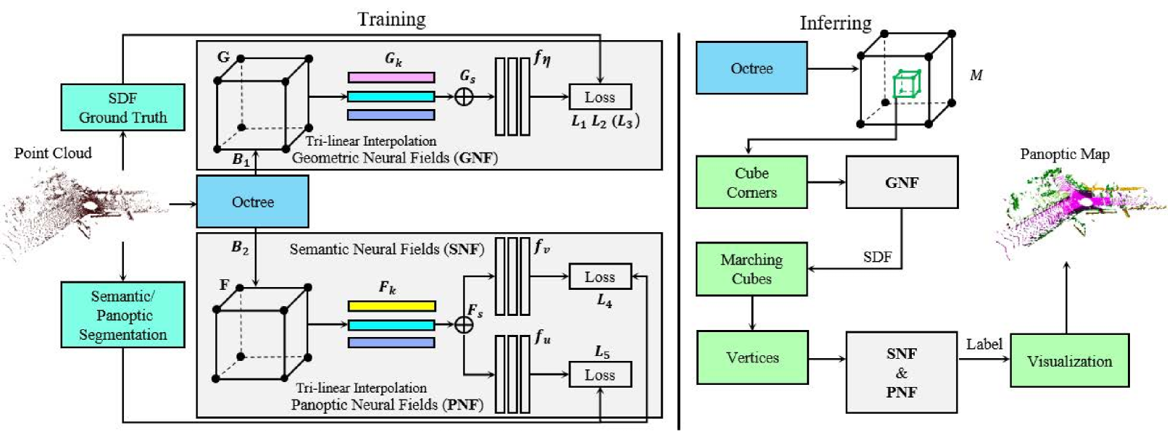
Figure 2: The overview of our LISNeRF framework. We firstly construct the Geometry Neural Fields (GNF), Semantic Neural Fields (SNF) and Panoptic Neural Fields (PNF) in the trainable feature vectors of octree and MLPs in the training procedure, then we calculate the current map size $M$ and predict the semantic lables of cube vertices in the inferring procedure. Given any arbitrary cube corner point in the map, we query the SDF valule through GNF. After obtaining the vertices using the Marching Cubes algorithm, we exploit SNF and PNF to query the their semantic labels. Specifically, semantic mapping obtain the semantic label using the entire feature vector through SNF. Panoptic mapping utilizes feature vectors with a certain proportion of length to regress the classes of ‘thing and stuff’ through PNF, and leverages other part of feature vectors to obtain instance ID of the ‘thing’ classes through PNF.

II RELATED WORK

Explicit mapping. Traditional 3D reconstruction represents a scene explicitly, and lots of map presentations are developed, such as point cloud (LeGO-LOAM [9], Loam_livox [10]), sufels (SuMa [11]), occupancy grids (Cartographer [12]), triangle meshes ( Puma [13], BnV-fusion [14]). Kimera [4] provides a semantic mapping method that only requires running on CPU. SuMa++ [15] extends SuMa [11] to semantic mapping, which is able to eliminate dynamic objects in the environment. However, the map built with sufels are relatively sparser compared to triangle mesh. Voxblox [16] utilizes Truncated Signed Distance Function (TSDF) to reconstruct a dense map in real-time. Voxblox++ [17] incorporates semantic information into Voxblox framework, but it only fits RGB-D sensor so that is infeasible for large-scale mapping.

Implicit mapping with color images or RGB-D data. Contrast to the explicit scene representation, recent works leveraging implicit scene representation, such as NGLOD [18], Di-fusion [19], and NeuralRecon [20], achieves significant success. These methods allow for synthesizing novel perspectives and generating photo-realistic rendering results. As summed up in TABLE I, NICE-SLAM [7] can incrementally reconstruct a scene, but it is limited to the indoor environment. Semantic-NeRF [21] introduces an extra semantic head to represent a semantic scene for indoor environments. PNF [22] builds a panoptic radiance field that supports panoptic segmentation, view synthesis and scene editing.

Implicit mapping with LiDAR data. Large-scale urban-level 3D reconstruction highly depends on LiDAR to provide precise range detection. As shown in TABLE I. SHINE_Mapping [1] employs octree-based method to implicit represent a large-scale scene, which is memory-efficient. NeRF-LOAM [23] realizes large-scale 3D outdoor reconstruction and localization with remarkable precision. Efficient LNeRF [24] implicitly represents a large-scale scene with hash code and only requires a few minutes for training. However, all these algorithms are short of semantic information, impeding their applications for high-level tasks.

Semantic segmentation of point cloud. Semantic segmentation of point cloud data is mainly divided to two approaches. (i). Apply 3D convolutions to the point cloud for semantic segmentation, such as Pointnet++ [25], Cylinder3D [26], DGPolarNet [27]. (ii). Project 3D point cloud into 2D range images and utilize traditional CNNs for semantic segmentation, such as SqueezeSegV2 [28], RangeNet++ [29]. Besides, panoptic segmentation frameworks, such as MaskPLS [30], Panoptic-PHNet [31], 4D-PLS [32], outputs the classes for stuff and things. Temporally consistent instance identities (IDs) are generated for things. Different from previous LiDAR mapping methods to utilize implicit mapping, our method is able to integrate these point clouds segmentation techniques to realize semantic and panoptic mapping.

TABLE I: Summary of related mapping works. ”Li” stands for LiDAR sensors, ”C” stands for cameras or RGB-D sensors, ”I” stands for implicit representation, ”E” stands for explicit representation. (”Rep”= Representation of the scene, ”Sem” = Semantic segmentation, ”Pan” = Panoptic segmentation, ”LargeS” = Large-scale mapping.)

Methods	Rep	Sensors	Sem	Pan	LargeS
Kimera [4]	E	C			✓
Puma [13]	E	Li			✓
Suma++ [15]	E	Li	✓		✓
NICE-SLAM [7]	I	C
iSDF [6]	I	C
iMAP [8]	I	C
Semantic-NeRF [21]	I	C	✓
PNF [22]	I	C	✓	✓	✓
NeRF-LOAM [23]	I	Li			✓
Efficient LNeRF [24]	I	Li			✓
SHINE_Mapping [1]	I	Li			✓
ours	I	Li	✓	✓	✓

III METHODOLOGY

Our goal is to design a novel framework to implicitly represent a semantic scene built from LiDAR-only input for large-scale environments. Overview of our framework is given in Fig. 2.

III-A Implicit Semantic Mapping

We implicitly represent a scene with both of geometric and semantic information. Geometry is represented via signed distance function (SDF) value, and semantic information is assigned with objects category label. Instance ID is also assigned for panoptic mapping scenario, as is illustrated in Fig. 2. All SDF value and category labels are stored in the grids of octree.

III-A1 Octree-based Grids

Similar to NGLOD [18], we firstly store feature vectors in a sparse voxel octree (SVO). One octree grid is made up by 8 corners. Each corner contains 2 one-dimensional feature vectors ($G$ and $F$) with different lengths. $G$ stores SDF value, and $F$ stores semantic label and instance ID. The details of $G$ and $F$ are further depicted in section III-A2 and section III-A3. Different from NGLOD [18] which stores every level of octree features, our method only store the last $L$ levels of octree features. The level of octree is named as $Level\;k$, where $k$ = 0, 1, 2, … , $L$-1. To be noticed, the last level is defined as $Level\;0$. The purpose of this pruning operation is to optimize memory usage for the large-scale scene construction. Besides, hash table is applied for fast grid querying, two hash tables $B_{1}=\{\{G_{0}\},\{G_{1}\},...,\{G_{L-1}\}\}$ and $B_{2}=\{\{F_{0}\},\{F_{1}\},...,\{F_{L-1}\}\}$ are created to store geometry features and semantic features respectively. Set $\{G_{k}\}$ and set $\{F_{k}\}$ stand for the entire sets of feature vectors within level $k$. When $G_{k}$ and $F_{k}$ for certain corners are needed, the index of corners for corresponding octree grids are retrieved inside $B_{1}$ and $B_{2}$.

Same to SHINE_Mapping [1], Morton code is implemented to convert 3D poses to 1D vector for fast retrieving the key of hash table. To locate the boarders of map, coordinates of maximum grid $max_{k}\in\mathbb{R}^{3}$ and minimum grid $min_{k}\in\mathbb{R}^{3}$ are recorded for each level $k$ of octree. The granularity of map is selected to fit the memory limitation of mapping tasks, and the size of current map can be calculated in each level $k$, which is:

$$M=(max_{k}-min_{k})/s_{cube}$$ (1)

where $s_{cube}$ denotes the size of Marching Cubes, $M\in\mathbb{R}^{3}$ means the cubes number of the whole map in the $x$, $y$ and $z$ axis.

III-A2 Geometry Features Construction

The signed distance value (SDF) [18] is the signed distance between a point $x_{i}$ to its closest surface. In order to obtain the SDF ground truth for a sampled point, iSDF [6] examines its distance to every beam endpoints in the same point clouds batch, and choose the minimum distance as the SDF value for supervision in the training. For efficiency, we directly calculates the distance between sampled point $x_{i}$ and endpoint along the same beam as supervision signal, skipping the searching procedures inside the batch.

As introduced above, ${G}$ is entire set of 1D feature vectors, and the length of single feature vector, $G\in\mathbb{R}^{H_{1}}$, is $H_{1}$. $G$ is randomly initialized with Gaussian distribution and will be optimized in the training stage. The procedures to implicitly construct SDF value is depicted as follow:

• Given an arbitrary point in the space, Morton coding is applied to convert the point’s 3D coordinates to 1D code, which is used to locate the grids of corresponding level of octree.

• To certain level of octree, we retrieve eight $G$ of eight corners of corresponding grids through hash table $B_{1}$ and obtain the $G_{k}$ of the point via executing tri-linear interpolation.

• We query the $G_{k}$ up to last three levels of octree. From coarse-grained level to fine-grained level, whose order is $Level\;2$, $Level\;1$, $Level\;0$. Then, three feature vectors, $G_{2}$, $G_{1}$ and $G_{0}$, are generated.

• The concatenated feature vector, $G_{S}=G_{2}+G_{1}+G_{0}$, are fed into MLP1 with $P$ hidden layers to output a SDF value. Both MLP parameters and feature vectors are optimized through the self-supervised training, more detail is covered in Section III-A3.

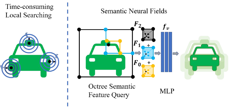
Figure 3: When querying the semantics of a vertex, intuitively, we can assign the semantics of the nearest point in the point cloud to that vertex via time-consuming local searching. The left image illustrates the concept of finding the nearest point to obtain semantics, while the right image shows our SNF method. Compared to the nearest point lookup approach, our method is much faster.

III-A3 Semantic Features Construction

To implicitly build a semantic model of scenes, our semantic information is obtained from off-the-shelf semantic segmentation or panoptic segmentation algorithms.

• Semantic Neural Fields (SNF). Following the method of geometry feature, each sampled point $x_{i}\in\mathbb{R}^{3}$ retrieve eight semantic feature vectors $F\in\mathbb{R}^{H_{2}}$, from eight corners of corresponding grids through hash table $B_{2}$ and obtain the $F_{k}$ of the point via executing tri-linear interpolation. The procedure is repeated to three last level of octree to generate $F_{2}$, $F_{1}$ and $F_{0}$. The concatenated semantic feature vector, $F_{S}=F_{2}+F_{1}+F_{0}$, are fed into MLP2 with $P$ hidden layers to predict a semantic label. Both MLP parameters and feature vectors are optimized through the self-supervised training, our supervision signal is obtained from LiDAR-based semantic segmentation algorithm RangeNet++ [29]. Relied on the feature vector interpolation and MLPs regression, the SNF is established. The SNF regression method is faster than nearest searching which is shown in Fig. 3.

• Panoptic Neural Fields (PNF). We extend above semantic paradigm to panoptic segmentation. Here, the panoptic feature vector $F$ not only implicitly contains the category label of things and stuff, but also includes instance IDs of the thing classes. The length of feature vector $F$ is $H_{2}$, we then define a ratio $\sigma$ to split the $F$, a part of the feature vector with length $\sigma H_{2}$ stores semantic label, the other part of feature vector with length $(1-\sigma)H_{2}$ represents the instance IDs of the thing. The consistent instance ID is obtained from off-the-shelf video panoptic segmentation algorithms. After we concatenate the sum-up feature vector $F_{S}$, $F_{S}$ is also split into two parts by following ratio $\sigma$. Next, we respectively feed the two uneven parts of feature vectors into two separate MLPs, to regress final panoptic labels.

III-B Training and Loss Function

As mentioned above, LiDAR is able to provide accurate range measurements. Thus, the true SDF value is directly utilized to supervise the training, we picked up the distance from sampled point to the beam endpoint as supervision signal. For semantic labels and instance labels, the output of semantic segmentation or panoptic segmentation is selected as supervision signal to form a pseudo-supervision paradigm.

We uniformly sample $N$ points along the LiDAR rays to train SDF MLP and smeantic MLPs, half of the points sampled near the objects surface and the other half sampled within the free space. For SDF value, binary cross entropy is exploited for the loss function, $L_{1}$. Given a sampled point $x_{i}\in\mathbb{R}^{3}$ and signed distance to the surface $d_{i}$, $L_{1}$ is denoted as:

$$L_{1}=\frac{log(1/(1+e^{\frac{f_{\eta}(x_{i})}{\alpha}})}{1/(1+e^{d_{i}/\alpha})}+\frac{log(1-1/(1+e^{\frac{f_{\eta}(x_{i})}{\alpha}}))}{1-1/(1+e^{d_{i}/\alpha})}$$ (2)

where $f_{\eta}(x_{i})$ represents the SDF value of geometry MLP output, $\alpha$ is a hyperparameter. Following iSDF [6], we apply Eikonal regularization to add another term, $L_{2}$, into loss function:

$$L_{2}=|\|\bigtriangledown_{x}f(x;\eta)\|-1|$$ (3)

For incremental mapping, there is a forgetting issue when the map size increases. Similar to [1], we add a regularization term, $L_{3}$, to the loss function:

$$L_{3}=\sum_{i\in N_{all}}\beta_{i}(\eta^{t}_{i}-\eta^{t-1}_{i})^{2}$$ (4)

where $N_{all}$ refers to all points in this scan. $\eta^{t}_{i}$ stands for the MLP parameter of current iteration, $\eta^{t-1}_{i}$ means the parameter of history iteration. $\beta_{i}$ is defined as a importance weight:

$$\beta_{i}=min(\beta^{t-1}_{i}+\sum\|\bigtriangledown_{\eta_{i}}L_{1}(x_{i};d_{i})\|,\beta_{m})$$ (5)

where $\beta^{t-1}_{i}$ refers to the previous importance weight, $\beta_{m}$ is a constant value to prevent gradient explosion.

For training the semantic label, given sampled point $x_{i}$ and its semantic label $s_{i}$, we leverage multi-class cross entropy as loss function :

$$L_{4}=\sum^{c-1}_{i=0}s_{i}log(S(f_{\nu}(x_{i})))$$ (6)

where $c$ is the number of semantic categories. $f_{\nu}(x_{i})$ represents the output of the semantic MLP. $S$ is Softmax function.

Then, we treat instance ID prediction as a multi-class task as well, our panoptic loss function is:

$$L_{5}=\sum^{q-1}_{i=0}y_{i}log(S(f_{\mu}(x_{i})))$$ (7)

where $q$ represents the number of instance. $y_{i}$ refers to supervision ID, which is generated from an off-the-shelf panoptic segmentation algorithm. $f_{\mu}(x_{i})$ is the output of instance MLP.

Our mapping method provides batch mode and incremental mode. The complete loss function is designed as follow based on the different mapping modes.

• Loss of incremental semantic mapping:

  $$L_{is}=L_{1}+\lambda_{2}L_{2}+\lambda_{3}L_{3}+\lambda_{4}L_{4}$$ (8)

• Loss of incremental panoptic mapping:

  $$L_{ip}=L_{1}+\lambda_{2}L_{2}+\lambda_{3}L_{3}+\lambda_{4}L_{4}+\lambda_{5}L_{5}$$ (9)

• Loss of batch-based semantic mapping:

  $$L_{bs}=L_{1}+\lambda_{2}L_{2}+\lambda_{4}L_{4}$$ (10)

• Loss of batch-based panoptic mapping:

  $$L_{bp}=L_{1}+\lambda_{2}L_{2}+\lambda_{4}L_{4}+\lambda_{5}L_{5}$$ (11)

where $\lambda_{2},\lambda_{3},\lambda_{4},\lambda_{5}$ are hyperparameters used to adjust the weight of loss function.

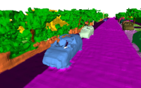
(a)

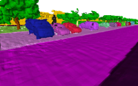
(b)

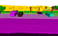
(c)

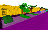
(d)

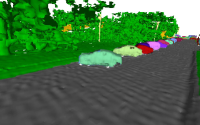
(e)

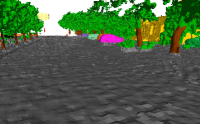
(f)

(g)

(h)

Figure 4: Our 3D reconstruction results on SemanticKITTI dataset and SemanticPOSS dataset, the first row shows the panoptic reconstruction results on the SemanticKITTI and the second row displays the panoptic reconstruction results on SemanticPOSS.

III-C Map Merge Strategy

Considering the limitations of device memory, it is often infeasible to input all the data at once to construct an entire large-scale map, especially the usage of NeRF for urban-level maps amplify this issue. Instead, our solution involves incrementally inputting data in batches to create sub-maps, which are finally fused to form a complete map. Furthermore, data collection for large-scale areas is typically obtain across multiple agents. Therefore, a fusion method is necessary to integrate submaps built on seperate agents.

We use NICP (Normal Distribution ICP) [33], which is a variant of the Iterative Closest Point (ICP) algorithm, designed for dense point cloud registration, Given point positions and the local features (normal and curvature) of the surface, alignments can be achieved.

Once different submaps have overlapping scans, we utilize NICP to compute the corresponding transformation matrix to achieve map alignment. First frame of one submap is defined as the reference frame, and the other sub-maps can be transformed into this coordinate system using the transformation matrix.

IV EXPERIMENTS

We propose an implicit semantic mapping framework which supports four working modes: incremental semantic mapping, incremental panoptic mapping, batch semantic mapping, batch panoptic mapping. We evaluate our mapping performance in batch mode in this section.

IV-A Experimental Setup

Datasets. We evaluate our method on three public outdoor LiDAR datasets. One is SemanticKITTI [34], which provide the labels of semantic segmentation and panoptic segmentation for every point cloud. The other is SemanticPOSS [35], which contains 2988 various and complicated LiDAR scans with large number of dynamic object instances. Another dataset named nuScenes [36], which has sparser LiDAR scans than other two dataset, is also examined for validating our method.

Metrics for Mapping Quality. Our evaluation metric is based on Chamfer Distance, which is a metric commonly used in computer vision community to quantify the dissimilarity between two point sets or shapes. Inspired by [37], we utilize Semantic Chamfer Distance (SCD) to evaluate the quality of our semantic mesh. We compute the distance between the points that belong to the same classes. To compute the distance for a pair of reconstructed and ground truth mesh, we randomly sample 5 million points $R$ and $T$ in our reconstructed semantic mesh and ground truth mesh, respectively. Since ground truth mesh is not provided for these two datasets, we define the labeled point cloud as ground truth. For each point $r\in R$ with the class $c_{r}$ and each point $t\in T$ with the class $c_{t}$ and , the definition of SCD is:

$$d_{t\to R}=\mathop{min}_{r\in R,c_{t}=c_{r}}\|r-t\|,d_{r\to T}=\mathop{min}_{t\in T,c_{r}=c_{t}}\|t-r\|$$ (12)

Implementation Details. For the MLPs, all the number of hidden layers of MLPs $p$ is 2. The $s_{cube}$ is 0.1 m and the $\alpha$ is 0.05, the number of sampled points for one LiDAR ray $N$ is 6. Setting $\sigma$ as $1/3$, the lengths of feature vectors $H_{1}$ and $H_{2}$ are 8 and 16, respectively. For SNF, we use feature vectors of full length to represent semantic information. For PNF, one third of $H_{2}$ is used to store semantic information and the other is used to store instance information.

IV-B Map Quality Evaluation

Qualitative Results. Fig. 4 shows our reconstruction effects on SemanticKITTI dataset and SemanticPOSS dataset. We leverage RangeNet++ to genarate semantic lablel for semantic mapping and exploit 4D-PLS algorithm to generate panoptic label for panoptic mapping. The result shows our method achieve accurate semantic mapping quality on different street scenes.

TABLE II: The F-score value of each semantic categories with different thresholds on SemanticKITTI 00.

Threshold(m)	Methods	Road	Side	Sign	Pole	Barrier	Building
0.25	Kimera(20cm) [4]	90.6	75.7	30.3	16.1	39.9	44.2
0.25	Kimera(10cm) [4]	91.2	77.7	39.8	51.9	45.0	51.1
0.25	Kimera(5cm) [4]	91.6	79.2	49.4	71.4	51.1	57.7
0.25	Lightweight [37]	89.5	74.1	53.7	58.7	53.6	50.1
0.1	LISNeRF (ours)	87.0	90.9	78.1	76.1	91.6	86.7
0.15	LISNeRF (ours)	88.5	89.7	81.4	79.0	88.1	86.5
0.20	LISNeRF (ours)	95.3	95.0	96.6	94.2	97.7	96.1

Quantitative Results. For SemanticKITTI dataset, we use the labeled point cloud as ground-truth. To the best of our knowledge, there is no existing algorithms that takes LiDAR-only input to reconstruct a semantic mesh map, we compare our approach against Kimera [4], which provides a TSDF-based semantic reconstruction and Lightweight [37], which is a semantic reconstruction method. Both methods use image sensor as input. For Kimera, we choose a voxel size of 5 cm, 10 cm, 20 cm to evaluate. By using SCD metric, we further calculate the reconstruction metric F-score [38]. TABLE II shows our quantitative reconstruction result.

TABLE III: Quantitative results of our experiments on SemanticKITTI and Semantic POSS. We show the metric on semantic map and panoptic map in the threshold 10cm, 20cm. ”Thr” = threshold ”Com” = completion, ”ACC”=accuracy, ”Ch-L1” = Champer-L1, ”Com.R” = Completion Ratio, ”SK” = SemantiKITTI, ”PO” = SemanticPOSS.

Method	Thr(m)	Datasets	Com(cm)	Acc(cm)	Ch-L1(cm)	Com.R	F-score
SHINE_Mapping [1]	0.1	SK	4.5	7.1	5.8	92.7	80.7
Ours (semantic)	0.1	SK	4.9	6.2	5.5	92.4	84.9
Ours (panoptic)	0.1	SK	5.3	6.1	5.7	91.8	85.0
SHINE_Mapping [1]	0.1	PO	7.5	7.8	7.7	80.8	74.0
Ours (semantic)	0.1	PO	8.1	6.8	7.4	79.4	77.7
Ours (panoptic)	0.1	PO	7.6	7.1	7.4	81.0	76.9
SHINE_Mapping [1]	0.2	SK	4.6	11.5	8.1	98.7	87.6
Ours(semantic)	0.2	SK	4.8	8.2	6.6	98.3	93.8
Ours(panoptic)	0.2	SK	8.1	5.3	6.7	97.6	93.6
SHINE_Mapping [1]	0.2	PO	7.5	11.8	9.7	95.3	86.7
ours (semantic)	0.2	PO	8.1	8.7	8.4	93.4	91.6
ours (panoptic)	0.2	PO	7.6	9.4	8.5	94.8	91.2

Obviously, our result achieve a better result, one of the reason is our input from LiDAR, which the precision of distance measurement is better than a RGB-D sensor. To be fair, we compare our method against SHINE_Mapping [1], which is a implicit reconstruction mapping method using LiDAR-only as input in the second experiment. We use commonly used reconstruction metric from SHINE_Mapping namely, accuracy, completion, Chamfer-L1 distance, completion ratio, F-score to evaluate our mapping quality on SemanticKITTI and SemanticPOSS. Since the two datasets don’t provide ground-truth mesh, we use point cloud as our ground-truth. As shown in TABLE III. We performed better on some metrics. Overall, we achieve slightly better results than SHINE_Mapping [1]. It’s worth noting that our map includes semantic information, whereas SHINE_Mapping does not.

(a) Submap1

(b) Submap2

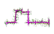
(c) Submap3

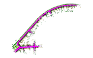
(d) Submap4

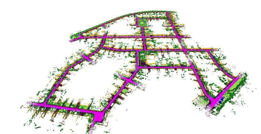
(e) The whole map

.

Figure 5: The visualization of sub-maps and the whole map

IV-C Results and Analysis of Map Merge

Our map merge experiment is conducted on SemanticKITTI sequence 00, the result is shown on Fig. 5. We divide the whole environment SemanticKITTI sequence 00 into four sections to build. From the visual result in Fig. 5, semantic submap 1 to submap 4 are successfully built, and the final entire map is successfully generated. This validates our framework based on the neural semantic fields is promising to extend to urban-level mapping scenarios. We have tested the number of overlapping parameter with 1, 5, and 10. Increasing the amount of overlapping data gradually improve the fusion results.

IV-D Evaluation for Dynamic Scenario

In highly dynamic environments, it is challenging to generate a static map without the interference of dynamic elements. As shown in Fig. 6, our method is able to eliminate certain types of the dynamic objects by introducing semantic label into the mapping paradigm.

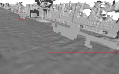
(a)

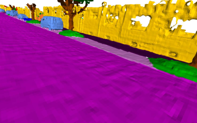
(b)

Figure 6: Illustration of the superiority of our LISNeRF for dynamic scenario. The dynamic scene is tested on SemanticKITTI, left image is generated from SHINE_Mapping, whose map is polluted by dynamic objects (shown within the red box). By enrolling semantic information, our map (right image) can eliminate ghost trails caused by dynamic objects successfully.

IV-E Generalization Ability Test

We also evaluate our method on nuScenes [36] which is collected by a 32-line LiDAR. It leads to a sparser point cloud compared to the SemanticKITTI. We test our method on scene-0061 (containing 39 frames) and scene-0916 (containing 41 frames), as shown in Fig. 7. The result shows the generalization ability of our LISNeRF framework, but it creates more holes in the map of nuScenes, this is because the sparsity of point cloud impedes the Marching Cubes to construct the space cubes.

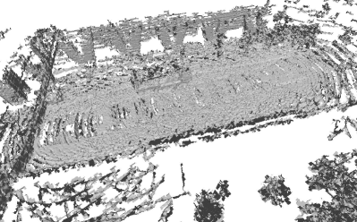
(a)

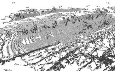
(b)

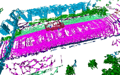
(c) scene-0061

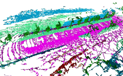
(d) scene-0796

Figure 7: Test of generalization ability on nuScenes dataset. The first row is the result of SHINE_Mapping [1], and the second row shows our reconstruction result.

V CONCLUSION

This paper proposes a novel method for large-scale implicit reconstruction with semantic information. We implicitly store geometry information and semantic information in corner of octree nodes using hash tables, then we leverage multiple MLPs to decode the feature vectors to SDF value and semantic information. We evaluate our method on three datasets and the results show that our method achieve decent mapping quality and efficiency. Besides, our framework is able to realize incremental mode and batch-based mode for semantic mapping and panoptic mapping. For large-scale mapping, we also provide a map merge method, which is helpful for multiple-agents collaborative mapping in the future tasks. We will also investigate the sparsity of input LiDAR data in the future for extending the regression ability of implicit mapping.

References

- [1] X. Zhong, Y. Pan, J. Behley, and C. Stachniss, “Shine-mapping: Large-scale 3d mapping using sparse hierarchical implicit neural representations,” in 2023 IEEE International Conference on Robotics and Automation (ICRA). IEEE, 2023, pp. 8371–8377.
- [2] R. Mascaro, L. Teixeira, and M. Chli, “Volumetric instance-level semantic mapping via multi-view 2d-to-3d label diffusion,” IEEE Robotics and Automation Letters, vol. 7, no. 2, pp. 3531–3538, 2022.
- [3] V. Cartillier, Z. Ren, N. Jain, S. Lee, I. Essa, and D. Batra, “Semantic mapnet: Building allocentric semantic maps and representations from egocentric views,” in Proceedings of the AAAI Conference on Artificial Intelligence, vol. 35, no. 2, 2021, pp. 964–972.
- [4] A. Rosinol, M. Abate, Y. Chang, and L. Carlone, “Kimera: an open-source library for real-time metric-semantic localization and mapping,” in 2020 IEEE International Conference on Robotics and Automation (ICRA). IEEE, 2020, pp. 1689–1696.
- [5] B. Mildenhall, P. P. Srinivasan, M. Tancik, J. T. Barron, R. Ramamoorthi, and R. Ng, “Nerf: Representing scenes as neural radiance fields for view synthesis,” Communications of the ACM, vol. 65, no. 1, pp. 99–106, 2021.
- [6] J. Ortiz, A. Clegg, J. Dong, E. Sucar, D. Novotny, M. Zollhoefer, and M. Mukadam, “isdf: Real-time neural signed distance fields for robot perception,” arXiv preprint arXiv:2204.02296, 2022.
- [7] Z. Zhu, S. Peng, V. Larsson, W. Xu, H. Bao, Z. Cui, M. R. Oswald, and M. Pollefeys, “Nice-slam: Neural implicit scalable encoding for slam,” in Proceedings of the IEEE/CVF Conference on Computer Vision and Pattern Recognition, 2022, pp. 12 786–12 796.
- [8] E. Sucar, S. Liu, J. Ortiz, and A. J. Davison, “imap: Implicit mapping and positioning in real-time,” in Proceedings of the IEEE/CVF International Conference on Computer Vision, 2021, pp. 6229–6238.
- [9] T. Shan and B. Englot, “Lego-loam: Lightweight and ground-optimized lidar odometry and mapping on variable terrain,” in 2018 IEEE/RSJ International Conference on Intelligent Robots and Systems (IROS). IEEE, 2018, pp. 4758–4765.
- [10] J. Lin and F. Zhang, “Loam livox: A fast, robust, high-precision lidar odometry and mapping package for lidars of small fov,” in 2020 IEEE International Conference on Robotics and Automation (ICRA). IEEE, 2020, pp. 3126–3131.
- [11] J. Behley and C. Stachniss, “Efficient surfel-based slam using 3d laser range data in urban environments.” in Robotics: Science and Systems, vol. 2018, 2018, p. 59.
- [12] W. Hess, D. Kohler, H. Rapp, and D. Andor, “Real-time loop closure in 2d lidar slam,” in 2016 IEEE international conference on robotics and automation (ICRA). IEEE, 2016, pp. 1271–1278.
- [13] I. Vizzo, X. Chen, N. Chebrolu, J. Behley, and C. Stachniss, “Poisson surface reconstruction for lidar odometry and mapping,” in 2021 IEEE International Conference on Robotics and Automation (ICRA). IEEE, 2021, pp. 5624–5630.
- [14] K. Li, Y. Tang, V. A. Prisacariu, and P. H. Torr, “Bnv-fusion: Dense 3d reconstruction using bi-level neural volume fusion,” in Proceedings of the IEEE/CVF Conference on Computer Vision and Pattern Recognition, 2022, pp. 6166–6175.
- [15] X. Chen, A. Milioto, E. Palazzolo, P. Giguere, J. Behley, and C. Stachniss, “Suma++: Efficient lidar-based semantic slam,” in 2019 IEEE/RSJ International Conference on Intelligent Robots and Systems (IROS). IEEE, 2019, pp. 4530–4537.
- [16] H. Oleynikova, Z. Taylor, M. Fehr, R. Siegwart, and J. Nieto, “Voxblox: Incremental 3d euclidean signed distance fields for on-board mav planning,” in 2017 IEEE/RSJ International Conference on Intelligent Robots and Systems (IROS). IEEE, 2017, pp. 1366–1373.
- [17] M. Grinvald, F. Furrer, T. Novkovic, J. J. Chung, C. Cadena, R. Siegwart, and J. Nieto, “Volumetric instance-aware semantic mapping and 3d object discovery,” IEEE Robotics and Automation Letters, vol. 4, no. 3, pp. 3037–3044, 2019.
- [18] T. Takikawa, J. Litalien, K. Yin, K. Kreis, C. Loop, D. Nowrouzezahrai, A. Jacobson, M. McGuire, and S. Fidler, “Neural geometric level of detail: Real-time rendering with implicit 3d shapes,” in Proceedings of the IEEE/CVF Conference on Computer Vision and Pattern Recognition, 2021, pp. 11 358–11 367.
- [19] J. Huang, S.-S. Huang, H. Song, and S.-M. Hu, “Di-fusion: Online implicit 3d reconstruction with deep priors,” in Proceedings of the IEEE/CVF Conference on Computer Vision and Pattern Recognition, 2021, pp. 8932–8941.
- [20] J. Sun, Y. Xie, L. Chen, X. Zhou, and H. Bao, “Neuralrecon: Real-time coherent 3d reconstruction from monocular video,” in Proceedings of the IEEE/CVF Conference on Computer Vision and Pattern Recognition, 2021, pp. 15 598–15 607.
- [21] S. Zhi, T. Laidlow, S. Leutenegger, and A. J. Davison, “In-place scene labelling and understanding with implicit scene representation,” in Proceedings of the IEEE/CVF International Conference on Computer Vision, 2021, pp. 15 838–15 847.
- [22] A. Kundu, K. Genova, X. Yin, A. Fathi, C. Pantofaru, L. J. Guibas, A. Tagliasacchi, F. Dellaert, and T. Funkhouser, “Panoptic neural fields: A semantic object-aware neural scene representation,” in Proceedings of the IEEE/CVF Conference on Computer Vision and Pattern Recognition, 2022, pp. 12 871–12 881.
- [23] J. Deng, X. Chen, S. Xia, Z. Sun, G. Liu, W. Yu, and L. Pei, “Nerf-loam: Neural implicit representation for large-scale incremental lidar odometry and mapping,” arXiv preprint arXiv:2303.10709, 2023.
- [24] D. Yan, X. Lyu, J. Shi, and Y. Lin, “Efficient implicit neural reconstruction using lidar,” arXiv preprint arXiv:2302.14363, 2023.
- [25] C. R. Qi, L. Yi, H. Su, and L. J. Guibas, “Pointnet++: Deep hierarchical feature learning on point sets in a metric space,” Advances in neural information processing systems, vol. 30, 2017.
- [26] H. Zhou, X. Zhu, X. Song, Y. Ma, Z. Wang, H. Li, and D. Lin, “Cylinder3d: An effective 3d framework for driving-scene lidar semantic segmentation,” arXiv preprint arXiv:2008.01550, 2020.
- [27] W. Song, Z. Liu, Y. Guo, S. Sun, G. Zu, and M. Li, “Dgpolarnet: Dynamic graph convolution network for lidar point cloud semantic segmentation on polar bev,” Remote Sensing, vol. 14, no. 15, p. 3825, 2022.
- [28] B. Wu, X. Zhou, S. Zhao, X. Yue, and K. Keutzer, “Squeezesegv2: Improved model structure and unsupervised domain adaptation for road-object segmentation from a lidar point cloud,” in 2019 international conference on robotics and automation (ICRA). IEEE, 2019, pp. 4376–4382.
- [29] A. Milioto, I. Vizzo, J. Behley, and C. Stachniss, “Rangenet++: Fast and accurate lidar semantic segmentation,” in 2019 IEEE/RSJ international conference on intelligent robots and systems (IROS). IEEE, 2019, pp. 4213–4220.
- [30] R. Marcuzzi, L. Nunes, L. Wiesmann, J. Behley, and C. Stachniss, “Mask-based panoptic lidar segmentation for autonomous driving,” IEEE Robotics and Automation Letters, vol. 8, no. 2, pp. 1141–1148, 2023.
- [31] J. Li, X. He, Y. Wen, Y. Gao, X. Cheng, and D. Zhang, “Panoptic-phnet: Towards real-time and high-precision lidar panoptic segmentation via clustering pseudo heatmap,” in Proceedings of the IEEE/CVF Conference on Computer Vision and Pattern Recognition, 2022, pp. 11 809–11 818.
- [32] M. Aygun, A. Osep, M. Weber, M. Maximov, C. Stachniss, J. Behley, and L. Leal-Taixé, “4d panoptic lidar segmentation,” in Proceedings of the IEEE/CVF Conference on Computer Vision and Pattern Recognition, 2021, pp. 5527–5537.
- [33] J. Serafin and G. Grisetti, “Nicp: Dense normal based point cloud registration,” in 2015 IEEE/RSJ International Conference on Intelligent Robots and Systems (IROS). IEEE, 2015, pp. 742–749.
- [34] J. Behley, M. Garbade, A. Milioto, J. Quenzel, S. Behnke, C. Stachniss, and J. Gall, “SemanticKITTI: A Dataset for Semantic Scene Understanding of LiDAR Sequences,” in Proc. of the IEEE/CVF International Conf. on Computer Vision (ICCV), 2019.
- [35] Y. Pan, B. Gao, J. Mei, S. Geng, C. Li, and H. Zhao, “Semanticposs: A point cloud dataset with large quantity of dynamic instances,” in 2020 IEEE Intelligent Vehicles Symposium (IV). IEEE, 2020, pp. 687–693.
- [36] H. Caesar, V. Bankiti, A. H. Lang, S. Vora, V. E. Liong, Q. Xu, A. Krishnan, Y. Pan, G. Baldan, and O. Beijbom, “nuscenes: A multimodal dataset for autonomous driving,” arXiv preprint arXiv:1903.11027, 2019.
- [37] M. Herb, T. Weiherer, N. Navab, and F. Tombari, “Lightweight semantic mesh mapping for autonomous vehicles,” in 2021 IEEE International Conference on Robotics and Automation (ICRA). IEEE, 2021, pp. 6732–3738.
- [38] A. Knapitsch, J. Park, Q.-Y. Zhou, and V. Koltun, “Tanks and temples: Benchmarking large-scale scene reconstruction,” ACM Transactions on Graphics (ToG), vol. 36, no. 4, pp. 1–13, 2017.