Coalescence sum rule and the electric charge- and strangeness-dependences of directed flow in heavy ion collisions

Abstract

The rapidity-odd directed flows ($v_{\rm 1}$) of identified hadrons are expected to follow the coalescence sum rule when the created matter is initially in parton degrees of freedom and then hadronizes through quark coalescence. A recent study has considered the $v_{\rm 1}$ of produced hadrons that do not contain $u$ or $d$ constituent quarks. It has constructed multiple hadron sets with a small mass difference but given difference in electric charge $\Delta q$ and strangeness $\Delta S$ between the two sides, where a nonzero and increasing $\Delta v_{\rm 1}$ with $\Delta q$ has been proposed to be a consequence of electromagnetic fields. In this study, we examine the consequence of coalescence sum rule on the $\Delta v_{\rm 1}$ of the hadron sets in the absence of electromagnetic fields. We find that in general $\Delta v_{\rm 1}\neq 0$ for a hadron set with nonzero $\Delta q$ and/or $\Delta S$ due to potential $v_{\rm 1}$ differences between $\bar{u}$ and $\bar{d}$ and between $s$ and $\bar{s}$ quarks. We further propose methods to extract the coefficients for the $\Delta q$- and $\Delta S$-dependences of the direct flow difference, where a nonzero constant term would indicate the breaking of the coalescence sum rule. The extraction methods are then demonstrated with transport model results.

I Introduction

The properties of the quark-gluon plasma produced in relativistic heavy ion collisions can be studied with the directed flow ($v_{\rm 1}$) Li and Ko (1998); Stöcker (2005); Nara et al. (2016); Luo et al. (2020). For example, $v_{\rm 1}$ is found to be a sensitive probe of the equation of state of the produced matter Sorge (1997); Herrmann et al. (1999), and $v_{\rm 1}$ of heavy flavors Das et al. (2017) is expected to be sensitive to the strong electromagnetic field in the early stage of noncentral heavy ion collisions.

The coalescence sum rule is often found to describe well the relations of anisotropic flows of different hadron species in heavy ion collisions at high energies Molnár and Voloshin (2003); Adams and et. al (2004); Abelev and et. al. (2007); Adler and et. al. (2003); Adare and et. al. (2007); Abelev and et. al. (2015). For collisions where the dynamics of anisotropic flows is dominated by parton interactions, quark coalescence relates the hadron flow directly to the flows of the hadron’s constituent quarks Lin and Ko (2002); Molnár and Voloshin (2003); Lin and Molnár (2003). When the constituent quarks in a hadron are comoving with each other and the quark coalescence probability is small, the hadron elliptic flow $v_{2}$ follows the coalescence sum rule at leading order Molnár and Voloshin (2003); Lin and Molnár (2003); Lin (2011). The same formulation can be extended to the directed flow. When we neglect the mass difference of the constituent quarks Lin and Molnár (2003), the coalescence sum rule is simply given by Molnár and Voloshin (2003)

$$v_{n}^{H}(p_{\rm T}^{H})=\sum_{j}v_{n,j}(p_{\rm T}),{\rm~{}with~{}}p_{\rm T}^{H}=N_{cq}\,p_{\rm T}.$$ (1)

In the above, $n=1$ for $v_{\rm 1}$ and $n=2$ for $v_{2}$, $v_{n,j}(p_{\rm T})$ represents the flow $v_{n}$ of constituent quark $j$ at the quark transverse momentum $p_{\rm T}$, while $N_{cq}$ is the number of constituent quarks (NCQ) of the hadron species $H$. Furthermore, if the quark $v_{n}(p_{\rm T})$ is the same for each constituent quark of hadron species $H$, Eq.(1) reduces to the most used form of the NCQ scaling: $v_{n}^{H}(N_{cq}\,p_{\rm T})=N_{cq}\,v_{n}(p_{\rm T})$.

It has been proposed Adamczyk and et. al. (2018) that the direct flows of hadrons whose constituent quarks are all produced quarks can be properly combined to better test the coalescence sum rule. In contrast to produced quarks, hadrons containing $u$ and/or $d$ quarks get contributions from slowed-down (or transported) $u$ and $d$ quarks in the incoming nuclei Dunlop et al. (2011); Nayak et al. (2019), which complicate the flow analysis. Our study here has been motivated by a recent study Sheikh et al. (2022), which further considered the $v_{\rm 1}$ difference of various combinations of hadron sets consisting of seven produced hadron species: $K^{-},\phi,\bar{p},\bar{\Lambda},{\bar{\Xi}}^{+},\Omega^{-}$, and ${\bar{\Omega}}^{+}$. For example, one of the combinations is $v_{\rm 1}[{\bar{\Lambda}}]-(v_{\rm 1}[\phi]/2+2v_{\rm 1}[\bar{p}]/3)$. That study focused on the dependence of the $v_{\rm 1}$ difference on the electric charge difference $\Delta q$ and the strangeness difference $\Delta S$ of the hadron set combinations. A nonzero $v_{\rm 1}$ difference at nonzero $\Delta q$ was considered as the breaking of the coalescence sum rule and proposed to be a consequence of the electromagnetic fields Sheikh et al. (2022); STAR (2023), especially if the $v_{\rm 1}$ difference increases with $\Delta q$. The study also recognized the need for further investigation if a systematic dependence of the $v_{\rm 1}$ difference on $\Delta S$ is observed Sheikh et al. (2022).

In this study, we examine in detail the $v_{\rm 1}$ difference of various combinations of these seven hadron species. Note that the $v_{1}$ throughout this study refers to the rapidity-odd directed flow, although $v_{\rm 1}$ contains both rapidity-odd and rapidity-even components where the rapidity-even directed flow originates from event-by-event fluctuations. In addition, since we only consider light quarks, which constituent masses are not too different, we neglect the effect of different quark masses on the coalescence sum rule Lin and Molnár (2003) and thus start the analysis from Eq.(1). The paper is organized as follows. In Sec. II, we derive the coalescence sum rule relationships between the $v_{\rm 1}$ difference of each hadron set and the quark $v_{\rm 1}$. In Sec. III, we present two methods to extract the dependences of the $v_{\rm 1}$ difference on the electric charge difference $\Delta q$ and the strangeness difference $\Delta S$, and in Sec. IV we demonstrate the extraction methods with the numerical $v_{\rm 1}$ results from a multi-phase transport (AMPT) model. Finally, we summarize in Sec. V.

II Coalescence sum rule relations for the $v_{\rm 1}$ difference of a hadron set

Set #	$\Delta q_{ud}$	$\Delta S$	$\Delta q$	L (left side)	R (right side)
1	0	0	0	$v_{\rm 1}[K^{-}(\bar{u}s)]+v_{\rm 1}[\overline{\Lambda}(\bar{u}\bar{d}\bar{s})]$	$v_{\rm 1}[\bar{p}(\bar{u}\bar{u}\bar{d})]+v_{\rm 1}[\phi(s\bar{s})]$
2	0	0	0	$v_{\rm 1}\big{[}\overline{\Lambda}(\bar{u}\bar{d}\bar{s})\big{]}$	$\frac{1}{2}v_{\rm 1}[\bar{p}(\bar{u}\bar{u}\bar{d})]+\frac{1}{2}v_{\rm 1}[\overline{\Xi}^{+}(\overline{d}\bar{s}\bar{s})]$
3	0	0	0	$\frac{1}{3}v_{\rm 1}[\Omega^{-}(sss)]+\frac{1}{3}v_{\rm 1}[\overline{\Omega}^{+}(\bar{s}\bar{s}\bar{s})]$	$v_{\rm 1}[\phi(s\bar{s})]$
4	0	1	1/3	$\frac{1}{2}v_{\rm 1}[\phi(s\bar{s})]$	$\frac{1}{3}v_{\rm 1}[\Omega^{-}(sss)]$
5A	1/3	1	2/3	$\frac{1}{2}v_{\rm 1}[\phi(s\bar{s})]+\frac{1}{3}v_{\rm 1}[\bar{p}(\bar{u}\bar{u}\bar{d})]$	$v_{\rm 1}\big{[}K^{-}(\bar{u}s)\big{]}$
5B	1/3	1	2/3	$v_{\rm 1}\big{[}\overline{\Lambda}(\bar{u}\bar{d}\bar{s})\big{]}$	$\frac{1}{2}v_{\rm 1}[\phi(s\bar{s})]+\frac{2}{3}v_{\rm 1}[\bar{p}(\bar{u}\bar{u}\bar{d})]$

Table 1: List of several hadron sets, where the left side and right side have the same total number of $\bar{u}$ and $\bar{d}$ quarks and the same total number of $s$ and $\bar{s}$ quarks (after including the weights). $\Delta q$, $\Delta q_{ud}$ and $\Delta S$ represent the difference in the electric charge, electric charge from $\bar{u}$ and $\bar{d}$ quarks, and strangeness number, respectively, between the two sides. Note that sets 1 to 4 and set 5A are independent of each other, while set 5B is not independent of them.

In this study, we only consider produced hadrons whose constituent quarks consist of $\bar{u}$, $\bar{d}$, $s$ and $\bar{s}$ quarks. Table 1 lists several such hadron sets, where for each combination the left side and the right side have the same total number of $\bar{u}$ and $\bar{d}$ quarks and the same total number of $s$ and $\bar{s}$ quarks (after including the weighting factors). For a given hadron set, let $N_{i}^{L}$ and $N_{i}^{R}$ be the total number of constituent quarks of flavor $i$ in each hadron multiplied by the weighting factor of the hadron on the left side and right side, respectively. We then write

$$\Delta N_{i}\equiv N_{i}^{L}-N_{i}^{R}$$ (2)

as the difference of $N_{i}$ between the two sides. Then each hadron set in Table 1 satisfies the following relations:

$$\Delta N_{\bar{u}}+\Delta N_{\bar{d}}=0,~{}\Delta N_{s}+\Delta N_{\bar{s}}=0.$$ (3)

For example, set 5A has $N_{\bar{u}}^{L}=2/3$, $N_{\bar{d}}^{L}=1/3$, $N_{s}^{L}=N_{\bar{s}}^{L}=1/2$, $N_{\bar{u}}^{R}=1$, and $N_{s}^{R}=1$. Similar to Eq.(2), we can define the differences of the total electric charge in $\bar{u}$ and $\bar{d}$ quarks ($q_{ud}$), the total strangeness $S$, and the total electric charge $q$, between the two sides as

$$\Delta q_{ud} \equiv q_{ud}^{L}-q_{ud}^{R}=\Delta N_{\bar{d}},$$

$$\Delta S \equiv S^{L}-S^{R}=2\Delta N_{\bar{s}},$$

$$\Delta q \equiv q^{L}-q^{R}=\Delta q_{ud}+\frac{1}{3}\Delta S,$$ (4)

respectively. The values of $\Delta q_{ud}$, $\Delta S$, and $\Delta q$ for each hadron set are given in Table 1, where the left side and right side are shown with the constituent quark content and the weighting factor of each hadron. Because of Eq.(3), the mass difference (after including the weighting factors) between the two sides is small for most of these hadron sets. Note that sets 1, 2, and 3 each have identical constituent quark content on the left and right sides and thus satisfy $\Delta q_{ud}=\Delta q=\Delta S=0$. On the other hand, sets 4, 5A and 5B each have a nonzero charge difference and/or a nonzero strangeness difference between the two sides. One can show that the conditions of Eq.(3) lead to the following general hadron set:

$$a_{1}\,K^{-}+a_{2}\,\phi+a_{3}\,\bar{p}+a_{4}\,\bar{\Lambda}-(a_{1}+3a_{3}+2a_{4})\,{\bar{\Xi}}^{+}$$

$$+a_{5}\,\Omega^{-}+\left(\frac{a_{1}}{3}-\frac{2a_{2}}{3}+2a_{3}+a_{4}-a_{5}\right){\bar{\Omega}}^{+}=0,$$ (5)

where $a_{i}$ are arbitrary constants; as a result, there are only five sets of independent hadron sets Sheikh et al. (2022). Sets 1 to 4 and 5A in Table 1 give one example of the five independent sets; so do sets 1 to 4 and 5B. However, sets 1, 5A, and 5B are not independent of each other, since the $v_{\rm 1}$ difference between the two sides of set 5B can be written as that of set 5A plus that of set 1. With sets 1 to 4 and 5A (or 5B) in Table 1, one can construst all the hadron sets of earlier studies Sheikh et al. (2022); STAR (2023).

We now apply the coalescence sum rule in Eq.(1) to evaluate the difference between the $v_{\rm 1}$ from two sides of a given hadron set. Since we neglect the mass difference of $u/d/s$ constituent quarks, the quarks coalescing to form a hadron have the same $p_{\rm T}$. If we only consider quarks at a given $p_{\rm T}$, then they will form mesons at $p_{\rm T}^{M}=2p_{\rm T}$ and (anti)baryons at $p_{\rm T}^{B}=3p_{\rm T}$; this is why we have chosen the $p_{\rm T}$ range as $[0,2]$ GeV$/c$ for mesons and $[0,3]$ GeV$/c$ for (anti)baryons for the analysis of the model calculations in Sec. IV. The difference between the $v_{\rm 1}$ from two sides of a given hadron set is then given by

$$\Delta v_{\rm 1}\equiv v_{\rm 1}^{L}-v_{\rm 1}^{R}=\sum_{i}\Delta N_{i}\;v_{\rm 1,i}\;,$$ (6)

where $v_{\rm 1,i}$ represents the $v_{1}$ of quark flavor $i$ with $i\in\{\bar{u},\bar{d},s,\bar{s}\}$ and we have skipped the $p_{\rm T}$ argument in the $v_{1}(p_{\rm T})$ notations for brevity. Note that although the above relation is written for a given quark $p_{\rm T}$, it still applies when quarks are selected within a given $p_{\rm T}$ range, in which case $v_{\rm 1,i}$ just represents the average $v_{1}$ of quark flavor $i$ within that $p_{\rm T}$ range. With Eqs.(3)-(4), we further obtain

$$\Delta v_{\rm 1}=(v_{1,\bar{d}}-v_{1,\bar{u}})\Delta q_{ud}+\left(\frac{v_{1,\bar{s}}-v_{1,s}}{2}\right)\Delta S$$

$$=(v_{1,\bar{d}}\!-\!v_{1,\bar{u}})\Delta q\!+\!\left(\frac{v_{1,\bar{s}}\!-\!v_{1,s}}{2}\!-\!\frac{v_{1,\bar{d}}\!-\!v_{1,\bar{u}}}{3}\right)\Delta S.$$ (7)

$v_{\rm 1}$ observables such as those appearing in Eqs.(6)-(7) are functions of the hadron rapidity $y$. The rapidity-odd $v_{\rm 1}$ around mid-rapidity is often fit with a linear function in rapidity, with the only parameter being the slope ($v_{\rm 1}^{\prime}$). If we assume that the rapidity of a hadron formed by quark coalescence is the same as that of the coalescing quarks (which have the same rapidity due to the comoving requirement), we can then take the derivative with respect to $y$ and obtain

$$\Delta v_{\rm 1}^{\prime}=\sum_{i}\Delta N_{i}\;v^{\prime}_{\rm 1,i}\;,{\rm~{}with~{}}v_{\rm 1}^{\prime}\equiv\frac{dv_{\rm 1}}{dy}{\Big{|}}_{y=0}.$$ (8)

The above just relates the difference of the $v_{\rm 1}$ slope parameters from two sides of a hadron set to the quark $v_{\rm 1}$ slope parameters. We also have

$$\Delta v_{\rm 1}^{\prime}=(v^{\prime}_{1,\bar{d}}-v^{\prime}_{1,\bar{u}})\Delta q_{ud}+\left(\frac{v^{\prime}_{1,\bar{s}}-v^{\prime}_{1,s}}{2}\right)\Delta S$$

$$=(v^{\prime}_{1,\bar{d}}\!-\!v^{\prime}_{1,\bar{u}})\Delta q\!+\!\left(\frac{v^{\prime}_{1,\bar{s}}\!-\!v^{\prime}_{1,s}}{2}\!-\!\frac{v^{\prime}_{1,\bar{d}}\!-\!v^{\prime}_{1,\bar{u}}}{3}\right)\Delta S.$$ (9)

Therefore, the difference of the $v_{\rm 1}$ slope parameters of a hadron set depends linearly on both $\Delta q_{ud}$ and $\Delta S$, where the corresponding coefficient is given by the difference of the quark-level $v_{\rm 1}$ slope parameters. It is also clear that the interpretation of the coefficients is simpler if we use $\Delta q_{ud}$ instead of $\Delta q$ for the electric charge difference. When one assumes that $\bar{u}$ and $\bar{d}$ quarks have the same $v_{\rm 1}$ slope and that $s$ and $\bar{s}$ have the same $v_{\rm 1}$ slope Sheikh et al. (2022), all the coefficients in Eq.(9) would be zero. However, $\Delta v_{\rm 1}^{\prime}\neq 0$ in general according to the coalescence sum rule when $\Delta q$ and/or $\Delta S$ is nonzero, which is the case for sets 4, 5A, and 5B in Table 1.

III Extracting coefficients for the $\Delta q$ and $\Delta S$ dependences

Since there are five independent sets, e.g., sets 1 to 4 and 5A, one will get five independent $\Delta v_{\rm 1}^{\prime}$ data points from the experimental measurement (for a given event class of a given collision system). One can then extract the $\Delta q$ and $\Delta S$ coefficients, which reflect the quark-level $v_{\rm 1}$ slope differences. One way to extract the coefficients is to simply fit the five data points; this is the 5-set method. Alternatively, since sets 1 to 3 all have $\Delta q_{ud}=\Delta q=\Delta S=0$, we can combine these three data points into one and then fit three data points (the combined point plus sets 4 and 5); this is the 3-set method.

For certain collision systems, the coalescence sum rule may not be satisfied, e.g., if $v_{\rm 1}$ is not dominated by parton dynamics or the flows are affected by other effects such as the electromagnetic field. Since Eq.(9) based on the coalescence sum rule gives $\Delta v_{\rm 1}^{\prime}=0$ for $\Delta q_{ud}=\Delta S=0$ (and for $\Delta q=\Delta S=0$), we use the following modified equations to fit the 5-set or 3-set $\Delta v_{\rm 1}^{\prime}$ values:

$$\Delta v_{\rm 1}^{\prime} = c_{0}+c_{q}\Delta q_{ud}+c_{S}\Delta S$$ (10)

$$= c_{0}^{\star}+c_{q}^{\star}\Delta q+c_{S}^{\star}\Delta S.$$ (11)

This way, a nonzero value of the new intercept term $c_{0}$ or $c_{0}^{\star}$ would mean the breaking of coalescence sum rule. According to Eq.(9), the coalescence sum rule predicts the following:

$$c_{0}=c_{0}^{\star}=0,$$

$$c_{q}=c_{q}^{\star}=v^{\prime}_{1,\bar{d}}-v^{\prime}_{1,\bar{u}}\;,$$

$$c_{S}=\frac{v^{\prime}_{1,\bar{s}}-v^{\prime}_{1,s}}{2},~{}~{}c_{S}^{\star}=c_{S}-\frac{c_{q}}{3}.$$ (12)

In the 3-set method, we combine the three $\Delta v_{\rm 1}^{\prime}$ points (from sets 1 to 3) into one point. Because these three data sets can have very different statistical errors ($e_{i}$) or hadron counts, we average the central values of the three $\Delta v_{\rm 1}^{\prime}$ data points by using $1/e_{i}^{2}$ as the weight, and we calculate the statistical error of the combined data point as $1/\sqrt{1/e_{1}^{2}+1/e_{2}^{2}+1/e_{3}^{2}}$. Let us denote the combined data point as $\Delta v_{\rm 1,1-3}^{\prime}$; we also denote the data point from sets 4 and 5 (5A or 5B) as $\Delta v_{\rm 1,4}^{\prime}$ and $\Delta v_{\rm 1,5}^{\prime}$, respectively. Eq.(10) then leads to $\Delta v_{\rm 1,1-3}^{\prime}=c_{0},\Delta v_{\rm 1,4}^{\prime}=c_{0}+c_{S},\Delta v_{\rm 1,5}^{\prime}=c_{0}+c_{q}/3+c_{S}$. Therefore, the coefficients in Eq.(10) for the 3-set method are given by

$$c_{0} = \Delta v_{\rm 1,1-3}^{\prime}\;,~{}~{}c_{q}=-3(\Delta v_{\rm 1,4}^{\prime}-\Delta v_{\rm 1,5}^{\prime}),$$

$$c_{S} = -\Delta v_{\rm 1,1-3}^{\prime}+\Delta v_{\rm 1,4}^{\prime}.$$ (13)

Similarly, the coefficients in Eq.(11) for the 3-set method are given by

$$c_{0}^{\star} = \Delta v_{\rm 1,1-3}^{\prime}\;,~{}~{}c_{q}^{\star}=-3(\Delta v_{\rm 1,4}^{\prime}-\Delta v_{\rm 1,5}^{\prime}),$$

$$c_{S}^{\star} = -\Delta v_{\rm 1,1-3}^{\prime}+2\Delta v_{\rm 1,4}^{\prime}-\Delta v_{\rm 1,5}^{\prime}.$$ (14)

IV Tests with a transport model

We now use the AMPT model Lin et al. (2005) as an example to demonstrate the $v_{\rm 1}$ analysis and extraction of the $\Delta q$ and $\Delta S$ coefficients. We use the default version of the AMPT model to simulate mid-central (10-50$\%$) Au+Au collisions at $\sqrt{s_{\rm NN}}$ = 7.7, 14.5, 27, 54.4, and 200 GeV. The event centrality is determined from the multiplicity of charged hadrons within the pseudorapidity range $|\eta|<1/2$. For simplicity, we calculate $v_{\rm 1}$ with respect to the reaction plane angle ($\Psi_{RP}$) as $v_{\rm 1}=\langle{\rm cos}(\phi-\Psi_{RP})\rangle$, where $\phi$ is the azimuthal angle of a hadron’s momentum Voloshin and Zhang (1996); Poskanzer and Voloshin (1998).

As an example, Fig. 1 shows the rapidity dependence of $v_{\rm 1}$ for hadron set 2, where $v_{\rm 1}^{L}=v_{\rm 1}[\bar{\Lambda}]$ and $v_{\rm 1}^{R}=v_{\rm 1}[{\bar{p}}]/2+v_{\rm 1}[{\bar{\Xi}}^{+}]/2$. We then fit their difference $\Delta v_{\rm 1}$ (circles) within $|y|<1.5$ at each energy with a rapidity-odd linear function of $y$ to obtain the slope difference $\Delta v_{\rm 1}^{\prime}$. Note that for hadron set 2 with $\Delta q_{ud}=\Delta q=\Delta S=0$, we expect $\Delta v_{\rm 1}^{\prime}=0$ from Eq.(9). However, this is not the case for the default-AMPT model results at low energies in Fig. 1.

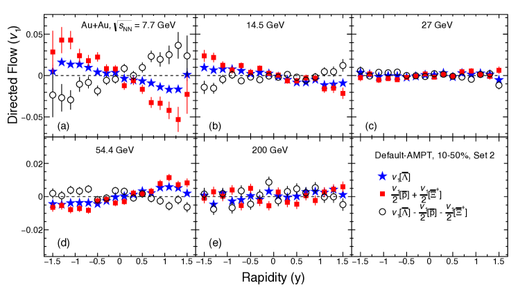
Figure 1: Directed flows of hadron set 2 in Table 1: $v_{\rm 1}[\bar{\Lambda}]$, $v_{\rm 1}[{\bar{p}}]/2+v_{\rm 1}[{\bar{\Xi}}^{+}]/2$, and their difference as functions of rapidity from the default AMPT model for 10-50% central Au+Au collisions at $\sqrt{s_{\rm NN}}$ = 7.7, 14.5, 27, 54.4 and 200 GeV.

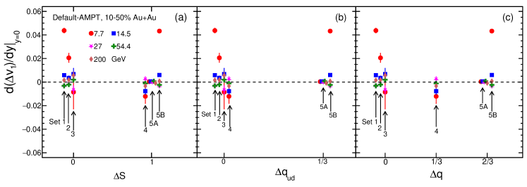
Figure 2: The difference of the $v_{\rm 1}$ slopes at mid-rapidity for each hadron set in Table 1 versus (a) $\Delta S$, (b) $\Delta q_{ud}$, and (c) $\Delta q$ from the default AMPT model for 10-50$\%$ central Au+Au collisions at several energies. Data points at the same horizontal value are often slightly shifted horizontally for better visibility.

Figure 2 shows the slope difference $\Delta v_{\rm 1}^{\prime}$ of each set at the five energies as functions of (a) $\Delta S$, (b) $\Delta q_{ud}$, and (c) $\Delta q$. Since $\Delta v_{\rm 1}^{\prime}$ depends linearly on both $\Delta q$ and $\Delta S$, one cannot determine the coefficient $c_{q}$ (or $c_{S}$) by simply performing a one-dimensional linear fit of the $\Delta q$ plot such as Fig. 2(b) (or the $\Delta S$ plot such as Fig. 2(a)) STAR (2023). Note that a one-dimensional linear fit as a function of $\Delta q$ performed at the same $\Delta S$ value Sheikh et al. (2022) would be better. Here, we propose to extract the $c_{q}$ and $c_{S}$ coefficients by describing the $\Delta v_{\rm 1}^{\prime}$ data with a two-dimensional plane (over the $\Delta q$-$\Delta S$ space). We can use the 5-set method by fitting five independent data points with the relation of Eq.(10). As a demonstration, Fig. 3(a) shows the fitting of five data points (from sets 1 to 4 and set 5A) from the AMPT model at $\sqrt{s_{\rm NN}}$ =14.5 GeV with the 5-set method. Alternatively, we can use the 3-set method, where we fit the combined data point for sets 1 to 3 and the data points from set 4 and set 5A (or 5B). This is demonstrated in Fig. 3(b), where the data point at $\Delta q_{ud}=\Delta S=0$ represents an average of the three corresponding data points shown in Fig. 3(a) (from the three hadrons sets with identical constituent quark content on the two sides). The resultant coefficients obtained from the 5-set method and the 3-set method are practically the same, as we can see from the almost identical planes in Figs. 3(a) and (b). On the other hand, the 3-set method has an advantage in that the coefficients can be determined by Eq.(13) or Eq.(14) without the need to perform a fit.

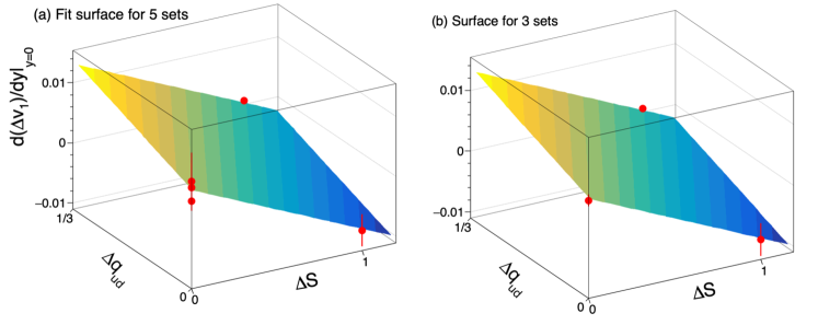
Figure 3: The fit plane to extract the $\Delta v_{\rm 1}^{\prime}$ dependences on $\Delta q_{ud}$ and $\Delta S$ as shown in Eq.(10) using (a) the 5-set method and (b) the 3-set method. The data points, corresponding to sets 1 to 4 and set 5A in Table 1, come from the default AMPT model for mid-central (10-50$\%$) Au+Au collisions at $\sqrt{s_{\rm NN}}$ = 14.5 GeV.

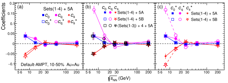
Figure 4: Comparisons of the coefficients extracted from AMPT results with the 5-set method as functions of colliding energy: (a) $c_{0},c_{q},c_{S}$ compared with $c_{0}^{\star},c_{q}^{\star},c_{S}^{\star}$ from sets 1 to 4 and 5A, (b) $c_{0},c_{q},c_{S}$ values, and (c) $c_{0}^{\star},c_{q}^{\star},c_{S}^{\star}$ values from sets 1 to 4 and 5A compared with those from sets 1 to 4 and 5B. Panel (b) also shows the coefficients from the 3-set method (black symbols).

In Fig. 4, we compare the coefficients extracted from the AMPT model results for semi-central Au+Au collisions versus the colliding energy. Figure 4(a) compares $c_{0},c_{q},c_{S}$ in Eq.(10) (filled symbols) with $c_{0}^{\star},c_{q}^{\star},c_{S}^{\star}$ in Eq.(11) (open symbols) extracted with the 5-set method using sets 1 to 4 and 5A. We confirm the relations of Eqs.(13)-(14) in that fitting the data versus $\Delta q_{ud}$ or $\Delta q$ does not affect the $c_{0}$ and $c_{q}$ coefficients but gives different $c_{S}$ values. We also see that the coefficients here exhibit a clear energy dependence, especially at low energies. In particular, at 7.7GeV the nonzero intercept $c_{0}$ indicates the breaking of the coalescence sum rule; as a result, one cannot trust Eq.(12) and interpret the $c_{q}$ and $c_{S}$ coefficients as quark-level $v_{\rm 1}^{\prime}$ differences there.

Although there are only five independent hadron sets for this study, they can be written in different combinations Sheikh et al. (2022); STAR (2023). For example, one can choose them as sets 1 to 4 and set 5B (instead of 5A). The corresponding coefficients are shown in Fig. 4(b) for $c_{0},c_{q},c_{S}$ and in Fig. 4(c) for $c_{0}^{\star},c_{q}^{\star},c_{S}^{\star}$, in comparison with those extracted from sets 1 to 4 and set 5A. We see in Fig. 4(b) that the $c_{q}$ value depends on the choice of the five sets, while $c_{0}$ and $c_{S}$ values do not. This is expected from Eq.(13), which shows that set 5 only affects the $c_{q}$ value. We also show in Fig. 4(b) the coefficients extracted with the 3-set method of Eq.(13) for hadron sets 1 to 4 and set 5A; they are essentially the same as those extracted with the 5-set method. Note that, since hadron set 5B in Table 1 is a combination of set 1 and set 5A, the difference in the $c_{q}$ value from using set 5B and that from using set 5A is given by (three times) the $\Delta v_{\rm 1}^{\prime}$ value of set 1, which is shown in Fig. 2 to be nonzero at low energies. In Fig. 4(c), we see that both the $c_{q}^{\star}$ and $c_{S}^{\star}$ values depend on the choice of using set 5A or 5B. This is consistent with the expectations of Eq.(14), and the nonzero differences are again due to the nonzero $\Delta v_{\rm 1}^{\prime}$ of set 1 (which would be zero if the coalescence sum rule were exact). Therefore, getting different coefficient values from different choices of five independent hadron sets, like a nonzero $c_{0}$ value, indicates the breaking of the coalescence sum rule.

V Conclusions

In this study, we start from the coalescence sum rule and derive the relations between the rapidity-odd directed flows ($v_{\rm 1}$) of different hadron sets. Following earlier studies, we consider seven species of produced hadrons (those without $u$ or $d$ constituent quarks): $K^{-},\phi,\bar{p},\bar{\Lambda},{\bar{\Xi}}^{+},\Omega^{-}$, and ${\bar{\Omega}}^{+}$, where the two sides of each hadron set have the same total number of $\bar{u}$ and $\bar{d}$ quarks and the same total number of $s$ and $\bar{s}$ quarks after including the weighting factors. Earlier studies have proposed that a nonzero directed flow difference ($\Delta v_{\rm 1}$) between the two sides of the hadron sets, especially a dependence on the electric charge difference $\Delta q$, means the breaking of the coalescence sum rule and would indicate the effect of the electromagnetic fields. Here we show that the coalescence sum rule only leads to zero $\Delta v_{\rm 1}$ for a hadron set if its two sides have identical constituent quark content (or equivalently if $\Delta q=\Delta S=0$). In general, $\Delta v_{\rm 1}$ depends linearly on both $\Delta S$ and $\Delta q$, or on both $\Delta S$ and $\Delta q_{ud}$ (the electric charge difference in $\bar{u}$ and $\bar{d}$ constituent quarks). The same is true for $\Delta v_{\rm 1}^{\prime}$, the difference of the $v_{\rm 1}$ slopes around mid-rapidity ($v_{\rm 1}^{\prime}$). For $\Delta v_{\rm 1}^{\prime}$, the coefficient $c_{q}$ for its $\Delta q_{ud}$ dependence reflects the $\bar{d}$ and $\bar{u}$ quark $v_{\rm 1}^{\prime}$ difference, while the coefficient $c_{S}$ for its $\Delta S$ dependence reflects half the $\bar{s}$ and $s$ quark $v_{\rm 1}^{\prime}$ difference.

Since there are only five independent such hadron sets, there will be five independent $\Delta v_{\rm 1}^{\prime}$ data points from the measurement of a given collision system. We propose to fit the data points with a two-dimensional plane in the functional form of $c_{0}+c_{q}\Delta q_{ud}+c_{S}\Delta S$ to extract the three coefficients, where a nonzero intercept $c_{0}$ indicates the breaking of the coalescence sum rule. In the 5-set method, one simply fits the five data points with this function. In the more elegant 3-set method, we combine the data points from the three sets at $\Delta q_{ud}=\Delta S=0$ into one and then obtain the coefficients analytically. We have also used results from the default version of the AMPT model for mid-central Au+Au collisions at various energies to demonstrate the extraction methods. The 5-set method and the 3-set method are shown to extract essentially the same coefficients. In addition, we show that the extracted coefficients may depend on the choice of the five independent hadron sets, and getting different coefficients from different choices indicates the breaking of the coalescence sum rule. This work provides the baseline relations for the $v_{\rm 1}$ difference of various hadron sets from the coalescence sum rule. Further work is needed to consider the possible effect of the electromagnetic fields.

References

- Li and Ko (1998) B.-A. Li and C. M. Ko, Phys. Rev. C 58, R1382 (1998), URL https://link.aps.org/doi/10.1103/PhysRevC.58.R1382.
- Stöcker (2005) H. Stöcker, Nuclear Physics A 750, 121 (2005), URL https://doi.org/10.1016%2Fj.nuclphysa.2004.12.074.
- Nara et al. (2016) Y. Nara, H. Niemi, A. Ohnishi, and H. Stöcker, Phys. Rev. C 94, 034906 (2016), URL https://link.aps.org/doi/10.1103/PhysRevC.94.034906.
- Luo et al. (2020) X. Luo, S. Shi, N. Xu, and Y. Zhang, Particles 3, 278 (2020).
- Sorge (1997) H. Sorge, Phys. Rev. Lett. 78, 2309 (1997), URL https://link.aps.org/doi/10.1103/PhysRevLett.78.2309.
- Herrmann et al. (1999) N. Herrmann, J. P. Wessels, and T. Wienold, Annual Review of Nuclear and Particle Science 49, 581 (1999), URL https://doi.org/10.1146/annurev.nucl.49.1.581.
- Das et al. (2017) S. K. Das, S. Plumari, S. Chatterjee, J. Alam, F. Scardina, and V. Greco, Phys. Lett. B 768, 260 (2017).
- Molnár and Voloshin (2003) D. Molnár and S. A. Voloshin, Phys. Rev. Lett. 91, 092301 (2003), URL https://link.aps.org/doi/10.1103/PhysRevLett.91.092301.
- Adams and et. al (2004) J. Adams and et. al (STAR Collaboration), Phys. Rev. Lett. 92, 052302 (2004), URL https://link.aps.org/doi/10.1103/PhysRevLett.92.052302.
- Abelev and et. al. (2007) B. I. Abelev and et. al. (STAR Collaboration), Phys. Rev. C 75, 054906 (2007), URL https://link.aps.org/doi/10.1103/PhysRevC.75.054906.
- Adler and et. al. (2003) S. S. Adler and et. al. (PHENIX Collaboration), Phys. Rev. Lett. 91, 182301 (2003), URL https://link.aps.org/doi/10.1103/PhysRevLett.91.182301.
- Adare and et. al. (2007) A. Adare and et. al. (PHENIX Collaboration), Phys. Rev. Lett. 98, 162301 (2007), URL https://link.aps.org/doi/10.1103/PhysRevLett.98.162301.
- Abelev and et. al. (2015) B. Abelev and et. al., Journal of High Energy Physics 2015 (2015), URL https://doi.org/10.1007%2Fjhep06%282015%29190.
- Lin and Ko (2002) Z.-W. Lin and C. M. Ko, Phys. Rev. Lett. 89, 202302 (2002).
- Lin and Molnár (2003) Z.-W. Lin and D. Molnár, Phys. Rev. C 68, 044901 (2003), URL https://link.aps.org/doi/10.1103/PhysRevC.68.044901.
- Lin (2011) Z.-W. Lin, J. Phys. G 38, 075002 (2011).
- Adamczyk and et. al. (2018) L. Adamczyk and et. al. (STAR Collaboration), Phys. Rev. Lett. 120, 062301 (2018), URL https://link.aps.org/doi/10.1103/PhysRevLett.120.062301.
- Dunlop et al. (2011) J. C. Dunlop, M. A. Lisa, and P. Sorensen, Phys. Rev. C 84, 044914 (2011), URL https://link.aps.org/doi/10.1103/PhysRevC.84.044914.
- Nayak et al. (2019) K. Nayak, S. Shi, N. Xu, and Z.-W. Lin, Phys. Rev. C 100, 054903 (2019), URL https://link.aps.org/doi/10.1103/PhysRevC.100.054903.
- Sheikh et al. (2022) A. I. Sheikh, D. Keane, and P. Tribedy, Phys. Rev. C 105, 014912 (2022), URL https://link.aps.org/doi/10.1103/PhysRevC.105.014912.
- STAR (2023) STAR (2023), eprint 2304.02831.
- Lin et al. (2005) Z.-W. Lin, C. M. Ko, B.-A. Li, B. Zhang, and S. Pal, Phys. Rev. C 72, 064901 (2005), URL https://link.aps.org/doi/10.1103/PhysRevC.72.064901.
- Voloshin and Zhang (1996) S. Voloshin and Y. Zhang, Zeitschrift Physik C Particles and Fields 70, 665 (1996), URL https://doi.org/10.1007%2Fs002880050141.
- Poskanzer and Voloshin (1998) A. M. Poskanzer and S. A. Voloshin, Phys. Rev. C 58, 1671 (1998), URL https://link.aps.org/doi/10.1103/PhysRevC.58.1671.