Proactively incremental-learning QAOA

Abstract

Solving optimization problems with high performance is the target of existing works of Quantum Approximate Optimization Algorithm (QAOA). With this intention, we propose an advanced QAOA based on incremental learning, where the training trajectory is proactively segmented into incremental phases. Taking the MaxCut problem as our example, we randomly select a small subgraph from the whole graph and train the quantum circuit to get optimized parameters for the MaxCut of the subgraph in the first phase. Then in each subsequent incremental phase, a portion of the remaining nodes and edges are added to the current subgraph, and the circuit is retrained to get new optimized parameters. The above operation is repeated until the MaxCut problem on the whole graph is solved. The key point is that the optimized parameters of the previous phase will be reused in the initial parameters of the current phase. Numerous simulation experiments show our method has superior performance on Approximation Ratio (AR) and training time compared to prevalent works of QAOA. Specifically, the AR is higher than standard QAOA by 13.17% on weighted random graphs.

I Introduction

With the rapid evolution of quantum computing technology 1 ; 2 ; 3 , the advancement of Noisy Intermediate-Scale Quantum (NISQ) 4 ; 5 ; 6 machines has been notable. With the high demand for efficient algorithms for NISQ devices, Variational Quantum Algorithms (VQAs) 7 ; 8 ; 9 are widely studied, which consist of parameterized quantum circuits and classical optimizers. As a quintessential representative of VQAs, the Quantum Approximate Optimization Algorithm (QAOA) offers a novel approach for addressing optimization problems 10 ; 11 ; 12 ; 13 ; 14 ; 15 and exhibits potential quantum advantages compared with classical algorithms 16 ; 17 ; 18 ; 19 ; 20 ; 21 ; 22 .

Superior performance in solving combinatorial optimization problems is the primary focus for QAOA 23 ; 24 ; 25 ; 26 ; 27 ; 28 ; 29 . In recent years, numerous improved QAOA works have emerged from various perspectives, where initial parameter selection 30 ; 31 ; 32 ; 33 ; 34 , parameter update 35 ; 36 ; 37 ; 38 ; 39 ; 40 , and circuit construction strategy 41 ; 42 ; 43 ; 44 are predominant. Among these improved methods, some works garner widespread attention and show good performance in solving the MaxCut problem, a significant application of QAOA 23 ; 24 ; 25 ; 44 ; 45 ; 46 ; 47 ; 48 ; 49 ; 50 ; 51 . Typically, Medvidović et al. 45 proposed a method for QAOA based on the Restricted Boltzmann Machine (RBM), introducing an efficient approach for simulating quantum circuits without the need for large computing resources and significantly expanding the possibilities to simulate NISQ-era quantum optimization algorithms. Zhou et al. 46 developed the QAOA-in-QAOA(QAOA2) based on the divide-and-conquer heuristic so that a large-scale MaxCut problem can be solved on small quantum machines, providing an efficient strategy for solving large-scale optimization problems and enhancing the applicability of QAOA. Herrman et al. 47 presented the Multi-angle QAOA where a variational ansatz was investigated to reduce circuit depth by increasing the number of classical parameters, increasing the performance of problem-solving with shallower circuits, and showing effective results in the presence of noise. Wurtz et al. 48 the Fixed-angle QAOA, offering a reliable and optimization-free method and yielding an excellent performance on 3-regular graphs. Through different improvement approaches, these works achieved state-of-the-art performances at the time, which promoted the development of QAOA.

Here we improve QAOA from a unique perspective, proposing a novel QAOA based on incremental learning 52 ; 53 ; 54 ; 55 , called Proactively-Incremental-Learning QAOA (PIL QAOA). The incremental-learning-based methods have outstanding performance in classical deep-learning 56 ; 57 ; 58 for updating parameters. So, this training paradigm is introduced into PIL QAOA. Specifically, the focus of PIL QAOA is that the training trajectory is proactively segmented into incremental phases. PIL QAOA starts with an easily solvable MaxCut problem on a subgraph, then gradually extends this subgraph and retrains the circuit using previous parameters until the Maxcut problem on the target graph is solved. As a result, simulation experiments show that PIL QAOA has outstanding solution ability and less training time than prevalent works of QAOA. Our performance on approximation ratio (AR) is higher by 10.36% and training time is reduced by 71.43% than that of Standard QAOA. At the same time, PIL QAOA is also better than other algorithms in terms of anti-forgetting and stability.

The main contributions of this paper are shown below:

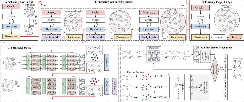
Figure 1: Overall framework of the PIL QAOA method for solving the MaxCut problem. The top parts a), b), and c) show the overview, while the bottom parts d) and e) show the design details of ”parameter reuse” and ”early break mechanism” in detail. a) Training the base graph which is randomly selected from the target graph, and the optimized parameters are obtained. b) The base graph is incremental by adding a portion of the remaining nodes and edges, and the initial parameters of the current phase are set as the optimized parameters of the previous phase. This part includes the ”parameter reuse” and ”early break mechanism”. c) Training the target graph to get the ultimate optimized parameters. d) The red arrow signifies the process of parameter reuse. e) When the currently optimized cut value is greater or equal to the maximum value of multiple random divisions, there is no need to wait for convergence. Then the next training phase is started, and the current optimized parameters are reused in the initial parameters of the next phase.

1. Proactively incremental learning: PIL QAOA is a method to solve optimization problems based on the idea of incremental learning. Taking the MaxCut problem as our example, a small subgraph (called base graph) is randomly selected from the whole graph (called target graph) in the first phase, and training the quantum circuit to get optimized parameters that imply its maximum cut. The MaxCut problem on the base graph is simpler to solve than that of the target graph. Then a portion of the remaining nodes and edges are added to the base graph to generate an incremental graph, and the circuit is retrained to get new optimized parameters. Next, in each subsequent phase, a portion of the remaining is further added to the incremental graph, and the circuit is retrained. The initial parameters of the current phase are reused from the optimized parameters in the previous phase. The adding, reusing, and retraining process continues until the MaxCut problem on the target graph is solved.

2. Early break mechanism: In order to further shorten the training time of the incremental phase, we design the ”early break” mechanism. When the optimized cut value is not less than the maximum cut value in k random partitions, the optimization of the next phase can be processed without waiting for convergence.

3. Extensive analysis of simulation experiments: To fully verify the performance of methods, we construct the MaxCut-Sandbox dataset. The dataset contains weighted graphs with three categories (random, regular, and complete), and unweighted graphs with three categories (random, regular, and complete). The number of nodes for each graph ranges from 5 to 10. The comparison experiment with existing QAOAs is composed of the performance on AR, training time, degree of anti-forgetting, and solving stability.

II Result

II.1 PIL QAOA

Most works of QAOA focus on the MaxCut problem, so PIL QAOA also elaborates on this problem. Existing works of QAOA usually directly train all nodes and edges of the graph when solving. The solution space tends to grow exponentially as the number of nodes increases. Solving in such a large solution space often results in poor performance. PIL QAOA adopts a progressive approach from a unique perspective, commencing with a smaller subgraph (called base graph) and expanding its scale gradually. Reusing previously optimized parameters by training to offer potent direction for subsequent incremental phases. The method implements an incremental way of training, which increases the performance. The overall framework process of PIL QAOA is illustrated in FIG. 1.

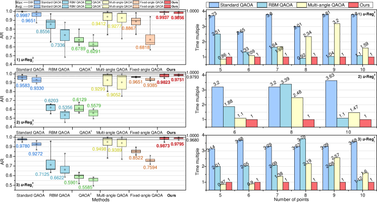
Figure 2: Comparison of AR and training time between the baseline methods and the proposed method in unweighted regular graphs. The left subfigure is the AR comparison, and the right subfigure is the training time comparison. In the left subfigure, each box is the overall AR values of the method in multiple graphs. The solid box and the dotted box represent the max and average distribution of AR in these graphs of the method. For example, in subfigure 1), the box corresponding to 0.9987 is the overall max AR of Standard QAOA on the $u\mathrm{-Reg}^{2}_{i}$ graphs ($i=5,6,7,8,9,10$), and the box corresponding to 0.9651 is the overall average AR of Standard QAOA on the $u\mathrm{-Reg}^{2}_{i}$ graphs ($i=5,6,7,8,9,10$). The horizontal axis represents different methods, and the vertical axis represents the AR value. The solid and dotted lines represent the max and average AR of GW. The specific number of each box is the average value of these ARs in multiple graphs. In the right subfigure, the specific number of each bar represents the training time multiple of the methods compared to PIL QAOA.

II.2 Comparison experiments on MaxCut

As mentioned in the Introduction, several quantum methods including Standard QAOA 10 , RBM QAOA 45 , $\mathrm{QAOA}^{2}$ 46 , Multi-angle QAOA 47 , and Fixed-angle QAOA 48 , have shown promising performance and offered valuable insights into the training of QAOA. Thus, this paper uses them as the baseline methods to conduct a comparison analysis with PIL QAOA proposed. Besides, GW 59 , as a representative classical algorithm, is also considered. We ”reproduce” these methods for selected problem instances and compare the AR and training time on six types of graphs (unweighted: regular, random, and complete graphs; weighted: regular, random, and complete graphs) with a 3-layers QAOA circuit. We give this difference in Time multiple $T_{x}/T_{ours}$, where $T_{x}$ represents the training time of various baseline methods, and $T_{ours}$ represents the complete time from selecting the base graph to completing the target graph optimization. Next, the stability of AR and the degree of anti-forgetting are compared. Furthermore, we also explore the selection of $p$-layers within the PIL QAOA method.

The comparison results in unweighted regular graphs and weighted random graphs are shown in the main paper, because regular graphs are commonly used in experiments of unweighted graphs 23 ; 24 ; 42 , and weighted random graphs are known for their complexity in solving. The comparison of other types of graphs (unweighted: random and complete graphs; weighted: regular and complete graphs) is shown in the Supplementary Information.

To ensure the fairness and reliability of our experiments, each experiment was repeated ten times for every instance, and the results were subsequently averaged to provide an evaluation.

II.2.1 Unweighted graphs

On unweighted regular graphs, FIG. 2 illustrates the AR and training time comparison between the baseline methods and PIL QAOA method. The experimental results on other types of unweighted graphs are shown in Supplementary information.

Table 1: Comparison of AR and training time between the baseline methods and the proposed method in unweighted regular graphs. Each experiment was repeated ten times for every graph, and the results were averaged to provide. Gray represents the performance of the classical GW method. Bold represents the best AR value of these QAOA methods.

AR (max)	$d=2$							$d=3$				$d=4$
	$i=5$	$i=6$	$i=7$	$i=8$	$i=9$	$i=10$	Avg ($i$)	$i=6$	$i=8$	$i=10$	Avg ($i$)	$i=5$	$i=6$	$i=7$	$i=8$	$i=9$	$i=10$	Avg ($i$)
GW (Classical)	1.0000	1.0000	1.0000	1.0000	1.0000	1.0000	1.0000	1.0000	1.0000	1.0000	1.0000	1.0000	1.0000	1.0000	1.0000	1.0000	1.0000	1.0000
Standard QAOA	1.0000	1.0000	1.0000	1.0000	0.9975	0.9947	0.9987	0.9943	0.9590	0.9215	0.9583	1.0000	0.9900	0.9860	0.9733	0.9486	0.9700	0.9780
RBM QAOA	0.9201	0.9734	0.9342	0.8451	0.8039	0.6570	0.8556	0.5512	0.6601	0.6496	0.6203	0.9575	0.6656	0.6750	0.7047	0.6389	0.6335	0.7125
$\mathrm{QAOA}^{2}$	0.8000	0.7000	0.6889	0.6328	0.6328	0.6187	0.6789	0.6786	0.5600	0.6000	0.6129	0.6282	0.6333	0.5625	0.5167	0.5982	0.6016	0.5901
Multi-angle QAOA	1.0000	1.0000	0.9977	0.9757	0.9358	0.7377	0.9412	0.9999	0.9867	0.8032	0.9299	1.0000	1.0000	0.9980	0.9843	0.9337	0.7830	0.9498
Fixed-angle QAOA	0.9277	0.9844	0.8658	0.9650	0.8349	0.7421	0.8867	0.9710	0.9655	0.9589	0.9651	0.8955	0.8725	0.8332	0.8206	0.8771	0.8141	0.8522
Ours	1.0000	0.9993	0.9957	1.0000	0.9970	0.9910	0.9972	0.9998	0.9960	0.9900	0.9953	1.0000	1.0000	0.9977	0.9961	0.9981	0.9851	0.9962
AR (avg)	$d=2$							$d=3$				$d=4$
	$i=5$	$i=6$	$i=7$	$i=8$	$i=9$	$i=10$	Avg ($i$)	$i=6$	$i=8$	$i=10$	Avg ($i$)	$i=5$	$i=6$	$i=7$	$i=8$	$i=9$	$i=10$	Avg ($i$)
GW (Classical)	1.0000	1.0000	1.0000	1.0000	1.0000	1.0000	1.0000	1.0000	0.9745	0.9634	0.9793	0.9733	0.9655	1.0000	0.9634	0.9335	0.9725	0.9680
Standard QAOA	0.9980	1.0000	0.9960	0.9780	0.9465	0.8720	0.9651	0.9806	0.9280	0.8905	0.9330	0.9293	0.9215	0.9624	0.9607	0.9206	0.8688	0.9272
RBM QAOA	0.8766	0.8371	0.8460	0.7462	0.4836	0.6118	0.7336	0.4540	0.5883	0.5644	0.5356	0.8304	0.5866	0.6074	0.6947	0.6316	0.6224	0.6622
$\mathrm{QAOA}^{2}$	0.7371	0.6587	0.6152	0.5725	0.6138	0.5770	0.6291	0.6063	0.4954	0.5719	0.5579	0.5749	0.5843	0.5438	0.4938	0.5812	0.5727	0.5585
Multi-angle QAOA	1.0000	1.0000	0.9966	0.9642	0.9131	0.6921	0.9277	0.9994	0.9674	0.7489	0.9052	1.0000	0.9999	0.9978	0.9748	0.8897	0.7711	0.9389
Fixed-angle QAOA	0.6997	0.5899	0.6605	0.941	0.6332	0.5662	0.6818	0.9622	0.9212	0.9321	0.9385	0.7733	0.8078	0.7537	0.7525	0.7191	0.7501	0.7594
Ours	0.9993	0.9985	0.9910	0.998	0.9860	0.9810	0.9923	0.9991	0.9872	0.9758	0.9874	1.0000	0.9977	0.9986	0.9857	0.9698	0.9791	0.9885
Time (second)	$d=2$							$d=3$				$d=4$
	$i=5$	$i=6$	$i=7$	$i=8$	$i=9$	$i=10$	Avg ($i$)	$i=6$	$i=8$	$i=10$	Avg ($i$)	$i=5$	$i=6$	$i=7$	$i=8$	$i=9$	$i=10$	Avg ($i$)
Standard QAOA	45.66	44.46	97.43	115.70	319.83	935.44	259.75	62.22	128.04	958.51	382.92	54.80	86.76	101.61	150.08	305.09	962.79	276.86
RBM QAOA	30.66	22.39	42.14	35.35	87.59	270.27	81.40	36.63	135.76	290.85	154.41	35.20	48.25	64.65	173.89	193.07	300.20	135.88
Multi-angle QAOA	10.46	18.24	43.14	90.00	268.84	391.49	137.03	21.35	99.40	387.25	169.33	15.18	21.26	42.71	100.67	238.30	429.64	141.29
Ours	12.23	16.78	25.66	38.38	83.98	246.09	70.52	19.46	40.04	264.01	107.84	17.47	23.56	30.93	45.96	92.73	268.98	79.94

Detailed experimental data can be found in TABLE 1. In terms of AR, we select complete baseline methods. In terms of training time, it should be noted that GW is a classical method, the parameters of Fixed-angle QAOA are determined and do not require further training, and $\mathrm{QAOA}^{2}$ is designed to solve the large-scale MaxCut problem, and its performance on the small-scale graphs is unsatisfactory. Therefore, in this training time comparison, we select the following baseline methods: Standard QAOA, RBM QAOA, and Multi-angle QAOA. It should be noted that each value is the average of 10 test results, and there is rounding.

According to the results in FIG. 2, TABLE 1, and Supplementary TABLE 4, Supplementary TABLE 5, we find that in terms of the AR of unweighted graphs:

1. For example, in the 3-regular graphs ($u\mathrm{-Reg}^{3}_{i}$), the ARs of PIL QAOA are higher by 37.5% (max) and 45.18% (avg) than those of RBM QAOA, and also outperform Fixed-angle QAOA by 3.02% (max) and 4.89% (avg). For all unweighted graphs, the ARs of PIL QAOA are higher by about 1.84% 43.24%(max) and 3.12%-43.24% (avg) than baseline methods.

2. For all unweighted graphs with less than 10 nodes, the ARs of PIL QAOA decrease relatively slightly as the number of nodes increases. Although Standard QAOA and Multi-angle QAOA perform well in graphs with fewer nodes, their efficiency drops significantly as the number of nodes increases. In contrast, PIL QAOA maintains relatively stable high performance even as the number of nodes increases. At the same time, PIL QAOA displays equivalent solution performance to that of the GW method and even exceeds it in certain cases.

In terms of training time of unweighted graphs:

1. PIL QAOA consistently has a shorter training time than the baseline methods in different graphs. For unweighted graphs, the training time of PIL QAOA is reduced by about 32.59% 64.82% compared to baseline methods. It can be seen that PIL QAOA greatly improves computational efficiency for various graphs.

II.2.2 Weighted graphs

On weighted random graphs, FIG. 3 illustrates the AR and training time comparison between the baselines and PIL QAOA method. The experimental results on other types of weighted graphs are shown in Supplementary information.

Detailed experimental data can be found in TABLE 2 It should be noted that Fixed-angle QAOA and Multi-angle QAOA are not suitable for solving weighted graphs, therefore other methods (GW, Standard QAOA, RBM QAOA, and $\mathrm{QAOA}^{2}$) are employed in this experiment. As for training time, similar to the experiments on unweighted graphs, here we don’t consider $\mathrm{QAOA}^{2}$ as well, and the selected baseline methods are Standard QAOA and RBM QAOA.

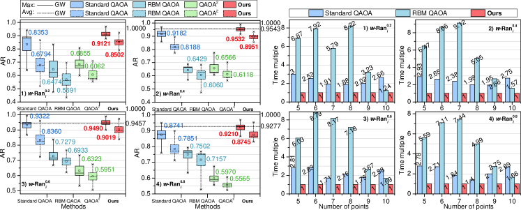
Figure 3: Comparison of AR and training time between the baseline methods and the proposed method in weighted random graphs. The left subfigure is the AR comparison, and the right subfigure is the Time comparison. Each box is the overall AR values of the method in multiple graphs. The solid box and the dotted box represent the max and average AR distribution of AR in these graphs of the method. The horizontal axis represents different methods, and the vertical axis represents the AR value. The solid and dotted lines represent the max and average AR of GW. The specific number of each box is the average value of these ARs in multiple graphs.

Table 2: Comparison of AR and training time between the baseline methods and the proposed method in weighted random graphs. Each experiment was repeated ten times for every graph, and the results were averaged to provide. Gray represents the performance of the classical GW method. Bold represents the best AR value of these QAOA methods.

AR (max)	$i=5$					$i=6$					$i=7$
	$ep=0.2$	$ep=0.4$	$ep=0.6$	$ep=0.8$	Avg ($ep$)	$ep=0.2$	$ep=0.4$	$ep=0.6$	$ep=0.8$	Avg ($ep$)	$ep=0.2$	$ep=0.4$	$ep=0.6$	$ep=0.8$	Avg ($ep$)
GW (Classical)	1.0000	1.0000	1.0000	1.0000	1.0000	1.0000	1.0000	1.0000	1.0000	1.0000	1.0000	1.0000	1.0000	1.0000	1.0000
Standard QAOA	0.9035	0.9700	0.9938	0.9135	0.9452	0.942	0.9667	0.9551	0.9496	0.9534	0.7452	0.8796	0.9338	0.7595	0.8295
RBM QAOA	0.8337	0.5964	0.7041	0.6333	0.6919	0.7956	0.6711	0.8381	0.7932	0.7745	0.7033	0.5686	0.6680	0.7598	0.6749
$\mathrm{QAOA}^{2}$	0.8077	0.7750	0.7031	0.5938	0.7199	0.7333	0.7083	0.7333	0.6750	0.7125	0.6735	0.6190	0.5903	0.5568	0.6099
Ours	0.9330	0.9899	0.9893	0.9447	0.9642	0.9687	0.9834	0.9710	0.9680	0.9728	0.8991	0.9472	0.9534	0.8651	0.9162
AR (max)	$i=8$					$i=9$					$i=10$
	$ep=0.2$	$ep=0.4$	$ep=0.6$	$ep=0.8$	Avg ($ep$)	$ep=0.2$	$ep=0.4$	$ep=0.6$	$ep=0.8$	Avg ($ep$)	$ep=0.2$	$ep=0.4$	$ep=0.6$	$ep=0.8$	Avg ($ep$)
GW (Classical)	1.0000	1.0000	1.0000	1.0000	1.0000	1.0000	1.0000	1.0000	1.0000	1.0000	1.0000	1.0000	1.0000	1.0000	1.0000
Standard QAOA	0.8809	0.8583	0.8977	0.8654	0.8756	0.6395	0.9424	0.9446	0.8807	0.8518	0.9005	0.8923	0.8684	0.8757	0.8842
RBM QAOA	0.5455	0.6689	0.6887	0.7570	0.6650	0.5306	0.6643	0.7398	0.7892	0.6810	0.4756	0.6882	0.7285	0.7684	0.6652
$\mathrm{QAOA}^{2}$	0.6000	0.6067	0.5333	0.5714	0.5779	0.6735	0.6058	0.6295	0.5956	0.6261	0.6250	0.6250	0.6042	0.5893	0.6109
Ours	0.8776	0.9155	0.9397	0.9389	0.9179	0.8823	0.9510	0.9402	0.8999	0.9184	0.9120	0.9321	0.9004	0.9096	0.9135
AR (avg)	$i=5$					$i=6$					$i=7$
	$ep=0.2$	$ep=0.4$	$ep=0.6$	$ep=0.8$	Avg ($ep$)	$ep=0.2$	$ep=0.4$	$ep=0.6$	$ep=0.8$	Avg ($ep$)	$ep=0.2$	$ep=0.4$	$ep=0.6$	$ep=0.8$	Avg ($ep$)
GW (Classical)	1.0000	0.9522	0.9465	0.9359	0.9587	1.0000	0.9564	0.9375	0.9216	0.9539	1.0000	0.9542	0.9475	0.9221	0.956
Standard QAOA	0.7644	0.8951	0.9603	0.7802	0.8500	0.8666	0.8346	0.8722	0.8979	0.8678	0.6495	0.8330	0.8167	0.7462	0.7614
RBM QAOA	0.6959	0.4738	0.6217	0.5282	0.5799	0.5874	0.6082	0.7676	0.7513	0.6786	0.6813	0.5613	0.6438	0.7375	0.6560
$\mathrm{QAOA}^{2}$	0.7095	0.7024	0.6745	0.5479	0.6586	0.6827	0.6611	0.6367	0.6068	0.6468	0.5758	0.5768	0.5839	0.5284	0.5662
Ours	0.8590	0.9248	0.9734	0.8673	0.9061	0.9223	0.9343	0.9386	0.9535	0.9372	0.8500	0.9160	0.9012	0.8306	0.8745
AR (avg)	$i=8$					$i=9$					$i=10$
	$ep=0.2$	$ep=0.4$	$ep=0.6$	$ep=0.8$	Avg ($ep$)	$ep=0.2$	$ep=0.4$	$ep=0.6$	$ep=0.8$	Avg ($ep$)	$ep=0.2$	$ep=0.4$	$ep=0.6$	$ep=0.8$	Avg ($ep$)
GW (Classical)	1.0000	0.9571	0.9467	0.9309	0.9587	1.0000	0.9553	0.9469	0.9228	0.9563	1.0000	0.9506	0.9471	0.9303	0.9570
Standard QAOA	0.5745	0.7737	0.8323	0.7642	0.7362	0.5194	0.8002	0.8105	0.7118	0.7105	0.7017	0.7764	0.7238	0.8102	0.7530
RBM QAOA	0.5326	0.6631	0.6807	0.7477	0.6560	0.4847	0.6461	0.7252	0.7681	0.6560	0.4329	0.6837	0.7208	0.7614	0.6497
$\mathrm{QAOA}^{2}$	0.5611	0.5638	0.5067	0.5241	0.5389	0.5533	0.5817	0.6000	0.5654	0.5751	0.5545	0.5852	0.5688	0.5661	0.5687
Ours	0.8090	0.8559	0.8912	0.8851	0.8603	0.7900	0.8630	0.8679	0.8479	0.8422	0.8711	0.8764	0.8390	0.8627	0.8623
Time (second)	$i=5$					$i=6$					$i=7$
	$ep=0.2$	$ep=0.4$	$ep=0.6$	$ep=0.8$	Avg ($ep$)	$ep=0.2$	$ep=0.4$	$ep=0.6$	$ep=0.8$	Avg ($ep$)	$ep=0.2$	$ep=0.4$	$ep=0.6$	$ep=0.8$	Avg ($ep$)
Standard QAOA	32.81	36.48	31.91	38.35	34.89	45.19	59.60	58.42	63.40	56.65	56.72	69.05	65.61	71.39	65.69
RBM QAOA	75.07	80.44	68.46	77.03	75.25	141.49	194.59	181.16	166.18	170.86	171.71	264.24	313.77	288.58	259.58
Ours	10.92	12.44	11.36	13.79	12.13	17.87	22.47	20.61	23.36	21.08	29.66	28.98	38.39	38.79	33.96
Time (second)	$i=8$					$i=9$					$i=10$
	$ep$=0.2	$ep$=0.4	$ep$=0.6	$ep$=0.8	Avg ($ep$)	$ep$=0.2	$ep$=0.4	$ep$=0.6	$ep$=0.8	Avg ($ep$)	$ep$=0.2	$ep$=0.4	$ep$=0.6	$ep$=0.8	Avg ($ep$)
Standard QAOA	86.48	97.25	103.65	102.09	97.37	244.41	285.41	263.30	279.31	268.11	913.76	957.67	913.62	979.61	941.17
RBM QAOA	379.10	247.61	345.10	365.40	334.30	390.49	391.19	401.87	383.94	391.87	426.46	547.22	599.90	605.11	544.67
Ours	46.12	49.07	48.09	73.18	54.11	121.00	146.16	150.73	139.38	139.32	344.01	348.39	354.67	364.00	352.77

According to the results in FIG. 3, TABLE 2, and Supplementary 6, Supplementary TABLE 7, we find that in terms of the AR of weighted graphs:

1. Compared with the baseline methods, PIL QAOA method shows superior performance on various weighted graphs. For example, for weighted random graphs, the ARs of PIL QAOA are higher by 29.10% (max) and 23.44% (avg) than those of $\mathrm{QAOA}^{2}$. For all weighted graphs, the ARs of PIL QAOA are higher by about 7.98% 31.42%(max) and 15.34%-30.2%(avg) than baseline methods.

2. For all weighted graphs with less than 10 nodes, the ARs of PIL QAOA decrease relatively slightly as the number of nodes increases. Meanwhile, in most scenarios, the ARs of PIL QAOA are typically equivalent to and can even surpass that of the GW classical method.

In terms of training time of weighted graphs:

1. PIL QAOA has a shorter training time than the baseline methods on various weighted graphs. For weighted graphs, the training time of PIL QAOA is reduced by 78.04% compared to Standard QAOA and by 74.07% compared to RBM QAOA.

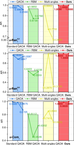
Figure 4: Comparison of the anti-forgetting degree of the baseline methods and the proposed method in the unweighted graphs. The diagram is shown in the lower left corner. Complete graphs and random graphs with edge probabilities of 0.2 and 0.8 are selected for experiments. The column represents the AR of the method on the old graphs (4 nodes), and the broken line shows the AR of applying the optimization parameters of the new graphs (with 6, 8, and 10 nodes) to solve the old graphs.

II.2.3 Degree of anti-forgetting

In the domain of machine learning, the forgetting problem has received widespread attention 60 ; 61 , which causes the model to compromise its performance on old datasets during the optimization process of new datasets. For the MaxCut problems, the performance decline of the model on the old graph after solving the new graph is called forgetting. PIL QAOA exhibits remarkable anti-forgetting abilities and effectively slows down catastrophic amnesia. To demonstrate this point, we compared the anti-forgetting properties of traditional methods and PIL QAOA. The relevant results are shown in FIG. 4.

By observing FIG. 4, we can find that in terms of the degree of anti-forgetting: PIL QAOA shows excellent anti-forgetting performance in different graphs. For example, in unweighted complete graphs, the ARs of PIL QAOA are higher by 25.90% (6 nodes), 13.60% (8 nodes), and 31.75% (10 nodes) than those of Multi-angle QAOA. This result demonstrates that PIL QAOA can effectively retain previously acquired knowledge when optimizing new graphs and will not significantly damage the performance of old graphs. This feature enhances its applicability in the fields of continuous learning and multi-task learning.

II.2.4 Performance stability

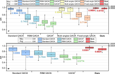
Figure 5: Comparison of AR stability between the baseline methods and the proposed method. The figures above and below represent the results of unweighted graphs and weighted graphs respectively. The rest of the legend information is the same as FIG. 2.

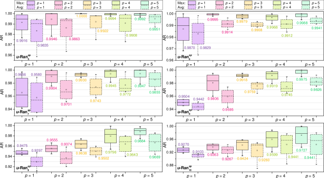
Figure 6: Comparison of AR stability between the baseline methods and the proposed method. The figures above and below represent the results of unweighted graphs and weighted graphs respectively. The rest of the legend information is the same as FIG. 2.

To ensure that algorithms are reliable and robust in practical applications, methods that show a high level of result stability are generally favored. So this paper conducts a comprehensive comparison of the performance stability of the baseline methods and PIL QAOA on various unweighted and weighted graphs, including random graphs with varying edge probabilities, regular graphs with different degrees of connectivity, and complete graphs. The relevant comparison results are detailed in FIG. 5. In this figure, the smaller the area of the box, the more stable the method is.

According to FIG. 5, PIL QAOA shows superior robustness and reliability compared with the baseline methods on various unweighted and weighted graphs.

II.2.5 Experiments with different $p$-layers

In the above simulation experiments, we fix the number of layers (denoted by $p$) to 3. There may be concerns about how to determine a proper $p$ and whether the performance will be enhanced with the $p$ increasing. Taking these into account,we compare the AR of PIL QAOA in unweighted graphs under varying $p$ (1-5). Here are the experimental results of random graphs with high complexity in FIG. 6. The experimental results of other types of graphs are shown in Supplementary information.

Based on the different $p$-layer experimental results presented in FIG. 6, Supplementary TABLE 8, Supplementary TABLE 9, and Supplementary TABLE 10, the following observations can be made for the unweighted graph:

1. In random graphs with fewer nodes, as $p$ increases, the stability of the AR increases. For example, when $i=5$, the upper and lower limits of the average AR gradually converge with the increase of the number of layers $p$.

2. For unweighted graphs, as the number of layers increases, the AR generally shows an increasing trend. However, the increase in the number of layers does not result in a significant improvement in the AR. Generally, a deeper level $p$ typically results in extended training durations. Hence, in our experiments, a smaller $p$ is more suitable.

For future research, especially research on larger graphs, the increase in the number of $p$ layers will help improve the approximation ratio of the overall solution, but the degree of improvement does not increase linearly. This inspires us that choosing a larger $p$ requires comprehensive consideration of the effect of the approximate ratio improvement and the cost of extending the training time.

II.2.6 Outlook

In this section, we delve into a novel and computationally intricate application: the incremental MaxCut problem. We further explore the inherent advantages of PIL QAOA in addressing such issues.

The incremental MaxCut is an ever-increasing scale MaxCut problem, commonly observed in real-world scenarios like the increase in the number of users in social networks 62 . As the size and topology of the graph grow, so does the complexity of deploying QAOA. Traditional QAOA methods often choose complete re-optimization when faced with the ever-expanding MaxCut. Admittedly, this strategy poses computational power challenges including the lengthy period of training time and the intensive computational resources. For example, when a 4-node MaxCut problem scales with new $n$ nodes and associated edges, standard techniques tend to re-optimize the entire graph that now contains $4+n$ nodes, thus amplifying the computational requirements.

Excitingly, we discover that our method can elegantly address these challenges. PIL QAOA shows obvious superiority in this regard and exhibits excellent performance when dealing with incremental problems. PIL QAOA can effectively learn optimized parameters for smaller graphs and apply them to parameter initialization for incremental graphs. Next, by fine-tuning these parameters, the performance of solving the MaxCut problem on incremental graphs is significantly improved. This method avoids unnecessary training time overhead and opens a new door for practical applications of optimization problems.

III Discussion

In this paper, a novel QAOA, called PIL QAOA, is proposed from a unique perspective to get a superior performance. We proactively transform the training way into an incremental learning approach. We transform the MaxCut problem solution for large graphs into a combination of small graph solutions and incremental learning step-by-step solutions. Although the training is divided into multiple phases, training on relatively simple subgraphs points the way to parameter initialization for large graph problems, thus achieving better performance. Experiments on the MaxCut-Sandbox datasets show that PIL QAOA exhibits superior AR, stability, and anti-forgetting, and significantly shortens the training time. In addition, we also explore the impact of different choices of $p$ in the AR, providing some reference for the design of future methods.

Notably, PIL QAOA hasn’t been tested on large-scale problems due to the limitation of simulating quantum computation via classical computers. The performance of our method on large-scale graphs remains an area that requires further validation in the future. Furthermore, besides the MaxCut problem investigated in this paper, exploring the application of the presented incremental method on other optimization problems is significant as well. Although PIL QAOA is a quantum algorithm, we hope the idea of converting problems into an incremental learning approach can also be applied in the future to optimize the solution process of classical algorithms, offering a fresh perspective for problem resolution.

IV Method

IV.1 Early break mechanism

In existing QAOA methods, the classic optimizer often terminates when the gradient convergence, resulting in unnecessary time overhead. We believe that the optimization parameters reused from the previous step allow us to reduce the solution scope of the incremental graphs. To enhance the efficiency of our parameters reuse strategy and decrease redundant optimization, we designed the early break mechanism in the incremental learning phases. This mechanism consists of two modules, i.e. the randomly solved module and the comparison module. The randomly solved module requires solving multiple times randomly and choosing the best solution as the output. The comparison module will compare the output of the randomly solved module to the current optimized solution. Training is stopped early if the current solution is greater or equal to the random solution. On the contrary, optimization will persist. Algorithm 1 shows the detailed steps of the proposed mechanism.

Algorithm 1 Early break mechanism of PIL QAOA.

1:Incremental graph $G^{\prime}$, current parameters $\psi$.

2:Initialize the early break value of Boolean variable “stop-optimize” to False, $C(z)$ and $C^{\prime}(z)$ to negative infinity;

3:for $i=1,2$, $\dots$, $k$ do:

4:     Randomly divide the incremental graph $G^{\prime}$ into node sets $V_{+}$ and $V_{-}$ multiple times to obtain the corresponding divided bit strings $z_{i}$;

5:     Calculate the cut value $C(z_{i})$ corresponding to $z_{i}$;

6:end for

7:Sort $C(z_{i})$ to get the maximum value $C(z)_{max}$;

8:From the current parameters $\psi$, $C^{\prime}(z)$ of the incremental graph $y$ is obtained;

9:if $C^{\prime}(z)\geq C(z)_{max}$ then:

10:     Set the stop-optimize value to True;

11:end if

12:if the stop-optimize value is True then:

13:     Jump out of the optimization process of the current incremental graph $G^{\prime}$ and enter the optimization process of the next incremental graph or target graph $G^{\prime\prime}$;

14:else

15:     Optimization of the currently incremental graph $G^{\prime}$ is continued;

16:end if

17:Repeat the above steps until entering the optimization process of the target graphs.

IV.2 Classic optimizer

In PIL QAOA, a classic optimizer is employed to optimize the graph’s parameters. Gradient descent algorithms can be used such as COBYLA (Constrained Optimization BY Linear Approximation) 63 ; 64 ; 65 , SLSQP (Sequential Least Squares Programming) 66 , BFGS (Broyden-Fletcher-Goldfarb-Shanno) 67 , and BOBYQA (Bound Optimization BY Quadratic Approximation) 68 ; 69 to achieve the convergence of cost values. In the experimental part, we choose the COBYLA algorithm, which is simple and has a good optimization effect.

IV.3 Experiments Settings

This section provides a comprehensive account of the experimental settings, including dataset construction, and evaluation metrics.

IV.3.1 Dataset construction

To assess the effectiveness of PIL QAOA in solving MaxCut problems, we construct a novel and comprehensive dataset called ”MaxCut-Sandbox” for QAOA. MaxCut-Sandbox consists of six graph types: unweighted: random, regular, and complete graphs; weighted: random, regular, and complete graphs. For the experiment, we set the number of nodes in the base graph to 4 and chose a range of 5 to 10 nodes for the target graph to observe AR. (Considering the performance constraints of computational simulation, the upper limit of the number of nodes is also selected to be about 10, which is selected in most experimental parts of existing work.) One node with corresponding edges is added to the subgraph in each phase. The specific information of the MaxCut-Sandbox is shown in TABLE 3.

Table 3: Specific information of the MaxCut-Sandbox.

Random	Number of nodes	Probability of edges	Symbol
	5, 6, 7, 8, 9, 10	0.2, 0.4, 0.6, 0.8	$x\mathrm{-Ran}_{i}^{ep}$
Regular	Number of nodes	Degree	Symbol
	5, 6, 7, 8, 9, 10	2
	6, 8, 10	3	$x\mathrm{-Reg}_{i}^{d}$
	5, 6, 7, 8, 9, 10	4
Complete	Number of nodes		Symbol
	5, 6, 7, 8, 9, 10		$x\mathrm{-Com}_{i}$

• Footnote: $x$ represents whether there is authority, $x={u,w}$, when $x$ is $u$, it is an unweighted graph; when $x$ is $w$, it is a weighted graph. $ep$ represents the probability of generating an edge, with $ep$={0.2, 0.4, 0.6, 0.8}. $i$ represents the number of nodes, $i=\{5,6,7,8,9,10\}$. $d$ represents the degree, with $d=\{2,3,4\}$. For example, $u\mathrm{-Ran}_{6}^{0.4}$ represents an unweighted random graph with 6 nodes with edge probability 0.4; $w\mathrm{-Reg}_{9}^{4}$ represents a weighted regular graph with 9 nodes of degree 4.

IV.3.2 Evaluation metrics

To evaluate the performance of the methods, we use AR as one of the key evaluation metrics 39 ; 40 ; 41 ; 42 . This index represents the ratio between the approximate solution $C_{A}$ obtained by the method and the actual optimal solution $C^{*}$ to the problem. Its formula is shown below:

$$\mathrm{AR}=\frac{C_{A}}{C^{*}},$$ (1)

The range of AR values is $[-1,1]$. The greater the absolute value of the AR value, the better the performance will be.

To eliminate the randomness of the optimization process as much as possible, we repeat each solution process 10 times, and calculate the maximum value and average value of these 10 occurrences.

Furthermore, we utilize T to evaluate the training time of the methods. Its formula is shown below:

$$\mathrm{T}=T_{end}-T_{start},$$ (2)

where, $T_{end}$ and $T_{start}$ represent the timestamp of ending training and starting training.

Reference

Graham, T. et al. Multi-qubit entanglement and algorithms on a neutral-atom quantum computer. Nature 604, 457-462 (2022).

Bartolucci, S., et al. Fusion-based quantum computation. Nat. Commun. 14, 912 (2023).

Stanisic, S. et al. Observing ground-state properties of the Fermi-Hubbard model using a scalable algorithm on a quantum computer. Nat. Commun. 13, 5743 (2022).

Preskill, J. Quantum computing in the NISQ era and beyond. Quantum 2, 79 (2018).

Sivarajah, S. et al. t—ket⟩: a retargetable compiler for NISQ devices. Quantum Sci. Technol. 6, 014003 (2020).

Zhang, S. X. et al. Tensorcircuit: a quantum software framework for the nisq era. Quantum 7, 912 (2023).

Kokail, C. et al. Self-verifying variational quantum simulation of lattice models. Nature 569, 355-360 (2019).

Antol, S. et al. Vqa: Visual question answering. In Proceedings of the IEEE international conference on computer vision(ICCV), 2425-2433 (2015).

Goyal, Y., Khot, T., Summers-Stay, D., Batra, D., & Parikh, D. Making the v in vqa matter: Elevating the role of image understanding in visual question answering. In Proceedings of the IEEE conference on computer vision and pattern recognition(CVPR), 6904-6913 (2017).

Chandarana, P. et al. Digitized-counterdiabatic quantum approximate optimization algorithm. Phys. Rev. Res. 4, 013141 (2022).

Chancellor, N. Domain wall encoding of discrete variables for quantum annealing and QAOA. Quantum Sci. Technol. 4, 045004 (2019).

Anshu, A. & Metger, T. Concentration bounds for quantum states and limitations on the QAOA from polynomial approximations. Quantum 7, 999 (2023).

Zhu, Y. et al. Multi-round QAOA and advanced mixers on a trapped-ion quantum computer. Quantum Sci. Technol. 8, 015007 (2022).

Zhang, Y., Zhang, R. & Potter, A. C. QED driven QAOA for network-flow optimization. Quantum 5, 510 (2021).

Shaydulin, R., Alexeev, Y. Evaluating quantum approximate optimization algorithm: A case study. In Proceedings of the 2019 tenth international green and sustainable computing conference (IGSC),, 1-6 (2019).

Sharma, V., et al. Preprint at http://arXiv.org/abs/2210.08695 (2022). OpenQAOA–An SDK for QAOA. Preprint at http://arXiv.org/abs/2210.08695 (2022).

Farhi, E., Goldstone, J. & Gutmann S. A quantum approximate optimization algorithm. Preprint at https://arxiv.org/abs/1411.4028 (2014).

Farhi, E., Goldstone, J. & Gutmann, S. A quantum approximate optimization algorithm applied to a bounded occurrence constraint problem. Preprint at https://arxiv.org/abs/1412.6062 (2015).

Streif, M., Yarkoni, S., Skolik, A., Neukart, F., & Leib, M. Beating classical heuristics for the binary paint shop problem with the quantum approximate optimization algorithm. Phys. Rev. A 104, 012403 (2021).

Harrigan, M. P. et al. Quantum approximate optimization of non-planar graph problems on a planar superconducting processor. Nature Phys. 17, 332-336 (2021).

Anschuetz, E. R., & Kiani, B. T. Quantum variational algorithms are swamped with traps. Nat. Commun. 13, 7760 (2022).

Hashim, A. et al. Optimized SWAP networks with equivalent circuit averaging for QAOA. Phys. Rev. Res. 4, 033028 (2022).

Farhi, E., Goldstone, J., Gutmann, S., Zhou, L. The quantum approximate optimization algorithm and the Sherrington-Kirkpatrick model at infinite size. Quantum 6, 759 (2022).

Lykov, D., et al. Sampling frequency thresholds for the quantum advantage of the quantum approximate optimization algorithm. npj Quantum Inf. 9, 73 (2023). Sampling frequency thresholds for the quantum advantage of the quantum approximate optimization algorithm. npj Quantum Inf. 9, 73 (2023).

Ebadi, S. et al. Quantum optimization of maximum independent set using Rydberg atom arrays. Science 376, 209–1215 (2022).

Brady, L. T. et al. Optimal protocols in quantum annealing and quantum approximate optimization algorithm problems. Phys. Rev. Lett. 126, 070505 (2021). Optimal protocols in quantum annealing and quantum approximate optimization algorithm problems. Phys. Rev. Lett. 126, 070505 (2021).

Khairy, S., Shaydulin, R., Cincio, L., Alexeev, Y., & Balaprakash, P. Learning to Optimize Variational Quantum Circuits to Solve Combinatorial Problems. In Proceedings of the AAAI conference on artificial intelligence 34, 2367-2375 (2020).

Jain, N. et al. Graph neural network initialisation of quantum approximate optimisation. Quantum 6, 861 (2022).

Song, Y. et al. Trainability Analysis of Quantum Optimization Algorithms from a Bayesian Lens. Preprint at https://arxiv.org/abs/2310.06270 (2023).

Shaydulin, R., Lotshaw, P. C., Larson, J., Ostrowski, J. & Humble, T. S. Parameter transfer for quantum approximate optimization of weighted maxcut. ACM Trans. Quantum Comput. 4, 1-15 (2023).

Larkin, J. et al. Evaluation of QAOA based on the approximation ratio of individual samples. Quantum Sci. Technol. 7, 045014 (2022).

Sack, S. H., & Serbyn, M. Quantum annealing initialization of the quantum approximate optimization algorithm. Quantum 5, 491 (2021).

Egger, D. J., Mareček, J., & Woerner, S. Warm-starting quantum optimization. Quantum 5, 479 (2021).

Zhou, L. et al. Quantum approximate optimization algorithm: Performance, mechanism, and implementation on near-term devices. Phys. Rev. X 10, 021067 (2020).

Bravyi, S. et al. Obstacles to Variational Quantum Optimization from Symmetry Protection. Phys. Rev. Lett. 125, 260505 (2020).

Bravyi, S., Kliesch, A., Koenig, R., & Tang, E. Hybrid quantum-classical algorithms for approximate graph coloring. Quantum 6, 678 (2022).

Magann, A. B. et al. Feedback Based Quantum Optimization. Phys. Rev. Lett. 129, 250502 (2022).

Moussa, C., Wang, H., Bäck, T., & Dunjko, V. Unsupervised strategies for identifying optimal parameters in Quantum Approximate Optimization Algorithm. PJ Quantum Technol. 9, 11 (2022).

Streif, M., & Leib, M. Training the quantum approximate optimization algorithm without access to a quantum processing unit. Quantum Sci. Technol. 5, 34008 (2020).

Bonet-Monroig, X. et al. Performance comparison of optimization methods on variational quantum algorithms. Phys. Rev. A 107, 032407 (2023).

Hadfield, S., Hogg, T. & Rieffel, E. G. Analytical framework for quantum alternating operator ansatz. Quantum Sci. Technol. 8, 015017 (2022).

Karamlou, A. H. et al. Analyzing the performance of variational quantum factoring on a superconducting quantum processor. npj Quantum Inf. 7, 156 (2021).

Du, Y., Huang, T., You, S., Hsieh, M. H., & Tao, D. Quantum circuit architecture search for variational quantum algorithms. npj Quantum Inf. 8, 62 (2022).

Zhu, L., et al. Adaptive quantum approximate optimization algorithm for solving combinatorial problems on a quantum computer. Phys. Rev. Res. 4, 033029 (2022).

Medvidović, M. & Carleo, G. Classical variational simulation of the quantum approximate optimization algorithm. npj Quantum Inf. 7, 101 (2021).

Zhou, Z. et al. QAOA-in-QAOA: solving large-scale MaxCut problems on small quantum machines. Phys. Rev. Applied 19, 024027 (2023).

Herrman, R. et al. Multi-angle quantum approximate optimization algorithm. Sci. Rep. 12, 6781 (2022). Multi-angle quantum approximate optimization algorithm. Sci. Rep. 12, 6781 (2022).

Wurtz, J. & Lykov, D. Fixed-angle conjectures for the quantum approximate optimization algorithm on regular MaxCut graphs. Phys. Rev. A 104, 052419 (2021).

Wurtz, J. & Love, P. MaxCut quantum approximate optimization algorithm performance guarantees for p¿ 1. Phys. Rev. A 103, 042612 (2021).

Marwaha, K. Local classical MAX-CUT algorithm outperforms p= 2 QAOA on high-girth regular graphs. Quantum 5, 437 (2021).

Wang, Z. et al. Quantum approximate optimization algorithm for MaxCut: A fermionic view. Phys. Rev. A 97, 22304 (2018).

Wu, Y. et al. Large scale incremental learning. In Proceedings of the IEEE conference on computer vision and pattern recognition(CVPR), 374-382 (2019).

Castro, F. M., Marín-Jiménez, M. J., Guil, N., Schmid, C., & Alahari, K. End-to-end incremental learning. In Proceedings of the European conference on computer vision (ECCV), 233-248 (2018).

van de Ven, G. M., Tuytelaars, T., & Tolias, A. S. Three types of incremental learning. Nat. Mach. Intell. 4, 1185-1197 (2022).

Vandenhaute, S., Cools-Ceuppens, M., DeKeyser, S., Verstraelen, T., & Van Speybroeck, V. Machine learning potentials for metal-organic frameworks using an incremental learning approach. npj Comput. Mater. 9, 1-8 (2023).

Dong, N., Zhang, Y., Ding, M., & Lee, G. H. Incremental-DETR: Incremental few-shot object detection via self-supervised learning. In Proceedings of the AAAI Conference on Artificial Intelligence, 543-551 (2023).

Tadros, T., Krishnan, G. P., Ramyaa, R., & Bazhenov, M. Sleep-like unsupervised replay reduces catastrophic forgetting in artificial neural networks Nat. Commun. 13, 7742 (2022).

Dhapola, P. et al. Scarf enables a highly memory-efficient analysis of large-scale single-cell genomics data. Nat. Commun. 13, 4616 (2022).

Aryasetiawan, F., & Gunnarsson, O. The GW method. Rep. Prog. Phys. 61, 237 (1998).

Liu, H. et al. Overcoming catastrophic forgetting in graph neural networks. In Proceedings of the AAAI Conference on Artificial Intelligence 35, 8653-8661 (2021).

Kirkpatrick, J. et al. Overcoming catastrophic forgetting in neural networks. Proceedings of the national academy of sciences 114, 3521-3526 (2017).

Chierichetti, F. et al. On compressing social networks. In Proceedings of the 15th ACM SIGKDD international conference on Knowledge discovery and data mining (KDD), 219-228 (2009).

Fernández-Pendás, M. et al. A study of the performance of classical minimizers in the Quantum Approximate Optimization Algorithm. J. Comput. Appl. Math. 404, 113388 (2022).

Pellow-Jarman, A. et al. A comparison of various classical optimizers for a variational quantum linear solver. Quantum Inf. Process. 20, 202 (2021).

Cheng, L., Chen, Y. Q., Zhang, S. X., & Zhang, S. Error-mitigated Quantum Approximate Optimization via Learning-based Adaptive Optimization. Preprint at https://arxiv.org/abs/2303.14877 (2023).

Bonet-Monroig, X. et al. Performance comparison of optimization methods on variational quantum algorithms. Phys. Rev. A 107, 032407 (2023).

Lotshaw, P. C. et al. Empirical performance bounds for quantum approximate optimization. Quantum Inf. Process. 20, 1-32 (2021).

Sung, K. J. et al. Using models to improve optimizers for variational quantum algorithms. Quantum Sci. Technol. 5, 044008 (2020).

Shaydulin, R., Safro, I. & Larson, J. Multistart Methods for Quantum Approximate optimization. In Proceedings of the 2019 IEEE High Performance Extreme Computing Conference (HPEC), 1-8 (2019).