Predicting Ground Reaction Force from Inertial Sensors

Abstract

Machine learning methods can help overcome the difficulty and cost of data collection by predicting a signal of interest from other signals that can be collected more easily and with less expensive instrumentation. One example where this approach is crucial is the study of ground reaction force (GRF), which is used to characterize the mechanical loading experienced by individuals in movements such as running. An example clinical application is using GRF measures to identify athletes at risk for stress-related injuries. While direct measurement of GRF is possible with the use of instrumented treadmills in laboratories or force plates embedded into training environments, the ability to measure GRF during an entire outdoor run is not feasible. Our aim in this paper is to determine if data collected with inertial measurement units (IMUs), that can be worn by athletes during outdoor runs, can be used to predict GRF with sufficient accuracy to allow the analysis of its derived biomechanical variables (e.g., contact time, net vertical impulse, and loading rate).

In this paper, we consider lightweight approaches in contrast to state-of-the-art prediction using LSTM neural networks. Specifically, we compare use of LSTMs to $k$-Nearest Neighbors (KNN) regression as well as propose a novel solution, SVD Embedding Regression (SER), using linear regression between singular value decomposition embeddings of IMUs data (input) and GRF data (output). We evaluate the accuracy of these techniques when using training data collected from different athletes, from the same athlete, or both, and we explore the use of acceleration and angular velocity data from sensors at different locations (sacrum, left shank, and right shank). Our results illustrate that simple machine learning methods such as SER and KNN can be similarly accurate or more accurate than LSTM neural networks, with much faster training times and hyperparameter optimization; in particular, SER and KNN are more accurate when personal training data are available, and KNN comes with benefit of providing provenance of prediction. Notably, the use of personal data reduces prediction errors of all methods for most biomechanical variables.

[inst1]organization=University of Southern California, addressline=941 Bloom Walk, city=Los Angeles, postcode=90089, state=CA, country=USA

[inst2]organization=Columbia University, addressline=1214 Amsterdam Avenue, city=New York, postcode=10027, state=NY, country=USA

[inst3]organization=Massachusetts Institute of Technology, addressline=32 Vassar Street, city=Cambridge, postcode=02139, state=MA, country=USA

1 Introduction

Ground reaction force (GRF), the force exerted by the ground during contact with a body, is a measure that provides insight into the whole body dynamics of human movement in the field of biomechanics, characterizing mechanical loading of the body which contribute to stress-responses of bone and soft tissue. [1] Analysis of GRFs has been proposed as a mechanism for identifying factors that lead to bone stress injuries for runners. [2, 3, 4] To this end, domain experts analyze either the GRF waveform or discrete biomechanical variables derived from it, such as contact time, net vertical impulse, and loading rate [5, 6, 7, 8].

Direct measurement of GRF is typically performed using force plates or instrumented treadmills in a laboratory environment [9, 10, 11]; wearable GRF sensors have been proposed [12] but are not generally available. Machine learning methods can mitigate the challenges and costs associated with direct data collection by predicting signals of interest from other signals more readily accessible and from cost-effective sources. For ground reaction force, previous works [13, 14] address this problem by predicting GRF from acceleration and angular velocity waveforms collected using low-cost inertial measurement units (IMUs) that athletes can wear when running or during competition. State-of-the-art methods [14] that use LSTM neural networks to predict GRF waveforms from acceleration data present two major limitations: (1) long training times and hyperparameter optimization are required by neural networks; (2) predictions lack provenance and are challenging to explain based on historical examples.

In this work, we address these limitations by exploring lightweight alternatives to deep-learning methods to facilitate training and inference on devices with limited computing power, while also analyzing the improvements resulting from the use of training data collected for the target athletes at multiple body locations. Specifically, we compare state-of-the-art approaches based on LSTM neural networks with two lightweight approaches: SVD Embedding Regression (SER), our proposed approach to predict GRF through linear regression between singular value decomposition (SVD) embeddings of IMU data (input) and GRF data (output); and $k$-Nearest Neighbors (KNN) regression. We evaluate the accuracy of these techniques in predicting GRF and derived biomechanical variables when using training data collected (1) from different athletes, (2) from the same athlete, (3) or both. In each scenario, we explore the use of acceleration and angular velocity data from sensors positioned at different locations (sacrum, left and right shanks which are right above the left and right lateral malleolus). This data can be easily collected given the wide availability of wearable IMUs measuring linear acceleration, angular velocity, and magnetic fields concurrently.

To evaluate the efficacy of different machine learning methods under a variety of scenarios and input sensors, we use an existing set of deidentified data collected by domain experts working with Pac-12 conference collegiate distance runners. Details on the data collection and preprocessing are described in Section 2, while the different prediction tasks and metrics are defined in Section 3.

Our work provides the following contributions.

1. We propose SER, a novel approach to predict GRF from IMU measurements (Section 4.1), as an alternative to KNN (Section 4.2) and LSTM neural networks (Section 4.3).

2. Through our experimental results (Section 5), we show that simple machine learning methods such as SER and KNN can be similarly accurate or more accurate than LSTM neural networks, requiring fewer computing resources and energy, while allowing much faster training times and hyperparameter optimization.

3. We show that angular velocity measurements (collected by IMU sensors) improve GRF prediction accuracy when combined with acceleration measurements.

4. We illustrate how GRF from an individual athlete can significantly improve prediction accuracy, especially when KNN is used. When only personal training data is used, SER provides very accurate results, while LSTM neural networks are most accurate when using training data from other athletes (the setting considered by related work).

Notably, we achieve with this dataset better accuracy than state-of-the-art methods presented in the literature. The error in the predicted GRF waveform is sufficiently low to obtain accurate estimates of discrete biomechanical variables (e.g., contact time, net vertical impulse, active peak, loading rate).

2 Notation and Dataset

We use an existing Pac-12 dataset consisting of 44 competitive collegiate runners (25 female and 19 male) from University of Colorado Boulder, University of Oregon, and Stanford University in accordance with the Institutional Review Board for research involving human participants. (A subset of this dataset is used in [15, 16]). The dataset includes 78 collections (1–6 per participant) where participants ran on instrumented treadmills at multiple speeds: male participants ran at 7, 6.5, and 5 min/mi (3.8, 4.1, 5.4 m/s) and female participants ran at 7 and 5.5 min/mi (3.8, 4.9 m/s); GRF data was collected by the treadmills at 1,000 Hz, while wearable IMU sensors collected acceleration and angular velocity at the sacrum, left shank, and right shank with 500 Hz frequency. Including all athletes, collections, and running speeds, the dataset provides 276 running measurements, each with at least 60 steps (approximately 15 seconds). Examples of our collected signals are shown in Fig. 1.

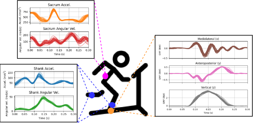
Figure 1: Locations and examples of running step signals from different sensors

We synchronize data events from different sensors, each measurement is split into individual foot contacts, and we reduce noise typically present in IMU and GRF data, similarly to related work [14], by applying a 4th order Butterworth low-pass filter with cut-off frequency of 20 Hz for acceleration and angular velocity signals, and 30 Hz for GRF signals. Applying the same filters allows us to make a fair quantitative comparison with related work. A detailed description of data preprocessing is provided in Appendix B.

After these operations, the dataset includes over 16,000 steps (either left or right), each with 5 discrete-time signals: acceleration $\vec{a}_{s}(t),\vec{a}_{lr}(t)$ and angular velocity $\vec{\omega}_{s}(t),\vec{\omega}_{lr}(t)$ at the sacrum ($s$) and left/right shanks ($lr$), respectively, and GRF $\vec{g}(t)$. Each signal includes $T=200$ time points (500 Hz frequency over a 400 ms time window) and 3 samples per time point $t=1,\dots,T$ (the mediolateral, anterior-posterior, and vertical components, respectively indicated as $x$, $y$, $z$).

3 Prediction Tasks and Metrics

3.1 Prediction Tasks and Hyperparameter Selection

We consider different scenarios for the prediction of GRF data: first, similarly to related work [14], we predict GRF of a target athlete using training data collected only from other athletes (we refer to this scenario as “others”); then, we consider scenarios where training data from the target athlete is used exclusively (scenario “personal”) or in conjunction with data from other athletes (scenario “everyone”).

For each scenario, we consider the use of the L2 norm (i.e., the magnitude) of different input signals to predict GRF: all acceleration and angular velocity signals $\lVert\vec{a}_{s}(t)\rVert,\lVert\vec{a}_{lr}(t)\rVert,\lVert\vec{\omega}_{s}(t)\rVert,\lVert\vec{\omega}_{lr}(t)\rVert$ (case “all”); only acceleration signals $\lVert\vec{a}_{s}(t)\rVert,\lVert\vec{a}_{lr}(t)\rVert$ (case “acc”) or only angular velocity signals $\lVert\vec{\omega}_{s}(t)\rVert,\lVert\vec{\omega}_{lr}(t)\rVert$ (case “ang”); both acceleration and angular velocity but only from sensors at the sacrum ($\lVert\vec{a}_{s}(t)\rVert,\lVert\vec{\omega}_{s}(t)\rVert$, case “sacrum”) or at the left and right shanks ($\lVert\vec{a}_{lr}(t)\rVert,\lVert\vec{\omega}_{lr}(t)\rVert$, case “shanks”). Finally, we consider using only the acceleration at the sacrum, either as a multidimensional signal $\vec{a}_{s}(t)$ (case “sac/acc3d”), or through its L2 norm $\lVert\vec{a}_{s}(t)\rVert$ (case “sac/acc”).

Scenarios, input signals, and machine learning methods are used to define prediction tasks, each identified by a tuple $(\textit{scenario},\textit{sensors},\textit{method})$ with $\textit{scenario}\in\{\textsc{others},\textsc{personal},\textsc{everyone}\}$, $\textit{sensors}\in\{\textsc{all},\textsc{acc},\textsc{ang},\textsc{sacrum},\textsc{shanks},\textsc{sac/acc3d},\textsc{sac/acc}\}$, and $\textit{method}\in\{\textsc{ser},\textsc{knn},\textsc{lstm}\}$. To select hyperparameters for each prediction task (e.g., the number of neighbors in knn or the model architecture of lstm), we repeat training 5 times, each time leaving out the data of an entire collection as validation set (with multiple running paces for a specific athlete). In the others scenario, when a collection is used for validation, the other collections of the same athlete are removed from the training set. After selecting hyperparameters with best average accuracy on the validation set, models are trained using the entire training set.

3.2 Error Metrics for Predicted GRF Waveforms

The proposed machine learning methods predict, for each step, the components of the GRF $\vec{g}(t)=\big{(}g_{x}(t),g_{y}(t),g_{z}(t)\big{)}$ at each time point $t=1,\dots,T$. We indicate the predictions by $\hat{g}_{x}(t)$, $\hat{g}_{y}(t)$, and $\hat{g}_{z}(t)$, respectively, and we evaluate the Root Mean Squared Error (RMSE) and the Relative Root Mean Squared Error (rRMSE) for each component $d\in\{x,y,z\}$:

$$RMSE(g_{d},\hat{g}_{d}) =\sqrt{\frac{\sum_{t=1}^{T}[g_{d}(t)-\hat{g}_{d}(t)]^{2}}{T}}$$ (1)

$$rRMSE(g_{d},\hat{g}_{d}) =\frac{RMSE(g_{d},\hat{g}_{d})}{[\textsc{range}(g_{d})+\textsc{range}(\hat{g}_{d})]/2}$$ (2)

where $\textsc{range}(v)=\max_{t=1,\dots,T}v(t)-\min_{t=1,\dots,T}v(t)$. We compute the average of these error metrics across predicted steps; related works consider GRF predictions to be very accurate when $RMSE(g_{z},\hat{g}_{z})<0.21$ [13] and $rRMSE(g_{z},\hat{g}_{z})<14\%$ [17]. Note that GRF is normalized by body weight in our dataset; even when omitted, RMSE errors are relative to body weights of the athletes.

3.3 Error Metrics for Predicted Biomechanical Variables

GRF waveforms are frequently used by domain experts to calculate scalar biomechanical variables representing different characteristics of a running step. We consider the biomechanical variables Loading Rate, Contact Time, Braking Time, Braking Percentage, Active Peak, Average Vertical Force, Vertical Impulse, and A/P Velocity Change (defined in  [1] and Appendix A). We evaluate each biomechanical variable $f$ from the predicted GRF waveform $\hat{g}_{x}(t),\hat{g}_{y}(t),\hat{g}_{z}(t)$ and from its actual value $g_{x}(t),g_{y}(t),g_{z}(t)$ for $t=1,\dots,T$, and we compute the mean absolute percentage error (MAPE), i.e., the mean of $|f(\hat{g}_{x},\hat{g}_{y},\hat{g}_{z})-f(g_{x},g_{y},g_{z})|/|f(g_{x},g_{y},g_{z})|$ across different steps. In addition to these metrics, we also study the effects of different prediction models on the resulting waveforms and their interpretability in Section 5.

4 Methods

4.1 SVD Embedding Regression (SER)

As a lightweight alternative to deep learning methods for the prediction of GRF from IMU signals (acceleration and angular velocity at different body locations), we propose the use of linear regression between SVD embeddings of input (IMU) and output (GRF) data; to reconstruct the GRF signals from the predicted output embedding (the pre-image problem), we use the right singular vectors of the training data. This approach (which can be viewed as a natural generalization of Principal Component Regression at a high dimension [18]) is similar to transduction of structured data [19], but pre-image calculation is very fast, providing a lightweight alternative to deep learning methods.

4.1.1 SVD Embedding of IMU and GRF Signals

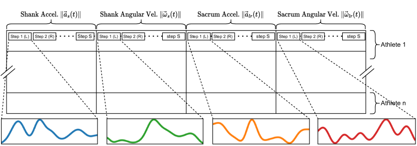
(a) $A_{IMU}$

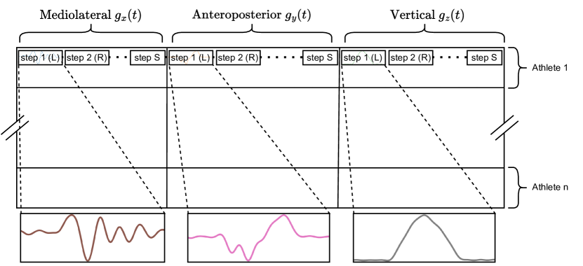
(b) $A_{GRF}$

Figure 2: Matrix Arrangements

We organize our training data into two matrices, $A_{IMU}$ Fig. 2(a) and $A_{GRF}$ Fig. 2(b). Each row of these matrices corresponds to a different batch of $S$ consecutive running foot contacts from a measurement (i.e., steps of an athlete running at a given speed); for each running step in a batch and time point $t$ (200 per step), the columns of $A_{IMU}$ include the IMU signals (e.g., the L2 norm of acceleration and angular velocity signals $\lVert\vec{a}_{s}(t)\rVert,\lVert\vec{a}_{lr}(t)\rVert,\lVert\vec{\omega}_{s}(t)\rVert,\lVert\vec{\omega}_{lr}(t)\rVert$ in the all case), while the columns of $A_{GRF}$ include the components of the GRF, i.e., $g_{x}(t),g_{y}(t),g_{z}(t)$.

To obtain low-dimensional embeddings of the training data, we compute the SVD decomposition of the matrices $A_{IMU}\in\mathbb{R}^{n\times m}$ and $A_{GRF}\in\mathbb{R}^{n\times p}$, i.e.,

$$\begin{split}A_{IMU}&=U_{IMU}\Sigma_{IMU}V_{IMU}^{T}\\ A_{GRF}&=U_{GRF}\Sigma_{GRF}V_{GRF}^{T}\end{split}$$ (3)

where: $U_{IMU}\in\mathbb{R}^{n\times n}$ and $U_{GRF}\in\mathbb{R}^{n\times n}$ are orthogonal matrices (with left singular vectors as columns); $\Sigma_{IMU}\in\mathbb{R}^{n\times m}$ and $\Sigma_{GRF}\in\mathbb{R}^{n\times p}$ are rectangular diagonal matrices (with singular values in ascending order on the diagonal); $V_{IMU}\in\mathbb{R}^{m\times m}$ and $V_{GRF}\in\mathbb{R}^{p\times p}$ are orthogonal matrices (with right singular vectors as columns).

We obtain low-rank approximations by keeping only the first $r$ singular values of the SVD decomposition, i.e., the first $r$ columns of the $U$ and $V$ matrices, and the first $r$ rows/columns of $\Sigma$:

$$\begin{split}A_{IMU}&\approx\overline{U}_{IMU}\overline{\Sigma}_{IMU}\overline{V}_{IMU}^{T}\\ A_{GRF}&\approx\overline{U}_{GRF}\overline{\Sigma}_{GRF}\overline{V}_{GRF}^{T}\end{split}$$ (4)

with $\overline{U}_{IMU}\in\mathbb{R}^{n\times r_{IMU}}$, $\overline{\Sigma}_{IMU}\in\mathbb{R}^{r_{IMU}\times r_{IMU}}$, $\overline{V}_{IMU}\in\mathbb{R}^{m\times r_{IMU}}$ and $\overline{U}_{GRF}\in\mathbb{R}^{n\times r_{GRF}}$, $\overline{\Sigma}_{GRF}\in\mathbb{R}^{r_{GRF}\times r_{GRF}}$, $\overline{V}_{GRF}\in\mathbb{R}^{p\times r_{GRF}}$. On our dataset, we use ranks $r_{IMU}=r_{GRF}=6$, which retain at least $95\%$ of the energy of $\Sigma_{IMU}$ and $\Sigma_{GRF}$, respectively (i.e., the sum of the squares of the retained singular values is at least $95\%$ of the sum of the squares of all the singular values). The rank 6 approximation of GRF has an average RMSE of 0.079 or rRMSE of 0.021; the same accumulative energy is also chosen in the literature [20, 21]. We also select the number of steps per row $S\in\{2,3,5,6,10,12,15,20,30,60\}$, using a validation set. Larger ranks $r_{IMU}$ and $r_{GRF}$ work similarly well, while the method is sensitive to $S$, as illustrated in Fig. 4.

4.1.2 Training and Prediction using SVD Embeddings

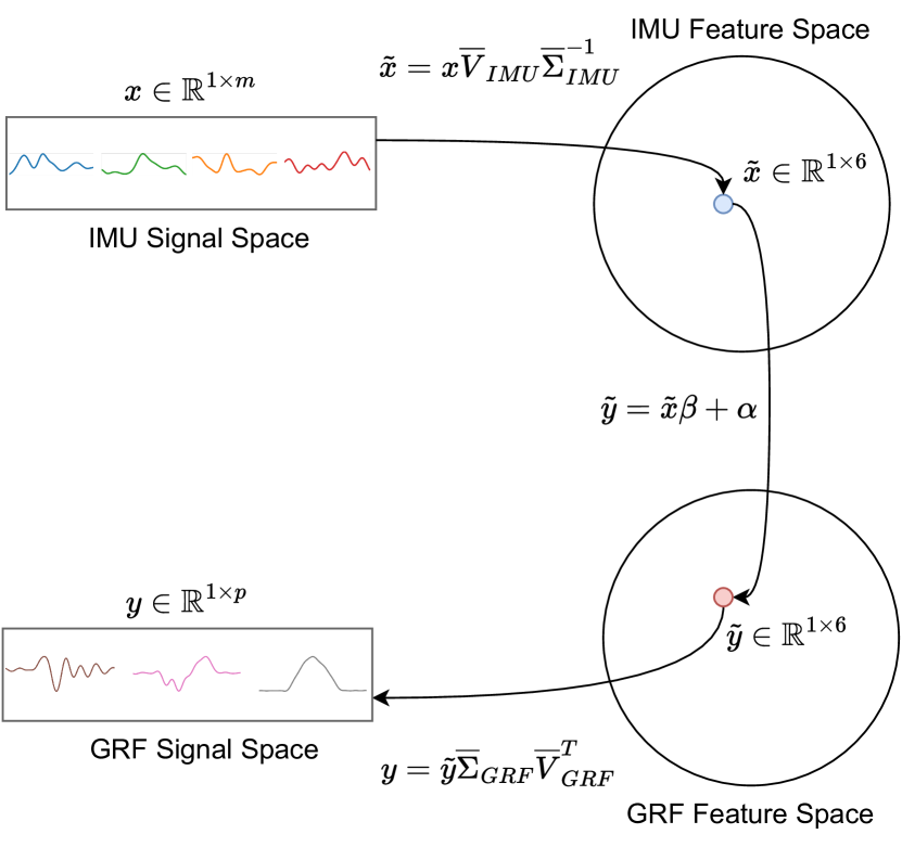
Figure 3: Predicting GRF with SVD-based output-Embedding Regression

After low-rank approximation, each row of matrices $\overline{U}_{IMU}$ and $\overline{U}_{GRF}$ is a vector with $r_{IMU}$ and $r_{GRF}$ components representing the embeddings (i.e., the features) of IMU (input) and GRF (output) signals, respectively, for a batch of $S$ running steps in the training set. We train a predictor for each component of the GRF embedding using least squares regression with elastic net regularization, i.e., we select, for each $j=1,\dots,r_{GRF}$, the parameters $\beta_{j}\in\mathbb{R}^{r_{IMU}}$ and $\alpha_{j}\in\mathbb{R}$ minimizing the loss

$$\sum_{i=1}^{n} \left[(\overline{U}_{GRF})_{ij}-\left((\overline{U}_{IMU})_{i*}\beta_{j}+\alpha_{j}\right)\right]^{2}$$

$$+\lambda_{2}\lVert[\beta_{j}\;\alpha_{j}]\rVert_{2}^{2}+\lambda_{1}\lVert[\beta_{j}\;\alpha_{j}]\rVert_{1}$$

where $(\overline{U}_{IMU})_{i*}\in\mathbb{R}^{r_{IMU}}$ represents the $i$th row of $\overline{U}_{IMU}$ and $(\overline{U}_{GRF})_{ij}\in\mathbb{R}$ represents component $j$ of the GRF embedding for the $i$th training example. The regularization weights $\lambda_{1}\geq 0$ and $\lambda_{2}\geq 0$ are selected for each prediction task using a validation set.

Given the IMU signals $x\in\mathbb{R}^{1\times m}$ of a new sequence of $S$ steps, we predict the GRF signals $y\in\mathbb{R}^{1\times p}$ by (Fig. 3):

1. Calculating the embedding $\tilde{x}\in\mathbb{R}^{1\times r_{IMU}}$ of the new IMU signals as $\tilde{x}=x\overline{V}_{IMU}\overline{\Sigma}_{IMU}^{-1}$;

2. Predicting the embedding $\tilde{y}\in\mathbb{R}^{1\times r_{GRF}}$ of the corresponding GRF signals as $(\tilde{y})_{j}=\tilde{x}\beta_{j}+\alpha_{j}$ for each $j=1,\dots,r_{GRF}$;

3. Reconstructing the predicted GRF signals $y\in\mathbb{R}^{1\times p}$ as $y=\tilde{y}\overline{\Sigma}_{GRF}\overline{V}_{GRF}^{T}$.

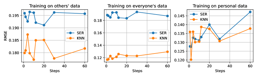
(a) Input from all signals

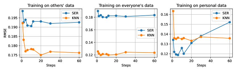
(b) Input from sac/acc3d signals

Figure 4: RMSE of GRF predicted with SER and KNN for different numbers of steps $S$ in a batch

4.2 $k$-Nearest Neighbors Regression

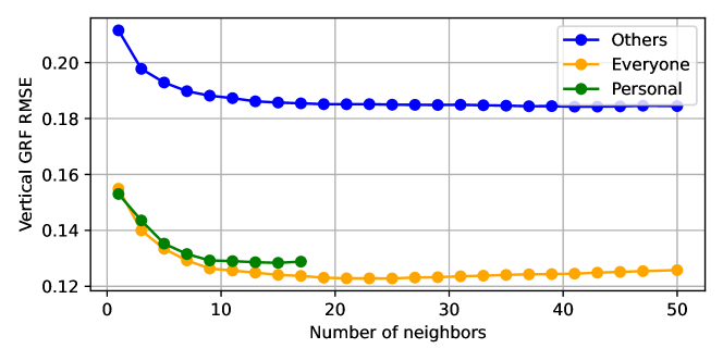
Figure 5: RMSE of vertical GRF for different numbers of neighbors $k$ using KNN regression

As a lightweight baseline, we apply $k$-Nearest Neighbors regression (KNN), where the GRF is predicted by combining the GRF signals of the $k$ training examples with most similar IMU signals. Specifically, given the IMU signals $x\in\mathbb{R}^{1\times m}$ for a new sequence of $S$ steps, we predict its GRF signals $y\in\mathbb{R}^{1\times p}$ by:

1. Sorting the sequences of $S$ steps of the training set, $x_{i}\in\mathbb{R}^{1\times m}$ for $i=1,\dots,n$, by their Euclidean distances $d(x,x_{i})=\lVert x-x_{i}\rVert_{2}$;

2. Selecting the indices $\mathcal{K}\subseteq\{1,\dots,n\}$ of the $k$ training sequences with lowest distances;

3. Predicting $y\in\mathbb{R}^{1\times p}$ as

   $$y=\frac{\sum_{i\in\mathcal{K}}d(x,x_{i})\,y_{i}}{\sum_{i\in\mathcal{K}}d(x,x_{i})}$$

   where $y_{i}\in\mathbb{R}^{1\times p}$ are the GRF signals associated with the IMU signals $x_{i}$ in the training set, for $i=1,\dots,n$.

For each prediction task, we select the number of neighbors $k$ and the number of consecutive steps $S$ in a sequence using a validation set. While $k$ has a minor effect on prediction accuracy (additional neighbors after $k=10$ have lower weights and provide minor improvements, as illustrated in Fig. 5), $S$ can have an important effect for some prediction tasks, as illustrated in Fig. 4.

4.3 Long Short-term Memory Networks

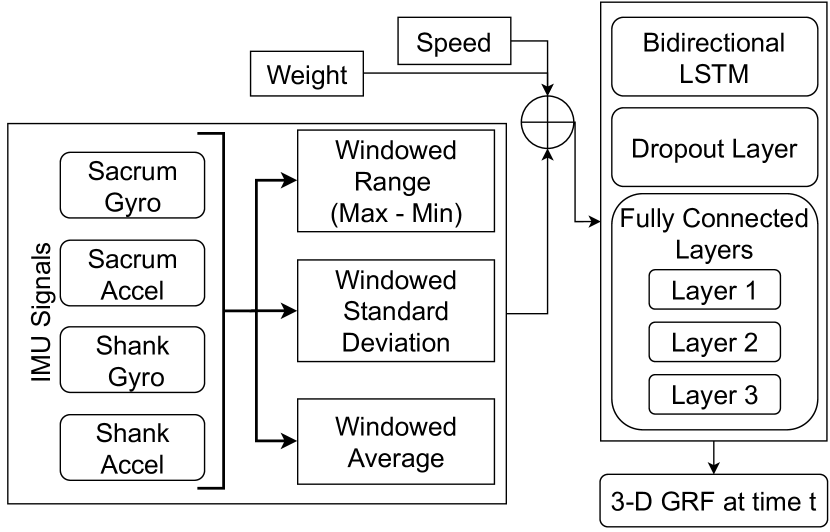
Figure 6: LSTM Architecture

Hyperparameter	Values
LSTM Units	125, 250, 300, 500, 800, 1000
Layer 1 Neurons	5, 10, 20, 35, 50
Layer 2 Neurons	10, 20, 35, 50
Layer 3 Neurons	5, 10, 20, 35, 50
Batch Size	8, 16, 32
Learning Rate	0.0001, 0.0003, 0.0005, 0.0007, 0.001
Dropout Rate	0.2, 0.4

Table 1: LSTM Hyperparameter Search Space

As a deep learning baseline, we adapt the state-of-the-art long short-term memory (LSTM) neural network of [14] to predict all components of the GRF (instead of the only vertical component predicted in [14]). The model predicts $\vec{g}(t)=\big{(}g_{x}(t),g_{y}(t),g_{z}(t)\big{)}$ from the IMU signals in the time window $[t-W,t]$ of size $W>0$ (e.g., in the all case, $\lVert\vec{a}_{s}(u)\rVert,\lVert\vec{a}_{lr}(u)\rVert,\lVert\vec{\omega}_{s}(u)\rVert,\lVert\vec{\omega}_{lr}(u)\rVert$ for $u\in[t-W,t]$). Similarly to [14], we also provide the mean, standard deviation and range of IMU signals over the window $[t-W,t]$ as inputs, together with the running speed and the weight of the athlete.

The architecture of the network is depicted in Fig. 6: after a bidirectional LSTM layer with tanh activations and dropout (a regularization approach), we use three fully-connected layers with ReLU activations. The model is trained using the Adam optimizer as a standard choice and the mean square error as loss function. We select the number of units of each layer, batch size, learning rate, and dropout rate using a validation set; the search space is reported in Table 1. Notably, this machine learning approach has much higher training times than ser and knn (up to 1 hour for each combination of hyperparameters) and the largest search space (18,000 combinations of hyperparameters). Due to memory limitations of the GPUs used for training (NVIDIA Titan X, 12 GB of RAM [22]), we were not able to train models with more than 1000 LSTM units, although hyperparameter selection suggests that a higher number of LSTM units could be beneficial, although quite costly.

5 Results and Discussion

	Scenario others				Scenario everyone				Scenario personal
Input Signals	ser	knn	lstm		ser	knn	lstm		ser	knn	lstm
all	0.197	0.180	0.126		0.187	0.118	0.124		0.130	0.122	0.134
acc	0.220	0.197	0.177		0.210	0.125	0.175		0.127	0.127	0.143
ang	0.197	0.187	0.183		0.190	0.130	0.183		0.133	0.132	0.171
shank	0.215	0.210	0.206		0.205	0.149	0.209		0.139	0.134	0.188
sacrum	0.217	0.210	0.289		0.205	0.129	0.286		0.136	0.137	0.184
sac/acc3d	0.194	0.181	0.171		0.185	0.122	0.177		0.128	0.132	0.178
sac/acc	0.198	0.190	0.187		0.190	0.130	0.206		0.129	0.133	0.193

Table 2: RMSE (in body weight units, BW) of vertical GRF predictions $RMSE(g_{z},\hat{g}_{z})$ for different input signals, scenarios, machine learning methods (results highlighted in blue are optimal or less than 0.010 from optimal for a scenario and set of input signals)

	Scenario others			Scenario everyone			Scenario personal
Input Signals	ser	knn	lstm	ser	knn	lstm	ser	knn	lstm
all	$6.5$	$6.0$	$4.2$	$6.2$	$3.9$	$4.2$	$4.2$	$4.0$	$4.3$
acc	$7.4$	$6.6$	$6.0$	$7.0$	$4.1$	$5.9$	$4.1$	$4.1$	$4.8$
ang	$6.5$	$6.2$	$6.1$	$6.3$	$4.3$	$6.0$	$4.3$	$4.3$	$5.9$
shank	$7.2$	$7.0$	$7.0$	$6.8$	$4.9$	$7.0$	$4.5$	$4.4$	$6.5$
sacrum	$7.2$	$6.9$	$10.1$	$6.8$	$4.2$	$9.8$	$4.4$	$4.5$	$6.3$
sac/acc3d	$6.4$	$6.0$	$5.8$	$6.2$	$4.0$	$5.9$	$4.1$	$4.3$	$6.0$
sac/acc	$6.6$	$6.3$	$6.3$	$6.3$	$4.3$	$6.9$	$4.2$	$4.4$	$6.5$

Table 3: rRMSE (%) of vertical GRF predictions $rRMSE(g_{z},\hat{g}_{z})$ for different input signals, scenarios, machine learning methods (results highlighted in blue are optimal or less than 0.5% from optimal for a scenario and set of input signals)

	Scenario others				Scenario everyone				Scenario personal
Input Signals	ser	knn	lstm		ser	knn	lstm		ser	knn	lstm
all	0.001	2.256	0.497		0.001	2.088	0.472		0.001	0.042	0.558
acc	0.003	1.165	0.521		0.002	1.089	0.473		0.001	0.022	0.586
ang	0.004	1.161	0.543		0.0004	1.064	0.474		0.001	0.025	0.516
shank	0.005	1.165	0.503		0.002	1.062	0.476		0.001	0.021	0.554
sacrum	0.004	1.156	0.545		0.0004	1.067	0.480		0.001	0.023	0.563
sac/acc3d	0.001	1.716	0.439		0.002	1.574	0.579		0.001	0.030	0.248
sac/acc	0.005	0.518	0.450		0.002	0.411	0.461		0.001	0.013	0.272

Table 4: Average inference time in seconds predicting 3D GRF of a collection (120-180 steps) for an athlete.

Acronym	Input Signals	Description
all	$\lVert\vec{a}_{s}(t)\rVert,\lVert\vec{a}_{lr}(t)\rVert,\lVert\vec{\omega}_{s}(t)\rVert,\lVert\vec{\omega}_{lr}(t)\rVert$	L2 norm of all acceleration and angular velocity signals
acc	$\lVert\vec{a}_{s}(t)\rVert,\lVert\vec{a}_{lr}(t)\rVert$	L2 norm of acceleration signals (sacrum, left/right shanks)
ang	$\lVert\vec{\omega}_{s}(t)\rVert,\lVert\vec{\omega}_{lr}(t)\rVert$	L2 norm of angular velocity signals (sacrum, left/right shanks)
sacrum	$\lVert\vec{a}_{s}(t)\rVert,\lVert\vec{\omega}_{s}(t)\rVert$	L2 norm of acceleration and angular velocity at the sacrum
shanks	$\lVert\vec{a}_{lr}(t)\rVert,\lVert\vec{\omega}_{lr}(t)\rVert$	L2 norm of acceleration and angular velocity at left/right shanks
sac/acc3d	$\vec{a}_{s}(t)$	$x,y,z$ components of acceleration signal at the sacrum
sac/acc	$\lVert\vec{a}_{s}(t)\rVert$	L2 norm of acceleration signal at the sacrum

Table 5: Combinations of input signals for the prediction tasks

Acronym	Training Data of the Scenario
others	IMU and GRF data of other athletes
personal	IMU and GRF data of the same athlete
everyone	IMU and GRF data of all athletes

Table 6: Scenarios for the prediction tasks

5.1 Prediction of the Normal GRF Waveform

First, we focus on $RMSE(g_{z},\hat{g}_{z})$ and $rRMSE(g_{z},\hat{g}_{z})$ (i.e., RMSE and rRMSE of the vertical GRF) predictions by different machine learning methods for each set of input signals and scenario, because the vertical component of the GRF is associated with the prediction of stress responses in bone and soft tissue which has been a focus of running-related injury research [2, 3] and provides the information used to compute several discrete biomechanical variables. Results are reported in Tables 2 and 3, while input signals and scenarios of different prediction tasks are summarized in Tables 5 and 6, respectively. Although limited to our dataset, this evaluation allows us to make the following observations regarding the use of machine learning methods for the prediction of GRF from IMU signals.

5.1.1 Use of Acceleration and Angular Velocity Signals

We observe that, in all scenarios and for all machine learning methods, the use of both acceleration and angular velocity signals is preferable, since RMSE and rRMSE are similar or significantly lower. In particular, using only acceleration (case acc) or angular velocity signals (case ang) is generally worse than using both (case all). Since most IMU sensors collect both signals, these improvements can be obtained without additional costs of the data collection process, despite the focus of related work on the exclusive use of acceleration signals [14].

5.1.2 Sensor Locations

We observe that, in all scenarios and for all machine learning methods, the use of sensors at both sacrum and left/right shank (case all) is preferable, since RMSE and rRMSE are either similar or significantly lower than when each sensor location is used exclusively (cases sacrum and shank, respectively). While expected for deep learning methods (lstm), this result highlights that lightweight machine learning methods such as ser and knn can also provide effective prediction models for complex IMU data collected from multiple locations.

5.1.3 Use of Multidimensional Acceleration at the Sacrum

Since related literature [16, 14] focuses on acceleration signals collected using sensors located at the sacrum, we explore the benefits of a multidimensional acceleration signal $\vec{a}_{s}(t)$ (sac/acc3d) to predict GRF, instead of its L2 norm $\lVert\vec{a}_{s}(t)\rVert$ (case sac/acc). We observe that, in all scenarios and for all machine learning methods, the use of a multidimensional acceleration signal at the sacrum is preferable to its L2 norm, since RMSE and rRMSE are either similar or significantly lower. We also note that, when limited to the sacrum location, the use of multidimensional acceleration signals (sac/acc3d) is preferable to the use of the L2 norm of both acceleration and angular velocity (sacrum), and even to the use of the L2 norm of only acceleration signals at the sacrum and left/right shanks (acc). Our experiments indicate that the increase in the model computation cost is negligible.

5.1.4 Use of Lightweight Machine Learning Methods

While state-of-the-art approaches [14] adopt deep learning methods based on lstm neural networks, we observe that lightweight approaches can provide similar or better accuracy of the predicted GRF for specific scenarios and input signals. In the scenario everyone, knn is preferable to lstm and ser, as it provides much lower RMSE and rRMSE for most combinations of input signals; in the scenario personal, both ser and knn are preferable to lstm, for all combinations of input signals. Notably, in the setting of [14] (scenario others, signals sac/acc3d), knn and lstm perform very similarly on our dataset (RMSE of 0.181 and 0.171, respectively; as a reference, lstm incurred an RMSE of $0.16$ in [14]).

We attribute the improved performance of knn in the scenarios everyone and personal to the inclusion of historical running data collected for the target athlete in the training set: knn is able to exploit the patterns specific to the target athlete, while ignoring data from other athletes; in contrasting with lstm (similar accuracy between others and everyone scenarios), which improves prediction accuracy from having more sensor data as input from multiple body locations. Finally, ser is able to model the GRF of an athlete very accurately in the personal scenario.

Consider inference latency, ser has the shortest inference time in all scenarios (Table 4) using CPUs. The inference time of lstm (using GPU) is dependent on the size of the model such as the number of parameters, layers, and etc, which are determined by a hyper-parameter search whereas knn’s inference time is based on the size of training data.

5.2 Artifacts in Predicted Waveforms

We observe that each machine learning method can result in different anomalies in the predicted GRF, which are significant for its evaluation by domain experts.

For example, the predictions in Fig. 7(a) are for a heel-strike runner with a very pronounced impact peak associated with the runner initiating ground contact with their heel. In the scenario others, only lstm predicts a pronounced impact peak, while knn and ser predict smoother waveforms due to the averaging of data from mid-foot and front-foot runners (initiating ground contact with their mid or forefoot) with less pronounced impact peak. Both lstm and knn are able to use data of heel-strike runners in the scenarios everyone and personal, while ser accurately predicts this feature only in the scenario personal.

In Fig. 7(b), we report the GRF of a front-foot striker with no visible impact peak. In the scenarios others and everyone, knn and ser introduce an initial peak not present in the measured GRF; in contrast, lstm introduces a minor peak in the scenario personal. When athletes have a minor impact peak as in Fig. 7(c), knn and ser tend to produce more representative waveforms, in all scenarios.

Finally, the athlete of Fig. 7(d) also has a pronounced impact peak. While knn and ser predict a smoother waveform resulting from the average of these patterns, lstm tries to capture both the initial front of the GRF due to the impact peak and also its active peak, resulting in inaccurate waveforms in the others and everyone scenarios. The same phenomenon is observed when using only acceleration signals at the sacrum (Fig. 7(e)); when using multidimensional acceleration signals (acc3d), similar anomalies are produced by ser (cases others and everyone).

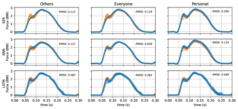
(a) Athlete 1 (Major Impact Peak), Signals all

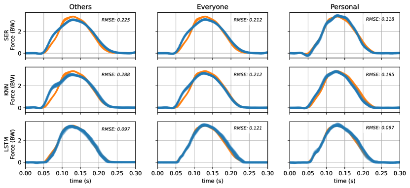
(b) Athlete 2 (No Impact Peak), Signals all

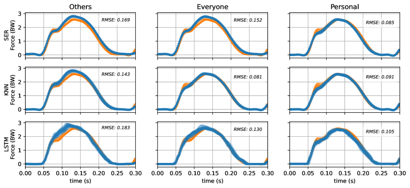
(c) Athlete 3 (Minor Impact Peak), Signals all

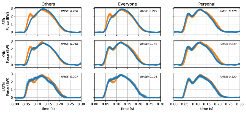
(d) Athlete 4 (Major Impact Peak), Signals all

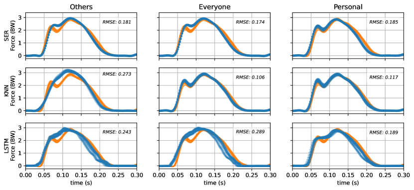
(e) Athlete 4 (Major Impact Peak), Signals sac/acc

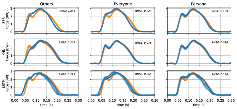
(f) Athlete 4 (Major Impact Peak), Signals acc3d

Figure 7: Comparing predictions (blue) and measurements (orange) of normal GRF $g_{z}(t)$ of selected athletes for different scenarios, input signals, machine learning methods

5.3 Prediction of Discrete Biomechanical Variables

	Scenario others			Scenario everyone			Scenario personal
Biomechanical Variable	ser	knn	lstm	ser	knn	lstm	ser	knn	lstm
Loading Rate	$19.4$	$19.6$	$11.6$	$19.4$	$6.5$	$13.6$	$7.2$	$4.9$	$10.0$
Contact Time	$9.9$	$10.9$	$8.8$	$12.1$	$4.7$	$6.4$	$4.3$	$4.1$	$4.7$
Braking Time	$3.9$	$3.5$	$5.9$	$5.9$	$2.0$	$4.3$	$3.1$	$1.7$	$4.5$
Braking Percentage	$9.5$	$7.4$	$8.6$	$9.2$	$3.9$	$5.1$	$4.6$	$4.3$	$5.2$
Active Peak	$5.6$	$4.7$	$1.6$	$5.3$	$2.8$	$1.3$	$2.9$	$2.6$	$2.6$
Average Vert. Force	$5.9$	$4.9$	$3.2$	$6.2$	$2.5$	$3.1$	$2.4$	$2.2$	$2.8$
Net Vertical Impulse	$10.5$	$8.3$	$5.6$	$10.6$	$4.3$	$5.6$	$4.1$	$4.3$	$8.4$
A/P Velocity Change	$12.8$	$11.1$	$11.4$	$10.0$	$5.4$	$9.3$	$7.3$	$6.4$	$8.7$

Table 7: MAPE (%) of discrete biomechanical variables predicted from all input signals for different scenarios and machine learning methods (results highlighted in blue are optimal or less than 0.5% from optimal for a scenario and biomechanical variable)

Finally, we use the predicted GRF waveform to evaluate discrete biomechanical variables (defined precisely in Appendix A), which are of interest to domain experts for the detection of running anomalies that may lead to stress-responses in bone and soft tissue. MAPE values with respect to the measured GRF are reported in Table 7 for GRF predictions using all input signals, for different scenarios and machine learning methods.

In the scenario others, lstm achieves substantially lower MAPE for most biomechanical variables (except breaking time and braking percentage), in line with the lower RMSE and rRMSE values of the predicted GRF waveform (Tables 2 and 3, row all). In contrast, in the scenario everyone, lstm achieves substantially higher MAPE than knn, despite their similar RMSE and rRMSE values in Tables 2 and 3.

In the scenario personal, knn and ser achieve substantially lower MAPE than lstm for several biomechanical variables, e.g., loading rate and net vertical impulse, as expected. Notably, while the best RMSE and rRMSE achieved by knn in the scenario personal (Tables 2 and 3, row all) are worse than those of the scenario everyone, its MAPE values are substantially lower for most biomechanical variables; unexpected MAPE reductions are observed in the scenario personal also for lstm (e.g., for loading rate and contact time). In general, similarly to related work [14], MAPE values are significantly higher for biomechanical variables that depend on sensitive features of the GRF waveform, e.g., the loading rate, which depends on rate of change of the vertical GRF.

This analysis shows that RMSE and rRMSE of the predicted GRF are not always useful estimates of the accuracy of the derived biomechanical variables (which depend on specific features of the GRF waveform), and that personal data is especially useful when biomechanical variables are of interest. The presence of various types of artifacts in the predictions from others’ data, despite achieving a low RMSE, highlights the potential for further improvements.

6 Related Work

The prediction of GRF from IMU sensor data is addressed in several works such as [23, 17, 16] to overcome the difficulty of direct GRF measurement, while the use of GRF and discrete biomechanical variables to predict stress-responses in bone and soft tissue is addressed in [7, 24, 25].

Similarly to the SER method proposed in this paper, the approach of [26] uses the general idea of transduction [19] between the embeddings of input IMU data and output GRF data. We observe the following critical differences between ser and [26]:

• ser uses a different organization of the training data, where the running steps and their IMU and GRF signals are split into batches; as shown in Fig. 4 where the best batch size is generally more than 1. Batch size is a critical hyperparameter to consider intra-step interactions (optimized with a validation set) as opposed to using a single step without differentiating left and right foot (as in [26]) which results in lower accuracy. (ser separates left and right side when batch size is 1). This also suggests that the control of one leg may be different than that of the other.

• ser uses SVD instead PCA (used in [26]), i.e., it does not normalize each input variable of IMU or GRF timeseries across the entire dataset. This difference allows us to preserve the patterns of the step signals over time (e.g., the impact peaks followed by the active GRF peak).

• ser uses least squares regression to predict the output embedding instead of neural networks (used in [26]); in our experiments, neural networks (with up to 5 layers and 100 neurons per layer) resulted in lower accuracy and slower training, due to the limited available data and additional hyperparameter optimization.

Notably, while the approach of [26] performs worse than state-of-the-art methods using LSTM neural networks [14, 27], ser performs similarly or better in the personal scenario, with much lower training times (as discussed in Section 5).

While the works [14] and [27] focus on the prediction of the vertical component for the GRF from IMU sensor signals, [28] predicts both vertical and anterior–posterior components from plantar pressure, also using bidirectional LSTM models; field-specific knowledge such as lower body kinematics is combined in the prediction models in [29, 30], while the use of a high number of IMU sensors is explored in [31].

7 Conclusions

GRF waveforms and their derived biomechanical variables can be accurately predicted from acceleration and angular velocity signals collected using wearable IMU sensors. To this end, depending on the training data and input signals, simple machine learning methods such as SER and KNN are similarly accurate or more accurate than LSTM neural networks, using fewer computation resources or energy and with much faster training times and hyperparameter optimization, as illustrated by our evaluation.

Notably, SER and KNN produce more accurate predictions of the GRF waveform when personal training data (i.e., GRF and IMU measurements for an athlete) are available; in this case, the accuracy of the predicted biomechanical variables is greatly improved with respect to LSTM neural networks. We also observed that all machine learning methods benefit from the use of both acceleration and angular velocity, and from the use of all components of the sacrum acceleration (instead of its L2 norm).

In future work, we plan to evaluate the use of predicted GRF waveforms and biomechanical variables for the detection of running anomalies leading to injuries.

Appendix A Discrete Biomechanical Variables

We consider the following discrete biomechanical variables (or gait metrics) from [1, 14] to evaluate our GRF predictions. Let $g_{x},g_{y}$ and $g_{z}$ be the components of the GRF of a step (after a 50 Hz low-pass filter and normalized by body weight, with unit denoted as $BW$); the start time $T_{s}$ (in seconds) is the time when the vertical GRF reaches 50 N, i.e., $T_{s}=\min\{\,t\mid BW\cdot g_{z}(t)>50\,\}$, while the end time $T_{e}$ is the time when the vertical GRF drops below 50 N, i.e., $T_{e}=\min\{\,t>T_{s}\mid BW\cdot g_{z}(t)<50\,\}$.

• Loading Rate ($BW\cdot s^{-1}$): Average slope of the vertical GRF during the first 25 ms of the stance after reaching the 50 N threshold [32], i.e.,

  $$\text{Loading Rate}=\frac{g_{z}(T_{s}+0.025)-g_{z}(T_{s})}{0.025}\,.$$

• Contact Time ($s$): Time during which the vertical GRF is above 50 N, i.e., $T_{c}=T_{e}-T_{s}$.

• Braking Time ($s$): Time during which the vertical GRF signal is above the threshold and the A/P GRF component is negative, i.e.,

  $$T_{b}=|\{T_{s}\leq t\leq T_{e}\mid g_{y}(t)<0\}|\,.$$

• Braking Percentage: Percentage of contact time spent in braking, i.e., $T_{b}/T_{c}$.

• Active Peak ($BW$): Maximum vertical GRF between 30-100% of the stance (to exclude the impact peak), i.e., $\max\{\,g_{z}(t)\,|\,t>T_{s}+0.3T_{c}\,\}$.

• Average Vertical Force $(BW)$: Average value of the vertical GRF, i.e., $\frac{1}{T_{c}}\int_{T_{s}}^{T_{e}}g_{z}(t)\,dt$.

• Net Vertical Impulse ($BW\cdot s$): Area under the vertical GRF reduced by the body weight unit, i.e., $\big{(}\int_{T_{s}}^{T_{e}}g_{z}(t)\,dt\big{)}-1$.

• A/P Velocity Change $(m\cdot s^{-1})$: Change in velocity along the A/P force direction, i.e., $9.81\cdot(\textit{A/P Impulse})$, where the A/P Impulse ($BW\cdot s$) is the area between the A/P GRF component and the zero line, i.e., $\int_{T_{s}}^{T_{e}}g_{y}(t)\,dt$.

Appendix B Aligning Signals from Different Locations by Reference Events

To predict GRF from IMUs, timestamps and gait events need to match consistently across different signals and locations. For a model that predicts the entire stance in GRF from signals of an entire stance in IMU signals, training the model would require supplying signals aligned by their corresponding steps. Similarly for models predicting one sample point at a time based on samples of other signals at the same time point, signals at different locations need to synchronize. Given acceleration and angular velocity measurements of a IMU sensor are synchronized, we manually aligned data from IMU sensors at different locations and GRF data from the treadmills (which was downsampled to 500 Hz to match the IMU frequency and normalized by the body weight of the athlete).

In our dataset, IMU sensors at different locations (sacrum and shanks) and GRF measured from force plates are sampled by individual clocks. Although we do not observe any servery non-linear drifts, linear drifts and time delays are significantly affecting the alignment of gait events.

To align all gait events over a series of continuous running steps, the dataset includes reference events where the athlete jumps in-place before and after continuously running on an instrumented treadmill. Wearing all sensors, the athlete jumping in-place creates a unique signal pattern across all sensors with a sharp edge marking the time instance when both feet striking the ground after flight. An example of aligned signals at the jump reference is shown in Fig. 8(a). We align both reference events before and after a run by shifting and linearly stretching the signals to correct time delays and linear drifts. We use GRF as the referencing signal and edit IMU signals to align with GRF. After aligning both reference events, signals for each running steps between the references are also aligned.

After aligning data from different sensors, each running measurement is automatically split into steps by identifying the maxima of the correlation between the L2 norm of shank acceleration and a reference signal (a triangular signal with 100 ms duration followed by a zero signal of 100 ms, mimicking the patterns observed in acceleration signals). Steps of a running measurement are aligned by maximizing their pairwise correlation; then, a fixed delay is applied to all the steps in a measurement to maximize their mean correlation with the reference signal, in order to align them with steps of other measurements (i.e., at different running speeds or for different athletes). We manually check the alignment of signals for each foot contact by overlapping all steps from each run (an example of such view is shown in Fig. 8(b).). Aligning these signals by the start and end points shows time drifts between signals are only linear and the overlapped view shows gait events within each steps are aligned similarly. While there is no guarantee for each sample point across all signal types is aligned perfectly, models looking at an entire stance or a windowed signals greater or equal to a stance should have a consistent amount of information.

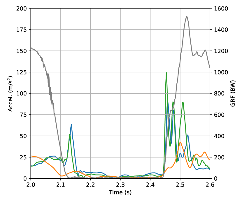
(a)

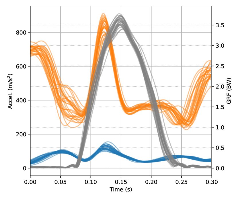
(b)

Figure 8: Examples of overlapping GRF with acceleration signals from shanks and sacrum. Blue is from left shank, green is from right shank, orange is from sacrum, and grey is GRF. 8(a)) Aligned jump reference. 8(b)) Consecutive left steps under a constant speed.

References

- [1] C. F. Munro, D. I. Miller, A. J. Fuglevand, Ground reaction forces in running: a reexamination, Journal of Biomechanics 20 (2) (1987) 147–155.
- [2] P. R. Cavanagh, M. A. Lafortune, Ground reaction forces in distance running, Journal of Biomechanics 13 (5) (1980) 397–406.
- [3] S. L. James, B. T. Bates, L. R. Osternig, Injuries to runners, The American Journal of Sports Medicine 6 (2) (1978) 40–50.
- [4] A. Hreljac, Impact and overuse injuries in runners, Medicine and Science in Sports and Exercise 36 (5) (2004) 845–849.
- [5] J. Bigouette, J. Simon, K. Liu, C. L. Docherty, Altered vertical ground reaction forces in participants with chronic ankle instability while running, Journal of Athletic Training 51 (9) (2016) 682–687.
- [6] D. Kiernan, D. A. Hawkins, M. A. Manoukian, M. McKallip, L. Oelsner, C. F. Caskey, C. L. Coolbaugh, Accelerometer-based prediction of running injury in national collegiate athletic association track athletes, Journal of Biomechanics 73 (2018) 201–209.
- [7] C. Napier, C. MacLean, J. Maurer, J. Taunton, M. Hunt, Kinetic risk factors of running-related injuries in female recreational runners, Scandinavian Journal of Medicine & Science in Sports 28 (10) (2018) 2164–2172.
- [8] S. P. Messier, D. F. Martin, S. L. Mihalko, E. Ip, P. DeVita, D. W. Cannon, M. Love, D. Beringer, S. Saldana, R. E. Fellin, et al., A 2-year prospective cohort study of overuse running injuries: the runners and injury longitudinal study (trails), The American Journal of Sports Medicine 46 (9) (2018) 2211–2221.
- [9] P. O. Riley, J. Dicharry, J. Franz, U. Della Croce, R. P. Wilder, D. C. Kerrigan, A kinematics and kinetic comparison of overground and treadmill running, Medicine & Science in Sports & Exercise 40 (6) (2008) 1093–1100.
- [10] B. Kluitenberg, S. W. Bredeweg, S. Zijlstra, W. Zijlstra, I. Buist, Comparison of vertical ground reaction forces during overground and treadmill running. a validation study, BMC Musculoskeletal Disorders 13 (1) (2012) 1–8.
- [11] M. J. Asmussen, C. Kaltenbach, K. Hashlamoun, H. Shen, S. Federico, B. M. Nigg, Force measurements during running on different instrumented treadmills, Journal of Biomechanics 84 (2019) 263–268.
- [12] D. A. Jacobs, D. P. Ferris, Estimation of ground reaction forces and ankle moment with multiple, low-cost sensors, Journal of Neuroengineering and Rehabilitation 12 (1) (2015) 1–12.
- [13] E. Dorschky, M. Nitschke, C. F. Martindale, A. J. van den Bogert, A. D. Koelewijn, B. M. Eskofier, CNN-Based Estimation of Sagittal Plane Walking and Running Biomechanics From Measured and Simulated Inertial Sensor Data, Frontiers in Bioengineering and Biotechnology 8 (2020). doi:10.3389/fbioe.2020.00604.
- [14] R. S. Alcantara, W. B. Edwards, G. Y. Millet, A. M. Grabowski, Predicting continuous ground reaction forces from accelerometers during uphill and downhill running: a recurrent neural network solution, PeerJ 10 (2022) e12752. doi:10.7717/peerj.12752.
- [15] H. E. Stewart, R. S. Alcantara, K. A. Farina, Can ground reaction force variables pre-identify the probability of a musculoskeletal injury in collegiate distance runners, under review (2023).
- [16] R. S. Alcantara, E. M. Day, M. E. Hahn, A. M. Grabowski, Sacral acceleration can predict whole-body kinetics and stride kinematics across running speeds, PeerJ 9 (2021) e11199. doi:10.7717/peerj.11199.
-
[17]
W. R. Johnson, A. Mian, M. A. Robinson, J. Verheul, D. G. Lloyd, J. A.
Alderson, Multidimensional
ground reaction forces and moments from wearable sensor accelerations via
deep learning, IEEE Trans. Biomed. Eng. 68 (1) (2021) 289–297.
doi:10.1109/TBME.2020.3006158.
URL https://doi.org/10.1109/TBME.2020.3006158 - [18] E. Bair, T. Hastie, D. Paul, R. Tibshirani, Prediction by supervised principal components, Journal of the American Statistical Association 101 (473) (2006) 119–137.
- [19] C. Cortes, M. Mohri, J. Weston, A general regression technique for learning transductions, in: ICML 2005, Vol. 119 of ACM International Conference Proceeding Series, ACM, 2005, pp. 153–160. doi:10.1145/1102351.1102371.
- [20] S. Venturi, T. Casey, Svd perspectives for augmenting deeponet flexibility and interpretability, Computer Methods in Applied Mechanics and Engineering 403 (2023) 115718.
- [21] Q. Liao, Q. Zhang, Efficient rank-one residue approximation method for graph regularized non-negative matrix factorization, in: Machine Learning and Knowledge Discovery in Databases: European Conference, ECML PKDD 2013, Prague, Czech Republic, September 23-27, 2013, Proceedings, Part II 13, Springer, 2013, pp. 242–255.
-
[22]
NVIDIA,
NVIDIA
TITAN X Graphics Card (2023).
URL https://www.nvidia.com/en-us/geforce/products/10series/titan-x-pascal/ - [23] G. Leporace, L. A. Batista, J. Nadal, Prediction of 3d ground reaction forces during gait based on accelerometer data, Research on Biomedical Engineering 34 (2018) 211–216.
- [24] C. D. Johnson, A. S. Tenforde, J. Outerleys, J. Reilly, I. S. Davis, Impact-related ground reaction forces are more strongly associated with some running injuries than others, The American Journal of Sports Medicine 48 (12) (2020) 3072–3080.
- [25] C. N. Vannatta, B. L. Heinert, T. W. Kernozek, Biomechanical risk factors for running-related injury differ by sample population: A systematic review and meta-analysis, Clinical Biomechanics 75 (2020) 104991.
- [26] M. Pogson, J. Verheul, M. A. Robinson, J. Vanrenterghem, P. Lisboa, A neural network method to predict task-and step-specific ground reaction force magnitudes from trunk accelerations during running activities, Medical Engineering & Physics 78 (2020) 82–89.
- [27] S. R. Donahue, M. E. Hahn, Estimation of gait events and kinetic waveforms with wearable sensors and machine learning when running in an unconstrained environment, Scientific Reports 13 (1) (2023) 2339.
- [28] E. C. Honert, F. Hoitz, S. Blades, S. R. Nigg, B. M. Nigg, Estimating running ground reaction forces from plantar pressure during graded running, Sensors 22 (9) (2022) 3338.
- [29] D.-S. Komaris, E. Pérez-Valero, L. Jordan, J. Barton, L. Hennessy, B. O’Flynn, S. Tedesco, Predicting three-dimensional ground reaction forces in running by using artificial neural networks and lower body kinematics, IEEE Access 7 (2019) 156779–156786.
- [30] B. L. Scheltinga, J. N. Kok, J. H. Buurke, J. Reenalda, Estimating 3d ground reaction forces in running using three inertial measurement units, Frontiers in Sports and Active Living 5 (2023) 1176466.
- [31] F. J. Wouda, M. Giuberti, G. Bellusci, E. Maartens, J. Reenalda, B.-J. F. Van Beijnum, P. H. Veltink, Estimation of vertical ground reaction forces and sagittal knee kinematics during running using three inertial sensors, Frontiers in Physiology 9 (2018) 218.
- [32] J. R. Yong, A. Silder, K. L. Montgomery, M. Fredericson, S. L. Delp, Acute changes in foot strike pattern and cadence affect running parameters associated with tibial stress fractures, Journal of biomechanics 76 (2018) 1–7.