$\text{L}^{2}$ solutions for cubic NLS equation with fractional elliptic/hyperbolic operators on ${\mathbb{R}}\times{\mathbb{T}}$ and ${\mathbb{R}}^{2}$

Abstract.

In this work we consider the Cauchy problem for the cubic Schrödinger equation posed on cylinder ${\mathbb{R}}\times{\mathbb{T}}$ with fractional derivatives $(-\partial_{y}^{2})^{\alpha},\,\alpha>0$, in the periodic direction. The spatial operator includes elliptic and hyperbolic regimes. We prove $L^{2}$ global well-posedness results when $\alpha>1$ by proving a $L^{4}-L^{2}$ Strichartz inequality for the linear equation, following the ideas in [15], where it was considered the elliptical case with $\alpha=1$. Further, these results remain valid on the euclidean environment ${\mathbb{R}}\times{\mathbb{R}}$, so well-posedness in $L^{2}$ are also achieved in this case. Our proof in the elliptic (hyperbolic) case does not work in the case $0<\alpha<1$ ($0<\alpha\leq 1$), respectively.

1. Introduction

We consider the Cauchy problem associated to the cubic nonlinear Schrödinger equation (NLS) on cylinder with fractional derivatives in the periodic direction. More precisely, we will study the initial value problem (IVP):

$$\begin{cases}i\partial_{t}u+{\mathcal{L}}^{\pm}_{\alpha}u=\nu|u|^{2}u,&(x,y)\in{\mathbb{R}}\times{\mathbb{T}},~{}~{}t\in{\mathbb{R}},\vskip 6.0pt plus 2.0pt minus 2.0pt\\ u(0;x,y)=\phi(x,y),&(x,y)\in{\mathbb{R}}\times{\mathbb{T}},\end{cases}$$ (1.1)

where $\nu\in{\mathbb{R}}$, $u$ is a complex-valued function on ${\mathbb{R}}\times{\mathbb{T}}\times{\mathbb{R}}$, with ${\mathbb{T}}={\mathbb{R}}/2\pi{\mathbb{Z}}$, and ${\mathcal{L}}^{\pm}_{\alpha}$ denotes the pseudo-differential operator

$${\mathcal{L}}^{\pm}_{\alpha}:=\partial^{2}_{x}\mp(-\partial^{2}_{y})^{\alpha},\quad\text{with}\;\alpha>0,$$ (1.2)

defined in Fourier variables by

$$\widehat{{\mathcal{L}}^{\pm}_{\alpha}f}(\xi,n)=-(\xi^{2}\pm|n|^{2\alpha})\widehat{f}(\xi,n),$$ (1.3)

with Fourier transform

$${\mathcal{F}}f(\xi,n)=\widehat{f}(\xi,n):=\frac{1}{2\pi}\int_{-\infty}^{\infty}\int_{0}^{2\pi}f(x,y)e^{-i(x\xi+ny)}dydx.$$ (1.4)

The cases $\nu<0$ and $\nu>0$ are known as the focusing and defocusing regimes, respectively.

Note that in the case $\alpha=1$,

$${\mathcal{L}}^{\pm}_{1}=\begin{cases}\partial^{2}_{x}+\partial^{2}_{y}=:\Delta\;\text{(Laplacian operator) in the case (+)},\vskip 6.0pt plus 2.0pt minus 2.0pt\\ \partial^{2}_{x}-\partial^{2}_{y}=:\Box\;\text{(wave operator) in the case (-)}.\end{cases}$$

The linear propagator $U^{\pm}_{\alpha}$ of (1.1) is given by

$$U_{\alpha}^{\pm}(t)\phi=e^{it\,{\mathcal{L}}^{\pm}_{\alpha}}\phi={\mathcal{F}}^{-1}e^{-it(\xi^{2}\pm|n|^{2\alpha})}{\mathcal{F}}\phi.$$ (1.5)

From the physical point of view, the Cauchy problem (1.1) with $\alpha=1$ in the elliptic case appears as a model in several physical problems (see for example the references [10, 12, 17]). On the other hand, in the hyperbolic case it describes, for instance, the gravity waves on liquid surface and ion-cyclotron waves in plasma (see [4, 9, 14]).

In the euclidean domain ${\mathbb{R}}^{2}$, the pseudo-differential operator ${\mathcal{L}}^{\pm}_{\alpha}$, $\alpha>0$, with associated symbol

$$p(\xi,\eta)=\xi^{2}\pm|\eta|^{2\alpha}$$

appears in [5] in the context of existence of analytic solutions.

1.1. Comments about well-posedness in Sobolev spaces for $\boldsymbol{\alpha=1}$

In the euclidean spatial domain ${\mathbb{R}}^{2}$, the existence of local solutions in time for IVP (1.1) with $\alpha=1$ and initial data $\phi\in L^{2}({\mathbb{R}}^{2})$ is a consequence of the time decay estimates coming from dispersion and the Strichartz inequalities, which have the same form for the elliptic or hyperbolic linear Schrödinger equations. For the elliptic operator ${\mathcal{L}}^{+}_{1}$ see [3] and for the hyperbolic case ${\mathcal{L}}^{-}_{1}$ we refer to [6], where the authors deduced Strichartz inequalities for operators $e^{it{\mathcal{L}}}$, where

$${\mathcal{L}}=\sum\limits_{1\leq i,j\leq n}a_{ij}\partial_{x_{i}}\partial_{x_{j}},~{}~{}a_{ij}\in{\mathbb{R}},$$

with non-degenerate quadratic form $A=\big{(}a_{ij}\big{)}$.

In purely periodic domain ${\mathbb{T}}^{2}={\mathbb{T}}\times{\mathbb{T}}$ we refer the reader to [1, 2] for well-posedness in $H^{s}({\mathbb{T}}^{2})$ with $s>0$ in the elliptic case $U^{+}_{1}$, while in the hyperbolic case $U^{-}_{1}$ it was proved in [16] local well-posedness for $s>\frac{1}{2}$ and ill-posedness for $s<\frac{1}{2}$.

On the other hand, on cylinder domain ${\mathbb{R}}\times{\mathbb{T}}$, the elliptical case ${\mathcal{L}}^{+}_{1}$ was treated in [15]. Specifically, the authors showed global well-posedness of IVP (1.1) with $\alpha=1$ for small data in $L^{2}({\mathbb{R}}\times{\mathbb{T}})$. The main tool in the proof is the obtention of the Strichartz inequality for the group $U^{+}_{1}(t)=e^{it\Delta}$ with $(x,y)\in{\mathbb{R}}\times{\mathbb{T}}$, given by

$$\|U_{1}^{+}(t)\phi\|_{L^{4}(I\times{\mathbb{R}}\times{\mathbb{T}})}\leq C_{I}\|\phi\|_{L^{2}({\mathbb{R}}\times{\mathbb{T}})},$$ (1.6)

where $I\subset{\mathbb{R}}$ is an interval containing $t=0$ and $C_{I}$ is a positive constant that depends only on $|I|$ (measure of $I$). Similar Strichartz estimates were obtained in [7] for the energy critical nonlinear Schrödinger equation in partially periodic domains, for instance: ${\mathbb{R}}^{m}\times{\mathbb{T}}^{4-m}$ with $m=2,3$.

In view of the previous comments, a natural question is to figure out what happen for the IVP (1.1) posed on cylinder domains ${\mathbb{R}}\times{\mathbb{T}}$ or ${\mathbb{T}}\times{\mathbb{R}}$.

1.2. Main results

Concerning well-posedness in Sobolev spaces to (1.1) we note that some ill-posedness results for the one-dimensional cubic NLS on the line can be adapted to establish the same results for (1.1) on the cylinder. Indeed, if we consider the following Cauchy problem

$$\begin{cases}i\partial_{t}u+{\mathcal{L}}^{\pm}_{\alpha}u=\nu|u|^{2}u,\qquad&(t;x,y)\in{\mathbb{R}}\times{\mathbb{R}}\times{\mathbb{T}},\vskip 6.0pt plus 2.0pt minus 2.0pt\\ u(0;x,y)=\varphi(x),\end{cases}$$ (1.7)

with $\varphi$ depending only on the $x$-variable and $\varphi\in H^{s}({\mathbb{R}})$, it follows that $\tilde{\varphi}(x,y):=\varphi(x)\in H^{s}({\mathbb{R}}\times{\mathbb{T}})$ with

$$\|\tilde{\varphi}\|_{H^{s}({\mathbb{R}}\times{\mathbb{T}})}=\|\varphi\|_{H^{s}({\mathbb{R}})},$$

and solutions of the IVP:

$$\begin{cases}i\partial_{t}w+\partial^{2}_{x}w=\nu|w|^{2}w,\qquad&x\in\mathbb{R},\;\;t\in{\mathbb{R}},\vskip 6.0pt plus 2.0pt minus 2.0pt\\ w(x,0)=\varphi(x),\end{cases}$$ (1.8)

are also solutions of (1.7). Assuming the existence of local solutions, the IVP (1.8) is ill-posed in the following situations:

1. $s\in(-1/2,0)$ and $\nu<0$. In this case, for any $\delta>0$ the uniform continuous of the flow-map

   $$\Phi:u_{0}\in H^{s}({\mathbb{R}})\longmapsto w\in C([0,\delta];H^{s}({\mathbb{R}}))$$ (1.9)

   fails (see [8]).

2. $s\leq-1/2$ and $\nu\neq 0$. In this case, for any $\delta>0$ the flow-map (1.9) is discontinuous everywhere in $H^{s}({\mathbb{R}})$ (norm inflation arguments, see [11]).

Hence, the statements (i) and (ii) imply similar ill-posedness results for negative Sobolev regularity ($s<0$) to the IVP (1.7) for all $\alpha>0$. In view of these remarks we will consider in this work well-posedness for IVP (1.7) with initial data in $L^{2}({\mathbb{R}}\times{\mathbb{T}})$.

On the other hand, the equation (1.1) posed on ${\mathbb{R}}^{2}$ has the following scaling symmetric property: if $u$ if solution to (1.1), $u_{\lambda}$ is also a solution to (1.1), where

$$u(t;x,y)\longmapsto u_{\lambda}(t;x,y):=\lambda u(\lambda^{2}t;\lambda x,\lambda^{1/\alpha}y),\;\lambda>0.$$ (1.10)

Definition 1.1 (Notion of Criticality).

The scaling (1.10) defines the following notion of criticality in the space $H^{s}({\mathbb{R}}^{2})$.

1. The index $s$ is called critical if   $\|D^{s}u_{\lambda}(0;\cdot,\cdot)\|_{L^{2}({\mathbb{R}}^{2})}\sim\|D^{s}u(0;\cdot,\cdot)\|_{L^{2}({\mathbb{R}}^{2})}$,

2. The index $s$ is called subcritical if   $\|D^{s}u_{\lambda}(0;\cdot,\cdot)\|_{L^{2}({\mathbb{R}}^{2})}\to\infty$ as $\lambda\to\infty$,

3. The index $s$ is called supercritical if   $\|D^{s}u_{\lambda}(0;\cdot,\cdot)\|_{L^{2}({\mathbb{R}}^{2})}\to 0$ as $\lambda\to\infty$.

Computing $\|D^{s}u_{\lambda}(0;\cdot,\cdot)\|_{L^{2}({\mathbb{R}}^{2})}$ for $\lambda>0$ we have

$$\|D^{s}u_{\lambda}(0;\cdot,\cdot)\|^{2}_{L^{2}({\mathbb{R}}^{2})}=\lambda^{1-1/\alpha}\int_{{\mathbb{R}}^{2}}\big{(}\lambda^{2}\xi_{1}^{2}+\lambda^{2/\alpha}\xi_{2}^{2}\big{)}^{s}|\widehat{u}(0;\xi)|^{2}d\xi,$$ (1.11)

with $\xi=(\xi_{1},\xi_{2})$. So one gets

$$\|D^{s}u_{\lambda}(0;\cdot,\cdot)\|^{2}_{L^{2}({\mathbb{R}}^{2})}=\begin{cases}\lambda^{1-1/\alpha+2s/\alpha}p_{\alpha}(\lambda)&\text{if}\quad 0<\alpha<1,\vskip 6.0pt plus 2.0pt minus 2.0pt\\ \lambda^{2s}\|D^{s}u(0;\cdot,\cdot)\|^{2}_{L^{2}({\mathbb{R}}^{2})}&\text{if}\quad\alpha=1,\vskip 6.0pt plus 2.0pt minus 2.0pt\\ \lambda^{1-1/\alpha+2s}q_{\alpha}(\lambda)&\text{if}\quad\alpha>1,\end{cases}$$ (1.12)

where

$$p_{\alpha}(\lambda)=\int_{{\mathbb{R}}^{2}}\big{(}\lambda^{2(1-\frac{1}{\alpha})}\xi_{1}^{2}+\xi_{2}^{2}\big{)}^{s}|\widehat{u}(0;\xi)|^{2}d\xi\quad\text{and}\quad q_{\alpha}(\lambda)=\int_{{\mathbb{R}}^{2}}\big{(}\xi_{1}^{2}+\lambda^{2(\frac{1}{\alpha}-1)}\xi_{2}^{2}\big{)}^{s}|\widehat{u}(0;\xi)|^{2}d\xi.$$

Hence, since

$$\lim\limits_{\lambda\to+\infty}p_{\alpha}(\lambda)=\|D^{s}_{y}u(0;\cdot,\cdot)\|^{2}_{L^{2}({\mathbb{R}}^{2})}\quad\text{and}\quad\lim\limits_{\lambda\to+\infty}q_{\alpha}(\lambda)=\|D^{s}_{x}u(0;\cdot,\cdot)\|^{2}_{L^{2}({\mathbb{R}}^{2})},$$

we conclude that

$$s_{c}:=\begin{cases}\frac{1-\alpha}{2}>0&\text{is the {\it critical} regularity for}\;0<\alpha<1,\vskip 6.0pt plus 2.0pt minus 2.0pt\\ \quad\;0\quad&\text{is the {\it critical} regularity for}\;\,\alpha=1,\vskip 6.0pt plus 2.0pt minus 2.0pt\\ \frac{1-\alpha}{2\alpha}<0&\text{is the {\it critical} regularity for}\;\alpha>1,\end{cases}$$ (1.13)

so it is not expected well-posedness in $L^{2}$ for $0<\alpha<1$.

In this work we show that it is possible to prove a Strichartz estimate similar to (1.6) in the case of the group $U^{\pm}_{\alpha}$ defined in (1.5) for $\alpha\geq 1$ in the elliptic case (+) and for $\alpha>1$ in the hyperbolic case (-). More precisely, we will prove the following main result:

Theorem 1.2 (Strichartz estimate on $I\times{\mathbb{R}}\times{\mathbb{T}}$).

Let $\alpha\geq 1$ and $I\subset{\mathbb{R}}_{t}$ an interval containing $t=0$. Then, there exists a positive constant $C_{\alpha,I}$, depending only on $\alpha$ and the measure of $I$, such that

$$\|U^{\pm}_{\alpha}(t)\phi\|_{L^{4}(I\times{\mathbb{R}}\times{\mathbb{T}})}\leq C_{\alpha,I}\|\phi\|_{L^{2}({\mathbb{R}}\times{\mathbb{T}})},$$ (1.14)

for any $\phi\in L^{2}({\mathbb{R}}\times{\mathbb{T}})$ with $\alpha\geq 1$ for the case (+) and $\alpha>1$ for the case (-). Moreover, there exists a positive constant $\widetilde{C}_{\alpha,I}$, depending only on $\alpha$ and the measure of $I$, such that

$$\left\|\int_{0}^{t}U^{\pm}_{\alpha}(t-t^{\prime})f(t^{\prime};\cdot)dt^{\prime}\right\|_{L^{4}(I\times{\mathbb{R}}\times\mathbb{T})}\leq\widetilde{C}_{\alpha,I}\left\|f\right\|_{L^{4/3}(I\times{\mathbb{R}}\times\mathbb{T})},$$ (1.15)

for any $f\in L^{4/3}(I\times{\mathbb{R}}\times\mathbb{T})$.

As in [15], in the context of Cauchy problem for the cubic elliptic NLS, Theorem 1.2 combined with Picard iteration scheme applied to the integral equation

$$u(t)=U^{\pm}_{\alpha}(t)\phi-i\nu\int_{0}^{t}U^{\pm}_{\alpha}(t-t^{\prime})|u(t^{\prime})|^{2}u(t^{\prime})dt^{\prime}$$ (1.16)

imply the following results:

Theorem 1.3 (Well-posedness in $L^{2}$).

The Cauchy problem (1.1) is locally well-posed for sufficiently small data $\phi$ in $L^{2}({\mathbb{R}}\times{\mathbb{T}})$ with $\alpha\geq 1$ for the case (+) and $\alpha>1$ for the case (-).

Corollary 1.4.

Local solutions $u\in C(I,L^{2}({\mathbb{R}}\times{\mathbb{T}}))$ of (1.1) given by Theorem 1.3 satisfy the mass conservation law:

$$M[u](t)=\displaystyle\int_{{\mathbb{R}}\times{\mathbb{T}}}|u(t;x,y)|^{2}dxdy=M[u](0).$$ (1.17)

Then, these solutions can be extended globally in time.

1.3. Final Comments

Finally, we point out some remarks.

• From the notion of criticality given in (1.13) it is natural to expect well-posedness results for the IVP (1.1) for $s>\frac{1-\alpha}{2}>0$ when $0<\alpha<1$. In fact, our proof of Theorem 1.2 does not work in this setting. See remarks 2.2 and 3.2.

• The proof of Theorem 1.2 also fails for the group $U^{-}_{1}$, where the critical regularity suggested by the scaling is $L^{2}$. Thus, the hyperbolic case with $\alpha=1$ remains as interesting open problem on the cylinder domain. At this point it is important to remember that in the hyperbolic case with $\alpha=1$ on ${\mathbb{R}}\times{\mathbb{R}}$, the critical regularity for well-posedness is $L^{2}$, but on ${\mathbb{T}}\times{\mathbb{T}}$ it was flagged in [16] that the optimal regularity must be $s=\frac{1}{2}$.

• The proof of Theorem 1.2 can also be performed in ${\mathbb{R}}^{2}$. Indeed, similar to the case $U^{+}_{1}$ treated in [15], the Bourgain’s method to obtain Strichartz inequalities on cylinder for $U^{\pm}_{\alpha}$ also provides a proof of the Strichartz estimate with data on ${\mathbb{R}}^{2}$ without using the time decay estimates coming from dispersion. Also, for subcritical nonlinearity $|u|^{p-1}u\,(1<p<3)$ instead the critical case $|u|^{2}u\,(p=3)$ globall well-posedness for any data in $L^{2}({\mathbb{R}}\times{\mathbb{T}})$ can be achieved in the same way as done in [15] in the case $U^{+}_{1}$.

• Our approach cannot automatically adapt to the cylinder ${\mathbb{T}}\times{\mathbb{R}}$ since our strategy is based on the quadratic structure of the operator symbol with respect to the continuous propagation.

1.4. Notations

Throughout the paper we will use the following notations:

• $|J|$ denotes the Lebesgue measure of a set $J\subset{\mathbb{R}}$,

• $\mathfrak{m}(\cdot)$ denotes the product measure of the one-dimensional Lebesgue and counting measure,

• for any $A,B>0$,  $A\lesssim B$ means that there exists a positive constant $c$ such that $A\leq cB$,

• $\lfloor x\rfloor$ denote the integer part of $x$.

Furthermore, $X_{\alpha\pm}^{b,s}({\mathbb{R}}\times{\mathbb{R}}\times{\mathbb{T}})$ will denote the Bourgain space associated to the group $U^{\pm}_{\alpha}$, equipped with the norm

$$\begin{split}\|f\|_{X^{b,s}_{\alpha\pm}}^{2}&:=\|U^{\pm}_{\alpha}(-t)f\|^{2}_{H^{b}_{t}H^{s}({\mathbb{R}}\times{\mathbb{T}})}\\ &=\int_{-\infty}^{\infty}\int_{-\infty}^{\infty}\sum_{n\in{\mathbb{Z}}}(1+|\xi|+|n|)^{2s}(1+|\tau+\xi^{2}\pm|n|^{2\alpha}|)^{2b}|\widehat{f}(\tau;\xi,n)|^{2}d\xi d\tau,\end{split}$$ (1.18)

where $\widehat{f}(\tau;\xi,n)$ denotes the Fourier transform

$$\widehat{f}(\tau;\xi,n)=\int_{-\infty}^{\infty}\int_{-\infty}^{\infty}\int_{0}^{1}f(t;x,y)e^{-i(t\tau+x\xi+ny)}dydxdt$$

with $(\tau;\xi,n)\in{\mathbb{R}}\times{\mathbb{R}}\times{\mathbb{T}}$.

2. Bilinear estimate in the hyperbolic case

In this section we present the proof of the key bilinear estimate, which allows to get the $L^{4}$ Strichartz estimate for $U^{-}_{\alpha}$, with $\alpha>1$. To derive this bilinear estimate we need, as in the elliptic case treated in [15], to obtain uniform estimates of the measures for certain special sets (see [15, Lemma 2.1]). In our context the corresponding sets are unbounded and to estimate their measures is necessary to deal with series estimation. In particular, the convergence of such series occurs in the case $\alpha>1$ and fails in the case $0<\alpha\leq 1$. Moreover, the study in the case $\alpha\neq 1$ causes extra technical difficulty in the manipulation of symbol $\tau+\xi^{2}-|n|^{2\alpha}$, since one cannot make use of the good algebraic structure of quadratic functions in two variables of the symbol (when $\alpha=1$).

We start by showing a similar result to that present in [15, Lemma 2.1], which in our context reads as follows:

Lemma 2.1.

Let $\alpha>1$, $\xi_{0}\in{\mathbb{R}}$, $n_{0}\in{\mathbb{Z}}$ and $C>0$. Then for all $K\geq 1$, the set

$$\mathcal{G}_{K}:=\Big{\{}(\xi,n)\in{\mathbb{R}}\times{\mathbb{Z}}:C\leq\big{|}(\xi-\xi_{0})^{2}-\tfrac{1}{2}\big{(}|n|^{2\alpha}+|n-n_{0}|^{2\alpha}\big{)}\big{|}\leq C+K\Big{\}}$$

satisfies the estimate

$$\sup\limits_{(\xi_{0},n_{0},C)\in\Lambda}\mathfrak{m}(\mathcal{G}_{K})\lesssim_{\alpha}K,$$ (2.19)

where $\Lambda:={\mathbb{R}}\times{\mathbb{Z}}\times{\mathbb{R}}^{+}$.

Proof.

By translation invariance it suffices to consider the case $\xi_{0}=0$. First we write

$$\mathcal{G}_{K}=\mathcal{G}_{K}^{+}\,\dot{\cup}\;\mathcal{G}_{K}^{-},$$ (2.20)

where

$$\mathcal{G}_{K}^{+}=\mathcal{G}_{K}\cap\Big{\{}(\xi,n)\in{\mathbb{R}}\times{\mathbb{Z}}:|\xi|^{2}>\tfrac{1}{2}\big{(}|n|^{2\alpha}+|n-n_{0}|^{2\alpha}\big{)}\Big{\}},$$ (2.21)

$$\mathcal{G}_{K}^{-}=\mathcal{G}_{K}\cap\Big{\{}(\xi,n)\in{\mathbb{R}}\times{\mathbb{Z}}:|\xi|^{2}\leq\tfrac{1}{2}\big{(}|n|^{2\alpha}+|n-n_{0}|^{2\alpha}\big{)}\Big{\}}.$$ (2.22)

Next we estimate the measures of the sets $\mathcal{G}_{K}^{+}$ and $\mathcal{G}_{K}^{-}$.

Estimate of $\boldsymbol{\mathfrak{m}(\mathcal{G}_{K}^{+})}$. Using (2.21) we write

$$\mathcal{G}_{K}^{+}=\Big{\{}(\xi,n)\in{\mathbb{R}}\times{\mathbb{Z}}:C\leq\xi^{2}-\tfrac{1}{2}\big{(}|n|^{2\alpha}+|n-n_{0}|^{2\alpha}\big{)}\leq C+K\Big{\}}.$$ (2.23)

Let $l$ such that $l\geq 1$ and define

$$h(l):=\mathfrak{m}\big{(}\big{\{}(\xi,n)\in{\mathbb{R}}\times{\mathbb{Z}}:\xi^{2}-\tfrac{1}{2}\big{(}|n|^{2\alpha}+|n-n_{0}|^{2\alpha}\big{)}\leq l\big{\}}\big{)};$$ (2.24)

then

$$\mathfrak{m}\big{(}\mathcal{G}^{+}_{K}\big{)}=h(C+K)-h(C).$$ (2.25)

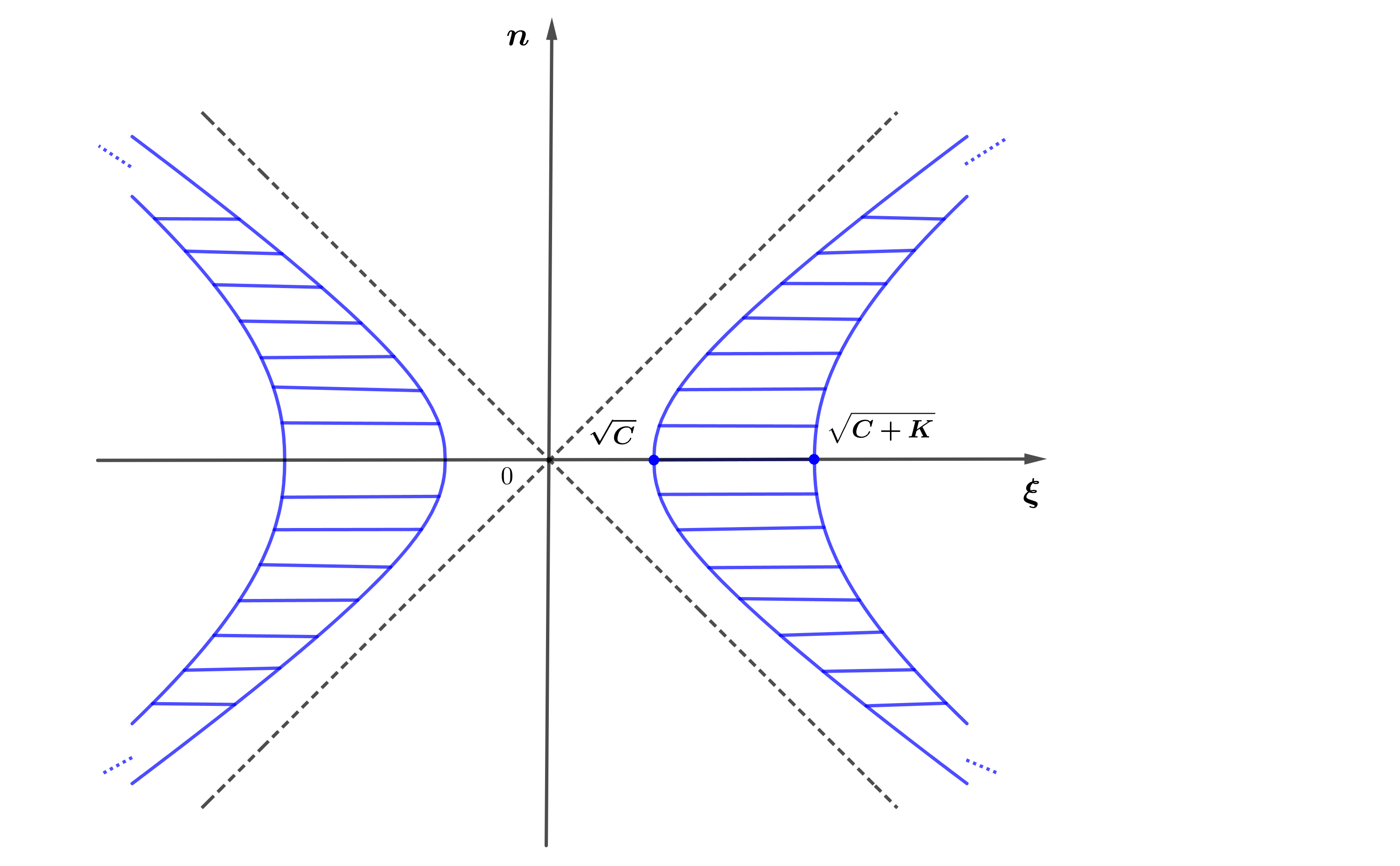
Figure 1. The dashed region represents the set $\mathcal{G}^{+}_{K}$ with $\alpha=1.3$ and $n_{0}=0$.

Note that for a fixed $n\in{\mathbb{Z}}$ we have

$$\mathfrak{m}\big{(}\big{\{}\xi\in{\mathbb{R}}:\xi^{2}-\tfrac{1}{2}\big{(}|n|^{2\alpha}+|n-n_{0}|^{2\alpha}\leq l\big{\}}\big{)}=2\sqrt{\tfrac{1}{2}\big{(}|n|^{2\alpha}+|n-n_{0}|^{2\alpha}\big{)}+l};$$

therefore

$$h(l)=2\displaystyle\sum_{n=0}^{\infty}\!\!\sqrt{\tfrac{1}{2}\big{(}|n|^{2\alpha}+|n-n_{0}|^{2\alpha}\big{)}+l}+2\displaystyle\sum_{n=1}^{\infty}\!\!\sqrt{\tfrac{1}{2}\big{(}|n|^{2\alpha}+|n+n_{0}|^{2\alpha}\big{)}+l}.$$ (2.26)

Then, from(2.25) and (2.26) it follows that

$$\mathfrak{m}\big{(}\mathcal{G}^{+}_{K}\big{)}=S_{1}^{+}+S_{2}^{+},$$ (2.27)

where

$$S_{1}^{+}=2\displaystyle\sum_{n=0}^{\infty}\!\!\sqrt{\tfrac{1}{2}\big{(}|n|^{2\alpha}+|n-n_{0}|^{2\alpha}\big{)}+C+K}-2\displaystyle\sum_{n=0}^{\infty}\!\!\sqrt{\tfrac{1}{2}\big{(}|n|^{2\alpha}+|n-n_{0}|^{2\alpha}\big{)}+C}$$

$$S_{2}^{+}=2\displaystyle\sum_{n=1}^{\infty}\!\!\sqrt{\tfrac{1}{2}\big{(}|n|^{2\alpha}+|n+n_{0}|^{2\alpha}\big{)}+C+K}-2\displaystyle\sum_{n=1}^{\infty}\!\!\sqrt{\tfrac{1}{2}\big{(}|n|^{2\alpha}+|n+n_{0}|^{2\alpha}\big{)}+C}.$$

For $S_{1}^{+}$ we have

$$\begin{split}S_{1}^{+}&=2\sum_{n=0}^{\infty}\frac{K}{\sqrt{\tfrac{1}{2}\big{(}|n|^{2\alpha}+|n-n_{0}|^{2\alpha}\big{)}+C+K}+\sqrt{\tfrac{1}{2}\big{(}|n|^{2\alpha}+|n-n_{0}|^{2\alpha}\big{)}+C}}\\ &\leq 2\sqrt{2}\sum_{n=0}^{\infty}\frac{K}{\sqrt{n^{2\alpha}+C+K}}\\ &\leq 2\sqrt{2}\Big{(}\frac{K}{\sqrt{C+K}}+K\sum_{n=1}^{\infty}\frac{1}{n^{\alpha}}\Big{)}\\ &\lesssim_{\alpha}K,\end{split}$$ (2.28)

where in the last estimate it has been used that $\alpha>1$ and $C+K\geq 1$. In a similar way one gets

$$S_{2}^{+}\lesssim_{\alpha}K.$$

Therefore, from (2.27) we have

$$\mathfrak{m}\big{(}\mathcal{G}^{+}_{K}\big{)}\lesssim_{\alpha}K.$$ (2.29)

Estimate of $\boldsymbol{\mathfrak{m}(\mathcal{G}_{K}^{-})}$. This case is more delicate. We write

$$\mathcal{G}_{K}^{-}=\Big{\{}(\xi,n)\in{\mathbb{R}}\times{\mathbb{Z}}:-(C+K)\leq\xi^{2}-\tfrac{1}{2}\big{(}|n|^{2\alpha}+|n-n_{0}|^{2\alpha}\big{)}\leq-C\Big{\}}$$ (2.30)

and observe that

$$\mathcal{G}_{K}^{-}\subset\mathcal{G}_{1,K}^{-}\cup\mathcal{G}_{2,K}^{-},$$ (2.31)

where

$$\mathcal{G}_{1,K}^{-}=\Big{\{}(\xi,n)\in{\mathbb{R}}\times{\mathbb{Z}}:|n-n_{0}|^{2\alpha}-(C+K)\leq\xi^{2}\leq|n|^{2\alpha}-C\Big{\}},$$

$$\mathcal{G}_{2,K}^{-}=\Big{\{}(\xi,n)\in{\mathbb{R}}\times{\mathbb{Z}}:|n|^{2\alpha}-(C+K)\leq\xi^{2}\leq|n-n_{0}|^{2\alpha}-C\Big{\}}.$$

Indeed, $\mathcal{G}_{1,K}^{-}$ contains the points of $\mathcal{G}_{K}^{-}$ with $|n-n_{0}|\leq|n|$ and $\mathcal{G}_{2,K}^{-}$ those that satisfy $|n-n_{0}|>|n|$.

Similar arguments to those used to estimate $\mathcal{G}_{K}^{+}$ give us

$$\begin{split}\mathfrak{m}\big{(}\mathcal{G}^{-}_{1,K}\big{)}&=4\Big{(}\sum_{n=\lfloor C^{\frac{1}{2\alpha}}\rfloor+1}^{\infty}\!\!\!\sqrt{n^{2\alpha}-C}\,\,\,-\!\!\!\sum_{n-n_{0}=\lfloor(C+K)^{\frac{1}{2\alpha}}\rfloor+1}^{\infty}\!\!\!\sqrt{(n-n_{0})^{2\alpha}-C-K}\Big{)}\\ &=4\Big{(}\sum_{n=\lfloor C^{\frac{1}{2\alpha}}\rfloor+1}^{\infty}\!\!\!\sqrt{n^{2\alpha}-C}\,\,\,-\!\!\!\sum_{n=\lfloor(C+K)^{\frac{1}{2\alpha}}\rfloor+1}^{\infty}\!\!\!\sqrt{n^{2\alpha}-C-K}\Big{)}\\ &:=4(S^{-}_{1}+S^{-}_{2}),\end{split}$$ (2.32)

where

$$S^{-}_{1} =\sum_{n=\lfloor C^{\frac{1}{2\alpha}}\rfloor+1}^{\lfloor(C+K)^{\frac{1}{2\alpha}}\rfloor}\sqrt{n^{2\alpha}-C},$$

$$S^{-}_{2} =\sum_{n=\lfloor(C+K)^{\frac{1}{2\alpha}}\rfloor+1}^{\infty}\big{(}\sqrt{n^{2\alpha}-C}-\sqrt{n^{2\alpha}-C-K}\big{)}.$$

To estimate $S_{1}^{-}$ we observe that

$$\begin{split}S^{-}_{1}&\leq\int_{C^{\frac{1}{2\alpha}}}^{\lfloor(C+K)^{\frac{1}{2\alpha}}\rfloor}\!\!\sqrt{z^{2\alpha}-C}\,dz+\sqrt{\lfloor(C+K)^{\frac{1}{2\alpha}}\rfloor^{2\alpha}-C}\\ &\leq\underbrace{\int_{C^{\frac{1}{2\alpha}}}^{(C+K)^{\frac{1}{2\alpha}}}\!\!\sqrt{z^{2\alpha}-C}\,dz}_{{\mathcal{J}}_{1}}+\sqrt{K}.\end{split}$$ (2.33)

To estimate the integral ${\mathcal{J}}_{1}$ we split the analysis into two cases.

Case: $\boldsymbol{C\geq 1}$. Using that $z\mapsto\sqrt{z^{2\alpha}-C}$ is an increasing function, we have

$${\mathcal{J}}_{1}\leq\sqrt{K}\big{(}(C+K)^{\frac{1}{2\alpha}}-C^{\frac{1}{2\alpha}}\big{)},$$

and applying the mean value theorem to the function $z\mapsto z^{\frac{1}{\alpha}}$ there exists $z^{*}\in\big{(}\sqrt{C},\,\sqrt{C+K}\big{)}$ such that

$$\begin{split}{\mathcal{J}}_{1}&\leq\sqrt{K}\frac{1}{\alpha\cdot(z^{*})^{1-\frac{1}{\alpha}}}\big{(}\sqrt{C+K}-\sqrt{C}\big{)}\\ &\leq\frac{\sqrt{K}}{\alpha C^{\frac{\alpha-1}{2\alpha}}}\frac{K}{\sqrt{C+K}+\sqrt{C}}\\ &\leq\frac{K}{\alpha},\end{split}$$ (2.34)

where in the last estimate it has been used that $C\geq 1$.

Case: $\boldsymbol{0<C<1}$. Using the change of variables $z=C^{\frac{1}{2\alpha}}\rho^{\frac{1}{\alpha}}$ and that the function $\rho\mapsto\sqrt{\rho^{2}-1}$ is increasing one gets

$$\begin{split}{\mathcal{J}}_{1}&=\frac{C^{\frac{1}{2}+\frac{1}{2\alpha}}}{\alpha}\int_{1}^{\sqrt{\frac{C+K}{C}}}\sqrt{\rho^{2}-1}\,\rho^{\frac{1}{\alpha}-1}\,d\rho\\ &\leq\frac{C^{\frac{1}{2\alpha}}}{\alpha}\sqrt{K}\int_{1}^{\sqrt{\frac{C+K}{C}}}\rho^{\frac{1}{\alpha}-1}\,d\rho\\ &\leq C^{\frac{1}{2\alpha}}\sqrt{K}\Big{(}\frac{C+K}{C}\Big{)}^{\frac{1}{2\alpha}}\\ &\lesssim\sqrt{K}(C+K)^{\frac{1}{2\alpha}}\\ &\lesssim K,\end{split}$$ (2.35)

where in the last estimate it has been used that $0<C<1$, $K\geq 1$ and $\alpha>1.$

Hence, from (2.33), (2.34) and (2.35) we have $S^{-}_{1}\lesssim_{\alpha}K.$

Now we estimate $S_{2}^{-}$ as follows

$$\begin{split}S^{-}_{2}&=\sum_{n=\lfloor(C+K)^{\frac{1}{2\alpha}}\rfloor+1}^{\infty}\frac{K}{\sqrt{n^{2\alpha}-C}+\sqrt{n^{2\alpha}-C-K}}\\ &\leq\sum_{n=\lfloor(C+K)^{\frac{1}{2\alpha}}\rfloor+1}^{\infty}\!\!\!\frac{K}{\sqrt{n^{2\alpha}-C}}\\ &\leq\frac{K}{\sqrt{\big{(}\lfloor(C+K)^{\frac{1}{2\alpha}}\rfloor+1\big{)}^{2\alpha}-C}}+\underbrace{\int_{(C+K)^{\frac{1}{2\alpha}}}^{\infty}\frac{K}{\sqrt{z^{2\alpha}-C}}dz}_{{\mathcal{J}}_{2}}\\ &\leq\sqrt{K}+{\mathcal{J}}_{2}\end{split}$$ (2.36)

and to estimate the integral ${\mathcal{J}}_{2}$, like in the case of ${\mathcal{J}}_{1}$, we split the analysis into two cases.

Case: $\boldsymbol{C\geq 1}$. Using the change of variable $z=C^{\frac{1}{2\alpha}}\rho^{\frac{1}{\alpha}}$ with $\alpha>1$ we have

$$\begin{split}{\mathcal{J}}_{2}&=\frac{K}{C^{\frac{1}{2}-\frac{1}{2\alpha}}}\int_{\sqrt{\frac{C+K}{C}}}^{\infty}\frac{d\rho}{\sqrt{\rho^{2}-1}\,\rho^{1-\frac{1}{\alpha}}}\\ &\leq K\int_{1}^{\infty}\frac{d\rho}{\sqrt{\rho^{2}-1}\,\rho^{1-\frac{1}{\alpha}}}\\ &=K\Big{(}\int_{1}^{2}\frac{d\rho}{\sqrt{\rho-1}\sqrt{\rho+1}\,\rho^{1-\frac{1}{\alpha}}}+\int_{2}^{\infty}\frac{d\rho}{\sqrt{\rho^{2}-1}\,\rho^{1-\frac{1}{\alpha}}}\Big{)}\\ &\lesssim K\Big{(}\int_{1}^{2}\frac{d\rho}{\sqrt{\rho-1}}+\int_{2}^{\infty}\frac{d\rho}{\rho^{2-\frac{1}{\alpha}}}\Big{)}\\ &\lesssim_{\alpha}K\end{split}$$ (2.37)

Case: $\boldsymbol{0<C<1}$. In this case, since $K\geq 1$, we have

$${\mathcal{J}}_{2}\leq K\int_{1}^{\infty}\frac{dz}{\sqrt{z^{2\alpha}-1}}.$$

Then, using now the change of variable $z=\rho^{\frac{1}{\alpha}}$ and that $\alpha>1$, one gets

$${\mathcal{J}}_{2}\leq K\int_{1}^{\infty}\frac{d\rho}{\sqrt{\rho^{2}-1}\,\rho^{1-\frac{1}{\alpha}}}\lesssim_{\alpha}K,$$ (2.38)

as showed in the case $C\leq 1.$

Then, inserting (2.37) and (2.38) in (2.36) one gets $S^{-}_{2}\lesssim_{\alpha}K.$ Therefore, from (2.32) and the estimates obtained for $S^{-}_{1}$ and $S^{-}_{2}$ we have

$$\mathfrak{m}\big{(}\mathcal{G}^{-}_{1,K}\big{)}\lesssim_{\alpha}K.$$

By the same way we have $\mathfrak{m}\big{(}\mathcal{G}^{-}_{2,K}\big{)}\lesssim_{\alpha}K.$ So,

$$\mathfrak{m}\big{(}\mathcal{G}^{-}_{K}\big{)}\leq\mathfrak{m}\big{(}\mathcal{G}^{-}_{1,K}\big{)}+\mathfrak{m}\big{(}\mathcal{G}^{-}_{2,K}\big{)}\lesssim_{\alpha}K,$$

which joint with (2.29) give us (2.19). This completes the proof of Lemma 2.1. ∎

Remark 2.2.

For the case $0<\alpha\leq 1$ the result stated in Lemma 2.1 fails. Indeed, the series $S_{1}^{+}$ in (2.28) diverges for all $0<\alpha\leq 1$.

Proposition 2.3 (hyperbolic bilinear estimate).

Let $u_{1}$ and $u_{2}$ be two functions on $L^{2}({\mathbb{R}}\times{\mathbb{R}}\times{\mathbb{T}})$ with the following support properties:

$$\text{supp}\,(\widehat{u_{j}})\subseteq\mathcal{H}^{-}_{K_{j}},~{}~{}j=1,2,$$

where

$$\mathcal{H}^{-}_{K_{j}}:=\Big{\{}(\tau;\xi,n):\tfrac{1}{2}K_{j}\leq|\tau+\xi^{2}-|n|^{2\alpha}|\leq 2K_{j}\Big{\}}.$$ (2.39)

Then we have the following inequality

$$\|u_{1}u_{2}\|_{L^{2}({\mathbb{R}}\times{\mathbb{R}}\times\mathbb{T})}\lesssim(K_{1}K_{2})^{\frac{1}{2}}~{}\|u_{1}\|_{L^{2}({\mathbb{R}}\times{\mathbb{R}}\times\mathbb{T})}~{}\|u_{2}\|_{L^{2}({\mathbb{R}}\times{\mathbb{R}}\times\mathbb{T})}.$$ (2.40)

Proof.

Using the Cauchy-Schwarz inequality and Plancherel’s theorem we have

$$\begin{split}\|u_{1}u_{2}\|_{L^{2}_{txy}}^{2}&=\int_{-\infty}^{\infty}\int_{-\infty}^{\infty}\sum_{n\in{\mathbb{Z}}}\Big{|}\int_{-\infty}^{\infty}\int_{-\infty}^{\infty}\sum_{n_{1}\in{\mathbb{Z}}}\mathds{1}_{{\mathcal{A}}_{\tau\xi n}}(\tau_{1};\xi_{1},n_{1})\cdot\widehat{u_{1}}(\tau_{1};\xi_{1},n_{1})\\ &\hskip 142.26378pt\cdot\widehat{u_{2}}(\tau-\tau_{1};\xi-\xi_{1},n-n_{1})d\xi_{1}d\tau_{1}\Big{|}^{2}d\xi d\tau\\ &\lesssim\underset{\tau,\xi,n}{\mbox{sup}}\,\mathfrak{m}({\mathcal{A}}_{\tau\xi n})\|u_{1}\|^{2}_{L^{2}_{txy}}\|u_{2}\|^{2}_{L^{2}_{txy}},\end{split}$$ (2.41)

where

$${\mathcal{A}}_{\tau,\xi,n}:=\Big{\{}(\tau_{1};\xi_{1},n_{1}):(\tau_{1};\xi_{1},n_{1})\in\mbox{supp}\,(\widehat{u_{1}})~{}\text{and}~{}(\tau-\tau_{1};\xi-\xi_{1},n-n_{1})\in\mbox{supp}\,(\widehat{u_{2}})\Big{\}}.$$

Notice that if $(\tau_{1};\xi_{1},n_{1})\in{\mathcal{A}}_{\tau,\xi,n}$, then

$$\tau_{1}\in J_{1}:=\big{[}a_{1}-2K_{1},\,a_{1}+2K_{1}\big{]}\quad\text{and}\quad\tau_{1}\in J_{2}:=\big{[}a_{2}-2K_{2},\,a_{2}+2K_{2}\big{]},$$

where $a_{1}=|n_{1}|^{2\alpha}-\xi_{1}^{2}$ and $a_{2}=\tau+(\xi-\xi_{1})^{2}-|n-n_{1}|^{2\alpha}$. Hence

$$\tau_{1}\in J_{1}\cap J_{2},\;\text{with}\;|J_{1}\cap J_{2}|\leq 4\min\{K_{1},K_{2}\}.$$ (2.42)

On the other hand, for all $(\tau_{1};\xi_{1},n_{1})\in{\mathcal{A}}_{\tau,\xi,n}$ we can use the triangle inequality to eliminate $\tau_{1}$ to get

$$\begin{split}\Big{|}(\xi_{1}-\tfrac{\xi}{2})^{2}-\tfrac{1}{2}\big{(}|n_{1}|^{2\alpha}&+|n-n_{1}|^{2\alpha}\big{)}+\tfrac{\tau}{2}+\tfrac{\xi^{2}}{4}\Big{|}\\ &=\frac{1}{2}\big{|}\tau+\xi_{1}^{2}-|n_{1}|^{2\alpha}+(\xi-\xi_{1})^{2}-|n-n_{1}|^{2\alpha}\big{|}\\ &\leq\tfrac{1}{2}\Big{(}\big{|}\tau_{1}+\xi_{1}^{2}-|n_{1}|^{2\alpha}\big{|}+\big{|}\tau-\tau_{1}+(\xi-\xi_{1})^{2}-|n-n_{1}|^{2\alpha}\big{|}\Big{)}\\ &<K_{1}+K_{2}.\end{split}$$ (2.43)

So,

$$\text{if}\;(\tau_{1};\xi_{1},n_{1})\in{\mathcal{A}}_{\tau,\xi,n},\;\text{then}\;(\xi_{1},n_{1})\in{\mathcal{B}}_{\tau,\xi,n},$$ (2.44)

where

$${\mathcal{B}}_{\tau,\xi,n}\in{\mathbb{R}}\times{\mathbb{Z}}:=\Big{\{}(\xi_{1},n_{1}):\big{|}(\xi_{1}-\tfrac{\xi}{2})^{2}-\tfrac{1}{2}\big{(}|n_{1}|^{2\alpha}+|n_{1}-n|^{2\alpha}\big{)}+\tfrac{\tau}{2}+\tfrac{\xi^{2}}{4}\big{|}\leq K_{1}+K_{2}\Big{\}}.$$

Now, note that

$${\mathcal{B}}_{\tau,\xi,n}\subset\Big{\{}(\xi_{1},n_{1})\in{\mathbb{R}}\times{\mathbb{Z}}:C\leq\big{|}(\xi_{1}-\tfrac{\xi}{2})^{2}-\tfrac{1}{2}\big{(}|n_{1}|^{2\alpha}+|n_{1}-n|^{2\alpha}\big{)}\big{|}\leq C+2(K_{1}+K_{2})\Big{\}}$$

with $C=\big{|}\tfrac{\tau}{2}-\tfrac{\xi^{2}}{4}\big{|}-(K_{1}+K_{2}).$ Hence, if $C>0$ we use Lemma 2.1 (with $\xi_{0}=\tfrac{\xi}{2}$ and $n_{0}=n$) to get

$$\mathfrak{m}({\mathcal{B}}_{\tau,\xi,n})\lesssim K_{1}+K_{2}.$$

Otherwise, if $C<0$ we have

$$\begin{split}\mathfrak{m}({\mathcal{B}}_{\tau,\xi,n})&\leq\mathfrak{m}\Big{(}\Big{\{}(\xi_{1},n_{1}):\big{|}(\xi_{1}-\tfrac{\xi}{2})^{2}-\tfrac{1}{2}\big{(}|n_{1}|^{2\alpha}+|n_{1}-n|^{2\alpha}\big{)}\big{|}\leq 2(K_{1}+K_{2})\Big{\}}\Big{)}\\ &=\lim\limits_{\varepsilon\searrow 0}\mathfrak{m}\Big{(}\Big{\{}(\xi_{1},n_{1}):\varepsilon<\big{|}(\xi_{1}-\tfrac{\xi}{2})^{2}-\tfrac{1}{2}\big{(}|n_{1}|^{2\alpha}+|n_{1}-n|^{2\alpha}\big{)}\big{|}\leq 2(K_{1}+K_{2})\Big{\}}\Big{)}\\ &\lesssim K_{1}+K_{2},\end{split}$$ (2.45)

where in the last estimate it was used again the Lemma 2.1.

Finally, collecting the information in (2.42), (2.44) and (2.45) one gets

$$\mathfrak{m}({\mathcal{A}}_{\tau,\xi,n})\leq|J_{1}\cap J_{2}|\cdot\mathfrak{m}({\mathcal{B}}_{\tau,\xi,n})\lesssim\min\{K_{1},K_{2}\}\max\{K_{1},K_{2}\}$$

and inserting this in (2.41) we obtain

$$\|u_{1}u_{2}\|_{L^{2}_{txy}}^{2}\lesssim K_{1}K_{2}\|u_{1}\|^{2}_{L^{2}_{txy}}\|u_{2}\|^{2}_{L^{2}_{txy}}.$$

Then, the result is proved. ∎

3. Bilinear estimate in the elliptic case

Now we prove the corresponding bilinear estimate for the elliptic symbol of the operator.

Lemma 3.1.

Let $\alpha\geq 1$, $\xi_{0}\in{\mathbb{R}}$, $n_{0}\in{\mathbb{Z}}$ and $C\geq 1$. Then for all $K\geq 1$, the set

$$\widetilde{\mathcal{G}}_{K}:=\Big{\{}(\xi,n)\in{\mathbb{R}}\times{\mathbb{Z}}:C\leq(\xi-\xi_{0})^{2}+\tfrac{1}{2}\big{(}|n|^{2\alpha}+|n-n_{0}|^{2\alpha}\big{)}\leq C+K\Big{\}}$$

satisfies the estimate

$$\sup\limits_{(\xi_{0},n_{0},C)\in\Lambda}\mathfrak{m}(\widetilde{\mathcal{G}}_{K})\lesssim_{\alpha}K,$$ (3.46)

where $\Lambda:={\mathbb{R}}\times{\mathbb{Z}}\times{\mathbb{R}}^{+}$.

Proof.

As in Lemma 2.1 it suffices to consider the case $\xi_{0}=0$. For all $K\geq 1$ notice that

$$\widetilde{\mathcal{G}}_{K}\subset\widetilde{\mathcal{G}}_{1,K}\cup\widetilde{\mathcal{G}}_{2,K},$$ (3.47)

where

$$\widetilde{\mathcal{G}}_{1,K}=\Big{\{}(\xi,n)\in{\mathbb{R}}\times{\mathbb{Z}}:C-|n|^{2\alpha}\leq\xi^{2}\leq C+K-|n-n_{0}|^{2\alpha}\Big{\}},$$

$$\widetilde{\mathcal{G}}_{2,K}=\Big{\{}(\xi,n)\in{\mathbb{R}}\times{\mathbb{Z}}:C-|n-n_{0}|^{2\alpha}\leq\xi^{2}\leq C+K-|n|^{2\alpha}\Big{\}}.$$

Indeed, $\widetilde{\mathcal{G}}_{1,K}$ contains the points of $\widetilde{\mathcal{G}}_{K}$ with $|n-n_{0}|\leq|n|$ and $\widetilde{\mathcal{G}}_{2,K}$ those that satisfy $|n-n_{0}|>|n|$.

Similar analysis as performed in the hyperbolic case shows that

$$\begin{split}\mathfrak{m}(\widetilde{\mathcal{G}}_{1,K})&=2\sum\limits_{|n-n_{0}|=0}^{\lfloor(C+K)^{\frac{1}{2\alpha}}\rfloor}\sqrt{C+K-|n-n_{0}|^{2\alpha}}-2\sum\limits_{|n|=0}^{\lfloor C^{\frac{1}{2\alpha}}\rfloor}\sqrt{C-|n|^{2\alpha}}\\ &=2\sum\limits_{|n|=0}^{\lfloor(C+K)^{\frac{1}{2\alpha}}\rfloor}\sqrt{C+K-|n|^{2\alpha}}-2\sum\limits_{|n|=0}^{\lfloor C^{\frac{1}{2\alpha}}\rfloor}\sqrt{C-|n|^{2\alpha}}\\ &:=\widetilde{S}_{1}+\widetilde{S}_{2},\end{split}$$ (3.48)

where

$$\widetilde{S}_{1} =2\sum\limits_{|n|=0}^{\lfloor C^{\frac{1}{2\alpha}}\rfloor}\Big{(}\sqrt{C+K-|n|^{2\alpha}}-\sqrt{C-|n|^{2\alpha}}\Big{)},$$

$$\widetilde{S}_{2} =2\sum\limits_{|n|=\lfloor C^{\frac{1}{2\alpha}}\rfloor+1}^{\lfloor(C+K)^{\frac{1}{2\alpha}}\rfloor}\sqrt{C+K-|n|^{2\alpha}}.$$

In order to estimate $\widetilde{S}_{1}$ we use that

$$\begin{split}\widetilde{S}_{1}&=2\sum\limits_{|n|=0}^{\lfloor C^{\frac{1}{2\alpha}}\rfloor}\frac{K}{\Big{(}\sqrt{C+K-|n|^{2\alpha}}+\sqrt{C-|n|^{2\alpha}}\Big{)}}\\ &\leq 2\sum\limits_{|n|=0}^{\lfloor C^{\frac{1}{2\alpha}}\rfloor-1}\frac{K}{\sqrt{C-|n|^{2\alpha}}}+\frac{2K}{\sqrt{C+K-\lfloor C^{\frac{1}{2\alpha}}\rfloor^{2\alpha}}}\\ &\leq 4K\int_{0}^{C^{\frac{1}{2\alpha}}}\frac{dz}{\sqrt{C-z^{2\alpha}}}+2\sqrt{K}.\end{split}$$ (3.49)

Making now the change of variables $z=C^{\frac{1}{2\alpha}}\rho^{\frac{1}{\alpha}}$ with $\alpha\geq 1$ we have from (3.49)

$$\begin{split}\widetilde{S}_{1}&\leq\frac{4K}{\alpha C^{\frac{\alpha-1}{2\alpha}}}\int_{0}^{1}\frac{d\rho}{\rho^{1-\frac{1}{\alpha}}\sqrt{1-\rho^{2}}}+2\sqrt{K}\\ &\lesssim\frac{4K}{\alpha C^{\frac{\alpha-1}{2\alpha}}}\Big{(}\int_{0}^{1}\frac{d\rho}{\rho^{1-\frac{1}{\alpha}}}+\int_{0}^{1}\frac{d\rho}{\sqrt{1-\rho^{2}}}\Big{)}+2\sqrt{K}\\ &\lesssim_{\alpha}K,\end{split}$$ (3.50)

where it has been used that $C\geq 1$ and $\alpha\geq 1$.

Now we proceed to estimate $\widetilde{S}_{2}$. First note that

$$\begin{split}\widetilde{S}_{2}&=4\sum\limits_{n=\lfloor C^{\frac{1}{2\alpha}}\rfloor+1}^{\lfloor(C+K)^{\frac{1}{2\alpha}}\rfloor}\sqrt{C+K-n^{2\alpha}}\\ &\leq 4\sqrt{K}+\int_{\lfloor C^{\frac{1}{2\alpha}}\rfloor+1}^{\lfloor(C+K)^{\frac{1}{2\alpha}}\rfloor}\sqrt{C+K-z^{2\alpha}}dz\\ &\leq 4\sqrt{K}+\int_{C^{\frac{1}{2\alpha}}}^{(C+K)^{\frac{1}{2\alpha}}}\sqrt{C+K-z^{2\alpha}}dz\\ &\leq 4\sqrt{K}+\sqrt{K}\big{(}(C+K)^{\frac{1}{2\alpha}}-C^{\frac{1}{2\alpha}}\big{)}.\end{split}$$ (3.51)

The same arguments to get (2.34) give us that

$$(C+K)^{\frac{1}{2\alpha}}-C^{\frac{1}{2\alpha}}\leq\frac{1}{\alpha C^{\frac{\alpha-1}{2\alpha}}}\frac{K}{\sqrt{C+K}+\sqrt{C}}\leq\frac{K}{\alpha}$$ (3.52)

for all $C\geq 1$ and $\alpha\geq 1$. Combining (3.51) and (3.52) we have

$$\widetilde{S}_{2}\lesssim_{\alpha}K,$$

then the proof is finished. ∎

Remark 3.2.

For the case $0<\alpha<1$ the result stated in Lemma 3.1 fails. Indeed, it is not difficult to see that the $\widetilde{S}_{1}$ verifies (3.50) in the following way

$$\widetilde{S}_{1}\sim\Big{(}\frac{1}{C^{\frac{\alpha-1}{2\alpha}}}+1\Big{)}K,$$

where $\frac{1}{C^{\frac{\alpha-1}{2\alpha}}}\to+\infty$ as $C\to+\infty$ whenever $0<\alpha<1$.

In the same way as in the hyperbolic case, Lemma 3.1 implies the following result.

Proposition 3.3 (elliptic bilinear estimate).

Let $u_{1}$ and $u_{2}$ be two functions on $L^{2}({\mathbb{R}}\times{\mathbb{R}}\times{\mathbb{T}})$ with the following support properties:

$$\text{supp}\,(\widehat{u_{j}})\subseteq\mathcal{H}^{+}_{K_{j}},~{}~{}j=1,2,$$

where

$$\mathcal{H}^{+}_{K_{j}}:=\Big{\{}(\tau;\xi,n):\tfrac{1}{2}K_{j}\leq|\tau+\xi^{2}+|n|^{2\alpha}|\leq 2K_{j}\Big{\}}.$$ (3.53)

Then we have the following inequality

$$\|u_{1}u_{2}\|_{L^{2}({\mathbb{R}}\times{\mathbb{R}}\times\mathbb{T})}\lesssim(K_{1}K_{2})^{\frac{1}{2}}~{}\|u_{1}\|_{L^{2}({\mathbb{R}}\times{\mathbb{R}}\times\mathbb{T})}~{}\|u_{2}\|_{L^{2}({\mathbb{R}}\times{\mathbb{R}}\times\mathbb{T})}.$$ (3.54)

4. Strichartz Inequality on ${\mathbb{R}}\times{\mathbb{T}}$

This section is devoted to the proof of Theorem  1.2, which follows the same lines as previous proofs of related results in [15] and we reproduce an sketch of it for the sake of completeness.

4.1. Proof of Theorem  1.2–(1.14)

The first step is the proof of the following $L^{4}$ Strichartz estimate in the Bourgain space $X_{\alpha\pm}^{b,0}$.

Step 1. Let $\alpha\geq 1$ in the case (+), $\alpha>1$ in the case (-) and $b>1/2$. Then we have

$$\|u\|_{L^{4}({\mathbb{R}}\times{\mathbb{R}}\times\mathbb{T})}\lesssim\|u\|_{X_{\alpha\pm}^{b,0}({\mathbb{R}}\times{\mathbb{R}}\times\mathbb{T})}$$ (4.55)

for any $u\in X_{\alpha\pm}^{b,0}({\mathbb{R}}\times{\mathbb{R}}\times\mathbb{T})$.

Proof of Step 1. Let $u$ a smooth function and consider the dyadic decomposition

$$u(t;x,y)=\sum_{k=0}^{\infty}u_{2^{k}}(t;x,y),$$

with $\text{supp}(\widehat{u_{2^{k}}})\in\mathcal{H}^{\pm}_{2^{k}}$ defined in (2.39). Using Proposition 2.3, Proposition 3.3 and that $b>1/2$ one gets

$$\begin{split}\|u\|^{2}_{L^{4}({\mathbb{R}}\times{\mathbb{R}}\times\mathbb{T})}&=\|uu\|_{L^{2}({\mathbb{R}}\times{\mathbb{R}}\times\mathbb{T})}\\ &\leq\sum_{k_{1}=0}^{\infty}\sum_{k_{2}=0}^{\infty}\|u_{2^{k_{1}}}u_{2^{k_{2}}}\|_{L^{2}({\mathbb{R}}\times{\mathbb{R}}\times\mathbb{T})}\\ &\lesssim\sum_{k_{1}=0}^{\infty}\sum_{k_{2}=0}^{\infty}(2^{k_{1}}2^{k_{2}})^{1/2}\|\widehat{u_{2^{k_{1}}}}\|_{L^{2}({\mathbb{R}}\times{\mathbb{R}}\times\mathbb{T})}\|\widehat{u_{2^{k_{2}}}}\|_{L^{2}({\mathbb{R}}\times{\mathbb{R}}\times\mathbb{T})}\\ &\lesssim\sum_{k_{1}=0}^{\infty}(2^{k_{1}})^{1/2-b}\sum_{k_{2}=0}^{\infty}(2^{k_{2}})^{1/2-b}\|u\|^{2}_{X_{\alpha^{\pm}}^{b,0}}\\ &\lesssim\|u\|^{2}_{X_{\alpha\pm}^{b,0}},\end{split}$$

as claimed in (4.55).

Step 2. Let $0<\delta\leq 1$ and $I=[-\delta,\delta]$. Then,

$$\|U^{\pm}_{\alpha}(t)\phi\|_{L^{4}(I\times{\mathbb{R}}\times{\mathbb{T}})}\lesssim(\delta^{1/2}+\delta^{1/2-b})\|\phi\|_{L^{2}({\mathbb{R}}\times{\mathbb{T}})},$$ (4.56)

for any $b>0$.

Proof of Step 2. Let $\psi\in C^{\infty}_{0}$ be a cut-off function such that $\mbox{supp~{}}(\psi)\subset(-2,2)$ and $\psi(t)\equiv 1$ on $[-1,1]$ and define $\psi_{\delta}(t):=\psi(\frac{t}{\delta})$. For $b>0$, one gets

$$\|\psi_{\delta}\|_{H^{b}_{t}}\lesssim\delta^{1/2}\|\psi\|_{L^{2}_{t}}+\delta^{1/2-b}\|\psi\|_{\dot{H}^{b}_{t}}.$$

Now, applying (4.55), we have

$$\begin{split}\|U^{\pm}_{\alpha}(t)\phi\|_{L^{4}(I\times{\mathbb{R}}\times{\mathbb{T}})}&\lesssim\|\psi_{\delta}(t)U^{\pm}_{\alpha}(t)\phi\|_{L^{4}({\mathbb{R}}\times{\mathbb{R}}\times{\mathbb{T}})}\\ &\lesssim\|\psi_{\delta}(t)U^{\pm}_{\alpha}(t)\phi\|_{X^{b,0}_{\alpha^{\pm}}({\mathbb{R}}\times{\mathbb{R}}\times\mathbb{T})}\\ &=\|\psi_{\delta}\|_{H^{b}_{t}}\|\phi\|_{L^{2}({\mathbb{R}}\times{\mathbb{T}})}\\ &\lesssim(\delta^{1/2}+\delta^{1/2-b})\|\phi\|_{L^{2}({\mathbb{R}}\times{\mathbb{T}})},\end{split}$$

so (4.56) is proved.

Finally, the estimate (4.56) can be extended to an arbitrary interval $I$ in the same way as in [15]. This completes the proof of Theorem  1.2–(1.14).

4.2. Proof of Theorem  1.2–(1.15)

Consider the linear operator $A:L^{2}({\mathbb{R}}\times\mathbb{T})\to L^{4}(I\times{\mathbb{R}}\times\mathbb{T})$, defined by $A\phi:=U^{\pm}_{\alpha}(t)\phi$. Due to the estimate (1.14) we observe that $A$ is bounded. Let us denote by $A^{*}$ the adjoint operator of $A$, then

$$A^{*}(f)=\displaystyle\int_{I}U^{\pm}_{\alpha}(-t^{\prime})f(t^{\prime};\cdot)dt^{\prime},$$

which is bounded from $L^{4/3}(I\times{\mathbb{R}}\times\mathbb{T})$ to $L^{2}({\mathbb{R}}\times\mathbb{T})$, i.e.,

$$\left\|\int_{I}U^{\pm}_{\alpha}(-t^{\prime})f(t^{\prime};\cdot)dt^{\prime}\right\|_{L^{2}({\mathbb{R}}\times\mathbb{T})}\leq C^{*}_{I}\left\|f\right\|_{L^{4/3}(I\times{\mathbb{R}}\times\mathbb{T})}$$

for some constant $C^{*}_{I}$, depending only on the measure of $I$. Therefore,

$$AA^{*}=\displaystyle\int_{I}U^{\pm}_{\alpha}(t-t^{\prime})f(t^{\prime};\cdot)dt^{\prime},$$

is bounded from $L^{4/3}(I\times{\mathbb{R}}\times\mathbb{T})$ to $L^{4}(I\times{\mathbb{R}}\times\mathbb{T})$, satisfying

$$\left\|\int_{I}U^{\pm}_{\alpha}(t-t^{\prime})f(t^{\prime};\cdot)dt^{\prime}\right\|_{L^{4}(I\times{\mathbb{R}}\times\mathbb{T})}\leq C_{I}C^{*}_{I}\left\|f\right\|_{L^{4/3}(I\times{\mathbb{R}}\times\mathbb{T})}.$$

Finally, to complete the proof of (1.15) is used the arguments in Lemma 3.1 of [13].

References

- [1] J. Bourgain; Fourier transform restriction phenomena for certain lattice subsets and application to nonlinear evolution equations I, Schrödinger equations. Geom. Funct. Anal. 3, 107-156 (1993).
- [2] J. Bourgain; Global Solutions of Nonlinear Schrödinger Equations. AMS Colloquium Publications, Vol. 46, Amer. Math. Soc., Providence, RI (1999).
- [3] T. Cazenave and F.Weissler; Some Remarks on the Nonlinear Schrd̈inger Equation in the Critical Case. Lecture Notes in Math. 1394, Springer, Berlin, 18?29 (1989).
- [4] D. R. Crawford, P. G. Saffman, H. C. Yuen; Evolution of a random inhomogeneous field of nonlinear deep-wave gravity waves. Wave Motion 2, 1-16 (1980).
- [5] A. DeBouard; Analytic solution to non elliptic non linear Schrödinger equations. J. Differential Equations 104, , 196-213 (1993).
- [6] J.M. Ghidaglia and J.C. Saut; On the initial value problem for the Davey-Stewartson systems. Nonlinearity 3, 475-506 (1990).
- [7] S. Herr, D. Tataru and N. Tzvetkov; Strichartz estimates for partially periodic solutions to Schrödinger equations in and applications. Journal für die reine und angewandte Mathematik (Crelles Journal) 2014 (690), 65-78 (2014).
- [8] C. E. Kenig, G. Ponce and L. Vega; On the ill-posedness of some canonical dispersive equations, Duke Math. J. 106 3 (2001), 617–633.
- [9] E. A. Kuznetsov, S. K. Turitsyn; Talanov transformations in self-focusing problems and instability of stationary waveguides. Physics Letters 112, 273-275 (1985).
- [10] A.C. Newell; Solitons in Mathematics and Physics. Regional Conference series in Applied Math. 48, SIAM (1985).
- [11] T. Oh; A remark on norm inflation with general initial data for the cubic nonlinear Schrödinger equations in negative Sobolev spaces. Funkcial. Ekvac. 60, 259-277 (2017).
- [12] A. Scott, F. Chu, and D. McLaughlin; The soliton: a new concept in applied science. Proc. IEEE 97, 1143-1183 (1973).
- [13] H.F. Smith and C.D. Sogge; Global Strichartz estimates for nonthapping perturbations of the laplacian: Estimates for nonthapping perturbations. Communications in Partial Differential Equations 25, 2171-2183 (2000).
- [14] C. Sulem, P.-L. Sulem; The Nonlinear Schrödinger Equation. Self-focusing and Wave Collapse. Appl. Math. Sci., 139, Springer (1999).
- [15] H. Takaoka and N. Tzvetkov; On 2D Nonlinear Schrödinger Equation with Data on . Journal of Functional Analysis 182, 427-442 (2001).
- [16] Y. Wang; Periodic cubic Hyperbolic Schrödinger equation on . Jornal of Functionl Analysis 265, 424-434 (2013).
- [17] V.E. Zakharov and A.B. Shabat; Exact theory of two dimensional self modulation of waves in nonlinear media. Sov. Phys. J.E.T.P. 34, 62-69 (1972).