Not all layers are equally as important: Every Layer Counts BERT

Abstract

This paper introduces a novel modification of the transformer architecture, tailored for the data-efficient pretraining of language models. This aspect is evaluated by participating in the BabyLM challenge, where our solution won both the strict and strict-small tracks. Our approach allows each transformer layer to select which outputs of previous layers to process. The empirical results verify the potential of this simple modification and show that not all layers are equally as important.

1 Introduction

Modern language models (LLMs), with their deep architectures and large parameter counts, have displayed outstanding performance on a wide range of tasks. Their ability to understand, generate, and manipulate human language has been groundbreaking (Devlin et al., 2019; Raffel et al., 2020; Brown et al., 2020). However, this success largely relies on vast amounts of unsupervised data that these models need for pretraining, requiring extensive computational power and time. While this is feasible for high-resource languages like English, it becomes a bottleneck for languages with limited data resources (Joshi et al., 2020). Moreover, the environmental and economic costs of such massive training regimens are growing concerns (Strubell et al., 2019; Thompson et al., 2020).

The BabyLM challenge tries to address these concerns by providing a shared experimental ground for efficient language modelling (Warstadt et al., 2023). All models submitted to this shared task have to be trained on a restricted text corpus of 10M and 100M words – in the strict-small and strict tracks, respectively. The challenge pushes the boundaries of what is possible with data-efficient language model pretraining.

strict-small track (10M words)
Model	BLiMP	GLUE	MSGS	Average
ELC-BERT (ours)	75.8	73.7	29.4	65.9
MLSM	72.4	70.6	17.2	60.8
Contextualizer	74.3	69.6	12.7	60.5
Baby Llama	69.8	67.6	24.7	60.1
Too Much Information	75.7	70.9	3.9	59.9
strict track (100M words)
Model	BLiMP	GLUE	MSGS	Average
ELC-BERT (ours)	82.8	78.3	47.2	74.3
Contextualizer	79.0	72.9	58.0	73.0
BootBERT	82.2	78.5	27.7	70.2
MSLM	76.2	73.5	21.4	64.4
Bad babies	77.0	67.2	23.4	63.4

Table 1: The DynaBench scores of the BabyLM challenge (Warstadt et al., 2023), the table shows the top 5 submissions in the strict-small and strict tracks. Higher scores are better, the best results in each evaluation suite are boldfaced.

In response to this challenge, we present a novel modification to the well-established transformer architecture (Vaswani et al., 2017). Instead of traditional residual connections, our model allows each layer to selectively process outputs from the preceding layers. This flexibility leads to intriguing findings: not every layer is of equal significance to the following layers. Thus, we call it the ‘Every Layer Counts’ BERT (ELC-BERT).

The BabyLM challenge provided us with a robust benchmark to evaluate the efficacy of ELC-BERT. Our approach emerged as the winning submission in both the strict and strict-small tracks (Table 1), which highlights the potential of layer weighting for future low-resource language modelling.

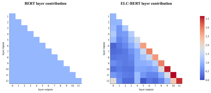
Figure 1: Every layer can select which outputs from previous layers it wants as its input, these heatmaps show the weights given to each previous layer output. The unit weights of the BERT model (and of any standard transformer-based model) are inferred from Equation 4. The right heatmap shows the $\alpha$ weights of the normalized ELC-BERT variant; for clear visual comparison between the two models, we rescale the $\alpha$ weights so that the $k$th row sums to $k$. Note that the layer 0 is the embedding layer, as in Equation 1.

Transparent and open-source language modelling is necessary for safe future development of this field. We release the full source code, together with the pre-trained ELC-BERT models, online.

2 Related work

Residual and highway networks.

While the predecessor of residual models, highway networks, used a conditional gating mechanism to weigh layers (Srivastava et al., 2015), modern residual networks (including transformers) simply weigh all layers equally (He et al., 2016; Vaswani et al., 2017). Our work reintroduces layer weights into residual models – but without the computational cost of a gating mechanism.

Layer importance.

The difference between various layers inside pre-trained language models has been extensively studied (Jawahar et al., 2019; Tenney et al., 2019; Niu et al., 2022). Different layers process different linguistic phenomena, thus their importance for downstream tasks varies – this has been successfully utilized by learning layer weights during finetuning, for example in ULMFiT (Howard and Ruder, 2018) or UDify (Kondratyuk and Straka, 2019). Following this direction, our system uses layer weights in the finetuning as well as in the pretraining phase.

ReZero transformer.

A related approach to ours was proposed by Bachlechner et al. (2021). In that paper, the authors experimented with scaling the output of each layer. They showed that by initializing the scaling parameter to zero, their ‘ReZero transformer’ model tends towards setting the scale to $\nicefrac{{1}}{{N}}$ (where $N$ is the number of layers). Our approach can be considered as a generalization of this method – in ELC-BERT, every layer weights the outputs of previous layers individually.

3 ELC-BERT layer weighting

We modify the residual connections inside the transformer architecture so that every layer can select which outputs from previous layers it wants to process – instead of always taking a simple sum of all preceding layers, as done in the Transformer (Vaswani et al., 2017) and in most works that use a variant of this architecture. This modification allows the model to form a complex inter-layer structure, as visible from Figure 1.

Transformer definition.

To be more specific, we first formally define a transformer encoder as a function that maps subword indices $\bm{x}$ onto subword probabilities $\bm{y}$. First, $\bm{x}$ is embedded into a vector representation $\bm{h}^{0}_{\text{out}}$, which is then processed by $N$ layers consisting of attention and multi-layer-perceptron (MLP) modules. Finally, $\bm{y}$ is produced by processing the final hidden representation with a language-modelling head. Formally for $n\in\{1,\,\dots N\}$:

$$\bm{h}^{0}_{\text{out}} \leftarrow\operatorname{embedding}(\bm{x}),$$ (1)

$$\bm{h}^{n}_{\text{out}} \leftarrow\operatorname{att}(\bm{h}^{n}_{\text{in}})+\operatorname{mlp}\!\left({\bm{h}^{n}_{\text{in}}+\operatorname{att}(\bm{h}^{n}_{\text{in}})}\right),$$ (2)

$$\bm{y} \leftarrow\operatorname{LM\_head}(\bm{h}^{N}_{\text{out}}).$$ (3)

The original residual connection.

The original transformer definition by Vaswani et al. (2017) can be recovered by simply assigning

$$\bm{h}^{n}_{\text{in}}\leftarrow\bm{h}^{n-1}_{\text{out}}+\bm{h}^{n-1}_{\text{in}}.$$ (4)

This recurrent assignment can also be rewritten as $\bm{h}^{n}_{\text{in}}\leftarrow\sum^{n-1}_{i=0}{\bm{h}^{i}_{\text{out}}}$, which highlights the implicit assumption of residual models that the output from every previous layer is equally important.

Layer weighting.

In our formulation, we make two changes to the original definition: (i) the residual connections in all MLP modules are removed, (ii) the input to every layer is a convex combination of outputs from previous layers. Specifically, we replace Equation 2 and Equation 4 by:

$$\bm{h}^{n}_{\text{out}} \leftarrow\operatorname{att}(\bm{h}^{n}_{\text{in}})+\operatorname{mlp}\!\left({\color[rgb]{1.0,0.0,0.3}\operatorname{att}(\bm{h}^{n}_{\text{in}})}\right),$$ (5)

$$\bm{h}^{n}_{\text{in}} \leftarrow\sum^{n-1}_{i=0}{{\color[rgb]{0,0.3,1.0}\alpha_{i,n}}\bm{h}^{i}_{\text{out}}},$$ (6)

where $\sum^{n-1}_{i=0}{\alpha_{i,n}=1}$. This constraint is satisfied by a softmax transformation of the raw learnable layer weights $\hat{\alpha}_{*,n}\in\mathbb{R}^{n}$ into $\alpha_{*,n}$. $\hat{\alpha}_{*,n}$ is initialized as a zero vector except for the value of $\hat{\alpha}_{n-1,n}$ set to one, to bias the weight towards the input from the previous layer.

4 Training

LTG-BERT backbone.

We base our models around LTG-BERT (Samuel et al., 2023). This model has been specifically optimized for pretraining on small text corpora, similar to the one provided by BabyLM. We adopt all of their architectural modifications, their language modelling objective as well as all other pretraining settings. We also use the raw LTG-BERT (without our layer weighting) as a strong baseline in the following evaluation. Details on the pretraining hyperparameters can be found in Table 4.

BabyLM pretraining corpus.

We pretrain all language models on a corpus from the BabyLM challenge (Warstadt et al., 2023). The goal of this challenge is to shed more light on data-efficient language modelling and on the question of human language acquisition. Thus, the organizers have constructed a small-scale text corpus of the same type and quantity that children learn from.

Specifically, the shared task consists of three tracks: strict, strict-small and loose. We participate in the first two tracks, where the submissions have to be pre-trained only on the BabyLM corpus, which corpus contains about 100M words in the strict track and about 10M words in the strict-small track. We adopt the preprocessing pipeline from Samuel (2023) for unifying the format of texts from this corpus.

strict-small track (10M words)
Model	BLiMP	Supp.	MSGS	GLUE
OPT125m	62.6	54.7	-0.64±0.1	68.3±3.3
RoBERTabase	69.5	47.5	-0.67±0.1	72.2±1.9
T5base	58.8	43.9	-0.68±0.1	64.7±1.3
LTG-BERTsmall	80.6	69.8	-0.43±0.4	74.5±1.5
ELC-BERTsmall	80.5	67.9	-0.45±0.2	75.3±2.1
strict track (100M words)
Model	BLiMP	Supp.	MSGS	GLUE
OPT125m	75.3	67.8	-0.44±0.1	73.0±3.9
RoBERTabase	75.1	42.4	-0.66±0.3	74.3±0.6
T5base	56.0	48.0	-0.57±0.1	75.3±1.1
LTG-BERTbase	85.8	76.8	-0.42±0.2	77.9±1.1
ELC-BERTbase	85.3	76.6	-0.26±0.5	78.3±3.2

Table 2: Results for the BabyLM challenge suite of evaluation datasets – BLiMP, supplemental dataset to BLiMP, MSGS and (Super)GLUE. We compare the results of our submitted model (ELC-BERT_biased) to the backbone model (LTG-BERT_base) and the baselines given by the organizers of the challenge on the strict dataset. On the strict-small dataset, we compare a variation (ELC-BERT_zero) of small size to the backbone model and baselines.

5 Results

This section provides the results of the empirical evaluation of ELC-BERT. First, we compare our method to baselines, then we perform an ablation study of different ELC-BERT variations, and finally, we take a deeper look into the learnt layer weights.

5.1 BabyLM challenge evaluation

We adopt the BabyLM evaluation pipeline for all comparisons. The pipeline itself is an adaptation of Gao et al. (2021) and it aims to provide a robust evaluation of syntactic and general language understanding.

The syntactic understanding is measured by the Benchmark of Linguistic Minimal Pairs (BLiMP & BLiMP supplemental; Warstadt et al., 2020a) and the Mixed Signals Generalization Set (MSGS; Warstadt et al., 2020b). The general natural language understanding is measured by GLUE and SuperGLUE (Wang et al., 2018, 2019). All of these benchmarks use filtered subsets of the original datasets (provided by the organizers), which means that they are not directly comparable to previous literature. If applicable, we divide the training set into a train-development split and report the mean/std statistics over multiple runs on the former validation split.

BLiMP.

This benchmark tests zero-shot preference of grammatical sentences. From the strict results in Table 2, we see that ELC-BERT outperforms the baseline models by a fair margin on this task. However, if we look at the LTG-BERT baseline, we see that our model slightly underperforms it (by 0.5 percentage points). Table 7 provides a more in-depth comparison of the models.

If we now look at the supplemental scores, we see a very similar trend to the BLiMP results: our model outperforms the baseline RoBERTa model by 24.4 p.p. while slightly underperforming against the LTG-BERT model by 0.2 p.p. Table 8 shows a breakdown of the aggregated scores.

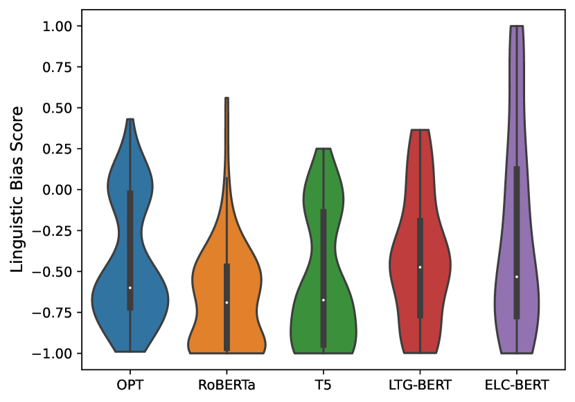
Figure 2: Violin plots of each model’s Linguistic Bias Scores (LBS) and the base model. The white dot shows the median LBS and the edge of the boxes are the 1^st and 3^rd quartiles. The width of the violins shows the density of results at that score.

GLUE.

A standard LM benchmark that tests the ability to be finetuned for general language understanding tasks. Focusing on the results in Table 2, we see that our model outperforms both the encoder baseline and the LTG-BERT model in the strict and stric-small tracks. The improvement against LTG-BERT is rather modest and could be caused by random variation. If we look at Table 9 we see that the variation is greatly affected by the WSC task – ignoring it, we get a score of $80.49^{\pm{1.44}}$ for our model and $79.52^{\pm{1.13}}$ for LTG-BERT.

MSGS.

Finally, this benchmark evaluates the preference towards linguistic explanations over spurious surface explanations. For the aggregated strict MSGS results of Table 2, the comparison appears unclear due to the large standard deviation. However, a closer inspection reveals that ELC-BERT significantly outperforms LTG-BERT by 0.16 LBS points. Figure 2 and Table 10 shows a detailed view on the score distribution.

Shared task results.

The official Dynabench results for the top-5 models for the strict and strict-small track can be found in Table 1. Looking first at the strict track results, we see that our model achieves the highest total score and BLiMP score, while we are second for GLUE and MSGS. On the strict-small track our model performs best on all benchmarks and by a substantial margin for all benchmarks.

5.2 Model variations

We compare the following modifications of the ELC-BERT architecture from Section 3:

1. Zero initialization: The layer weights are all initialized as zeros, without any bias towards the previous layer. This model also uses the residual MLP input from Equation 2. This variation is used in the strict-small track.

2. Strict normalization: This follows the previous variant with every $\bm{h}^{i}_{\text{out}}$ normalized to a unit vector.

3. Weighted output: Follows the first variant and the input to the LM head is a weighted sum of all layers. To be more concrete, we replace Equation 3 by $\bm{y}\leftarrow\operatorname{LM\_head}\!\left(\sum^{N}_{i=0}{\alpha_{i,N+1}\bm{h}^{i}_{\text{out}}}\right)$.

Model	BLiMP	Supp.	MSGS	GLUE
ELC-BERT	85.3	76.6	-0.26±0.5	78.3±3.2
+ zero initialization	84.9	78.5	-0.38±0.3	79.4±1.0
+ normalization	85.1	76.0	-0.13±0.4	78.2±3.3
+ weighted output	86.1	76.0	-0.28±0.2	78.2±0.6

Table 3: Results for the BabyLM challenge suite of evaluation datasets. We compare the performance of different variants of our model to the one submitted to the BabyLM challenge as well as the backbone model LTG-BERT on the strict dataset.

Evaluation.

Based on Table 3, we see that different variations have varying effects on the evaluation scores.

When changing the $\hat{\alpha}$ initialization to zero, we see a significant increase in performance on both the BLiMP Supplemental and the GLUE benchmarks. However, the model suffers in performance on both the BLiMP and MSGS. Overall, we see that this variation leads to better zero-shot and fine-tuning results while biasing the model more towards spurious surface features rather than linguistic features, as can be seen in Figure 3.

If we then focus on the normalization variation, we see that it underperforms in all benchmarks but one, MSGS, where it significantly performs better by 0.13 LBS points, as can be seen in more detail in Figure 3.

Finally, when looking at our weighted output variation, we see a substantial gain in performance on the BLiMP benchmark while the results on MSGS and GLUE are similar, and the results on Supplemental BLiMP slightly decrease. More detailed results on all these benchmarks can be found in Appendix D.

5.3 Layer importance

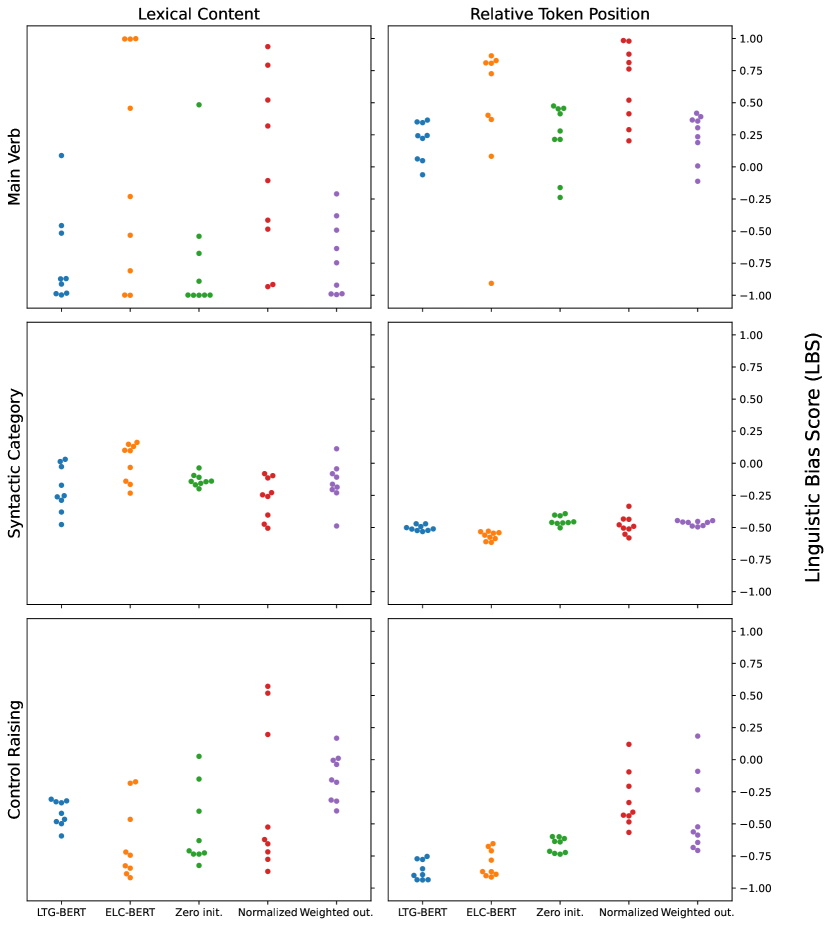
Figure 3: Detailed LBS for each model and each combination of surface and linguistic features. The Y-axis (Main Verb, Syntactic Category, and Control Raising) show the linguistic features, while the X-axis (Lexical Content, Relative Token Position) represent the surface features. Each dot represents a different fine-tuned model.

The empirical evaluation suggests that learnable layer weights are a simple but effective architectural change – but how do these learnt weights look like? In this section, we investigate the $\alpha$ values of the normalized ELC-BERT variant.

Looking at the importance matrix of ELC-BERT in Figure 1, we posit that the first 5 layers focus on surface-level information found in the embedding layer explaining its enhanced importance for the embedding layer. The next 5 layers (6-10) focus on more linguistic features by virtually ignoring the first 4 layers (0-3) and focusing primarily on the previous three layers as well as layers 4 and 5 to get some transformed information from the embedding layer. Layer 11 does much the same but focuses more on Layer 4, potentially trying to obtain some surface knowledge found in it. Finally, Layer 12 behaves similarly to Layer 11 but also puts high importance (3^rd most) on the embedding layer. This is most likely to recuperate some surface information lost in previous layers to pass to the language modelling head.

6 Conclusion

In this paper, we proposed a novel and simple modification of the transformer architecture for language modelling. We empirically tested the efficacy of our approach by participating in the BabyLM challenge – a shared task for data-efficient language modelling. Our submission ranked first on both tracks that we participated in. A more detailed evaluation shows that, when compared to a strong baseline, our approach reliably performs better on (Super)GLUE tasks. The evaluation on MSGS suggests that our approach is more likely to prefer linguistic features over spurious surface features, and the BLiMP benchmarks show comparable performance to the baseline. Finally, our proposed modification shows that the assumption that all layers are equally important is incorrect, and a more complex layer structure helps the model.

Appendix A Pre-training details

Hyperparameter	Base	Small	Small (Submitted Model)
Number of parameters	98M	24M	24M
Number of layers	12	12	12
Hidden size	768	384	384
FF intermediate size	2 048	1 024	1 024
Vocabulary size	16 384	6 144	6 144
Attention heads	12	6	6
Hidden dropout	0.1	0.1	0.1
Attention dropout	0.1	0.1	0.1
Training steps	15 625	15 625	31 250
Batch size	32 768	32 768	8 096
Initial Sequence length	128	128	128
Initial Sequence length	512	512	512
Warmup ratio	1.6%	1.6%	1.6%
Initial learning rate	0.01	0.0141	0.005
Final learning rate	0.001	0.00141	0.005
Learning rate scheduler	cosine	cosine	cosine
Weight decay	0.1	0.4	0.4
Layer norm $\epsilon$	1e-7	1e-7	1e-7
Optimizer	LAMB	LAMB	LAMB
LAMB $\epsilon$	1e-6	1e-6	1e-6
LAMB $\beta_{1}$	0.9	0.9	0.9
LAMB $\beta_{2}$	0.98	0.98	0.98
Gradient clipping	2.0	2.0	2.0

Table 4: Pre-training hyperparameters for the small-sized models (trained on strict-small) and for the base-sized models (trained on the strict track).

Appendix B Fine-tuning details

For the fine-tuning experiments, we will run multiple seeds and (for MSGS) multiple learning rates, to be able to get a more robust comparison of model performance. The detailed hyperparameters for fine-tuning can be found in Table 5.

B.0.1 GLUE

To finetune, we will use 5 different seeds: 12, 642, 369, 1267, and 2395. We will use a validation set to find our best model with early-stopping, and then test our model on a test set (here the validation set is 10% of the training sets from https://github.com/babylm/evaluation-pipeline and the test set is their validation set).

B.0.2 MSGS

To finetune, we use three different random seeds: 12, 369, and 2395, as well as three different learning rates: 1e-5, 2e-5, and 3e-5. In addition, we train for 5 epochs, with a batch size of 16 with no early stopping.

Hyperparameter	QQP, MNLI	CoLA, RTE, WSC	MSGS
	QNLI, SST-2	MRPC, MultiRC
Batch size	32	16	16
Number of epochs	10	10	5
Dropout	0.1	0.1	0.1
Warmup steps	10%	1%	6%
Peak learning rate	5e-5	7e-5	{1e-5, 2e-5, 3e-5}
Learning rate decay	cosine	cosine	linear
Weight decay	0.1	0.1	0.1
Optimizer	AdamW	AdamW	AdamW
Adam $\epsilon$	1e-8	1e-8	1e-8
Adam $\beta_{1}$	0.9	0.9	0.9
Adam $\beta_{2}$	0.999	0.999	0.999

Table 5: Hyperparameters for fine-tuning the GLUE, SuperGLUE task and MSGS tasks. We use the same hyperparameters for all ELC-BERT models, not performing any per-model hyperparameter search. The values for MSGS are adopted from (Warstadt et al., 2020b). For all models, we measure the statistics over 5 random seeds for GLUE tasks: 12, 642, 369, 1267, and 2395; and 3 seeds for MSGS tasks: 12, 369, and 2395

Appendix C BabyLM dataset

Table 6 is a detailed overview of the BabyLM dataset:

		# Words
Dataset	Domain	strict-small	strict	Proportion
CHILDES (MacWhinney, 2000)	Child-directed speech	0.44M	4.21M	5%
British National Corpus (BNC),1 dialogue portion	Dialogue	0.86M	8.16M	8%
Children’s Book Test (Hill et al., 2016)	Children’s books	0.57M	5.55M	6%
Children’s Stories Text Corpus2	Children’s books	0.34M	3.22M	3%
Standardized Project Gutenberg Corpus (Gerlach and Font-Clos, 2018)	Written English	0.99M	9.46M	10%
OpenSubtitles (Lison and Tiedemann, 2016)	Movie subtitles	3.09M	31.28M	31%
QCRI Educational Domain Corpus (QED; Abdelali et al., 2014)	Educational video subtitles	1.04M	10.24M	11%
Wikipedia3	Wikipedia (English)	0.99M	10.08M	10%
Simple Wikipedia4	Wikipedia (Simple English)	1.52M	14.66M	15%
Switchboard Dialog Act Corpus (Stolcke et al., 2000)	Dialogue	0.12M	1.18M	1%
Total	–	9.96M	98.04M	100%

Table 6: The contents of datasets for the the strict and strict-small tracks; the table is taken from Warstadt et al. (2023). ¹http://www.natcorp.ox.ac.uk   ²https://www.kaggle.com/datasets/edenbd/children-stories-text-corpus   ³https://dumps.wikimedia.org/enwiki/20221220/   ⁴https://dumps.wikimedia.org/simplewiki/20221201/

Appendix D Detailed Results

This section breaks down the aggregate scores of the benchmarks into their composing tasks. It also describes or name each task

D.1 BLiMP

The BabyLM challenge uses the BLiMP benchmark (Warstadt et al., 2020a) to evaluate the syntactic understanding of the models. Our detailed results can be found in Table 7. Its composing tasks are as follows (with descriptions taken from Warstadt et al. (2020a)):

• Anaphor Agreement (AA): the requirement that reflexive pronouns like herself (also known as anaphora) agree with their antecedents in person, number, gender, and animacy.

• Argument structure (AS): the ability of different verbs to appear with different types of arguments. For instance, different verbs can appear with a direct object, participate in the causative alternation, or take an inanimate argument.

• Binding (B): the structural relationship between a pronoun and its antecedent.

• Control/raising (CR): syntactic and semantic differences between various types of predicates that embed an infinitival VP. This includes control, raising, and tough-movement predicates.

• Determiner-noun agreement (DNA): number agreement between demonstrative determiners (e.g., this/these) and the associated noun.

• Ellipsis (E): the possibility of omitting expressions from a sentence. Because this is difficult to illustrate with sentences of equal length, our paradigms cover only special cases of noun phrase ellipsis that meet this constraint.

• Filler-gap (FG): dependencies arising from phrasal movement in, for example, wh-questions.

• Irregular forms (IF): irregular morphology on English past participles (e.g., awoken).

• Island effects (IE): restrictions on syntactic environments where the gap in a filler-gap dependency may occur.

• NPI licensing (NL): restrictions on the distribution of negative polarity items like any and ever limited to, for example, the scope of negation and only.

• Quantifiers (Q): restrictions on the distribution of quantifiers. Two such restrictions are covered: superlative quantifiers (e.g., at least) cannot be embedded under negation, and definite quantifiers and determiners cannot be subjects in existential-there constructions.

• Subject-verb agreement (SVA): subjects and present tense verbs must agree in number.

Model	AA	AS	B	CR	DNA	E	FG	IF	IE	NL	Q	SVA	Average
strict (100M words)
OPT125M	94.9	73.8	73.8	72.2	93.1	80.5	73.6	80.8	57.8	51.6	74.5	77.3	75.3
RoBERTabase	89.5	71.3	71.0	67.1	93.1	83.8	68.0	89.6	54.5	66.3	70.3	76.2	75.1
T5base	66.7	61.2	59.4	59.8	53.8	49.1	70.0	75.5	43.6	45.6	34.2	53.2	56.0
LTG-BERTbase	96.1	79.5	77.1	80.3	95.4	91.7	87.8	94.5	79.8	84.4	72.2	91.2	85.8
ELC-BERTbase	92.8	81.2	74.0	79.2	96.0	91.7	87.1	93.6	83.9	83.5	70.2	90.8	85.3
+ zero initialization	93.8	79.1	73.6	79.8	95.5	91.0	87.1	93.3	78.8	84.8	73.5	88.7	84.9
+ normalization	93.0	79.1	74.6	79.8	95.6	91.7	87.4	93.9	82.0	83.7	71.3	89.1	85.1
+ weighted output	94.7	80.7	75.7	81.3	95.7	91.6	88.9	95.9	83.2	85.7	69.2	91.1	86.1
strict-small (10M words)
OPT125M	63.8	70.6	67.1	66.5	78.5	62.0	63.8	67.5	48.6	46.7	59.6	56.9	62.6
RoBERTabase	81.5	67.1	67.3	67.9	90.8	76.4	63.5	87.4	39.9	55.9	70.5	65.4	69.5
T5base	68.9	63.8	60.4	60.9	72.2	34.4	48.2	77.6	45.6	47.8	61.2	65.0	58.8
ELC-BERTsmall	89.5	72.5	68.1	72.6	93.4	87.4	80.6	91.0	67.9	79.4	75.2	88.7	80.5

Table 7: BLiMP results for models trained both on the 100M (above the mid-horizontal line) and the 10M (below the mid-horizontal line) Baby LM dataset. The bold results represent the best model for the task. The metric used to measure is accuracy. The results are in percentage.

D.2 BLiMP Supplemental

Model	Hypernym	QA Congruence Easy	QA Congruence Tricky	Subject Aux Inversion	Turn Talking	Average
strict (100M words)
OPT125M	46.3	76.5	47.9	85.3	82.9	67.8
RoBERTabase	50.8	34.4	34.5	45.6	46.8	42.4
T5base	51.1	45.3	25.5	69.2	48.9	48.0
LTG-BERTbase	47.0	90.6	60.6	90.7	92.1	76.8
ELC-BERTbase	47.3	85.9	63.0	94.5	92.1	76.6
+ zero initialization	47.1	92.2	64.2	95.9	93.2	78.5
+ normalization	46.1	85.9	59.4	96.5	92.1	76.0
+ weighted output	48.6	87.5	57.6	96.2	90.4	76.0
strict-small (10M words)
OPT125M	50.0	54.7	31.5	80.3	57.1	54.7
RoBERTabase	49.4	31.3	32.1	71.7	53.2	47.5
T5base	48.0	40.6	21.2	64.9	45.0	43.9
ELC-BERTsmall	48.0	73.4	43.6	90.0	84.3	67.9

Table 8: BLiMP supplemental results for models trained both on the 100M (above the mid-horizontal line) and the 10M (below the mid-horizontal line) Baby LM dataset. The bold results represent the best model for the task. The metric used to measure is accuracy. The results are in percentage.

D.3 GLUE

The BabyLM challenge involves slightly modified GLUE and SuperGLUE benchmarks. It uses only a subset of the subtasks, the datasets are filtered so that they do not contain out-of-vocabulary words, and it sometimes uses non-standard metrics. Our detailed results can be found in Table 9. We list all subtasks and their metrics below:

• Boolean Questions (BoolQ; Clark et al., 2019), a yes/no Q/A dataset evaluated with accuracy.

• Corpus of Linguistic Acceptability (CoLA; Warstadt et al., 2019) evaluated with accuracy (originally evaluated with the Matthews correlation coefficient (MCC; Matthews, 1975)).

• The Multi-Genre Natural Language Inference Corpus (MNLI; Williams et al., 2018). Its development set consists of two parts: matched, sampled from the same data source as the training set, and mismatched, which is sampled from a different domain. Both parts are evaluated with accuracy.

• The Microsoft Research Paraphrase Corpus (MRPC; Dolan and Brockett, 2005), evaluated with both F₁-score (originally also evaluated with accuracy).

• Multi-Sentence Reading Comprehension (MultiRC; Khashabi et al., 2018), a multiple choice question answering dataset, evaluated with accuracy (originally evaluated with the exact match accuracy (EM) and F₁-score (over all answer options)).

• Question-answering Natural Language Inference (QNLI) constructed from the Stanford Question Answering Dataset (SQuAD; Rajpurkar et al., 2016), evaluated with accuracy.

• The Quora Question Pairs (QQP), evaluated with F₁-score (originally evaluated with accuracy).

• The Stanford Sentiment Treebank (SST-2; Socher et al., 2013), evaluated with accuracy.

• The Recognizing Textual Entailment datasets (RTE; Dagan et al., 2006; Bar-Haim et al., 2006; Giampiccolo et al., 2007; Bentivogli et al., 2009), evaluated with accuracy.

• Winograd Schema Challenge (WSC; Levesque et al., 2012) evaluated with accuracy.

Model	CoLA	SST-2	MRPC	QQP	MNLIm	MNLImm	QNLI	RTE	BoolQ	MultiRC	WSC	Average
strict (100M words)
OPT125m	74.9±0.6	87.7±0.7	81.9±0.7	84.3±0.1	75.7±0.3	77.0±0.3	82.8±0.8	58.6±2.9	66.4±0.7	61.5±0.8	52.3±12.5	73.0±3.9
RoBERTabase	75.6±0.3	88.3±0.6	84.0±0.5	85.5±0.2	77.4±0.4	78.3±0.3	83.6±0.2	50.7±1.5	67.7±0.7	64.3±0.5	61.4±0.0	74.3±0.6
T5base	76.7±0.9	89.0±0.8	85.2±1.1	86.2±0.1	77.9±0.3	78.7±0.3	84.7±0.9	55.4±2.2	67.7±1.5	65.7±0.8	61.0±1.1	75.3±1.1
LTG-BERTbase	82.7±0.8	92.0±0.4	87.4±0.7	87.9±0.1	83.0±0.4	83.4±0.5	89.1±0.5	54.7±2.4	68.4±0.5	66.0±1.4	61.4±0.0	77.9±1.1
ELC-BERTbase	82.6±0.5	91.9±1.1	89.3±0.6	88.0±0.1	83.6±0.1	83.3±0.2	89.4±0.4	60.0±2.8	70.5±1.5	66.2±2.2	56.4±9.4	78.3±3.2
+ zero initialization	82.0±0.7	92.4±0.4	88.8±1.5	88.2±0.1	84.4±0.3	84.5±0.3	90.5±0.5	63.0±1.5	72.6±1.0	65.8±1.1	61.4±0.0	79.4±1.0
+ normalization	83.1±0.4	91.9±0.4	88.6±1.3	88.0±0.1	84.1±0.2	84.3±0.2	90.5±0.4	56.2±2.4	72.0±1.5	64.9±0.6	56.9±10.2	78.2±3.3
+ weighted output	82.6±0.6	91.7±1.2	87.8±1.2	87.9±0.1	84.0±0.4	84.0±0.3	89.4±0.3	55.2±5.5	71.0±0.8	64.4±0.8	61.7±0.5	78.2±0.6
strict-small (10M words)
OPT125m	69.0±0.5	85.4±0.9	80.0±1.8	80.3±0.3	69.5±0.2	71.0±0.5	71.5±0.7	51.3±2.1	66.2±1.5	56.5±2.0	50.8±10.3	68.3±3.3
RoBERTabase	70.4±0.4	85.6±0.3	82.2±0.4	83.5±0.2	72.5±0.4	74.4±0.3	80.3±0.7	56.8±5.5	65.8±2.9	61.2±1.5	61.7±0.5	72.2±1.9
T5base	76.7±0.9	69.4±0.1	81.4±0.6	76.8±0.3	57.3±0.8	58.6±1.1	64.3±0.9	52.7±2.4	63.4±1.6	48.4±1.4	60.0±2.2	64.7±1.3
LTG-BERTsmall	77.6±0.8	88.8±0.8	82.3±0.4	85.8±0.2	78.0±0.2	78.8±0.4	85.0±0.2	53.7±4.1	64.8±2.1	64.1±0.3	60.5±1.0	74.5±1.5
ELC-BERTsmall	76.1±1.0	89.3±0.5	85.0±1.8	86.7±0.3	79.2±0.3	79.9±0.2	85.8±0.4	55.4±2.6	69.3±2.0	62.2±1.0	59.0±5.4	75.3±2.1

Table 9: A subset of GLUE results (defined by the Baby LM challenge) for both the models trained on 100M and 10M words. All the results indicate the model accuracy for the task except for MRPC and QQP where the results are based on the F1-score of the positive class. To obtain the standard deviation, each model is trained with 5 seeds, and the average accuracy/F1-score is reported. The results are reported in percentage. The bold result indicates the best model for each dataset.

D.4 MSGS

The BabyLM challenge uses a reduced set of the MSGS benchmark (Warstadt et al., 2020b) to evaluate whether the model biases linguistic features or surface features. A score of 1 means only using the linguistic features, while a score of -1 is surface features only. Table 10 shows the detailed results of the reduced MSGS benchmark. The first 5 results (MVC to RTPC) are controls, checking whether the model can recognize the feature, while the next six evaluate whether the model biases linguistic or surface features. To evaluate the performance we use the Mathews Correlation Coefficient (MCC), also called Linguistic Bias Score (LBS) for the last six tasks. The surface features in this dataset are (definitions taken from Warstadt et al. (2020b)):

• Lexical content (LC): This feature is 1 iff the sentence contains the.

• Relative token position (RTP): This feature is 1 when the precedes a, and 0 when a precedes the.

The linguistic features are (definitions taken from Warstadt et al. (2020b)):

• Main verb (MV): This feature is 1 iff the sentence’s main verb is in the -ing form.

• Control/raising (CR): This feature has value 1 iff the sentence contains the control construction.

• Syntactic category (SC): This feature is 1 iff the sentence contains an adjective.

Model	MVC	CRC	SCC	LCC	RTPC	MVLC	MVRTP	CRLC	CRRTP	SCLC	SCRTP
strict (10M words)
OPT125M	1.00±0.00	0.88±0.04	0.36±0.06	0.14±0.04	0.83±0.03	-0.55±0.12	-0.88±0.06	-0.02±0.08	-0.73±0.05	0.11±0.13	-0.59±0.04
RoBERTabase	1.00±0.00	0.75±0.12	0.57±0.22	1.00±0.00	0.92±0.07	-0.87±0.41	-0.89±0.13	-0.37±0.34	-0.54±0.13	-0.70±0.27	-0.61±0.19
T5base	1.00±0.00	0.82±0.05	0.56±0.05	1.00±0.00	0.90±0.05	-1.00±0.00	-0.95±0.03	-0.13±0.10	-0.61±0.03	0.03±0.12	-0.73±0.04
LTG-BERTbase	1.00±0.00	0.83±0.07	0.65±0.08	1.00±0.00	0.50±0.06	-0.72±0.36	0.20±0.15	-0.42±0.10	-0.86±0.08	-0.20±0.18	-0.50±0.02
ELC-BERTbase	1.00±0.00	0.89±0.10	0.76±0.07	1.00±0.00	0.77±0.11	-0.01±0.88	0.44±0.57	-0.64±0.29	-0.81±0.10	0.01±0.15	-0.57±0.03
+ zero initialization	0.94±0.17	0.94±0.02	0.52±0.14	1.00±0.00	0.97±0.03	-0.74±0.49	0.23±0.27	-0.54±0.30	-0.67±0.06	-0.13±0.05	-0.45±0.04
+ normalization	1.00±0.00	0.94±0.01	0.55±0.09	1.00±0.00	0.99±0.01	-0.03±0.71	0.65±0.30	-0.32±0.58	-0.32±0.22	-0.27±0.16	-0.48±0.07
+ weighted output	1.00±0.00	0.91±0.02	0.40±0.12	1.00±0.00	0.84±0.10	-0.71±0.29	0.24±0.18	-0.14±0.19	-0.43±0.31	-0.15±0.16	-0.47±0.02
strict-small (100M words)
OPT125M	0.97±0.01	0.58±0.06	0.76±0.06	0.55±0.12	1.00±0.00	-0.91±0.10	-0.98±0.03	-0.35±0.17	-0.73±0.05	-0.05±0.06	-0.81±0.08
RoBERTabase	0.97±0.02	0.49±0.05	0.72±0.12	0.93±0.11	0.91±0.08	-0.99±0.01	-0.94±0.04	-0.30±0.17	-0.48±0.08	-0.37±0.20	-0.93±0.10
T5base	0.28±0.04	0.25±0.06	0.72±0.03	1.00±0.00	0.87±0.03	-1.00±0.00	-0.87±0.05	-0.39±0.10	-0.44±0.07	-0.70±0.10	-0.70±0.05
LTG-BERTsmall	1.00±0.00	0.71±0.02	0.43±0.14	1.00±0.00	0.75±0.11	-0.18±0.80	0.12±0.21	-0.48±0.10	-0.58±0.04	-0.48±0.10	-0.96±0.04
ELC-BERTsmall	1.00±0.00	0.79±0.04	0.68±0.08	0.98±0.04	0.77±0.01	-0.86±0.10	0.00±0.24	-0.14±0.21	-0.57±0.02	-0.29±0.17	-0.82±0.16

Table 10: A subset of MSGS results (defined by the Baby LM challenge) for both the models trained on 100M and 10M words. All the results indicate the model MCC or LBS for the non-control tasks. To obtain the standard deviation, each model is trained with 3 seeds and 3 learning rates for the strict dataset and for ELC-BERT_small, the other strict-small datasets are trained on 5 seeds with 3 learning rates, and the average MCC/LBS is reported. The results are reported in percentage. The bold result indicates the best model for each dataset.

Appendix E Almost Stochastic Order Significance Tests

In this section, we put all the ASO significance tests between the backbone model LTG-BERT, ELC-BERT, and all its variations trained on the strict dataset for both the MSGS and GLUE benchmarks.

E.1 GLUE - strict dataset

Model	LTG-BERTbase	ELC-BERTbase	zero initialization	normalized	weighted output
LTG-BERTbase	–	1.00	1.00	1.00	1.00
ELC-BERTbase	0.69	–	1.00	1.00	1.00
+ zero initialization	0.00	0.05	–	0.00	0.00
+ normalization	0.90	1.00	1.00	–	1.00
+ weighted output	0.55	1.00	0.95	1.00	–

Table 11: The $\varepsilon_{\min}$ from the ASO significance test between each model on the GLUE dataset. Each row compares whether the model in the row is better than the one in the column. Results in bold indicate that the row model is significantly better than the one in the column.

E.2 MSGS - strict dataset

Model	LTG-BERTbase	ELC-BERTbase	zero initialization	normalized	weighted output
LTG-BERTbase	–	1.00	1.00	1.00	1.00
ELC-BERTbase	0.20	–	0.28	1.00	0.83
+ zero initialization	0.62	1.00	–	1.00	1.00
+ normalization	0.01	0.31	0.02	–	0.15
+ weighted output	0.06	1.00	0.25	1.00	–

Table 12: The $\varepsilon_{\min}$ from the ASO significance test between each model on the MSGS dataset. Each row compares whether the model in the row is better than the one in the column. Results in bold indicate that the row model is significantly better than the one in the column.

References

- Abdelali et al. (2014) Ahmed Abdelali, Francisco Guzman, Hassan Sajjad, and Stephan Vogel. 2014. The AMARA corpus: Building parallel language resources for the educational domain. In Proceedings of the Ninth International Conference on Language Resources and Evaluation (LREC’14), Reykjavik, Iceland. European Language Resources Association (ELRA).
- Bachlechner et al. (2021) Thomas Bachlechner, Bodhisattwa Prasad Majumder, Henry Mao, Gary Cottrell, and Julian McAuley. 2021. Rezero is all you need: Fast convergence at large depth. In Uncertainty in Artificial Intelligence, pages 1352–1361. PMLR.
- Bar-Haim et al. (2006) Roy Bar-Haim, Ido Dagan, Bill Dolan, Lisa Ferro, and Danilo Giampiccolo. 2006. The second pascal recognising textual entailment challenge. Proceedings of the Second PASCAL Challenges Workshop on Recognising Textual Entailment.
- Bentivogli et al. (2009) Luisa Bentivogli, Ido Dagan, Hoa Trang Dang, Danilo Giampiccolo, and Bernardo Magnini. 2009. The fifth pascal recognizing textual entailment challenge. In In Proc Text Analysis Conference (TAC’09.
- Brown et al. (2020) Tom Brown, Benjamin Mann, Nick Ryder, Melanie Subbiah, Jared D Kaplan, Prafulla Dhariwal, Arvind Neelakantan, Pranav Shyam, Girish Sastry, Amanda Askell, Sandhini Agarwal, Ariel Herbert-Voss, Gretchen Krueger, Tom Henighan, Rewon Child, Aditya Ramesh, Daniel Ziegler, Jeffrey Wu, Clemens Winter, Chris Hesse, Mark Chen, Eric Sigler, Mateusz Litwin, Scott Gray, Benjamin Chess, Jack Clark, Christopher Berner, Sam McCandlish, Alec Radford, Ilya Sutskever, and Dario Amodei. 2020. Language models are few-shot learners. In Advances in Neural Information Processing Systems, volume 33, pages 1877–1901. Curran Associates, Inc.
- Clark et al. (2019) Christopher Clark, Kenton Lee, Ming-Wei Chang, Tom Kwiatkowski, Michael Collins, and Kristina Toutanova. 2019. BoolQ: Exploring the surprising difficulty of natural yes/no questions. In Proceedings of the 2019 Conference of the North American Chapter of the Association for Computational Linguistics: Human Language Technologies, Volume 1 (Long and Short Papers), pages 2924–2936, Minneapolis, Minnesota. Association for Computational Linguistics.
- Dagan et al. (2006) Ido Dagan, Oren Glickman, and Bernardo Magnini. 2006. The pascal recognising textual entailment challenge. In Machine Learning Challenges. Evaluating Predictive Uncertainty, Visual Object Classification, and Recognising Tectual Entailment, pages 177–190, Berlin, Heidelberg. Springer Berlin Heidelberg.
- Del Barrio et al. (2018) Eustasio Del Barrio, Juan A Cuesta-Albertos, and Carlos Matrán. 2018. An optimal transportation approach for assessing almost stochastic order. In The Mathematics of the Uncertain, pages 33–44. Springer.
- Devlin et al. (2019) Jacob Devlin, Ming-Wei Chang, Kenton Lee, and Kristina Toutanova. 2019. BERT: Pre-training of deep bidirectional transformers for language understanding. In Proceedings of the 2019 Conference of the North American Chapter of the Association for Computational Linguistics: Human Language Technologies, Volume 1 (Long and Short Papers), pages 4171–4186, Minneapolis, Minnesota. Association for Computational Linguistics.
- Dolan and Brockett (2005) William B. Dolan and Chris Brockett. 2005. Automatically constructing a corpus of sentential paraphrases. In Proceedings of the Third International Workshop on Paraphrasing (IWP2005).
- Dror et al. (2019) Rotem Dror, Segev Shlomov, and Roi Reichart. 2019. Deep dominance - how to properly compare deep neural models. In Proceedings of the 57th Annual Meeting of the Association for Computational Linguistics, pages 2773–2785, Florence, Italy. Association for Computational Linguistics.
- Gao et al. (2021) Leo Gao, Jonathan Tow, Stella Biderman, Sid Black, Anthony DiPofi, Charles Foster, Laurence Golding, Jeffrey Hsu, Kyle McDonell, Niklas Muennighoff, Jason Phang, Laria Reynolds, Eric Tang, Anish Thite, Ben Wang, Kevin Wang, and Andy Zou. 2021. A framework for few-shot language model evaluation.
- Gerlach and Font-Clos (2018) Martin Gerlach and Francesc Font-Clos. 2018. A standardized Project Gutenberg corpus for statistical analysis of natural language and quantitative linguistics. Computing Research Repository, arXiv:1812.08092.
- Giampiccolo et al. (2007) Danilo Giampiccolo, Bernardo Magnini, Ido Dagan, and Bill Dolan. 2007. The third PASCAL recognizing textual entailment challenge. In Proceedings of the ACL-PASCAL Workshop on Textual Entailment and Paraphrasing, pages 1–9, Prague. Association for Computational Linguistics.
- He et al. (2016) Kaiming He, Xiangyu Zhang, Shaoqing Ren, and Jian Sun. 2016. Deep Residual Learning for Image Recognition. In Proceedings of 2016 IEEE Conference on Computer Vision and Pattern Recognition, CVPR ’16, pages 770–778. IEEE.
- Hill et al. (2016) Felix Hill, Antoine Bordes, Sumit Chopra, and Jason Weston. 2016. The Goldilocks principle: Reading children’s books with explicit memory representations.
- Howard and Ruder (2018) Jeremy Howard and Sebastian Ruder. 2018. Universal language model fine-tuning for text classification. In Proceedings of the 56th Annual Meeting of the Association for Computational Linguistics (Volume 1: Long Papers), pages 328–339, Melbourne, Australia. Association for Computational Linguistics.
- Jawahar et al. (2019) Ganesh Jawahar, Benoît Sagot, and Djamé Seddah. 2019. What does BERT learn about the structure of language? In Proceedings of the 57th Annual Meeting of the Association for Computational Linguistics, pages 3651–3657, Florence, Italy. Association for Computational Linguistics.
- Joshi et al. (2020) Pratik Joshi, Sebastin Santy, Amar Budhiraja, Kalika Bali, and Monojit Choudhury. 2020. The state and fate of linguistic diversity and inclusion in the NLP world. In Proceedings of the 58th Annual Meeting of the Association for Computational Linguistics, pages 6282–6293, Online. Association for Computational Linguistics.
- Khashabi et al. (2018) Daniel Khashabi, Snigdha Chaturvedi, Michael Roth, Shyam Upadhyay, and Dan Roth. 2018. Looking beyond the surface: A challenge set for reading comprehension over multiple sentences. In Proceedings of the 2018 Conference of the North American Chapter of the Association for Computational Linguistics: Human Language Technologies, Volume 1 (Long Papers), pages 252–262, New Orleans, Louisiana. Association for Computational Linguistics.
- Kondratyuk and Straka (2019) Dan Kondratyuk and Milan Straka. 2019. 75 languages, 1 model: Parsing Universal Dependencies universally. In Proceedings of the 2019 Conference on Empirical Methods in Natural Language Processing and the 9th International Joint Conference on Natural Language Processing (EMNLP-IJCNLP), pages 2779–2795, Hong Kong, China. Association for Computational Linguistics.
- Levesque et al. (2012) Hector J. Levesque, Ernest Davis, and Leora Morgenstern. 2012. The winograd schema challenge. In Proceedings of the Thirteenth International Conference on Principles of Knowledge Representation and Reasoning, KR’12, page 552–561. AAAI Press.
- Lison and Tiedemann (2016) Pierre Lison and Jörg Tiedemann. 2016. OpenSubtitles2016: Extracting large parallel corpora from movie and TV subtitles. In Proceedings of the Tenth International Conference on Language Resources and Evaluation (LREC’16), pages 923–929, Portorož, Slovenia. European Language Resources Association (ELRA).
- MacWhinney (2000) Brian MacWhinney. 2000. The CHILDES project: The database, volume 2. Psychology Press.
- Matthews (1975) B.W. Matthews. 1975. Comparison of the predicted and observed secondary structure of t4 phage lysozyme. Biochimica et Biophysica Acta (BBA) - Protein Structure, 405(2):442–451.
- Niu et al. (2022) Jingcheng Niu, Wenjie Lu, and Gerald Penn. 2022. Does BERT rediscover a classical NLP pipeline? In Proceedings of the 29th International Conference on Computational Linguistics, pages 3143–3153, Gyeongju, Republic of Korea. International Committee on Computational Linguistics.
- Raffel et al. (2020) Colin Raffel, Noam Shazeer, Adam Roberts, Katherine Lee, Sharan Narang, Michael Matena, Yanqi Zhou, Wei Li, and Peter J. Liu. 2020. Exploring the limits of transfer learning with a unified text-to-text transformer. Journal of Machine Learning Research, 21(140):1–67.
- Rajpurkar et al. (2016) Pranav Rajpurkar, Jian Zhang, Konstantin Lopyrev, and Percy Liang. 2016. SQuAD: 100,000+ questions for machine comprehension of text. In Proceedings of the 2016 Conference on Empirical Methods in Natural Language Processing, pages 2383–2392, Austin, Texas. Association for Computational Linguistics.
- Samuel (2023) David Samuel. 2023. Mean berts make erratic language teachers: the effectiveness of latent bootstrapping in low-resource settings.
- Samuel et al. (2023) David Samuel, Andrey Kutuzov, Lilja Øvrelid, and Erik Velldal. 2023. Trained on 100 million words and still in shape: BERT meets British National Corpus. In Findings of the Association for Computational Linguistics: EACL 2023, pages 1954–1974, Dubrovnik, Croatia. Association for Computational Linguistics.
- Socher et al. (2013) Richard Socher, Alex Perelygin, Jean Wu, Jason Chuang, Christopher D. Manning, Andrew Ng, and Christopher Potts. 2013. Recursive deep models for semantic compositionality over a sentiment treebank. In Proceedings of the 2013 Conference on Empirical Methods in Natural Language Processing, pages 1631–1642, Seattle, Washington, USA. Association for Computational Linguistics.
- Srivastava et al. (2015) Rupesh K Srivastava, Klaus Greff, and Jürgen Schmidhuber. 2015. Training very deep networks. In Advances in Neural Information Processing Systems, volume 28. Curran Associates, Inc.
- Stolcke et al. (2000) Andreas Stolcke, Klaus Ries, Noah Coccaro, Elizabeth Shriberg, Rebecca Bates, Daniel Jurafsky, Paul Taylor, Rachel Martin, Marie Meteer, and Carol Van Ess-Dykema. 2000. Dialogue act modeling for automatic tagging and recognition of conversational speech. Computational Linguistics, 26(3):339–371.
- Strubell et al. (2019) Emma Strubell, Ananya Ganesh, and Andrew McCallum. 2019. Energy and policy considerations for deep learning in NLP. In Proceedings of the 57th Annual Meeting of the Association for Computational Linguistics, pages 3645–3650, Florence, Italy. Association for Computational Linguistics.
- Tenney et al. (2019) Ian Tenney, Dipanjan Das, and Ellie Pavlick. 2019. BERT rediscovers the classical NLP pipeline. In Proceedings of the 57th Annual Meeting of the Association for Computational Linguistics, pages 4593–4601, Florence, Italy. Association for Computational Linguistics.
- Thompson et al. (2020) Neil C. Thompson, Kristjan Greenewald, Keeheon Lee, and Gabriel F. Manso. 2020. The computational limits of deep learning.
- Ulmer et al. (2022) Dennis Ulmer, Christian Hardmeier, and Jes Frellsen. 2022. deep-significance: Easy and meaningful signifcance testing in the age of neural networks. In ML Evaluation Standards Workshop at the Tenth International Conference on Learning Representations.
- Vaswani et al. (2017) Ashish Vaswani, Noam Shazeer, Niki Parmar, Jakob Uszkoreit, Llion Jones, Aidan N Gomez, Łukasz Kaiser, and Illia Polosukhin. 2017. Attention is all you need. Advances in neural information processing systems, 30.
- Wang et al. (2019) Alex Wang, Yada Pruksachatkun, Nikita Nangia, Amanpreet Singh, Julian Michael, Felix Hill, Omer Levy, and Samuel Bowman. 2019. Superglue: A stickier benchmark for general-purpose language understanding systems. In Advances in Neural Information Processing Systems, volume 32. Curran Associates, Inc.
- Wang et al. (2018) Alex Wang, Amanpreet Singh, Julian Michael, Felix Hill, Omer Levy, and Samuel Bowman. 2018. GLUE: A multi-task benchmark and analysis platform for natural language understanding. In Proceedings of the 2018 EMNLP Workshop BlackboxNLP: Analyzing and Interpreting Neural Networks for NLP, pages 353–355, Brussels, Belgium. Association for Computational Linguistics.
- Warstadt et al. (2023) Alex Warstadt, Aaron Mueller, Leshem Choshen, Ethan Gotlieb Wilcox, Chengxu Zhuang, Juan Ciro, Rafael Mosquera, Adina Williams, Bhargavi Paranjabe, Tal Linzen, and Ryan Cotterell. 2023. Findings of the 2023 BabyLM Challenge: Sample-efficient pretraining on developmentally plausible corpora. In Proceedings of the 2023 BabyLM Challenge. Association for Computational Linguistics (ACL).
- Warstadt et al. (2020a) Alex Warstadt, Alicia Parrish, Haokun Liu, Anhad Mohananey, Wei Peng, Sheng-Fu Wang, and Samuel R Bowman. 2020a. Blimp: The benchmark of linguistic minimal pairs for english. Transactions of the Association for Computational Linguistics, 8:377–392.
- Warstadt et al. (2019) Alex Warstadt, Amanpreet Singh, and Samuel R. Bowman. 2019. Neural network acceptability judgments. Transactions of the Association for Computational Linguistics, 7:625–641.
- Warstadt et al. (2020b) Alex Warstadt, Yian Zhang, Haau-Sing Li, Haokun Liu, and Samuel R Bowman. 2020b. Learning which features matter: Roberta acquires a preference for linguistic generalizations (eventually). arXiv preprint arXiv:2010.05358.
- Williams et al. (2018) Adina Williams, Nikita Nangia, and Samuel Bowman. 2018. A broad-coverage challenge corpus for sentence understanding through inference. In Proceedings of the 2018 Conference of the North American Chapter of the Association for Computational Linguistics: Human Language Technologies, Volume 1 (Long Papers), pages 1112–1122, New Orleans, Louisiana. Association for Computational Linguistics.