Rolling spheres and the Willmore energy

Zusammenfassung

The Willmore energy plays a central role in the conformal geometry of surfaces in the conformal 3-sphere $S^{3}$. It also arises as the leading term in variational problems ranging from black holes, to elasticity, and cell biology. In the computational setting a discrete version of the Willmore energy is desired. Ideally it should have the same symmetries as the smooth formulation. Such a Möbius invariant discrete Willmore energy for simplicial surfaces was introduced by Bobenko.

In the present paper we provide a new geometric interpretation of the discrete energy as the curvature of a rolling spheres connection in analogy to the smooth setting where the curvature of a connection induced by the mean curvature sphere congruence gives the Willmore integrand. We also show that the use of a particular projective quaternionic representation of all relevant quantities gives clear geometric interpretations which are manifestly Möbius invariant.

KnöppelBerlin PinkallBerlin SchröderPasadena SolimanPasadena Mathematics, Technische Universität Berlin, Straße des 17. Juni 135, 10623 Berlin, Germanyknoeppel@math.tu-berlin.de Mathematics, Technische Universität Berlin, Straße des 17. Juni 135, 10623 Berlin, Germanypinkall@math.tu-berlin.de Computing + Mathematical Sciences, California Institute of Technology, 1200 E California Blvd, Pasadena, California 91125, United States of Americaps@caltech.edu Computing + Mathematical Sciences, California Institute of Technology, 1200 E California Blvd, Pasadena, California 91125, United States of Americaysoliman@caltech.edu MnLargeSymbols’164 MnLargeSymbols’171

1 Introduction

The Willmore energy is the most well-studied example of a surface functional that is invariant under Möbius transformations. For an immersion $f:M\to\mathbb{R}^{3}$ of a smooth two-dimensional manifold, the Willmore energy is defined as

(1) $$\mathcal{W}=\int_{M}(H^{2}-K)\,\sigma_{f}.$$

Here $H=\tfrac{1}{2}(\kappa_{1}+\kappa_{2})$ is the mean curvature, $K=\kappa_{1}\kappa_{2}$ the Gaussian curvature, $\sigma_{f}$ the induced volume form, and $\kappa_{1}$ and $\kappa_{2}$ are the principal curvatures of the immersion, resulting in a Möbius invariant integrand. Recall that the group of Möbius transformations of $S^{3}$ consists of the diffeomorphisms of $S^{3}$ carrying round 2-spheres into round 2-spheres. By adding a point at $\infty$ we can consider $\mathbb{R}^{3}$ as a conformal submanifold of the one-point compactification $S^{3}=\mathbb{R}^{3}\cup\{\infty\}$ and treat Möbius transformations as conformal diffeomorphisms of $\mathbb{R}^{3}\cup\{\infty\}$. The group of Möbius transformations of $\mathbb{R}^{3}$ fixing $\infty$ is generated by the orthogonal transformations (isometries fixing the origin), homeotheties ($p\in\mathbb{R}^{3}\mapsto\lambda p$, $\lambda>0$), and translations. Also appending inversion in the unit sphere to this list, the set of transformations generates the full group of Möbius transformations of $S^{3}$.

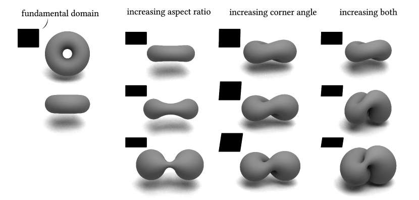
Abbildung 1: The discrete formulation of the Willmore energy enables the computation of (constrained) critical points via numerical minimization. The discrete constrained Willmore tori visualized here provide realizations of points in Teichmüller space as discrete surfaces in $S^{3}$.

In the smooth setting the Willmore energy, due to its invariance under Möbius transformation of $S^{3}$, plays a central role in conformal geometry and has stimulated many interesting research directions [22, 6, 26]. In 2012, Marques and Neves used the Almgren-Pitts min-max theory to resolve the celebrated Willmore conjecture stating that, up to Möbius transformation, the Clifford torus minimizes the Willmore energy among immersed tori in $\mathbb{R}^{3}$ [24]. The Willmore energy also arises in a variety of scientific domains. In cell biology, it models the geometry and locomotion of lipid bilayers [23, 10, 16, 12, 11]. In general relativity, it appears as the leading term of the Hawking mass [15, 20]. In nonlinear elasticity, it measures the bending energy of thin plates [13]. The Willmore energy is also popular in computational geometry and computer graphics due to the regularizing effects of its gradient flow [5, 30, 28, 27]. Constrained Willmore surfaces also appear in a theory that encapsulates minimal surfaces, CMC surfaces, and Willmore surfaces [26]—see Figure 1 for numerical examples of constrained Willmore tori computed following the approach in [30]. As the importance of the Willmore energy is evidenced in the context of differential geometry and physics, it is desirable to have a rich theory of discrete Willmore surfaces.

Discrete Setup

We study the discrete differential geometry of the Möbius invariant discretization of the Willmore energy on a simplicial surface $\mathsf{M}=(\mathsf{V},\mathsf{E},\mathsf{F})$ [3, 5], where $\mathsf{V}$ denotes the set of vertices $i$, $\mathsf{E}$ the set of oriented edges $i\mkern-1.0muj$, and $\mathsf{F}$ the set of oriented triangles $ijk$. An immersion into $S^{3}$ is given by vertex positions $\mathtt{f}_{i}\in S^{3}$ for $i\in\mathsf{V}$. The discrete energy $\mathcal{W}$ then is defined in terms of the intersection angles $\beta_{i\mkern-1.0muj}$ between the circumcircles $\mathtt{C}_{ijk}$ and $\mathtt{C}_{jil}$ of adjacent faces $ijk$ and $jil$ and using the negative angle defect to measure the planarity of each vertex star after sending $\mathtt{f}_{i}$ to infinity with a Möbius transformation:

(2) $$\mathcal{W}\coloneqq\tfrac{1}{2}\sum_{i\in\mathsf{V}}\mathcal{W}_{i},\qquad\mathcal{W}_{i}:=\sum_{i\mkern-1.0muj}\beta_{i\mkern-1.0muj}-2\pi.$$

Since the discrete energy is defined using only the angles between circles it is Möbius invariant. Furthermore, it is non-negative and $\mathcal{W}_{i}+K_{i}\geq 0$ where $K_{i}$ is the usual discrete Gaussian curvature (angle defect). Finally it vanishes when the vertex star is convex and $\mathtt{f}_{i}$ and all its neighbors lie on a common sphere. These properties of $\mathcal{W}_{i}$ mirror the smooth setting in that $(H^{2}-K)\,\sigma_{f}$ is non-negative, Möbius invariant, and measures infinitesimal sphericality ($\kappa_{1}=\kappa_{2}$). Together, these properties justify calling it the discrete Willmore energy. Recently, $\Gamma$-convergence of the functional has been established with respect to weak-$*$ convergence in $W^{1,\infty}$ as graphs of the piecewise linear surface to the smooth surface [14]. Consistency of the local approximation of the energy is also known for triangulations aligned to principal curvature directions [4].

Rolling Mean Curvature Spheres: Smooth and Discrete

To express the Willmore energy in a manifestly Möbius invariant way, one introduces the conformal Gauss map, also known as the mean curvature sphere congruence:

(3) $$S:M\to\mathcal{S}{}\subset\mathbb{R}^{4,1},\qquad\text{satisfying }T_{f(p)}S_{p}=df(T_{p}M)\text{ and }H_{S_{p}}=H_{p},$$

where $\mathcal{S}{}$ is the Lorentzian space of 2-spheres in $S^{3}$ (see Section 2.2), $p\in M$, $H_{S_{p}}$ the mean curvature of the sphere $S_{p}$, and $H_{p}$ the mean curvature of the immersion $f$ at $p$ [2, 7, 9]. The conformal Gauss map is Möbius invariant, even though the mean curvature itself is not. A classical result due to Blaschke is that the Willmore energy is equal to the area of the conformal Gauss map [2]. A modern treatment of conformal submanifold geometry using the machinery of Cartan geometries was given in [29, 9], and Sharpe showed that the Willmore energy can be realized as the curvature of a Cartan geometry obtained by restricting the flat Möbius structure of $S^{3}$ to an immersed surface [29].

To elucidate the differential geometric interpretation of the discrete energy, we first develop a related geometric interpretation of the Willmore energy in the smooth setting. The main idea is that the Willmore integrand can be realized as the curvature of a rolling spheres connection in the same way as the Gauss curvature form can be realized as the curvature of the Levi-Civita connection—geometrically, the Levi-Civita connection describes how to roll tangent planes over the surface without slipping or twisting. Extrinsically, the process of rolling tangent planes is characterized by the trajectories of the induced parallel transport being orthogonal to the tangent planes themselves. By following the parallel transport around a closed loop one obtains an affine map of the tangent plane onto itself. The curvature of the connection at a point $p$ is the affine map of $T_{p}M$ onto itself obtained as the limit of following the parallel transport around infinitesimal loops based at $p$. As the Levi-Civita connection is torsion free, the curvature fixes the point $p$ and on the tangent space $df(T_{p}M)$ acts by a rotation around the normal with an angle given by the Gauss curvature of the surface.

To obtain a Möbius geometric generalization, we replace the tangent plane congruence with an arbitrary tangent sphere congruence and replace the Levi-Civita connection with a Möbius connection whose parallel transport trajectories are orthogonal to the sphere congruence. This orthogonal trajectories property, visualized in Figure 2, justifies calling the connection a rolling spheres connection since the trajectories follow the paths that one would get by rolling a sphere over the surface in Möbius three-space. In the special case when the sphere congruence is given by the Möbius invariant mean curvature sphere congruence, we find that the Willmore energy arises as the rotational component of the curvature form of the connection obtained by rolling the mean curvature spheres over the surface. Our main result about the discrete energy provides an analogous geometric interpretation of it: we prove that the discrete Willmore energy can be computed from the curvature of a Möbius connection obtained by rolling the circumspheres from one edge to the next around a vertex.

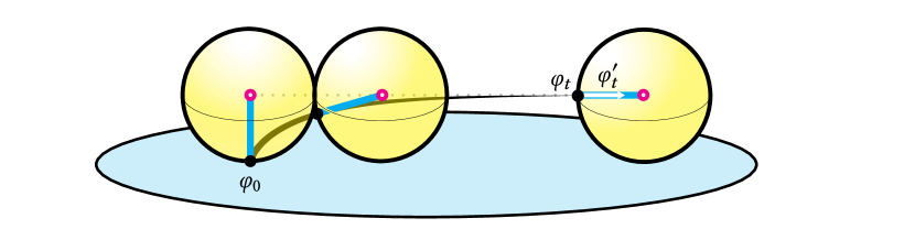
Abbildung 2: Möbius geometric rolling of a sphere congruence traces out trajectories that intersect the spheres orthogonally. The tractrix curve visualized above is obtained by rolling a sphere of constant radius over a flat plane.

Quaternionic Projective Geometry and $S^{3}$

In Section 2 we review the basics of the quaternionic projective (i.e., Möbius) geometry of $S^{4}$ as presented in [8] and specialize the situation to $S^{3}$ by restricting the group of quaternionic projective transformations of $S^{4}$ to those which preserve a fixed Möbius 3-sphere, $S^{3}$, in $S^{4}$. We then realize spaces of geometric objects associated to this quaternionic projective geometry (e.g., the spaces of oriented 2-spheres, circles, and point pairs in $S^{3}$) as spaces of quaternionic matrices. We define an algebraic structure, resembling vector calculus in $\mathbb{R}^{3}$, on the space of $p$-spheres in $S^{3}$ for $p\in\{0,1,2\}$. The vector calculus of $p$-spheres involves a cross product and a dot product that act on the algebraic representations of oriented $p$-spheres in $S^{3}$. The cross-product of two intersecting circles, for example, produces the sine of their intersection angle multiplying the unique circle orthogonal to both circles. On the other hand, their dot product produces the cosine of the intersection angle. In Section 3 we use this quaternionic formalism to describe the geometry of rolling spheres in both the smooth and discrete settings using quaternionic connections. The quaternionic formalism we present here should be of independent geometric interest—our experience is that it is geometrically meaningful as well as quite efficient and easily implemented on a computer for the algorithmic manipulation of spheres and circles.

Recently, there have been a several authors who have studied fundamental properties of quaternionic Möbius transformations. Fixed points and conjugacy classes of Möbius transformations of $S^{3}$ have been characterized in [18, 1]. Quaternionic holomorphic geometry provides an elegant description of surfaces in 3-space and 4-space that has been especially fruitful in the study of Willmore surfaces [17, 8]. In this context the quaternionic realization of the space of oriented 2-spheres plays a central role.

2 Möbius Geometry of $S^{3}$ with Quaternions

It is natural to study the discrete Willmore energy in the Möbius geometry of $S^{3}$ for which we will employ a quaternionic projective model. We begin with a review of the quaternionic projective geometry of $\mathbb{H}\mathsf{P}^{1}$ and by restricting the group of Möbius transformations to those fixing a three-sphere $S^{3}$ inside of $S^{4}$ we obtain a quaternionic projective model of the Möbius geometry of $S^{3}$.

2.1 Möbius transformations preserving $S^{3}$

The quaternionic projective model of $S^{4}$ is based on the observation that $\mathbb{H}\mathsf{P}^{1}$ is conformally equivalent to $S^{4}$ [8, Section 3.1]. The group $\mathrm{GL}(2;\mathbb{H})$ acts on $\mathbb{H}\mathsf{P}^{1}$ by $\mathsf{A}(\psi\mathbb{H})=(\mathsf{A}\psi)\mathbb{H}$, $\mathsf{A}\in\mathrm{GL}(2;\mathbb{H})$, and acts by Möbius transformations on $S^{4}$. Moreover, all orientation preserving conformal differeomorphisms are realized this way and the representation of a Möbius transformation is unique up to a real scale [21].

A three-sphere inside of $S^{4}$ is determined by the isotropic lines of an indefinite Hermitian inner product on $\mathbb{H}^{2}$ [8, Chapter 10]. We fix the indefinite Hermitian inner product

(4) $$\langle\begin{pmatrix}\psi_{0}\\ \psi_{1}\end{pmatrix},\begin{pmatrix}\varphi_{0}\\ \varphi_{1}\end{pmatrix}\rangle=\bar{\psi}_{0}\varphi_{1}+\bar{\psi}_{1}\varphi_{0}.$$

The isotropic lines form a conformal model of $S^{3}$:

(5) $$S^{3} \coloneqq\big{\{}\psi\mathbb{H}\in\mathbb{H}\mathsf{P}^{1}\,\,\mid\,\,\langle\psi,\psi\rangle=0\big{\}}$$

(6) $$=\Big{\{}\begin{pmatrix}p\\ 1\end{pmatrix}\mathbb{H}\,\,\mid\,\,p\in\mathbb{R}^{3}\cong\operatorname{Im}\mathbb{H}\Big{\}}\cup\Big{\{}\infty\Big{\}}.$$

A unitary transformation $\mathsf{A}$ is an automorphism of $(\mathbb{H}^{2},\langle\cdot,\,\cdot\rangle)$, i.e. an invertible linear map $\mathsf{A}\in\mathrm{GL}(2;\mathbb{H})$ satisfying $\langle\mathsf{A}\psi,\mathsf{A}\varphi\rangle=\langle\psi,\varphi\rangle$ for all $\psi,\varphi\in\mathbb{H}^{2}$, and we denote the group of all such transformations as $\mathrm{Sp}(1,1)$. They satisfy $\mathsf{A}^{*}\mathsf{A}=\mathsf{I}$ where $\mathsf{I}$ is the identity matrix and $\mathsf{A}^{*}$ the adjoint with respect to the indefinite Hermitian form

(7) $$\mathsf{A}^{*}=\begin{pmatrix}\bar{d}&\bar{b}\\ \bar{c}&\bar{a}\end{pmatrix}\quad\text{for}\quad\mathsf{A}=\begin{pmatrix}a&b\\ c&d\end{pmatrix}.$$

Evidently the action of $\mathrm{Sp}(1,1)$ preserves $S^{3}$ and since the restriction of a conformal map of $S^{4}$ to $S^{3}$ is still conformal, we deduce that elements of $\mathrm{Sp}(1,1)$ can be identified with orientation preserving Möbius transformations of $S^{3}$.

These transformations can be written in terms of simpler, geometrically meaningful components associated with the generators of the group of Möbius transformations (see Appendix A for a proof).

Proposition 2.1.

Let $\mathsf{A}\in\mathrm{Sp}(1,1)$. Then there exists unique $x,y\in\mathbb{R}^{3}$ and $\mu\in\mathbb{H}$ satisfying

(8) $$\mathsf{A}=\begin{pmatrix}1&0\\ y&1\end{pmatrix}\begin{pmatrix}\mu&0\\ 0&\bar{\mu}^{-1}\end{pmatrix}\begin{pmatrix}1&x\\ 0&1\end{pmatrix}.$$

The factors have straightforward geometric interpretations. For $x\in\mathbb{R}^{3}$ the matrix

(9) $$\mathsf{T}_{x}\coloneqq\begin{pmatrix}1&x\\ 0&1\end{pmatrix},\qquad\mathsf{T}_{x}\begin{pmatrix}p\\ 1\end{pmatrix}\mathbb{H}=\begin{pmatrix}p+x\\ 1\end{pmatrix}\mathbb{H}$$

describes the translation by $x$. For $\mu\in\mathbb{H}$ the matrix

(10) $$\mathsf{R}_{\mu}\coloneqq\begin{pmatrix}\mu&0\\ 0&\bar{\mu}^{-1}\end{pmatrix},\qquad\mathsf{R}_{\mu}\begin{pmatrix}p\\ 1\end{pmatrix}\mathbb{H}=\begin{pmatrix}\mu\,p\,\bar{\mu}\\ 1\end{pmatrix}\mathbb{H}$$

describes the stretch rotation given by conjugation with $\mu$. Lastly, for $y\in\mathbb{R}^{3}$ the matrix

(11) $$\hat{\mathsf{T}}_{y}\coloneqq\begin{pmatrix}1&0\\ y&1\end{pmatrix},\qquad\hat{\mathsf{T}}_{y}\begin{pmatrix}p\\ 1\end{pmatrix}\mathbb{H}=\begin{pmatrix}(p^{-1}+y)^{-1}\\ 1\end{pmatrix}\mathbb{H}$$

describes the inversion in the unit sphere, composed with a translation by $-y$, followed by another inversion in the unit sphere. Analogous to how a translation shifts the origin, the transformation $\hat{\mathsf{T}}_{y}$ shifts the infinity point.

Remark 2.2.

Each of the terms, $\hat{\mathsf{T}}_{y}$, $\mathsf{R}_{\mu}$, $\mathsf{T}_{x}$, in Proposition 8 describes an orientation preserving Möbius transformations of $S^{3}$, hence the group $\mathrm{Sp}(1,1)$ contains only orientation preserving Möbius transformations of $S^{3}$. Specifically, inversion in a 2-sphere is not an orientation preserving Möbius transformation and thus not representable by an element of $\mathrm{Sp}(1,1)$.

To obtain all Möbius transformations of $S^{3}$ one needs to consider the larger group

(12) $${\operatorname{M\ddot{o}b}}(3)\coloneqq\Big{\{}\mathsf{A}\in\mathbb{H}^{2\times 2}\leavevmode\nobreak\ \mid\leavevmode\nobreak\ \mathsf{A}^{*}\mathsf{A}=\pm\mathsf{I}\Big{\}}.$$

The orientation reversing Möbius transformations of $S^{3}$ are those elements satisfying $\mathsf{A}^{*}\mathsf{A}=-\mathsf{I}$.

Remark 2.3.

Both $\mathrm{Sp}(1,1)$ and ${\operatorname{M\ddot{o}b}}(3)$ are double covers of the group of orientation preserving and all Möbius transformations of $S^{3}$, respectively, and so one should consider the quotients of these groups by the order two subgroup $\{+\mathsf{I},-\mathsf{I}\}$ if working with the double cover directly is not desired.

The group ${\operatorname{M\ddot{o}b}}(3)$ has two connected components with $\mathrm{Sp}(1,1)$ being path connected to the identity. Therefore, the Lie algebra of ${\operatorname{M\ddot{o}b}}(3)$ is equal to the Lie algebra of $\mathrm{Sp}(1,1)$ denoted

(13) $$\mathfrak{sp}(1,\mkern-1.0mu1)=\big{\{}\mathsf{Y}\in\mathbb{H}^{2\times 2}\,\,\mid\,\,\mathsf{Y}^{*}+\mathsf{Y}=0\big{\}}.$$

Elements of the Lie algebra $\mathsf{Y}\in\mathfrak{sp}(1,\mkern-1.0mu1)$ can be integrated into a 1-parameter family of Möbius transformations

(14) $$t\mapsto\exp(t\mathsf{Y})$$

using the exponential map

(15) $$\exp:\mathfrak{sp}(1,\mkern-1.0mu1)\to\mathrm{Sp}(1,1)\qquad\exp\mathsf{A}\coloneqq\sum_{n=0}^{\infty}\frac{\mathsf{A}^{n}}{n!}.$$

Elements of the Lie algebra describe infinitesimal Möbius transformations of $S^{3}$. The vector field associated with $\mathsf{Y}\in\mathfrak{sp}(1,\mkern-1.0mu1)$ is given by

(16) $$\mathsf{V}_{\mathsf{Y}}(\mathsf{p})=\left.\frac{d}{dt}\right|_{t=0}\exp(t\mathsf{Y})\cdot\mathsf{p}.$$

In this way $\mathfrak{sp}(1,\mkern-1.0mu1)$ is identified with the algebra of Möbius vector fields of $S^{3}$.

Two important operations on matrices are the inner product on $\mathbb{H}^{2\times 2}$:

(17) $$\langle\mathsf{A},\mathsf{B}\rangle=-\tfrac{1}{2}\operatorname{tr}_{\mathbb{R}}(\mathsf{AB}).$$

and the cross product on $\mathbb{H}^{2\times 2}$ defined via the commutator:

(18) $$\mathsf{A}\times\mathsf{B}\coloneqq\tfrac{1}{2}[\mathsf{A},\mathsf{B}]=\tfrac{1}{2}(\mathsf{AB}-\mathsf{BA}),$$

for $\mathsf{A},\mathsf{B}\in\mathbb{H}^{2\times 2}$. Conveniently, the product of two matrices $\mathsf{A},\mathsf{B}\in\mathbb{H}^{2\times 2}$ can be written as one half the sum of the commutator and anti-commutator:

(19) $$\mathsf{A}\mathsf{B}=\tfrac{1}{2}\{\mathsf{A},\mathsf{B}\}+\mathsf{A}\times\mathsf{B}.$$

For matrices describing inversions in spheres half the anti-commutator equals minus the inner product (see Remark 2.5).

Abbildung 3: Conjugating a matrix $\mathsf{B}$ by a Möbius transformation $\mathsf{A}$ corresponds to transforming the inputs and outputs of the Möbius transformation described by $\mathsf{B}$ into new coordinates determined by $\mathsf{A}$.

To conclude this section, we note that when transforming the coordinates by a Möbius transformation $\mathsf{A}\in{\operatorname{M\ddot{o}b}}(3)$ the action of another Möbius transformation $\mathsf{B}\in{\operatorname{M\ddot{o}b}}(3)$ must be conjugated by $\mathsf{A}$ to describe the same Möbius transformation in the new coordinates:

(20) $$\tilde{\mathsf{B}}=\mathsf{A}\,\mathsf{B}\,\mathsf{A}^{-1}.$$

See Figure 3 for an illustration of the action of conjugation by a Möbius transformation. This relationship is of great practical importance. Any argument involving Möbius invariant quantities can be answered assuming a convenient Möbius transformation. For example, the angle between two intersecting spheres is the dihedral angle between the two planes that result from sending a point common to both spheres to infinity.

2.2 Spaces of Spheres in $S^{3}$

In this section we describe how to realize the space of oriented $p$-spheres for $p\in\{0,1,2\}$ inside of $\mathbb{H}^{2\times 2}$ in a geometric way by associating Möbius transformations with each $p$-sphere in $S^{3}$. These constructions are motivated by the natural association of $p$-spheres associated with cells of a simplicial surface: a circumsphere for each unoriented edge, a circumcircle for each face, and a point pair for each oriented edge. In Section 2.5 we use the algebraic structure on $\mathbb{H}^{2\times 2}$ to manipulate these $p$-spheres algebraically in a geometrically intuitive way.

To wit, each oriented 2-sphere is associated with the Möbius transformation of inversion in that sphere yielding the “space of spheres” inside $\mathbb{H}^{2\times 2}$. With each oriented circle in $S^{3}$ we define the inversion in the circle as the Möbius transformation that when restricted to any 2-sphere containing the circle is an inversion in the circle in $S^{2}$. It can also be computed by composing the inversions in spheres orthogonally intersecting in the circle. Describing this circle inversion as an element of $\mathbb{H}^{2\times 2}$ realizes the “space of circles” inside of $\mathbb{H}^{2\times 2}$. Finally, the inversion in an oriented point pair is the Möbius transformation that when restricted to any circle containing the pair of points is the inversion in a pair of points in $S^{1}$. It is equal to the Euclidean inversion $x\mapsto-x$ after sending the pair of points to the origin and infinity respectively. This realizes the space of oriented point pairs inside $\mathbb{H}^{2\times 2}$. In these cases, the sign of the corresponding matrix will determine the orientation of the sphere. We visualize and describe in more detail all of these Möbius transformations in the following sections.

Space of 2-spheres

Spheres in $S^{3}$ are either 2-spheres or 2-planes in $\mathbb{R}^{3}$, depending on whether the sphere passes through the point at infinity. To determine the conditions for $\mathsf{S}\in\mathbb{H}^{2\times 2}$ to describe the inversion in an oriented sphere we consider the inversion in an oriented sphere $\hat{S}\subset\mathbb{R}^{3}$ with mean curvature $h$ and passing through the origin where it has unit normal $n\in S^{2}\subset\mathbb{R}^{3}$. When $h\neq 0$ the center of $\hat{S}$ is given by

(21) $$m=-\frac{1}{h}n$$

and so the sphere inversion $\tilde{S}$ about $\hat{S}$ is given by

(22) $$\tilde{S}:\mathbb{R}^{3}\cup\{\infty\}\to\mathbb{R}^{3}\cup\{\infty\},\qquad\tilde{S}(y)=\begin{cases}y-2\langle n,y\rangle n&\text{if }h=0,\\ m+\frac{1}{h^{2}}\frac{y-m}{\|y-m\|^{2}}&\text{if }h\neq 0.\end{cases}$$

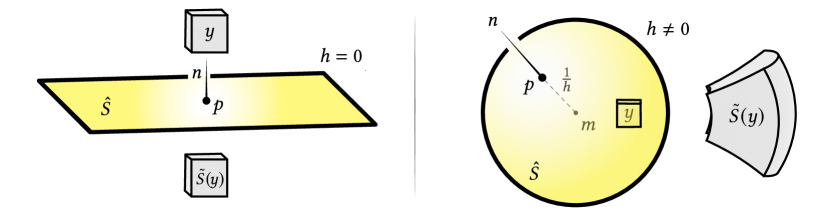
Abbildung 4: The inversion in a 2-sphere is well described in terms of a point $p$ on the sphere, its normal at $p$ and its mean curvature $h$. This description works uniformly to describe inversions in round spheres or reflections through planes.

This sphere inversion can be represented as matrix multiplication by

(23) $$\mathsf{S}=\begin{pmatrix}n&0\\ -h&-n\end{pmatrix}.$$

Indeed, it is easy to verify that

(24) $$\mathsf{S}\begin{pmatrix}y\\ 1\end{pmatrix}=\begin{pmatrix}\tilde{S}(y)\\ 1\end{pmatrix}(-hy-n).$$

By conjugating $\mathsf{S}$ by the Möbius transformation $\mathsf{T}_{p}$ describing translation by $p$ we deduce that the inversion in the oriented sphere in $\mathbb{R}^{3}$ with mean curvature $h$ that passes through the point $p\in\mathbb{R}^{3}$ and at $p$ has unit normal $n$ is represented by the matrix

(25) $$\mathsf{S}=\mathsf{T}_{p}\begin{pmatrix}n&0\\ -h&-n\end{pmatrix}\mathsf{T}_{p}^{-1}.$$

A direct computation shows that all of the matrices describing sphere inversions satisfy $\operatorname{tr}_{\mathbb{R}}\mathsf{S}=0$, $\mathsf{S}^{*}=\mathsf{S}$, and $\mathsf{S}^{2}=-\mathsf{I}$. Conversely, these three equations characterize all of the inversions in 2-spheres in $S^{3}$. In Appendix A.1, we show that any such matrix describes an oriented 2-sphere in $S^{3}$ and that we can identify the space

(26) $$\mathcal{S}\coloneqq\big{\{}\mathsf{S}\in\mathbb{H}^{2\times 2}\,\,\mid\,\,\operatorname{tr}_{\mathbb{R}}\mathsf{S}=0,\,\mathsf{S}^{*}=\mathsf{S},\,\mathsf{S}^{2}=-\mathsf{I}\big{\}}\subset{\operatorname{M\ddot{o}b}}(3).$$

with the space of oriented $2$-spheres in $S^{3}$.

Remark 2.4.

One can recover the sphere from the eigenlines of the linear operator $\mathsf{S}$: that is, $\hat{S}=\{\psi\mathbb{H}\in S^{3}\,\,\mid\,\,\langle\mathsf{S}\psi,\psi\rangle=0\}$. Moreover, $B(\mathsf{S})=\{\psi\mathbb{H}\in S^{3}\,\,\mid\,\,\langle\mathsf{S}\psi,\psi\rangle<0\}$ is an open ball in $S^{3}$. Both $\mathsf{S}$ and $-\mathsf{S}$ determine the same round 2-sphere, but they bound complimentary round balls in $S^{3}$ since $\overline{B(-\mathsf{S})}=S^{3}\setminus B(\mathsf{S})$. Taking this round ball bounded by $\hat{S}$ as its interior determines the orientation of the 2-sphere.

Space of circles

Just as we identified spheres with the inversion in them we now identify circles with the Möbius transformation which, restricted to any 2-sphere containing the circle is an inversion in the circle. Since this is a Möbius geometric definition, we may transform the circle into a line by sending a point on the circle to infinity. Any sphere containing the circle will then be sent to a plane containing the line. The definition of the inversion in the line states that the restriction to any plane containing the line is equal to the reflection about the line. In other words, the inversion in a line is $180^{\circ}$ rotation around the line. By reversing the Möbius transformation mapping the circle into the line we see that the inversion in a circle can also be thought of as a $180^{\circ}$ rotation around the circle. Figure 5 (left) illustrates the $180^{\circ}$ degree rotation around an oriented line in $\mathbb{R}^{3}$ that coincides with the Euclidean rotation about the line. Figure 5 (right) illustrates the $180^{\circ}$ rotation about the oriented circle defined as the rotation around the oriented line that the circle transforms into by sending one of the points on the circle to infinity.

Abbildung 5: It is useful to describe the $180^{\circ}$ rotation around a circle (or line) in $S^{3}$ in terms of a point $p$ on the circle, its tangent at $p$, and its curvature binormal.

In the case when the circle in $S^{3}$ is a line in $\mathbb{R}^{3}$ it is easy to see that the $180^{\circ}$ rotation around the line can also be computed as the composition of the inversion in two planes orthogonally intersecting in the line and that this doesn’t depend on the choice of planes. Möbius geometrically, this means that inversion in a circle can be computed as the composition of the inversions in any two spheres orthogonally intersecting in the circle. This can be done explicitly by using the identification of the space of oriented spheres with $\mathcal{S}$.

Consider an oriented circle in $\mathbb{R}^{3}$ passing through the origin with unit tangent $t$ and mean curvature vector $\kappa n$. We can write the $180^{\circ}$ rotation about the circle as the orthogonal intersection of the sphere

(27) $$\mathsf{S}=\begin{pmatrix}n&0\\ \kappa&-n\end{pmatrix}$$

and the plane defined by the binormal $b=t\times n$

(28) $$\mathsf{P}=\begin{pmatrix}-b&0\\ 0&-b\end{pmatrix}.$$

The $180^{\circ}$ degree rotation $C$ about the circle is the composition of the reflection in the plane $P$ and the inversion $S$ in the sphere:

(29) $$\mathsf{C}=\mathsf{S}\mathsf{P}=\begin{pmatrix}t&0\\ -\kappa b&t\end{pmatrix}.$$

To describe a circle that instead passes through a point $p\in\mathbb{R}^{3}$ instead of the origin, the $180^{\circ}$-rotation around the circle will be given by

(30) $$\mathsf{C}=\mathsf{T}_{p}\begin{pmatrix}t&0\\ -\kappa b&t\end{pmatrix}\mathsf{T}_{p}^{-1}.$$

A direct computation shows that all such matrices satisfy $\mathsf{C}^{*}=-\mathsf{C}$ and $\mathsf{C}^{2}=-\mathsf{I}$. In Appendix A.1 we also show that any such matrix describes an oriented circle in $S^{3}$ and that we can identify the space

(31) $$\mathcal{C}\coloneqq\big{\{}\mathsf{C}\in\mathbb{H}^{2\times 2}\,\,\mid\,\,\mathsf{C}^{*}=-\mathsf{C},\,\mathsf{C}^{2}=-\mathsf{I}\big{\}}\subset{\operatorname{M\ddot{o}b}}(3).$$

with the space of oriented circles in $S^{3}$.

Notice also that $\mathcal{C}\subset\mathfrak{sp}(1,\mkern-1.0mu1)$, allowing us to interpret an element $\mathsf{C}\in\mathcal{C}$ also as an infinitesimal Möbius transformation, generating the one-parameter group of rotations around the oriented circle. Figure 6 visualizes the Möbius vector field $\mathsf{V}_{\mathsf{C}}$ describing the infinitesimal rotation around a circle $\mathsf{C}\in\mathcal{C}$. The orientation of the circle is encoded in the sign of $\mathsf{C}$ since the vector fields $\mathsf{V}_{-\mathsf{C}}=-\mathsf{V}_{\mathsf{C}}$ differ by a sign and so the 1-parameter family of rotations they generate describe the rotations around the circle in two opposite directions.

Abbildung 6: The orientation of a circle associated with $\mathsf{C}\in\mathcal{C}$ can be determined by looking at the Möbius vector field $\mathsf{V}_{\mathsf{C}}$ it generates. The vector field describes an infinitesimal rotation around the circle or line and the orientation is chosen so that the rotation is clockwise around the circle.

Space of point pairs

Lastly, we identify each pair of points with the Möbius transformation that when restricted to any circle containing the two points is an inflection in the pair of points. We can first map the point pair to the origin and infinity by a Möbius transformation. All of the circles containing the point pair are mapped into lines going through the origin and the inversion in the pair of points is now just the Euclidean inversion $x\mapsto-x$. This does not depend on the choice of Möbius transformation used to send the point pair to the origin and infinity since the Euclidean inversion is invariant under all stretch rotations (the subgroup of Möbius transformations fixing the origin and infinity).

Abbildung 7: An inversion in a pair of points is the Möbius transformation defined so that the restriction on every circle containing the two points is the inversion in a pair of points in $S^{1}$. When both of the points are in $\mathbb{R}^{3}$ the inversion in them can be expressed in terms of one of the points $p_{1}$ and the difference of the point positions $p_{2}-p_{1}$.

To determine an explicit expression for the inversion $\mathsf{U}\in\mathbb{H}^{2\times 2}$ in a pair of points $(p_{1},p_{2})\in\mathbb{R}^{3}\times\mathbb{R}^{3}$, $p_{1}\neq p_{2}$, let $\mathsf{p}_{i}=\begin{pmatrix}p_{i}\\ 1\end{pmatrix}\mathbb{H}$ for $i=1,2$. As a linear operator acting on homogeneous coordinates, $\mathsf{U}$ is defined by its action on a basis of $\mathbb{H}^{2}$. Define the action of $\mathsf{U}$ on $\mathsf{p}_{1}$ to be equal to minus the identity and the action of $\mathsf{U}$ on $\mathsf{p}_{2}$ to be equal to the identity. This clearly defines a Möbius transformation that is Möbius invariantly associated with the pair of points, and one can readily check that it agrees with the inversion in the pair of points by sending them to the canonical locations of the origin and infinity. Starting from the explicit ansatz

(32) $$\mathsf{U}=\mathsf{T}_{p_{1}}\begin{pmatrix}1&0\\ 2(p_{2}-p_{1})^{-1}&-1\end{pmatrix}\mathsf{T}_{p_{1}}^{-1}$$

it is straightforward to verify that $\mathsf{U}|_{\mathsf{p}_{1}}=-\mathsf{I}$ and $\mathsf{U}|_{\mathsf{p}_{2}}=\mathsf{I}$ by evaluating $\mathsf{U}$ on vectors $\psi_{i}\in\mathsf{p}_{i}$ for $i=1,2$. All such matrices $\mathsf{U}$ associated with oriented point pairs satisfy $\mathsf{U}^{2}=\mathsf{I}$ and $\mathsf{U}^{*}=-\mathsf{U}$. In Appendix A.1 we show that any such matrix describes an oriented point pair in $S^{3}$ and that we can identify the space

(33) $$\mathcal{P}{}\coloneqq\{\mathsf{U}\in\mathbb{H}^{2\times 2}\,\,|\,\,\mathsf{U}^{*}=-\mathsf{U},\,\mathsf{U}^{2}=\mathsf{I}\}\subset{\operatorname{M\ddot{o}b}}(3).$$

with the space of oriented point pairs in $S^{3}$.

The property of this Möbius transformation that enables it to interact well with the inversions in spheres and circles is that the Euclidean inversion can be computed by composing the inversion (reflection) in a plane going through the origin and the $180^{\circ}$ rotation about the line orthogonal to the plane through the origin. Thus, since any pair of points can be sent to zero and infinity by a Möbius transformation this implies that the inflection in two points can be computed as the composition of a sphere inversion and a circle inversion for any sphere-circle pair which intersect orthogonally in the pair of points (see Proposition 2.10).

The space of point pairs also satisfies $\mathcal{P}\subset\mathfrak{sp}(1,\mkern-1.0mu1)$ and so we can interpret each point pair as an infinitesimal Möbius transformation, generating the 1-parameter subgroup of scaling transformations after using a Möbius transformation to send the points to the origin and infinity. In Figure 8 we visualize the vector field $\mathsf{V}_{\mathsf{U}}=-\mathsf{V}_{\mathsf{-U}}$ for the origin-infinity point pair. The vector field is the radial vector, which is a harmonic vector field.

Abbildung 8: Since $\mathcal{P}\subset\mathfrak{sp}(1,\mkern-1.0mu1)$ every element $\mathsf{U}\in\mathcal{P}$ generates a Möbius vector field $\mathsf{V}_{\mathsf{U}}$ that corresponds to an infinitesimal scaling transformation in any affine chart where the pair of points are at zero and infinity.

Since Möbius transformations preserve harmonic vector fields, we deduce that the vector field associated with an oriented point pair $(p_{1},p_{2})$ is also a harmonic vector field on $S^{3}\setminus\{p_{1},p_{2}\}$ with a source and sink at $p_{1}$ and $p_{2}$, respectively. Integral curves of this vector field are visualized in Figure 9.

Abbildung 9: Integral curves of the harmonic vector field associated with an oriented pair of points visualized on a 2-sphere. All of the integral curves are oriented circles going through through the pair of points. The vector field has a source at the point associated with the $-1$ eigenvalue and a sink at the point associated with the $+1$ eigenvalue.

2.3 Light Cone and Infinitesimal Translations

There are two additional spaces that we also need to define inside of $\mathbb{H}^{2\times 2}$: a realization of $S^{3}$ itself inside of $\mathbb{H}^{2\times 2}$ and a space of infinitesimal translations. These spaces naturally arise in the classification of pencils of spheres in Section 2.4. To realize $S^{3}$ inside of $\mathbb{H}^{2\times 2}$ one can take a renormalized limit of the Möbius transformations obtained by inversion in spheres of vanishing radius centered around the points—in this way we can think of each point in $S^{3}$ as a sphere of zero radius.

Light cone model of $S^{3}$

The light cone model of Möbius $S^{3}$ can be realized inside of $\mathbb{H}^{2\times 2}$ by considering the five-dimensional vector space

(34) $$\mathbb{R}^{4,1} \coloneqq\big{\{}\mathsf{Y}\in\mathbb{H}^{2\times 2}\,\,|\,\,\mathsf{Y}^{*}=\mathsf{Y},\,\operatorname{tr}_{\mathbb{R}}\mathsf{Y}=0\big{\}}$$

(35) $$\,=\Big{\{}\begin{pmatrix}a&\beta\\ \gamma&-a\end{pmatrix}\,\,\mid\,\,a\in\mathbb{R}^{3},\,\beta,\gamma\in\mathbb{R}\Big{\}},$$

endowed with the symmetric bilinear form

(36) $$\langle\mathsf{Y},\mathsf{Y}\rangle=-\tfrac{1}{2}\operatorname{tr}_{\mathbb{R}}\big{(}\mathsf{Y}^{2}\big{)}=\|a\|^{2}-\beta\gamma,\qquad\mathsf{Y}=\begin{pmatrix}a&\beta\\ \gamma&-a\end{pmatrix}$$

of signature (4,1). It is classical that the conformal compactification $S^{3}=\mathbb{R}^{3}\cup\{\infty\}$ can be realized as the projectivized light cone in $\mathbb{R}^{4,1}$. Let

(37) $$\mathcal{L}=\{\mathsf{Y}\in\mathbb{R}^{4,1}\,\,\mid\,\,\langle\mathsf{Y},\mathsf{Y}\rangle=0\}$$

then

(38) $$S^{3}\cong\mathcal{L}/\mathbb{R}^{\times}$$

where the action of $\mathbb{R}^{\times}$ on $\mathbb{R}^{4,1}$ is given by scaling.

Remark 2.5.

A direct computation shows that for $\mathsf{A,B}\in\mathbb{R}^{4,1}$, $\tfrac{1}{2}\{\mathsf{A},\mathsf{B}\}=-\langle\mathsf{A},\mathsf{B}\rangle\mathsf{I}$. Therefore, since the space of oriented 2-spheres $\mathcal{S}$ is also a subset of $\mathbb{R}^{4,1}$ it is the Lorentzian unit sphere $\mathcal{S}=\{\mathsf{S}\in\mathbb{R}^{4,1}\,\,\mid\,\,\langle\mathsf{S},\mathsf{S}\rangle=1\}$ inside $\mathbb{R}^{4,1}$.

An explicit isomorphism between these two models of Möbius $S^{3}$ is given by the Euclidean lift into the light cone

(39) $$\Psi_{p}\coloneqq\mathsf{T}_{p}\begin{pmatrix}0&0\\ 1&0\end{pmatrix}\mathsf{T}_{p}^{-1}=\begin{pmatrix}p&\|p\|^{2}\\ 1&-p\end{pmatrix}.$$

It is straightforward to verify that $\langle\Psi_{p},\Psi_{p}\rangle=0$. The point infinity is described by the point

(40) $$\infty_{4,1}\coloneqq\begin{pmatrix}0&1\\ 0&0\end{pmatrix}$$

The map $\begin{pmatrix}p\\ 1\end{pmatrix}\mathbb{H}\mapsto[\Psi_{p}]$, extended so that the image of $\infty$ is $\infty_{4,1}$, defines a conformal isomorphism between our quaternionic projective model of $S^{3}$ and the classical light cone model of $S^{3}$. Equation 39 is called the Euclidean lift since the identification $p\in\mathbb{R}^{3}\mapsto\Psi_{p}\in\mathbb{R}^{4,1}$ is an isometry. All other lifts into the positive light cone are obtained by multiplying $\Psi_{p}$ by a positive scalar.

Infinitesimal translations

To describe geodesic motion inside a parabolic sphere pencil (see Section 2.4) one needs to work with a bundle of infinitesimal Möbius transformations that describe infinitesimal translations when the basepoint is sent to infinity. For each isotropic line $\mathsf{p}\in S^{3}$ define

(41) $$\mathcal{V}_{\mathsf{p}}\coloneqq\big{\{}\mathsf{W}\in\mathfrak{sp}(1,\mkern-1.0mu1)\,\,\mid\,\,\ker\mathsf{W}\supset\mathsf{p},\,\operatorname{im}\mathsf{W}\subset\mathsf{p}\big{\}}.$$

$\mathcal{V}_{\mathsf{p}}$ and $\mathcal{V}_{\mathsf{A}\mathsf{p}}$ are related by conjugation by $\mathsf{A}$ for any $\mathsf{A}\in{\operatorname{M\ddot{o}b}}(3)$. With a little abuse of notation, for a point $p\in\mathbb{R}^{3}$ we will write $\mathcal{V}_{p}$ to denote $\mathcal{V}_{\begin{pmatrix}p\\ 1\end{pmatrix}\mathbb{H}}$. It is straightforward to verify that

(42) $$\mathcal{V}_{p}=\Big{\{}\mathsf{T}_{p}\begin{pmatrix}0&0\\ w&0\end{pmatrix}\mathsf{T}_{p}^{-1}\,\,\mid\,\,w\in\mathbb{R}^{3}\Big{\}}.$$

All matrices on the right-hand side satisfy the kernel and image condition defining $\mathcal{V}_{p}$, and since both the left and right-hand sides of Equation 42 are vector spaces of the same dimension they are equal. Since

(43) $$\mathcal{V}_{\infty}=\Big{\{}\begin{pmatrix}0&w\\ 0&0\end{pmatrix}\,\,\mid\,\,w\in\mathbb{R}^{3}\Big{\}}$$

consists of nilpotent matrices

(44) $$\exp\begin{pmatrix}0&w\\ 0&0\end{pmatrix}=\mathsf{I}+\begin{pmatrix}0&w\\ 0&0\end{pmatrix}=\mathsf{T}_{w}$$

and therefore elements of $\mathcal{V}_{p}$ can be identified with infinitesimal translations of $\mathbb{R}^{3}$ after $p\in\mathbb{R}^{3}$ is sent to infinity by a Möbius transformation.

2.4 Configurations of Pairs of 2-Spheres in $S^{3}$

To understand the geometry of rolling spheres in the discrete setting we characterize configurations of pairs of spheres in $S^{3}$ up to Möbius transformation and how they may be mapped into one another through orthogonal trajectories. We accomplish this exploiting the algebraic structure of the space of 2-spheres as described in the previous section.

Abbildung 10: Pairs of circles in $S^{2}$ can always be arranged by a Möbius transformation into a canonical form where the pencil of circles that they generate takes a simple form. Left: if the circles intersect in two points then they generate an elliptic pencil of circles that can be arranged to look like Euclidean lines intersecting in a single point. Middle: if the circles intersect in a single point then they generate a parabolic pencil that can be arranged to look like parallel Euclidean lines. Right: if the circles are disjoint then they generate a hyperbolic pencil that can be arranged to look like Euclidean concentric circles.

To understand the possible configurations of pairs of 2-spheres it is useful to first consider configurations of pairs of circles in $S^{2}$. These can always be arranged by a Möbius transformation into one of three configurations illustrated in Figure 10: they can be (1) lines intersecting in a single point, (2) parallel lines, or (3) concentric circles. These are characterized by the number of intersection points, two, one, and none. More coarsely, configurations of pairs of circles in the plane are Möbius equivalent to either concentric circles or a pair of lines. A completely analogous characterization of configurations of pairs of 2-spheres in $S^{3}$ exists as well: configurations of pairs of 2-spheres in $S^{3}$ can always be arranged by a Möbius transformation into one of the following three situations. They can be

1. planes that intersect in a line

2. parallel planes,

3. concentric spheres.

As in the case of circles in $S^{2}$ the configurations of pairs of 2-spheres are characterized by their intersections: in case (i) the two spheres intersect in a circle and we say that they lie in an elliptic sphere pencil. An elliptic sphere pencil consists of all 2-spheres containing a shared circle. in case (ii) we say that two spheres lie in a parabolic sphere pencil intersecting in only a single point. Such a pencil consists of all 2-spheres going through a shared intersection point with the same normal vector there. Parallel planes form a parabolic sphere pencil with the intersection point at infinity. In case (iii) the two spheres have an empty intersection and we say that they lie in a hyperbolic sphere pencil. Such a pencil consists of all 2-spheres about which a sphere inversion swaps a shared pair of points. Concentric spheres about the origin make up the hyperbolic sphere pencil determined by, and swapping, zero and infinity.

Canonical Form

If the pair of spheres have non-empty intersection then we can use a Möbius transformation to send one of their intersection points to infinity and in the process transform both of the spheres into planes. The planes are either parallel or they intersect in a line.

Abbildung 11: A geometric construction used to show that any pair of disjoint spheres can be arranged by Möbius transformation of $S^{3}$ so that they look like concentric spheres. The dashed line represents the normal circle $\mathsf{N}$ that intersects $\mathsf{S}_{1}$ and $\mathsf{S}_{2}$ orthogonally.

To see that disjoint 2-spheres can be canonically transformed into concentric 2-spheres consider the following construction. Use a Möbius transformation to transform one of spheres into a plane. The second sphere must necessarily still be a round sphere. Let $\mathsf{N}$ be the normal line that intersects the plane and the second sphere orthogonally, and let $\Sigma$ be a further sphere which intersects the normal line, plane and second sphere orthogonally—this can be achieved by making a suitable choice among the spheres centered on the intersection point of the normal line and the plane. Now use a Möbius transformation to send $\mathsf{N}$ and $\Sigma$ to a line and a plane respectively. This transforms the plane and the second sphere into two spheres that intersect a plane (transformed $\Sigma$) along with a normal line to the plane orthogonally. As such, the two spheres must be concentric. For a 2-dimensional illustration see Figure 11.

2.4.1 Parameterizing Pencils of Spheres

In essence the pencil of spheres connecting a pair of spheres $\mathsf{S}_{1},\mathsf{S}_{2}\in\mathcal{S}$ can be parameterized as

(45) $$\mathsf{S}(\theta)=\mathsf{S}_{1}+\theta\,\mathsf{S}_{2}$$

in each of the three cases. Even though $\mathsf{S}(\theta)$ must be normalized to lie in $\mathcal{S}$, the unnormalized version still describes the same Möbius transformation on $S^{3}$. The type of pencil can be determined by the number of points (spheres of zero radius) occurring in the pencil: zero for elliptic, one for parabolic, and two for hyperbolic pencils. Since for spheres $\mathsf{S}\in\mathcal{S}$, $\langle\mathsf{S},\mathsf{S}\rangle=1$ and for points $\Psi\in\mathcal{L}$, $\langle\Psi,\Psi\rangle=0$, the number of points that appear in the pencil can be decided by looking at the sign of the discriminant

(46) $$4\langle\mathsf{S}_{1},\mathsf{S}_{2}\rangle^{2}-4$$

of the quadratic equation

$$0=\langle\mathsf{S}(\theta),\mathsf{S}(\theta)\rangle=1+2\theta\langle\mathsf{S}_{1},\mathsf{S}_{2}\rangle+\theta^{2}.$$

For hyperbolic sphere pencils, the parameterization is only valid for a certain range of $\theta$.

This parameterization of sphere pencils describes geodesics up to parameterization in $\mathcal{S}$. To directly map $\mathsf{S}_{1}$ into $\mathsf{S}_{2}$ in this manner one may use the Möbius transformation

(47) $$\mathsf{Q}=\mathsf{I}-\mathsf{S}_{2}\mathsf{S}_{1}.$$

Indeed, since

$$\mathsf{Q}\mathsf{S}_{1}=\mathsf{S}_{1}+\mathsf{S}_{2}=\mathsf{S}_{2}\mathsf{Q}$$

one finds that $\mathsf{Q}\mathsf{S}_{1}\mathsf{Q}^{-1}=\mathsf{S}_{2}$. To see that this transformation describes motion inside the sphere pencil by orthogonal trajectories we will analyze this transformation for pairs of spheres in each of the three kinds of sphere pencils separately. In all cases $\mathsf{S}_{1}\times\mathsf{S}_{2}$ is an element of $\mathfrak{sp}(1,\mkern-1.0mu1)$ describing the Möbius vector field orthogonal to every sphere of the pencil.

2.4.2 Elliptic Sphere Pencils

Elliptic sphere pencils are the most relevant configuration for the analysis of the discrete Willmore energy.

Suppose $\mathsf{S}_{1},\mathsf{S}_{2}\in\mathcal{S}$ generate an elliptic sphere pencil. Using a Möbius transformation we may assume that they describe planes intersecting in a line through the origin

$$\mathsf{S}_{i}=\begin{pmatrix}n_{i}&0\\ 0&-n_{i}\end{pmatrix}$$

for some choice of $n_{i}\in S^{2}\subset\mathbb{R}^{3}$. Therefore,

$$\mathsf{S}_{1}\mathsf{S}_{2}=-\cos\alpha\,\mathsf{I}+\sin\alpha\,\mathsf{C},$$

where $\alpha\in[0,\pi)$ is the angle between the two planes intersecting in the line $\mathsf{C}$. Here $\mathsf{C}\in\mathcal{C}$ describes the intersection line

$$\mathsf{C}=\begin{pmatrix}t&0\\ 0&t\end{pmatrix}$$

with $t\in S^{2}\in\mathbb{R}^{3}$ the unit vector in the direction $n_{1}\times n_{2}$. Since $\mathsf{C}^{2}=-\mathsf{I}$ we can compute the exponential map in closed form

$$\exp(\theta\,\mathsf{C})=\cos\theta\leavevmode\nobreak\ \mathsf{I}+\sin\theta\leavevmode\nobreak\ \mathsf{C}$$

for $\theta\in\mathbb{R}$. Since these are all diagonal matrices the action of $\exp(\theta\mathsf{C})$ on points in $S^{3}$ is a rotation by $2\theta$ around $\mathsf{C}$. Hence the Möbius transformation $\exp(\frac{\alpha}{2}\mathsf{C})$ transforms $\mathsf{S}_{1}$ onto $\mathsf{S}_{2}$ via orthogonal trajectories. When we say that this describes motion via orthogonal trajectories we mean that the family of spheres

$$\mathsf{S}_{t}=\exp\left(\tfrac{t\alpha}{2}\mathsf{C}\right)\mathsf{S}_{1}\exp\left(-\tfrac{t\alpha}{2}\mathsf{C}\right)$$

from $t=0$ to $t=1$ interpolates between $\mathsf{S}_{1}$ and $\mathsf{S}_{2}$ inside their shared elliptic sphere pencil. Under this mapping, points in $\mathsf{S}_{1}$ follow circular trajectories that are orthogonal to the trajectory of spheres $\mathsf{S}_{t}$ in the sphere pencil. So we have shown

Proposition 2.6.

Let $\mathsf{S}_{1},\mathsf{S}_{2}\in\mathcal{S}$ be two spheres intersecting in a circle $\mathsf{C}$. Then

(48) $$\langle\mathsf{S}_{1},\mathsf{S}_{2}\rangle=\cos\alpha,\qquad\mathsf{S}_{1}\times\mathsf{S}_{2}=\sin\alpha\,\mathsf{C}$$

where $\alpha$ is the intersection angle between the two spheres. Moreover, the rotation around $\mathsf{C}$ by an angle $\alpha$ transforms $\mathsf{S}_{1}$ into $\mathsf{S}_{2}$ and is equal to the Möbius transformation $\exp\big{(}\frac{\alpha}{2}\mathsf{C}\big{)}$.

Applying these insights to the expression $\mathsf{Q}$ we have

$$\mathsf{Q}=\mathsf{I}-\mathsf{S}_{2}\mathsf{S}_{1}=(1+\cos\alpha)\mathsf{I}+\sin\alpha\,\mathsf{C}=2\cos\tfrac{\alpha}{2}\big{(}\cos\tfrac{\alpha}{2}\mathsf{I}+\sin\tfrac{\alpha}{2}\mathsf{C}\big{)}=2\cos\tfrac{\alpha}{2}\exp\big{(}\tfrac{\alpha}{2}\mathsf{C}\big{)}.$$

Since the scale factor is irrelevant, we see that $\mathsf{Q}$ is the Möbius transformation that maps $\mathsf{S}_{1}$ into $\mathsf{S}_{2}$ via orthogonal trajectories.

2.4.3 Parabolic Sphere Pencils

Suppose $\mathsf{S}_{1},\mathsf{S}_{2}\in\mathcal{S}$ generate a parabolic sphere pencil.

Up to a suitable Möbius transformation we may assume that they are parallel planes defined by the same normal vector $n\in\mathbb{R}^{3}$:

$$\mathsf{S}_{i}=\begin{pmatrix}n&2\lambda_{i}\\ 0&-n\end{pmatrix}$$

for distinct $\lambda_{i}\in\mathbb{R}$. Here $\lambda_{i}$ specifies the planes as the $\lambda_{i}$ level sets of $\langle n,\cdot\rangle$. Therefore,

$$\mathsf{S}_{1}\mathsf{S}_{2}=\begin{pmatrix}-1&2(\lambda_{2}-\lambda_{1})n\\ 0&-1\end{pmatrix}=-\mathsf{I}+\hat{\mathsf{n}}.$$

Here $\hat{\mathsf{n}}\in\mathcal{V}_{\infty}$ is already an infinitesimal translation since the shared intersection point is at infinity. Since $\hat{\mathsf{n}}$ is nilpotent

$$\exp(\theta\hat{\mathsf{n}})=\mathsf{I}+\theta\hat{\mathsf{n}}=\begin{pmatrix}1&2\theta(\lambda_{2}-\lambda_{1})n\\ 0&1\end{pmatrix}$$

is a translation by $2\theta(\lambda_{2}-\lambda_{1})$ in the direction from the plane $\mathsf{S}_{1}$ to $\mathsf{S}_{2}$. In particular, $\exp\tfrac{\hat{\mathsf{n}}}{2}$ describes the translation mapping $\mathsf{S}_{1}$ to $\mathsf{S}_{2}$ and so we have shown

Proposition 2.7.

Let $\mathsf{S}_{1},\mathsf{S}_{2}\in\mathcal{S}$ be spheres intersecting in a single point $p\in S^{3}$ with the same oriented normal there. Then

$$\langle\mathsf{S}_{1},\mathsf{S}_{2}\rangle=1\qquad\mathsf{S}_{1}\times\mathsf{S}_{2}=\hat{\mathsf{n}}\in\mathcal{V}_{p}$$

and $\hat{\mathsf{n}}$ is an infinitesimal translation when $p$ is sent to infinity and $\exp\tfrac{\hat{\mathsf{n}}}{2}$ is the Möbius transformation mapping $\mathsf{S}_{1}$ to $\mathsf{S}_{2}$ by orthogonal trajectories.

Applying this proposition to the expression $\mathsf{Q}$ we find that

$$\mathsf{Q}=\mathsf{I}-\mathsf{S}_{2}\mathsf{S}_{1}=2\mathsf{I}+\mathsf{S}_{1}\times\mathsf{S}_{2}=2\mathsf{T}_{(\lambda_{2}-\lambda_{1})n}=2\exp\tfrac{\hat{n}}{2}$$

which shows that $\mathsf{Q}$ is the desired Möbius transformation mapping $\mathsf{S}_{1}$ to $\mathsf{S}_{2}$ via orthogonal trajectories.

2.4.4 Hyperbolic Sphere Pencils

Now suppose $\mathsf{S}_{1},\mathsf{S}_{2}\in\mathcal{S}$ describe disjoint oriented spheres that generate a hyperbolic sphere pencil.

By a suitable Möbius transformation we may assume that they are concentric spheres centered at the origin

$$\mathsf{S}_{i}=\begin{pmatrix}0&\lambda_{i}\\ -\tfrac{1}{\lambda_{i}}&0\end{pmatrix}$$

for some choice of $\lambda_{i}\in\mathbb{R}$ for $i=1,2$. The spheres they represent are those defined by $|x|^{2}=|\lambda_{i}|^{2}$.

Note that the orientations of the two spheres must be compatible, in the sense that the signs of $\lambda_{1}$ and $\lambda_{2}$ must be equal. Otherwise there does not exist an orientation preserving Möbius transformation mapping $\mathsf{S}_{1}$ to $\mathsf{S}_{2}$. To avoid these undesirable configurations one needs to assume that the spheres are oriented consistently, and for simplicity, we will take $\lambda_{1},\lambda_{2}>0$. For disjoint spheres that are not in canonical form, consistent orientation is equivalent to the balls bounded by the oriented spheres intersecting in a round ball.

The product of the concentric spheres is

$$\mathsf{S}_{1}\mathsf{S}_{2}=\begin{pmatrix}-\lambda_{1}/\lambda_{2}&0\\ 0&-\lambda_{2}/\lambda_{1}\end{pmatrix}=\cosh\sigma\,\mathsf{I}+\sinh\sigma\,\mathsf{U}$$

with $\sigma=\log\frac{\lambda_{2}}{\lambda_{1}}$ and where $\mathsf{U}\in\mathcal{P}$ is

$$\mathsf{U}=\begin{pmatrix}1&0\\ 0&-1\end{pmatrix},$$

describing the $(0,\infty)$ point pair.

Proposition 2.8.

Let $\mathsf{S}_{1},\mathsf{S}_{2}\in\mathcal{S}$ be disjoint oriented spheres. If the balls bounded by the oriented spheres have non-empty intersection then they generate a hyperbolic sphere pencil defined by a pair of points $\mathsf{U}\in\mathcal{P}$ and

$$\langle\mathsf{S}_{1},\mathsf{S}_{2}\rangle=\cosh\sigma\qquad\mathsf{S}_{1}\times\mathsf{S}_{2}=\sinh\sigma\leavevmode\nobreak\ \mathsf{U}$$

for some $\sigma\in\mathbb{R}$ and $\exp(\tfrac{\sigma}{2}\mathsf{U})$ is the Möbius transformation mapping $\mathsf{S}_{1}$ to $\mathsf{S}_{2}$ by orthogonal trajectories.

Applying this proposition to the expression $\mathsf{Q}$ we find that

$$\mathsf{Q}=\mathsf{I}-\mathsf{S}_{2}\mathsf{S}_{1}=(1+\cosh\sigma)\mathsf{I}+\sinh\sigma\,\mathsf{U}=2\cosh\tfrac{\sigma}{2}(\cosh\tfrac{\sigma}{2}\,\mathsf{I}+\sinh\tfrac{\sigma}{2}\,\mathsf{U})=2\cosh\tfrac{\sigma}{2}\exp(\tfrac{\sigma}{2}\mathsf{U}).$$

This shows that $\mathsf{Q}$ is the desired Möbius transformation that maps $\mathsf{S}_{1}$ to $\mathsf{S}_{2}$ via orthgonal trajectories.

2.5 Möbius Spheres Algebra

After the consideration of products of spheres in the previous section we now consider products of circles and point pairs.

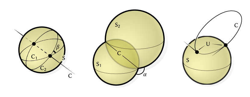
Abbildung 12: Main operations in the algebra of circles, spheres, and point pairs induced by the realizations into $\mathbb{H}^{2\times 2}$.

The following result follows from the same reasoning used to prove Proposition 2.6.

Proposition 2.9.

Let $\mathsf{C}_{1},\mathsf{C}_{2}\in\mathcal{C}$ be two circles that intersect in two points. Their product is

(49) $$\mathsf{C}_{1}\mathsf{C}_{2}=-\langle\mathsf{C}_{1},\mathsf{C}_{2}\rangle\,\mathsf{I}+\mathsf{C}_{1}\times\mathsf{C}_{2}$$

and

(50) $$\langle\mathsf{C}_{1},\mathsf{C}_{2}\rangle=\cos\beta,\qquad\mathsf{C}_{1}\times\mathsf{C}_{2}=\sin\beta\,\mathsf{C}$$

where $\beta$ is the intersection angle of the two circles and $\mathsf{C}$ is the unique circle normal to $S$ at the two intersection points with $S$ the unique sphere containing both $\mathsf{C}_{1}$ and $\mathsf{C}_{2}$.

Proposition 2.10.

Consider a sphere $\mathsf{S}\in\mathcal{S}{}$ along with a pair of points $\mathsf{U}\in\mathcal{P}{}$ contained in $\mathsf{S}$. Then the normal circle $\mathsf{C}\in\mathcal{C}{}$ to the sphere at the two points is equal to the product of the sphere and the point pair

(51) $$\mathsf{C}=\mathsf{S}\mathsf{U}=\mathsf{U}\mathsf{S}.$$

Moreover, $\mathsf{C}\mathsf{S}=\mathsf{S}\mathsf{C}=-\mathsf{U}$ and $\mathsf{S}=\mathsf{C}\mathsf{U}=\mathsf{U}\mathsf{C}$.

Beweis.

It is straightforward to verify that $\mathsf{S}$ and $\mathsf{C}$ commute with $\mathsf{U}$ since the sphere and circle go through the points described by $\mathsf{U}$. From $\mathsf{S}^{*}=\mathsf{S}$ and $\mathsf{U}^{*}=-\mathsf{U}$ we deduce that $(\mathsf{S}\mathsf{U})^{*}=-\mathsf{S}\mathsf{U}$ and that $(\mathsf{S}\mathsf{U})^{2}=-\mathsf{I}$, and so $\mathsf{S}\mathsf{U}\in\mathcal{C}$ and describes a circle going through the points $i$ and $j$. Since the diagonal entries of the matrix representation of a sphere describe its normal vectors, whereas the diagonal entries of a circle describe its tangent vectors, we conclude that $\mathsf{C}=\mathsf{S}\mathsf{U}$ is the desired normal circle orthgonal to $\mathsf{S}$ through the oriented point pair $\mathsf{U}$. ∎

3 Rolling Sphere Connections

With the quaternionic description of spheres in $S^{3}$ in place, it is easy to describe the geometry of a rolling sphere congruence over a surface. In this section we give the geometric interpretation of both the smooth and discrete Willmore energies as the curvature of a connection obtained by rolling spheres over the surface.

Let $f:M\to\mathbb{R}^{3}$ be an immersion of a compact orientable Riemann surface. The mean curvature sphere congruence $\mathsf{S}:M\to\mathcal{S}$ of the immersion is defined to be

(52) $$\mathsf{S}=\mathsf{T}_{f}\begin{pmatrix}n&0\\ -H&-n\end{pmatrix}\mathsf{T}_{f}^{-1}$$

where $H$ is the mean curvature of the immersion, and $n:M\to S^{2}$ is the normal of the immersion. The tangent plane congruence $\mathsf{P}:M\to\mathcal{S}$ is given by

(53) $$\mathsf{P}=\mathsf{T}_{f}\begin{pmatrix}n&0\\ 0&-n\end{pmatrix}\mathsf{T}_{f}^{-1}.$$

Consider the connections $\nabla^{\mathsf{P}}=d-\tfrac{1}{2}\mathsf{P}\,d{\mkern 1.0mu}\mathsf{P}$ and $\nabla^{\mathsf{S}}=d-\tfrac{1}{2}\mathsf{S}\,d{\mkern 1.0mu}\mathsf{S}$ on the trivial $\mathbb{H}^{2}$-bundle over $M$.

The tangent plane congruence is parallel with respect to $\nabla^{\mathsf{P}}$ ($\nabla^{\mathsf{P}}\,\mathsf{P}=0$) and so the trajectories of the induced parallel transport move orthogonally to the tangent planes (see Theorem 3.2). The well-known fact that the curvature of the Levi-Civita connection yields the Gauss curvature form finds its expression in the curvature of $\nabla^{\mathsf{P}}$:

$$R(\nabla^{\mathsf{P}})=-K\mathsf{N}\,\sigma_{f}.$$

Since this is an extrinsic description, a rotation about the normal line $\mathsf{N}$ arises as well.

To extend this picture to the mean curvature spheres we just need to consider the connection $\nabla^{\mathsf{S}}=d-\tfrac{1}{2}\mathsf{S}\,d{\mkern 1.0mu}\mathsf{S}$ instead. Just as before, the mean curvature spheres are parallel with respect to $\nabla^{\mathsf{S}}$ ($\nabla^{\mathsf{S}}\,\mathsf{S}=0$) and so the trajectories of the parallel transport of $\nabla^{\mathsf{S}}$ are orthogonal to the mean curvature spheres. The curvature of $\nabla^{\mathsf{S}}$ will now compute the Willmore integrand

(54) $$R(\nabla^{\mathsf{S}})=(H^{2}-K){\mathsf{N}_{\mathsf{S}}}\,\sigma_{f}.$$

This extrinsic description of the Willmore integrand comes multiplied with $\mathsf{N}_{\mathsf{S}}$, describing the rotation around a normal circle to the immersion.

3.1 Smooth Theory

To study the connections $\nabla^{\mathsf{P}}$ and $\nabla^{\mathsf{S}}$ simultaneously we consider the connection $\nabla^{\Sigma}=d-\tfrac{1}{2}\Sigma\,d\Sigma$ induced by an arbitrary, but otherwise fixed, tangent sphere congruence $\Sigma:M\to\mathcal{S}$. Such a sphere congruence is of the form

(55) $$\Sigma=\mathsf{T}_{f}\begin{pmatrix}n&0\\ -h&-n\end{pmatrix}\mathsf{T}_{f}^{-1}$$

for some smooth function $h:M\to\mathbb{R}$. Since $-\tfrac{1}{2}\Sigma\,d\Sigma\in\Omega^{1}(M;\mathfrak{sp}(1,\mkern-1.0mu1))$ the parallel transport of $\nabla^{\Sigma}$ along a path $\gamma:[0,1]\to M$ is a Möbius transformation $P_{\gamma}\in\mathrm{Sp}(1,1)$ of $S^{3}$.

Abbildung 13: Using the connection $\nabla^{\Sigma}$ to identify infinitesimally close spheres of $\Sigma$ by Möbius transformations we find that the parallel transport of points in $S^{3}$ follows trajectories that are orthogonal to the sphere congruence. Visualized in red is the parallel transport of three points obtained by rolling the tangent plane congruence (right) or a tangent sphere congruence (left) over a sphere.

Proposition 3.1.

The sphere congruence $\Sigma$ is parallel with respect to $\nabla^{\Sigma}$.

Beweis.

Recall that the covariant derivative of an endomorphism field $A\in\Gamma\operatorname{End}\mathbb{H}^{2}$ is defined naturally by $(\nabla^{\Sigma}A)\psi\coloneqq\nabla^{\Sigma}(A\psi)-A\nabla^{\Sigma}\psi.$ For a nowhere vanishing section $\psi:M\to\mathbb{H}^{2}$

(56) $$(\nabla^{\Sigma}\Sigma)\psi =\nabla^{\Sigma}(\Sigma\psi)-\Sigma\nabla^{\Sigma}\psi$$

(57) $$=\big{(}d-\tfrac{1}{2}\Sigma\,d{\mkern 1.0mu}\Sigma\big{)}(\Sigma\psi)-\Sigma\big{(}d-\tfrac{1}{2}\Sigma\,d{\mkern 1.0mu}\Sigma\big{)}\psi$$

(58) $$=d(\Sigma\psi)-\Sigma\,d\psi-\tfrac{1}{2}d{\mkern 1.0mu}\Sigma\,\psi-\tfrac{1}{2}d{\mkern 1.0mu}\Sigma\,\psi$$

(59) $$=0.$$

∎

The geometry of $\nabla^{\Sigma}$ is described by the following result.

Theorem 3.2.

Let $\Sigma$ be a sphere congruence over an interval $[0,1]$ and $\nabla^{\Sigma}$ be the connection on $[0,1]\times\mathbb{H}^{2}$ given by $\nabla^{\Sigma}=d-\tfrac{1}{2}\Sigma\,d\Sigma$. Furthermore, let $\psi\colon[0,1]\to\mathbb{H}^{2}$ be parallel such that $\psi_{0}$ lies on $\Sigma_{0}$. Then $\psi_{t}$ lies on $\Sigma_{t}$ for all $t$ and the trajectory intersects the spheres orthogonally.

Beweis.

Since $\psi_{0}$ lies on $\Sigma_{0}$ we have that $\Sigma_{0}\psi_{0}=-\psi_{0}n_{0}$ where $n_{0}$ is the normal of $\Sigma_{0}$ at $\psi_{0}$. $\Sigma$ is parallel by Proposition 3.1. Since $\psi$ is also parallel

(60) $$\nabla^{\Sigma}_{\frac{\partial}{\partial t}}(\Sigma\psi+\psi n_{0})=0$$

and so by the existence and uniqueness of ODEs $\Sigma_{t}\psi_{t}=-\psi_{t}n_{0}$ for all $t\in[0,1]$.

To simplify subsequent computations we translate everything so that for $t=0$, with

$$\psi_{t}=\begin{pmatrix}{f_{t}}\\ {1}\end{pmatrix}\mu_{t}\qquad\text{we have}\qquad\psi_{0}=\begin{pmatrix}{0}\\ {1}\end{pmatrix}$$

where $f:[0,1]\to\mathbb{R}^{3}$ with $f_{0}=0$. To extract the geometric properties of the trajectory in terms of the curve $f$ we need to determine how $\Sigma$ acts on $\psi^{\prime}$. If we differentiate in time

(61) $$\Sigma^{\prime}\psi+\Sigma\psi^{\prime}=(\Sigma\psi)^{\prime}=\psi^{\prime}(-n_{0}).$$

Since $\psi$ is parallel

(62) $$0=\psi^{\prime}-\tfrac{1}{2}\Sigma\Sigma^{\prime}\psi\implies\Sigma^{\prime}\psi=-2\Sigma\psi^{\prime},$$

and hence by Equation 61 $\Sigma\psi^{\prime}=\psi^{\prime}n_{0}$ . The first row of $\Sigma_{0}\psi_{0}^{\prime}=\psi_{0}^{\prime}n_{0}$ reads $n_{0}f_{0}^{\prime}=f_{0}^{\prime}n_{0}$. Therefore, $f_{0}^{\prime}$ is a scalar multiple of $n_{0}$. Since the point $t=0$ was arbitrary this shows that the trajectory $\psi_{t}$ traced out by parallel transport of $\nabla^{\Sigma}$ is orthogonal to $\Sigma_{t}$ . ∎

The curvature tensor $\mathsf{R}(\nabla^{\Sigma})\in\Omega^{2}(M;\mathfrak{sp}(1,\mkern-1.0mu1))$ is straightforward to compute from the connection 1-form $\nabla^{\Sigma}-d=-\tfrac{1}{2}\Sigma\,d\Sigma$.

Proposition 3.3.

$$\mathsf{R}(\nabla^{\Sigma})=\tfrac{1}{2}\mathsf{T}_{f}\begin{pmatrix}((H^{2}-K)-(H-h)^{2})n\sigma_{f}&0\\ dh\wedge((H-h)df+q)&((H^{2}-K)-(H-h)^{2})n\sigma_{f}\end{pmatrix}\mathsf{T}_{f}^{-1}$$

Beweis.

Let $\mathsf{A}\coloneqq-\tfrac{1}{2}\Sigma\,d{\mkern 1.0mu}\Sigma$ be the connection 1-form of $\nabla^{\Sigma}$. The curvature of the connection is equal to

(63) $$\mathsf{R}(\nabla^{\Sigma})=d{\mkern 1.0mu}\mathsf{A}+\mathsf{A}\wedge\mathsf{A}=-\tfrac{1}{4}d{\mkern 1.0mu}\Sigma\wedge d{\mkern 1.0mu}\Sigma.$$

The derivative of $\Sigma$ is equal to

(64) $$d{\mkern 1.0mu}\Sigma =\mathsf{T}_{f}\left[\begin{pmatrix}0&{d\mkern-1.0muf}\\ 0&0\end{pmatrix}\begin{pmatrix}n&0\\ -h&-n\end{pmatrix}+\begin{pmatrix}dn&0\\ -dh&-dn\end{pmatrix}-\begin{pmatrix}n&0\\ -h&-n\end{pmatrix}\begin{pmatrix}0&{d\mkern-1.0muf}\\ 0&0\end{pmatrix}\right]\mathsf{T}_{f}^{-1}$$

(67) $$=\mathsf{T}_{f}\left(\begin{array}[]{cc}(H-h)\,{d\mkern-1.0muf}+q&0\\ -dh&-(H-h)\,{d\mkern-1.0muf}-q\end{array}\right)\mathsf{T}_{f}^{-1}$$

and since

(68) $$\tfrac{1}{2}{d\mkern-1.0muf}\wedge{d\mkern-1.0muf} =n\,\sigma_{f} \tfrac{1}{2}q\wedge q =-(H^{2}-K)\,n\,\sigma_{f} {d\mkern-1.0muf}\wedge q =q\wedge{d\mkern-1.0muf}=0$$

we have

(69) $$-\tfrac{1}{4}d{\mkern 1.0mu}\Sigma\wedge d{\mkern 1.0mu}\Sigma =\tfrac{1}{2}\mathsf{T}_{f}\begin{pmatrix}((H^{2}-K)-(H-h)^{2})n\sigma_{f}&0\\ dh\wedge((H-h)df+q)&((H^{2}-K)-(H-h)^{2})n\sigma_{f}\end{pmatrix}\mathsf{T}_{f}^{-1}$$

∎

Example 3.4.

That the Gauss curvature can be realized as the curvature of a connection obtained by rolling tangent planes around follows from Proposition 3.3 by taking $h\equiv 0$:

(70) $$\mathsf{R}(\nabla^{\mathsf{P}})=\tfrac{1}{2}\mathsf{T}_{f}\left(\begin{array}[]{cc}-Kn\,\sigma_{f}&0\\ 0&-Kn\,\sigma_{f}\end{array}\right)\mathsf{T}_{f}^{-1}=-\tfrac{1}{2}K\mathsf{N}\,\sigma_{f}$$

where $\mathsf{N}$ describes the congruence of normal lines of $f$.

Example 3.5.

Another consequence of Proposition 3.3 is that the Willmore energy is equal to the curvature of a connection obtained by rolling mean curvature spheres over the surface.

(71) $$\mathsf{R}(\nabla^{\mathsf{S}})=\tfrac{1}{2}\mathsf{T}_{f}\left(\begin{array}[]{cc}(H^{2}-K)\,n\,\sigma_{f}&0\\ dH\wedge q&(H^{2}-K)\,n\,\sigma_{f}\end{array}\right)\mathsf{T}_{f}^{-1}=\tfrac{(H^{2}-K)}{2}\mathsf{N}_{\mathsf{S}}\,\sigma_{f}$$

The normal circle $\mathsf{N}_{\mathsf{S}}$ appears after dividing this 2-form by $\sigma_{f}$ and subsequent normalization which is only possible away from umbilic points.

3.2 Discrete Theory

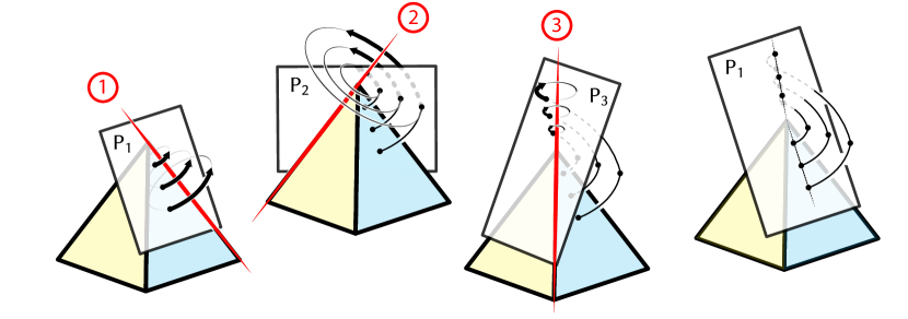
Abbildung 14: A well-known result is that rolling the tangent planes over a discrete surface computes the angle defect, a discrete version of Gaussian curvature. Up to sending the point of rotation to infinity, this picture also describes the Möbius rolling of spheres over a discrete surface. In that case, the monodromy angle computes the discrete Willmore energy instead.

The smooth interpretation of the Willmore energy provides a geometric principle from which one can arrive at a discretization of the Willmore energy. Given an assignment of discrete mean curvature spheres on the vertices of some cell complex define a discrete Willmore energy per face from the monodromy obtained by rolling the discrete mean curvature spheres over the surface. If the discrete mean curvature spheres are Möbius invariantly determined from the discrete surface then the resulting discrete Willmore energy is also Möbius invariant.

In the following section, we show that the discrete Willmore energy from Equation 2 arises in this way from the choice of circumspheres for discrete mean curvature spheres. The circumspheres are defined per edge as the unique sphere containing the four vertices of the two faces adjacent to the edge, and so we introduce the Kagome complex (Section 3.2.2) to describe the combinatorics of rolling adjacent circumspheres. As we roll the circumspheres around a vertex we obtain a Möbius monodromy. Away from the vertices $i\in\mathsf{V}$ where $\mathcal{W}_{i}=0$ the monodromy is a rotation about a normal circle to the circumsphere that we started rolling from. To extract the discrete Willmore energy from this monodromy we only need to look at the rotation angle of this transformation.

3.2.1 Simplicial Surfaces

So that the circumspheres are well-defined we need to assume that the vertices of the triangles incident on an edge are not concircular.

Definition 3.6.

For each face $ijk\in\mathsf{F}$, the circumcircle $\mathtt{C}_{ijk}\in\mathcal{C}$ is the unique oriented circle going through $\mathtt{f}_{i},\mathtt{f}_{j},\mathtt{f}_{k}$ in counterclockwise order.

The geometric properties of the circumcircle can be summarized in the following expression of $\mathtt{C}_{ijk}$ written with respect to the vertex $\mathtt{f}_{i}$:

(72) $$\mathtt{C}_{ijk}=\mathsf{T}_{\mathtt{f}_{i}}\begin{pmatrix}\mathtt{t}_{ijk}^{i}&0\\ -\mathtt{k}_{ijk}&\mathtt{t}_{ijk}^{i}\end{pmatrix}\mathsf{T}_{\mathtt{f}_{i}}^{-1}$$

where $\mathtt{t}_{ijk}^{i}$ is the tangent to the circumcircle $\mathtt{C}_{ijk}$ at the point $\mathtt{f}_{i}$ and $\mathtt{k}_{ijk}$ is the circumcircle curvature binormal.

Definition 3.7.

For each edge $i\mkern-1.0muj\in\mathsf{E}$, the circumcircle intersection angle $\beta_{i\mkern-1.0muj}\in[0,\pi)$ is defined to be the intersection angle between the circumcircles $\mathtt{C}_{ijk}$ and $\mathtt{C}_{jil}$.

The circumcircle intersection angle can be computed from $\cos\beta_{i\mkern-1.0muj}=\langle\mathtt{C}_{ijk},\mathtt{C}_{jil}\rangle$.

Definition 3.8.

For each edge $i\mkern-1.0muj\in\mathsf{E}$, the edge circumsphere $\mathtt{S}_{i\mkern-1.0muj}$ is defined to be the unique sphere containing the circumcircles $\mathtt{C}_{ijk}$ and $\mathtt{C}_{jil}$. The orientation of $\mathtt{S}_{i\mkern-1.0muj}$ is determined so that the outward pointing normal to $\mathtt{S}_{i\mkern-1.0muj}$ at the points $\mathtt{f}_{i}$ is given by the direction of the cross-product of the tangent vectors of the circumcircles $\mathtt{t}_{jil}^{i}\times\mathtt{t}_{ijk}^{i}$.

We will later also need to refer to the geometric properties of the circumsphere that are summarized in the following expression for $\mathtt{S}_{i\mkern-1.0muj}$:

(73) $$\mathtt{S}_{i\mkern-1.0muj}=\mathsf{T}_{\mathtt{f}_{i}}\begin{pmatrix}\mathtt{n}_{i\mkern-1.0muj}^{i}&0\\ -h_{i\mkern-1.0muj}&-\mathtt{n}_{i\mkern-1.0muj}^{i}\end{pmatrix}\mathsf{T}_{\mathtt{f}_{i}}^{-1}$$

where $\mathtt{n}_{i\mkern-1.0muj}^{i}$ is the normal to the edge circumsphere $\mathtt{S}_{i\mkern-1.0muj}$ at the point $\mathtt{f}_{i}$ and $h_{i\mkern-1.0muj}$ is its mean curvature. The circumspheres are a natural choice of the discrete mean curvature spheres since they are defined in a Möbius invariant way using the vertex positions. From the point of view of the discrete Willmore energy, they are also the only natural choice since the energy is defined in terms of circumcircle intersection angles and two adjacent circumcircles uniquely determine the circumsphere.

3.2.2 The Kagome Complex

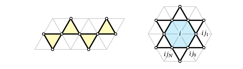
Abbildung 15: The Kagome complex is obtained by connecting up the edge midpoints of the original simplicial surface. The faces of the Kagome complex inside each triangle can be used to express integrability conditions over the triangles, and the faces of the Kagome complex associated with the vertices can be used to express integrability conditions around vertices.

Since the circumspheres live on the edges of $\mathsf{M}$, the Möbius transformations which identify incident circumspheres are most conveniently described as maps that live on the oriented edges of the Kagome complex. The vertices of the Kagome complex are identified with the edges of $\mathsf{M}$ while the edges of the Kagome complex are identified with the corners of $\mathsf{M}$. A corner of $\mathsf{M}$ is described by a face $ijk\in\mathsf{F}$ and a vertex $i$ incident to the face. The faces of the Kagome complex are partitioned into two sets, one is identified with the faces of $\mathsf{M}$ (highlighted in the left side of Figure 15) while the other set is identified with the vertices of $\mathsf{M}$ (highlighted in the right side of Figure 15). We write $j_{ki}$ to denote oriented Kagome edges from $jk$ to $ji$.

The kagome lattice is a two-dimensional geometric lattice structure that has a distinctive pattern of interconnected triangles, reminiscent of a traditional Japanese woven basket called a “kagome.” It is named after this basket due to its resemblance to the interwoven, hexagonal, and equilateral faces seen in the basket’s weave [25]. The Kagome lattice is often used as a theoretical model in condensed matter physics and material science to study phenomena such as magnetism and electron transport [31]. We call our complex the Kagome complex in light of the fact that it generalizes the combinatorics of the Kagome lattice to a triangulated surface.

3.2.3 Rolling Circumspheres

Let us define the rolling circumsphere connection as a discrete $\mathrm{Sp}(1,1)$-connection over the trivial vector bundle over the Kagome complex of $\mathsf{M}$; that is, it is an assignment of a Möbius transformation of $S^{3}$ between fibers $\mathbb{H}^{2}_{i\mkern-1.0muj}=\mathbb{H}^{2}$ and $\mathbb{H}^{2}_{jk}=\mathbb{H}^{2}$ of the trivial $\mathbb{H}^{2}$-bundle over the vertices in the Kagome complex.

Definition 3.9.

The rolling circumspheres connection assigns to each oriented edge $i_{jk}$ in the Kagome complex the map $\mathsf{P}(\nabla^{\mathtt{S}})_{i_{jk}}\in\mathrm{Sp}(1,1)$ defined as

$$\mathsf{P}(\nabla^{\mathtt{S}})_{i_{jk}}\coloneqq\exp\big{(}\tfrac{1}{2}\alpha^{i}_{jk}\mathtt{C}_{ijk}\big{)}$$

where $\alpha^{i}_{jk}$ is the signed angle between the circumspheres $\mathtt{S}_{i\mkern-1.0muj}$ and $\mathtt{S}_{ki}$.

The notation $\mathsf{P}(\nabla^{\mathtt{S}})$ is used to indicate that this is a discrete version of parallel transport induced by the connection $\nabla^{\mathsf{S}}$. The discrete connection can be used to parallel transport points in $S^{3}$ and Möbius transformations of $S^{3}$. Consider a Möbius transformation $A\in\mathbb{H}^{2\times 2}$ of $S^{3}$. It can be parallel transported from $ij$ to $jk$ by conjugation with $\mathsf{P}(\nabla^{\mathsf{S}})_{i_{jk}}$. In particular, if we look at the parallel transport of the circumspheres along Kagome edges we find that circumspheres are parallel:

(74) $$\mathsf{S}_{jk}=\mathsf{P}(\nabla^{\mathsf{S}})_{i_{jk}}\,\mathsf{S}_{i\mkern-1.0muj}\,\mathsf{P}(\nabla^{\mathsf{S}})_{i_{jk}}^{-1}.$$

Since $\mathtt{S}_{i\mkern-1.0muj}$ and $\mathtt{S}_{jk}$ intersect in the circumcircle $\mathtt{C}_{ijk}$ they define an elliptic sphere pencil, and so $\mathsf{I}-\mathtt{S}_{jk}\mathtt{S}_{i\mkern-1.0muj}=2\cos\tfrac{\alpha^{i}_{{jk}}}{2}\leavevmode\nobreak\ \mathsf{P}(\nabla^{\mathsf{S}})_{i_{jk}}$. Since the parallel transport is obtained by rotation around the circumcircle the trajectories traced out by the interpolated parallel transport maps $t\mapsto\exp\big{(}\tfrac{t}{2}\alpha^{i}_{jk}\mathtt{C}_{ijk}\big{)}$ on each edge are orthogonal to the circumspheres (see also Section 2.4.2).

Monodromy of the Rolling Circumspheres Connection

The discrete analog of the curvature of the rolling mean curvature spheres connection is given by the monodromy of the rolling circumsphere connection over the faces of the Kagome complex. The faces of the Kagome complex identified with the faces of $\mathsf{M}$ have trivial monodromy since all of the parallel transport maps involved are given by rotations around the same circumcircle. In particular, the parallel transport maps associated with the oriented edges of these faces commute. For the faces of the Kagome complex identified with vertices of the original mesh, the monodromy of the rolling circumspheres connection is defined as the product of the parallel transport in counterclockwise order across the oriented edges bounding a Kagome face associated with a vertex of $\mathsf{M}$. The computation of this monodromy angle will follow from the following elementary lemma concerning the geometry of spherical polygons.

Lemma 3.10.

Let $n_{0},\dots,n_{m-1}\in S^{2}$ be the vertices of a spherical polygon. Assume that consecutive vertices are not antipodal. The composition of the parallel transport maps on $S^{2}$ between successive vertices is equal to the clockwise rotation around $n_{0}$ by the sum of the exterior angles of the polygon.

Beweis.

For $\ell=0,\dots,m-1$ let $\alpha_{\ell}\in[0,\pi)$ and $t_{\ell}\in S^{2}$ be defined by

(75) $$\cos\alpha_{\ell}=\langle n_{\ell},n_{\ell+1}\rangle,\qquad\sin\alpha_{\ell}\leavevmode\nobreak\ t_{\ell}=n_{\ell}\times n_{\ell+1}$$

where the indices are treated modulo $m$. The exterior angles $\beta_{\ell}\in[0,\pi)$ are defined by

(76) $$\cos\beta_{\ell}=\langle t_{\ell-1},t_{\ell}\rangle.$$

Define the parallel transport rotations as quaternions $\rho_{\ell}\coloneqq\exp(\tfrac{\alpha_{\ell}}{2}t_{\ell})$, which satisfy $\rho_{\ell}n_{\ell}\rho_{\ell}^{-1}=n_{\ell+1}$. Introducing $\sigma_{\ell}\coloneqq\exp(\tfrac{\beta_{\ell}}{2}n_{\ell})$, one obtains that the ordered product

(77) $$\prod_{\ell=0}^{m-1}\rho_{\ell}\sigma_{\ell}=\rho_{m-1}\sigma_{m-1}\cdots\rho_{0}\sigma_{0}=\pm 1$$

since it is a rotation that fixes both $n_{0}$ and $t_{0}$.

Abbildung 16: The quaternions $\rho_{\ell}$ and $\sigma_{\ell}$ defined in the proof of Lemma 3.10 describe the rotations visualized in blue and red, respectively. The axes of rotation are indicated by vectors of the same color.

Computing

(78) $$\rho_{\ell}\sigma_{\ell}\rho_{\ell}^{-1}=\rho_{\ell}(\cos\tfrac{\beta_{\ell}}{2}+\sin\tfrac{\beta_{\ell}}{2}n_{\ell})\rho_{\ell}^{-1}=\cos\tfrac{\beta_{\ell}}{2}+\sin\tfrac{\beta_{\ell}}{2}n_{\ell+1}=\exp\Big{(}\tfrac{\beta_{\ell}}{2}n_{\ell+1}\Big{)}$$

and rearranging yields

(79) $$\rho_{\ell}\sigma_{\ell}=\exp\Big{(}\tfrac{\beta_{\ell}}{2}n_{\ell+1}\Big{)}\rho_{\ell}.$$

By a cyclic application of this equation, we conclude that

(80) $$\prod_{\ell=0}^{m-1}\rho_{\ell}\sigma_{\ell}=\exp\Big{(}\frac{n_{0}}{2}\sum_{\ell=0}^{m-1}\beta_{\ell}\Big{)}\prod_{\ell=0}^{m-1}\rho_{\ell},$$

which implies by Equation 77 that

(81) $$\prod_{\ell=0}^{m-1}\rho_{\ell}=\pm\exp\Big{(}-\frac{n_{0}}{2}\sum_{\ell=0}^{m-1}\beta_{\ell}\Big{)}.$$

The sign of the quaternion is irrelevant to the rotation it describes and since counterclockwise rotation about $n_{0}$ corresponds to a positive angle of rotation the monodromy is a clockwise rotation. ∎

For the remainder of this section, we will fix an interior vertex $i\in\mathsf{V}$ and let $\{j_{\alpha}\}_{\alpha=1}^{N}$ be a labeling of the adjacent vertices in counterclockwise order, with $N$ the degree of $i$. Define the monodromy of $\mathsf{P}(\nabla^{\mathtt{S}})$ around the vertex $i$

(82) $$\mathsf{M}(\nabla^{\mathtt{S}})_{i}\coloneqq\prod_{\alpha=1}^{N}\mathsf{P}(\nabla^{\mathtt{S}})_{i_{j_{\alpha}j_{\alpha+1}}}=\mathsf{P}(\nabla^{\mathtt{S}})_{i_{j_{N}j_{0}}}\cdots\mathsf{P}(\nabla^{\mathtt{S}})_{i_{j_{1}j_{2}}}\mathsf{P}(\nabla^{\mathtt{S}})_{i_{j_{0}j_{1}}}.$$

This depends on the labeling of the vertices, but the monodromy obtained from different choices only differ by conjugation, and so the monodromy angle corresponding to the discrete Willmore energy does not depend on this choice.

Theorem 3.11.

If $\mathcal{W}_{i}\neq 0$ then the monodromy $\mathsf{M}(\nabla^{\mathtt{S}})_{i}$ is a rotation about a normal circle to $\mathtt{S}_{i\mkern-1.0muj_{0}}$ with rotation angle equal to the discrete Willmore energy. If $\mathcal{W}_{i}=0$ then after sending $\mathtt{f}_{i}$ to infinity by a Möbius transformation the monodromy is a translation preserving $\mathtt{S}_{i\mkern-1.0muj_{0}}$.

Beweis.

By sending $\mathtt{f}_{i}$ to infinity we transform all of the circumspheres into planes and the monodromy is transformed into a product of Euclidean rotations that maps $\mathtt{S}_{i\mkern-1.0muj_{0}}$ to itself. Therefore, in this transformed picture $\mathsf{M}(\nabla^{\mathtt{S}})_{i}$ is equal to the composition of a translation and a Euclidean rotation about a normal line $\mathsf{N}_{0}$ to the plane $\mathtt{S}_{i\mkern-1.0muj_{0}}$ through the point $\mathtt{f}_{i}$. The translation can be written as $\exp\mathsf{V}=\mathsf{I}+\mathsf{V}$ for some $\mathsf{V}\in\mathcal{V}_{\mathtt{f}_{i}}$ commuting with $\mathtt{S}_{i\mkern-1.0muj_{0}}$. Hence,

(83) $$\mathsf{M}(\nabla^{\mathtt{S}})_{i}=\exp\Big{(}\tfrac{\Theta}{2}\mathsf{N}_{0}\Big{)}\exp\mathsf{V}.$$

The rotation angle $\Theta$ can be determined by examining the action of $\mathsf{M}(\nabla^{\mathtt{S}})_{i}$ on the vector $\psi_{i}\coloneqq\begin{pmatrix}\mathtt{f}_{i}\\ 1\end{pmatrix}$. On one hand, by Equation 83

(84) $$\mathsf{M}(\nabla^{\mathtt{S}})_{i}\psi_{i}=\exp\Big{(}\tfrac{\Theta}{2}\mathsf{N}_{0}\Big{)}\exp\mathsf{V}\psi_{i}=\exp\Big{(}\tfrac{\Theta}{2}\mathsf{N}_{0}\Big{)}\psi_{i}=\psi_{i}\exp\Big{(}\tfrac{\Theta}{2}n_{0}^{i}\Big{)},$$

where $n_{0}^{i}$ is the normal vector to the circumsphere $\mathtt{S}_{0}$ at the point $\mathtt{f}_{i}$. On the other hand, by Equation 82 we have that

(85) $$\mathsf{M}(\nabla^{\mathtt{S}})_{i}\psi_{i}=\prod_{\alpha=1}^{N}\mathsf{P}(\nabla^{\mathtt{S}})_{i_{j_{\alpha}j_{\alpha+1}}}\psi_{i}=\psi_{i}\prod_{\alpha=1}^{N}\exp\Big{(}\tfrac{\alpha^{i}_{j_{\ell}j_{\ell+1}}}{2}\mathtt{t}_{ij_{\ell}j_{\ell+1}}^{i}\Big{)}$$

By Lemma 3.10

(86) $$\prod_{\alpha=1}^{N}\exp\Big{(}\tfrac{\alpha^{i}_{j_{\ell}j_{\ell+1}}}{2}\mathtt{t}_{ij_{\ell}j_{\ell+1}}^{i}\Big{)}=\pm\exp\Big{(}-\tfrac{n_{0}^{i}}{2}\sum_{\ell=0}^{N}\beta_{ij_{\ell}}\Big{)}.$$

Thus, by equating these two expressions

(87) $$\exp\Big{(}\tfrac{\Theta}{2}n_{0}^{i}\Big{)}=\pm\exp\Big{(}-\tfrac{n_{0}^{i}}{2}\sum_{\ell=0}^{N}\beta_{ij_{\ell}}\Big{)}.$$

Therefore,

(88) $$\mathsf{M}(\nabla^{\mathtt{S}})_{i}=\mp\exp\Big{(}-\tfrac{\mathcal{W}_{i}}{2}\mathsf{N}_{0}\Big{)}\exp\mathsf{V}.$$

∎

This geometric interpretation of the discrete Willmore energy as the rotation angle measured when rolling the circumspheres around a vertex mirrors the geometric interpretation of the smooth energy (see Equation 71). In the discrete case the curvature is an element of $\mathrm{Sp}(1,1)$ while in the smooth setting it is an element of $\mathfrak{sp}(1,\mkern-1.0mu1)$. We conclude the paper by discussing one possibility of how the rolling spheres interpretation of the discrete Willmore energy can be used to obtain a discrete Willmore energy for more general piecewise spherical surfaces.

4 Discussion and Outlook

Möbius Invariant Discrete Surfaces

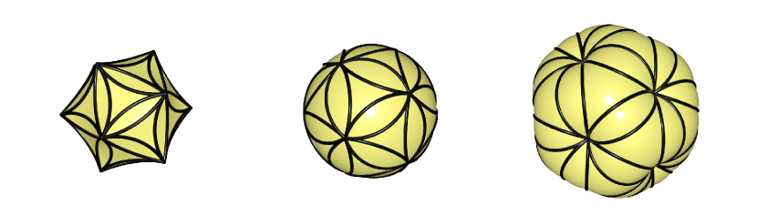
Abbildung 17: Visualized above is the piecewise spherical surface obtained by filling in faces with the ideal hyperbolic triangle determined by the circumcircle and the choice of sphere congruence per face and the edges are filled in with lenses that are uniquely determined from the piecewise spherical regions in adjacent faces.

Given the additional data of a sphere congruence $\mathtt{S}:\mathsf{F}\to\mathcal{S}$ such that $\mathtt{S}_{ijk}$ is in the elliptic sphere pencil generated by the circumcircle $\mathtt{C}_{ijk}$ one can produce a Möbius invariant piecewise spherical surface. That it is Möbius invariant, means that if we transform the vertex positions and sphere congruence by a Möbius transformation then the resulting piecewise spherical surface will transform by the same Möbius transformation.

The construction we present of a piecewise spherical surface from the additional data of a sphere per face consists of two kinds of piecewise spherical faces: (1) ideal hyperbolic faces associated with faces of $\mathsf{M}$ and (2) lens faces associated with edges of $\mathsf{M}$. The ideal hyperbolic faces are obtained by considering the two regions of $\mathtt{S}_{ijk}$ bounded by $\mathtt{C}_{ijk}$ as Poincaré models of two-dimensional hyperbolic space. Using the orientation of both the circumcircle and the sphere $\mathtt{S}_{ijk}$ we can mark the region to the left of the circumcircle as the interior region and we can fill in the vertices $\mathtt{f}_{i},\mathtt{f}_{j},\mathtt{f}_{k}$ with an ideal hyperbolic triangle (which is determined by the three vertices on the ideal boundary) $\Delta_{ijk}$ in the interior Poincaré model of hyperbolic space. For each edge $i\mkern-1.0muj\in\mathsf{E}$ the corresponding boundaries of $\Delta_{ijk}$ and $\Delta_{jil}$ are circular arc edges that intersect in two points $\mathtt{f}_{i},\mathtt{f}_{j}$. As such, there is a unique sphere $\Sigma_{i\mkern-1.0muj}$ containing these two circular arc edges and we can take $\Delta_{i\mkern-1.0muj}$ to be the spherical lens in $\Sigma_{i\mkern-1.0muj}$ interpolating these two circular arc edges. We visualize piecewise spherical surfaces obtained by different choices of sphere congruences in Figure 17. One natural choice is obtained by taking the harmonic mean of the edge circumspheres as the spheres per face; for each face $ijk$:

(89) $$\mathtt{S}_{ijk}\coloneqq\frac{\mathtt{S}_{i\mkern-1.0muj}+\mathtt{S}_{jk}+\mathtt{S}_{ki}}{|\mathtt{S}_{i\mkern-1.0muj}+\mathtt{S}_{jk}+\mathtt{S}_{ki}|}\in\mathcal{S}.$$

With this piecewise spherical surface one can define a geometric discretization of the Willmore energy as the monodromy angle of rolling the face spheres $\mathtt{S}_{ijk}$ onto the edge spheres $\Sigma_{i\mkern-1.0muj}$ and continuing all around a vertex of the original mesh—equivalently, one could consider the area of this discrete sphere congruence. Recently, meshes with spherical faces have also been introduced for applications in architectural geometry [19]. It is an interesting question to study the properties of this energy and the resulting approximation of the Willmore energy obtained by optimizing away the choice of sphere congruence.

Anhang A Möbius Geometry of $S^{3}$

Looking at the components of the equation $\mathsf{A}^{*}\mathsf{A}=\mathsf{I}$ yields the following description of $\mathrm{Sp}(1,1)$:

(90) $$\mathrm{Sp}(1,1)=\Bigg{\{}\begin{pmatrix}a&b\\ c&d\end{pmatrix}\in\mathbb{H}^{2\times 2}\,\,\mid\,\,\operatorname{Re}(a\bar{c})=0,\,\operatorname{Re}(b\bar{d})=0,\,\bar{b}c+\bar{d}a=1\Bigg{\}}$$

Proposition A.1.

Let $\mathsf{A}\in\mathrm{Sp}(1,1)$. Then there exists unique $x,y\in\mathbb{R}^{3}$ and $\mu\in\mathbb{H}$ satisfying

(91) $$\mathsf{A}=\begin{pmatrix}1&0\\ y&1\end{pmatrix}\begin{pmatrix}\mu&0\\ 0&\bar{\mu}^{-1}\end{pmatrix}\begin{pmatrix}1&x\\ 0&1\end{pmatrix}.$$

Beweis.

Let $\mathsf{A}\in\mathrm{Sp}(1,1)$. Then by the characterization from Equation 90 there exists $a,b,c,d\in\mathbb{H}$ satisfying

(92) $$\mathsf{A}=\begin{pmatrix}a&b\\ c&d\end{pmatrix},\qquad\operatorname{Re}(a\bar{c})=0,\,\operatorname{Re}(b\bar{d})=0,\,\bar{b}c+\bar{d}a=1.$$

If $\mathsf{A}$ fixes $\infty$ then $c=0$. Thus, the equation $\bar{b}c+\bar{d}a=\bar{d}a=1$ implies that $d=\bar{a}^{-1}$. Set $\mu=a$, $y=0$, and $x=\bar{d}b$. Since $\operatorname{Re}(b\bar{d})=\operatorname{Re}(\bar{d}b)=\operatorname{Re}(x)=0$ we have that $x\in\mathbb{R}^{3}$ and $\mu x=\mu\mu^{-1}b=b$. Therefore,

(93) $$\begin{pmatrix}1&0\\ y&1\end{pmatrix}\begin{pmatrix}\mu&0\\ 0&\bar{\mu}^{-1}\end{pmatrix}\begin{pmatrix}1&x\\ 0&1\end{pmatrix}=\begin{pmatrix}\mu&\mu x\\ 0&\bar{\mu}^{-1}\end{pmatrix}=\begin{pmatrix}a&b\\ 0&d\end{pmatrix}$$

showing the desired representation for elements of $\mathrm{Sp}(1,1)$ fixing $\infty$.

If $\mathsf{A}$ does not fix $\infty$ then define $p_{\infty}\in\mathbb{R}^{3}$ by $\mathsf{A}\begin{pmatrix}1\\ 0\end{pmatrix}\mathbb{H}=\begin{pmatrix}p_{\infty}\\ 1\end{pmatrix}\mathbb{H}$ and set

(94) $$\tilde{\mathsf{A}}=\begin{pmatrix}1&0\\ -p_{\infty}^{-1}&1\end{pmatrix}\mathsf{A}.$$

Since $\tilde{\mathsf{A}}\begin{pmatrix}1\\ 0\end{pmatrix}\mathbb{H}=\begin{pmatrix}1\\ 0\end{pmatrix}\mathbb{H}$ we can apply the results above to find $\mu\in\mathbb{H}$ and $x\in\mathbb{R}^{3}$ satisfying

(95) $$\tilde{\mathsf{A}}=\begin{pmatrix}\mu&0\\ 0&\bar{\mu}^{-1}\end{pmatrix}\begin{pmatrix}1&x\\ 0&1\end{pmatrix}.$$

Multiplying both sides of the equation by $\begin{pmatrix}1&0\\ p_{\infty}^{-1}&1\end{pmatrix}$ gives the desired representation with $y=p_{\infty}^{-1}$

(96) $$\mathsf{A}=\begin{pmatrix}1&0\\ p_{\infty}^{-1}&1\end{pmatrix}\begin{pmatrix}\mu&0\\ 0&\bar{\mu}^{-1}\end{pmatrix}\begin{pmatrix}1&x\\ 0&1\end{pmatrix}.$$

∎

A.1 Quaternionic Realizations of the Space of $p$-spheres

In this appendix, we will prove that the equations determined in Section 2 that define the spaces $\mathcal{S}$, $\mathcal{C}$, and $\mathcal{P}$ precisely correspond to the inversions in oriented spheres, circles, and point pairs, respectively. The following result will be used to show that the matrices can be assumed to take a simple form where the elementary geometric properties of the spheres can be read off directly from the matrix entries.

Theorem A.2.

If $\mathsf{A}\in{\operatorname{M\ddot{o}b}}(3)$ fixes all points of $S^{3}$ then $\mathsf{A}=\pm\mathsf{I}$.

Beweis.

We first show that the claim holds if $\mathsf{A}\in\mathrm{Sp}(1,1)$ then we show that there does not exist any orientation reversing Möbius transformation satisfying the assumption in the theorem.

Let $\mathsf{A}\in\mathrm{Sp}(1,1)$ be a matrix that fixes all points in $S^{3}$. In particular, it fixes both zero and infinity and so $\mathsf{A}$ is a diagonal matrix of the form

(97) $$\mathsf{A}=\begin{pmatrix}a&0\\ 0&\bar{a}^{-1}\end{pmatrix}$$

for some $a\in\mathbb{H}$. For all $y\in\mathbb{R}^{3}$ we have that

(98) $$\mathsf{A}\begin{pmatrix}y\\ 1\end{pmatrix}=\begin{pmatrix}ay\\ \bar{a}^{-1}\end{pmatrix}=\begin{pmatrix}y\\ 1\end{pmatrix}\lambda_{y}$$

for some $\lambda_{y}\in\mathbb{H}$. The second row of this equation implies that $\lambda_{y}=\bar{a}^{-1}$ and so the first row of this equation implies that $ay=y\bar{a}^{-1}$ for all $y\in\mathbb{R}^{3}$. Taking the norm of this equation implies that $|a|=1$ and so $\bar{a}^{-1}=a$. Therefore, $ay=ya$ for all $y\in\mathbb{R}^{3}$ and so $a\in\mathbb{R}$. The condition that $|a|=1$ implies that $a=\pm 1$ and so $\mathsf{A}=\pm\mathsf{I}$.

If $\mathsf{A}\in{\operatorname{M\ddot{o}b}}(3)$ describes an orientation reversing Möbius transformation of $S^{3}$ then $\mathsf{A}^{*}\mathsf{A}=-\mathsf{I}$. If it fixes all points of $S^{3}$ then it fixes zero and infinity and so

(99) $$\mathsf{A}=\begin{pmatrix}a&0\\ 0&-\bar{a}^{-1}\end{pmatrix}$$

for some $a\in\mathbb{H}$. As above, the assumption that it fixes all points in $S^{3}$ now implies that $ay=-y\bar{a}^{-1}$ and taking the norm of this equation implies that $|a|=1$ and $\bar{a}^{-1}=a$. Thus, $ay=-ya$ for all $y\in\mathbb{R}^{3}$ and this only holds for $a=0$, which obviously cannot hold and so we conclude that no orientation reversing Möbius transformation of $S^{3}$ exists that fixes all points of $S^{3}$. ∎

Proposition A.3.

Let $\mathsf{S}\in\mathcal{S}$. Then $\mathsf{S}$ describes the inversion in a two-sphere in $S^{3}$.

Beweis.

Since $\mathsf{S}^{*}\mathsf{S}=-\mathsf{I}$, by Theorem A.2, then $\mathsf{S}$ does not fix all points of $S^{3}$. Hence two distinct points are interchanged by $\mathsf{S}$. Without loss of generality we can assume that zero and infinity are interchanged, and so

(100) $$\mathsf{S}=\begin{pmatrix}0&a\\ b&0\end{pmatrix}$$

with $a,b\in\mathbb{R}$ and $ab=ba=-1$. So $a=\rho$ and $b=-1/\rho$ with $\rho\in\mathbb{R}$. This is the inversion in a sphere centered at zero with radius $\rho$:

(101) $$\mathsf{S}\begin{pmatrix}x\\ 1\end{pmatrix}\mathbb{H}=\begin{pmatrix}\tfrac{\rho^{2}}{|x|^{2}}x\\ 1\end{pmatrix}\mathbb{H}$$

∎

Proposition A.4.

Let $\mathsf{C}\in\mathcal{C}$. Then $\mathsf{C}$ describes the inversion in a circle in $S^{3}$.

Beweis.

$\mathsf{C}$ cannot fix all points of $S^{3}$ since by Theorem A.2 this would imply that $\mathsf{C}=\pm\mathsf{I}$ and $\pm\mathsf{I}\notin\mathfrak{sp}(1,\mkern-1.0mu1)$. So two distinct points are interchanged by $\mathsf{C}$. Without loss of generality we can assume that zero and infinity are interchanged. Then

(102) $$\mathsf{C}=\begin{pmatrix}0&{a}\\ {b}&0\end{pmatrix}$$

with ${a},{b}\in\mathbb{R}^{3}$ and ${ab}={ba}=-1$. So ${b}=n/\rho$ and ${a}=\rho n$ with $\rho\in\mathbb{R}$ and $n^{2}=-1$. This is the inversion in a circle centered at the origin with curvature binormal $\rho n$:

(103) $$\mathsf{C}\begin{pmatrix}x\\ 1\end{pmatrix}\mathbb{H}=\begin{pmatrix}-\tfrac{\rho^{2}}{|x|^{2}}\bar{n}xn\\ 1\end{pmatrix}\mathbb{H}$$

∎

Proposition A.5.

Let $\mathsf{U}\in\mathcal{P}$. Then $\mathsf{U}$ describes the inversion in a point pair in $S^{3}$.

Beweis.

$\mathsf{U}$ cannot fix all points of $S^{3}$ since by Theorem A.2 this would imply that $\mathsf{U}=\pm\mathsf{I}$ and $\pm\mathsf{I}\notin\mathfrak{sp}(1,\mkern-1.0mu1)$. So two distinct points that are interchanged by $\mathsf{U}$. Without loss of generality we can assume that zero and infinity are interchanged. Then

(104) $$\mathsf{U}=\begin{pmatrix}0&a\\ b&0\end{pmatrix}$$

with $a,b\in\mathbb{R}^{3}$ and $ab=ba=1$. So $b=a^{-1}$. This is the inversion in the pair of points $a$ and $-a$:

(105) $$\mathsf{U}\begin{pmatrix}a\\ 1\end{pmatrix}\mathbb{H}=\begin{pmatrix}a\\ 1\end{pmatrix}\mathbb{H},\qquad\mathsf{U}\begin{pmatrix}-a\\ 1\end{pmatrix}\mathbb{H}=-\begin{pmatrix}-a\\ 1\end{pmatrix}\mathbb{H}$$

∎