Explainable Authorship Identification in Cultural Heritage Applications: Analysis of a New Perspective

Abstract.

While a substantial amount of work has recently been devoted to enhance the performance of computational Authorship Identification (AId) systems, little to no attention has been paid to endowing AId systems with the ability to explain the reasons behind their predictions. This lacking substantially hinders the practical employment of AId methodologies, since the predictions returned by such systems are hardly useful unless they are supported with suitable explanations. In this paper, we explore the applicability of existing general-purpose eXplainable Artificial Intelligence (XAI) techniques to AId, with a special focus on explanations addressed to scholars working in cultural heritage. In particular, we assess the relative merits of three different types of XAI techniques (feature ranking, probing, factuals and counterfactual selection) on three different AId tasks (authorship attribution, authorship verification, same-authorship verification) by running experiments on real AId data. Our analysis shows that, while these techniques make important first steps towards explainable Authorship Identification, more work remains to be done in order to provide tools that can be profitably integrated in the workflows of scholars.

1. Introduction

Authorship Analysis can be broadly defined as “any attempt to infer the characteristics of the creator of a piece of linguistic data” (Juola, 2006, p. 238), where these characteristics include the author’s biographical information (e.g., age group, gender, mother tongue, etc.) and identity. Since the pioneering work of Mosteller and Wallace (1963), the field of authorship analysis has made extensive use of computational methods, thereby contributing to the work of many scholars in the field of cultural heritage and providing them with new tools and perspectives in the study of historical documents of different languages and periods.

One important group of tasks in authorship analysis goes under the name of Authorship Identification (AId), and concerns the study of the true identity of the author of a written document of unknown or disputed paternity. The three main tasks in the AId group are Authorship Attribution (AA), Authorship Verification (AV), and Same-Authorship Verification (SAV). In AA (Koppel et al., 2009; Stamatatos, 2009), given a document $d$ and a set of candidate authors $\{A_{1},\ldots,A_{m}\}$, the goal is to identify the most likely author of $d$ among the set of candidates; AA is thus a single-label multiclass classification problem, where the classes are the authors in $\{A_{1},\ldots,A_{m}\}$. In AV (Stamatatos, 2016), given a candidate author $A$ and a document $d$, the goal is to infer whether $A$ is the real author of $d$ or not; AV is thus a binary classification problem, with $A$ and $\overline{A}$ as the possible classes. In SAV (Corbara et al., 2023b), given two documents $d_{1}$ and $d_{2}$, the goal is to infer whether they are written by the same (possibly unknown) author or not; SAV is thus also a binary classification problem, with SameAuthor and DifferentAuthor as the possible classes. All of these tasks are usually approached as text classification tasks, whereby a supervised machine learning algorithm, using a set of labelled documents, is used to train a classifier to perform the required prediction task.

A close analysis of the AId literature reveals that, while researchers have devoted a lot of effort to test the relative performance of different learning methods in AId tasks, to check the usefulness of different types of features for capturing written style, and to apply the techniques thus developed to a number of AId case studies, little to no attention has been paid to providing users with explanations regarding the predictions of the above algorithms. This is unsatisfactory, since machine-learned classifiers are usually opaque (i.e., they provide predictions but do not provide intuitive explanations of the reasons behind these predictions), and most users of AId systems hardly assign any value to a “bare” automated prediction, and are instead interested in knowing the reason behind the system prediction.

The goal of this work is to make progress towards filling this gap, by carrying out an in-depth analysis of the suitability to the three main AId tasks of a set of well-known general-purpose eXplainable Artificial Intelligence (XAI) methods, i.e., methods for explaining the predictions of a machine-learned system. In doing this, the users of AId systems that we have in mind are scholars working in cultural heritage (such as philologists, historians, linguists), who are typically not machine learning experts. Note that, in this research, our goal is not to devise a new XAI method, but to examine the suitability of existing XAI methods to AId tasks and to the user group identified above.

This paper is organised as follows. After a discussion on (computational) AId and on the importance of explanations for the predictions issued by machine-learned AId systems (Section 2), in Section 3 we survey relevant related work. In Section 4 we explain the three major classes of methods for explaining the predictions of machine-learned systems that we explore in this paper, i.e., feature ranking, transformer probing, and factuals and counterfactuals selection. In Section 5 we explain our experimental setup, while in Section 6 we showcase the application of the aforementioned methods to AId tasks, and analyse their relative benefits for the specific purposes within the cultural heritage domain. Section 7 concludes, pointing at avenues for future research.

2. Background: Authorship identification and the need for explanations

As mentioned in the introduction, AId tasks are usually tackled as text classification problems (Aggarwal and Zhai, 2012), and solved by using supervised machine learning algorithms. For instance, in order to solve the AV task, a machine learning algorithm trains a binary “$A$ vs. $\overline{A}$” classifier using a training set of labelled texts, where the training examples labelled as $A$ are texts by the candidate author and the training examples labelled as $\overline{A}$ are texts by other (ideally, stylistically similar) authors.

Generally speaking, AId techniques attempt to spot the “hand” of a given writer, thus distinguishing their written production from the production of others. The core of this practice, also known as “stylometry” (Holmes, 1998), does not rely on the investigation of the artistic value or the meaning of the written text, but on a quantifiable characterisation of its style. This characterisation is typically achieved via an analysis of the frequencies of linguistic events (also known as “style markers”) occurring in the document of interest, which are assumed to remain more or less constant throughout the production of a given author, while conversely varying substantially across different authors (Juola, 2006, p. 241). These linguistic events are often of seemingly minimal significance (such as the use of a punctuation symbol or a preposition), but are assumed to be out of the conscious control of the writer, and hence to occur in patterns that are hard to consciously modify or imitate.

AId methodologies are profitably employed in many fields, ranging from cybersecurity (Schmid et al., 2015) to computational forensics (Chaski, 2005; Larner, 2014; Perkins, 2015; Rocha et al., 2017); yet another important area of application for AId techniques is the cultural heritage field, which is the focus of the present article. Indeed, researchers might use AId techniques to infer the identity of the authors of texts of literary or historical value, whose paternity is unknown or disputed. In these cases, unknown or disputed authorship may derive from authors attempting to conceal their identity (whether for a desire to remain anonymous or for the malicious intent to disguise themselves as someone else), or simply as a result of the passing of time, which is a common occurrence when dealing with ancient texts (Kabala, 2020; Kestemont et al., 2016; Savoy, 2019; Stover et al., 2016; Tuccinardi, 2017).

While many efforts in AId have focused on testing the accuracy of different learning algorithms (see for example the surveys by Stamatatos (2009); Juola (2006); Grieve (2007), or the annual editions of the popular PAN shared task (Stamatatos et al., 2022; Kestemont et al., 2021)), or on proposing new sets of features that these algorithms could exploit (Corbara et al., 2023b; Sari et al., 2018; Wu et al., 2021), or simply on applying known techniques to case studies of literary interest (Kabala, 2020; Kestemont et al., 2016; Savoy, 2019; Stover et al., 2016; Tuccinardi, 2017), little or no effort has been devoted to endowing these systems with the ability to generate explanations for their predictions.

This fact represents indeed a very important gap in the literature, and a hindrance to a more widespread adoption of these technologies in cultural heritage and other fields. The ability to provide justifications for their own predictions is a very important property for machine-learned systems in general, and even more so when these systems are involved in significant decisions-making processes, such as deciding on the authorship of written documents, with all its legal and ethical implications. We might even claim that an authorship analysis system is almost useless, unless it is endowed with the ability to explain its own decisions. Indeed, when such a system is applied to, say, determining the authorship of an important literary work of controversial paternity (Corbara et al., 2020, 2022; Kestemont et al., 2015; Tuccinardi, 2017), it is paramount that the prediction is presented to the domain experts along with a comprehensive explanation of the reasons why the system made such a prediction. There are two main reasons for this.

The first one is that a domain expert who has devoted a sizeable intellectual effort to determining the authorship of a given document is unlikely to blindly trust the prediction of an automatic system, unless the possibility to examine the reasons of its prediction and/or the inner working of the system is provided (Ribeiro et al., 2016). Indeed, a domain expert might want to check whether the AId system is actually focusing on the writing style of the document under investigation (and on features deemed important by the expert), and that the system is not instead focusing on other possibly misleading aspects of the document, such as its topic. A similar argument can be applied to an automated prediction meant to be used as evidence in a criminal case: in this case, it would be necessary to put the judge and the jurors in the condition to form their own opinion regarding the output of the automatic system, by giving them as much information as possible on the system and on the reasons that have led it to make that specific prediction (Bromby, 2011; Larner, 2014; Halvani, 2021).

The second reason is that, in the case of cultural heritage applications, the knowledge regarding the process of an AId system might inspire the domain expert with new possible working hypotheses that had not been considered before (e.g., by highlighting a linguistic event that prominently occurs in one author’s works but not in the production of other authors). In this regard, it is interesting to note that, in authorship analysis studies, the domain expert and the automatic system often employ complementary methodologies. For instance, when performing authorship analysis for cultural heritage texts, a domain expert may (i) analyse the historical facts described in the text and check whether a certain candidate author could possibly have been aware of these facts; (ii) analyse the stand that a candidate author takes towards a certain issue, and check whether this stand is compatible with what we already know about the author’s ideas; and (iii) in general, bring to bear their knowledge of a given candidate author, of the historical period in which the candidate operated, of the cultural milieu that surrounded the candidate, and decide whether all these are, or are not, compatible with the hypothesis that the candidate may be the real author of the disputed document. Current automatic AId systems can do none of the above. More in general, while the domain expert can use exogenous real-world knowledge (i.e., knowledge external to the document), an automatic AId system is typically only able to use endogenous knowledge (i.e., knowledge extracted from the document – plus potentially some external linguistic knowledge, in the form of dictionaries, or sets of word embeddings, or similar). However, an automatic system is capable of doing fine-grained statistical analyses that would be difficult, or impossible, for any human to perform; stylometric analysis is indeed one such type of analysis, where an automatic system can analyse a huge amount of linguistic traits of apparently minimal significance that, altogether, can define an author’s style. In other words, this “lower-level” analysis of the text provides a useful complement to the “higher-level” analysis that the domain expert carries out.

To summarise, the role of an automatic system in tasks such as AId should not be that of an opaque, cryptic oracle, but that of a tool that supports the domain expert, who is in charge of delivering the final authorship hypothesis. In other words, the automatic system should be integrated within a pre-existing workflow; by doing so, it could be perceived not as an attempt to replace the domain experts, which would understandably elicit a negative reaction on their part, but as an attempt to support them in their job.

There are three main obstacles in devising an explainable AId system. First, the vector space typical of text-related prediction tasks usually has a very high dimensionality; indeed, many of the tools that have been developed in the XAI literature are more suited to the low dimensionality typical of structured data. Second, the linguistic events employed as features in AId tasks are usually of minimal significance (e.g., the occurrence of a specific character 3-gram), a significance that may be hard to grasp for the person to whom the explanation is addressed; this is indeed an intrinsic problem stemming from the different approaches that humans and machines employ when facing AId tasks. The third obstacle (which is inherently related to the first two) is that, in text-related prediction tasks, a prediction is obtained thanks to the contribution of many features, all representing linguistic events of minor importance; in other words, it is difficult to isolate one or few such events that are responsible for the final prediction by themselves. Moreover, as noted by Halvani (2021), the bag-of-features representation, which is usually employed in AId tasks, loses the contextual information of the individual features, making it difficult to understand how such features relate to each other with regard to the final output. This means that presenting the user with a concise explanation of the prediction (in terms of the features that have contributed to it) is usually a very difficult matter.

3. Related work

In recent years, XAI has gained more and more attention in the NLP and text mining communities; see for example the general surveys on XAI by Hamon et al. (2020); Guidotti et al. (2018); Carvalho et al. (2019); Linardatos et al. (2020), the surveys on XAI applied to NLP and text classification by Lertvittayakumjorn and Toni (2019); Danilevsky et al. (2020), and the recent proposals discussed in the works of Rajagopal et al. (2021); Wiegreffe and Pinter (2019); Liu et al. (2019c); Gu et al. (2021).

XAI methods are usually divided into local explainers and global explainers. A local explainer is a method that returns an explanation for a specific prediction of the classifier, while a global explainer explains the behaviour of a classifier in general, with no reference to a specific prediction. Understandably, each approach has its own pros and cons, but both can be used to offer insight in the rationale of a classification decision. Since the two approaches focus on different kinds of information, they can be complementary, and multiple local explanations can be combined to gain a general understanding of the behaviour of the classifier (Boenninghoff et al., 2019; Lundberg et al., 2020).

Despite the growing interest that XAI has witnessed in recent years, little or no attention has been given to its application to AId, possibly also due to the difficulties mentioned at the end of Section 2. Some recent attempts towards providing explanations for the predictions of text classifiers consist of creating a saliency mask (Guidotti et al., 2018), as in, visually displaying the textual elements that have proven most important for the decision of the classifier directly within the document (this is thus an example of a local explainer). For example, when tackling AV for the Epistle to Cangrande, a medieval Latin text traditionally attributed to Dante Alighieri, Corbara et al. (2020) highlight the 90 paragraphs of the Epistle with different colours based on the classification scores obtained when classifying each paragraph individually (see Figure 1); here, the score obtained by a paragraph is thus used as an approximation of how much a paragraph contributes to the final prediction for the entire document. Theophilo et al. (2022) obtain a similar effect at the feature level by adapting the popular LIME algorithm to process character 4-grams. In order to offer an explanation for the decisions of his compression-based SAV algorithms, Halvani (2021) proposes to colour the two texts based on their differences (the higher the discrepancy, the stronger the colour), thus providing an intuitive and straightforward representation of areas of the texts that play a more important role in the prediction. Alternatively, when working with architectures based on neural networks, researchers have focused on the visualisation of the attention weights (Boenninghoff et al., 2019), or by computing the derivative of the output given the embedding of a word in the input (Shrestha et al., 2017).

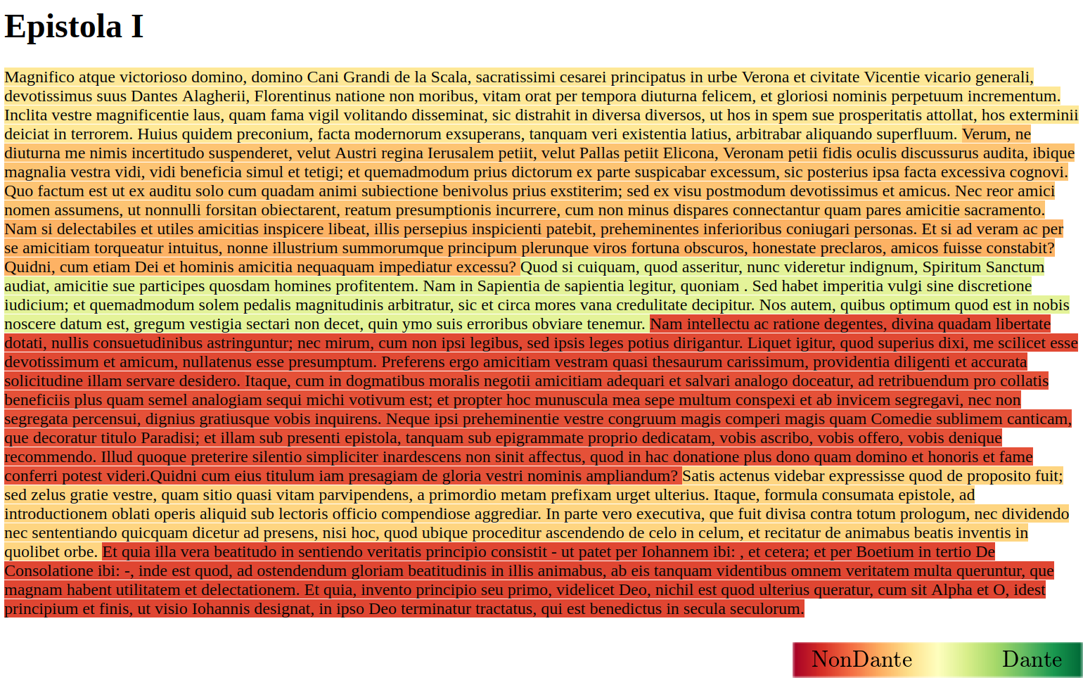
Figure 1. Visualisation of the Epistle to Cangrande (from Corbara et al. (2020)), whose attribution to Dante Alighieri is uncertain; paragraphs on the red side of the spectrum are those that the authorship classifier believes to be “less Dantean”, while those on the green side of the spectrum are those that the authorship classifier believes to be “more Dantean”.

While saliency maps and similar visualisation devices may help the user to focus on areas of the text that have played an important role in the system decision, they are incomplete explanations, since they place on the user the burden of understanding why the system has reached exactly that decision. An alternative method consists of ranking the features used by the classifier by their importance (this is thus an example of a global explainer), where this “importance” can be assessed in different ways. For example, in their work on native language identification (the task of detecting the native language of the author of a text), Berti et al. (2023) use the weights associated to the features in a linear classifier as indications of which features best separate the classes, since the absolute value of these weights is proportional to the discriminative power of the respective features. Other studies, such as the one by Sapkota et al. (2015), assess the effect of different feature types (e.g., character $n$-grams) by evaluating the performance of a classifier trained without the feature types under study. For neural networks, and particularly for CNNs, an approach similar to the above consists of listing the input elements that generate the highest activation values aggregated over all filters, or the input elements that generate a significant activation value for the highest number of filters (Shrestha et al., 2017). However, these approaches are admittedly a long way from constituting satisfactory explanations for AId decisions, because they provide explanations that are partial and/or difficult to grasp for a scholar who is not a machine learning expert.

Another widely used technique consists of displaying the documents of interest in a bidimensional space obtained through dimensionality reduction (e.g., via principal component analysis), in order to provide a visual idea of the characteristics of the data (Binongo, 2003; Forstall et al., 2011; Kestemont et al., 2015). As an example, in Figure 2 texts are mapped to a bidimensional space together with the words whose use most differentiates the candidate authors. A reader is thus able to see how texts by the same author are clustered together, and how the classifier has found the use of specific words to be idiosyncratic to specific authors.

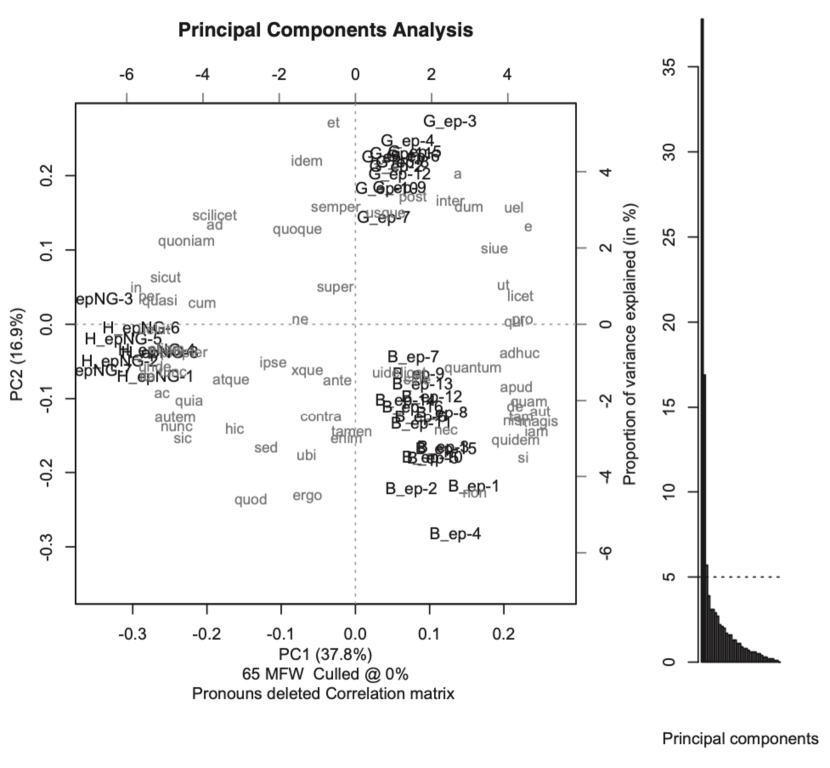
Figure 2. Visualisation (from Kestemont et al. (2015)), obtained via PCA, of texts from three different authors (here identified by the letters B, G, H), showing that the technique used separates them well; strings $A$_ep-$n$ identify the $n$-th text by author $A$ in the dataset. The words that are located near the texts by author $A$ are the ones that occur more frequently in the texts by $A$ than in the texts by the other two authors.

4. Methodology

As briefly discussed in Section 3, there are several general-purpose XAI methodologies that allow to better understand a trained classifier and/or a specific prediction. In this work, we experiment with three of these options, analysing their suitability to AId tasks in general, and to the specific public of cultural heritage professionals in particular. Within this context, we discuss the possible contribution of both global explainers and local explainers.

In Section 4.1 we show how to gain insight into the features that a linear classifier deems most important for the classification task; we do so by directly employing the weights of the trained model, and show how to obtain both global and local explanations. Note that, in the case of linear classifiers, and more generally in the case of “classic” machine learning methods (such as SVMs, logistic regression, decision trees, shallow neural networks), the features used to train the learning algorithm are identified a priori by the researcher, in the so-called “feature engineering” phase. In other words, the model, and thus the explanation, is constrained to use only the features (and combinations thereof) defined by the researcher.

Conversely, deep neural networks are by design able to discover novel discriminative features from the data, and can thus carry out the feature engineering phase autonomously. While some feature ranking solutions for deep-learning models are present in the literature (Lundberg and Lee, 2017), they are extremely sensitive to the input data, and are based on a number of assumptions (such as uniform data distribution) which are often unrealistic (Hooker and Mentch, 2019). Thus, in the case of AId solutions based on deep learning, rather than providing hardly interpretable and/or unreliable explanations, we will thus employ a more sophisticated solution, known as “model probing”, as applied to a RoBERTa-based model, in order to obtain global explanations (see Section 4.2).

Finally, in Section 4.3 we discuss how to extract prototypical examples from the training set. These representative examples provide the user with instances that the model deems most similar to the test example and that belong to the same (or different) class as the model prediction, exposing the internal representation learned by the model, and thus acting as local explainers.

4.1. Feature ranking

A common strategy for offering a global explanation (i.e., providing a general understanding of the behaviour of the classifier) is to show the features the classifier mostly focuses on during prediction, as already explained in Section 3. In these XAI methods, given a trained model, each feature is associated to a score, and the employed features are presented in decreasing order based on their score.

The score of a feature can be obtained in various ways. In the case of linear models, the most direct way is to employ the coefficients (or weights) of the classifier. By design, a linear classifier has the form $h:\mathbf{x}\cdot\mathbf{w}+b$, where $\mathbf{x}$ is the feature vector that represents data item $x$, $\mathbf{w}$ is a vector of weights learned from the training data (one weight for each feature), and $b$ is the intercept of the function; item $x$ is assigned the positive class when $h(\mathbf{x})>0$, and it is assigned the negative class otherwise. In the application scenario we discuss in Section 5.2, where the feature vectors fed to the linear SVM are positive definite, the higher the absolute value of the weight $w_{i}$ associated to the $i$-th feature, the larger is the contribution of such feature towards the prediction.

Note that linear methods compute a set of coefficients for each binary classification problem (which is the case of SAV and AV). In the case of multiclass classification (which is the case of AA), the learner computes a set of coefficients for each class; for prediction explanation purposes, these sets must be examined individually.

The coefficients of the model can also be used to obtain a form of local explanation: by multiplying the feature value extracted from a test example by the correspondent coefficient, we can assess how much the feature determined the specific prediction for the document. This allows us to understand the model both on a global level and on a local level, explaining both how the model generally reasons, and how it reasons on specific instances.

There are more sophisticated ways to get feature scores (and they are a mandatory resource in the case of non-linear methods, such as neural networks). For example, SHAP (Lundberg and Lee, 2017) is a widely used family of algorithms for model-agnostic XAI (meaning that it can be applied to any learning algorithm). Unlike LIME, SHAP performs perturbations on the feature set, then queries the model to estimate the importance of each feature by leveraging the change in prediction that each perturbation has produced on the outcome of the model. By default, SHAP scores are local explanations, but the scores from multiple examples can be averaged to reach a global explanation. However, since the number of features employed in textual settings is usually extremely high, the number of perturbations that the SHAP algorithm should compute would be exponentially large, making it computationally prohibitive; in these cases, perturbations can be approximated through random sampling, but this is only a band-aid solution.

Even though in this case the features employed by the classifier are defined a priori, an explanation of the type described above can be extremely useful for the scholar. For instance, in the tens of thousands character $n$-grams that can be extracted from the texts, what are the most discriminative for the author(s) of interest? Thanks to the explanations mentioned above, in theory a scholar might find out, for example, that a certain author tends to avoid certain patterns of characters, or vice versa has a preference for specific syntactic constructs.

4.2. Probing

As already shown, obtaining an indication of the importance of the features by using the feature weights of the model is straightforward for linear classifiers; however, it is not as straightforward for non-linear classifiers, such as the ones exploiting neural networks. Nevertheless, explainability is even more important for these “black-box” architectures, for at least two reasons. On the one hand, since the features are not identified a priori by the designer (as it is instead the case with “traditional” learners), an explanation method may allow the scholar to check if the classifier is using the features that they indeed deem important for the recognition of authorial style, and thus it might help them to trust the classification system (see Section 2). On the other hand, an explanation method may allow the scholar to check if the system has discovered new features that are interesting for identifying the authorship of written documents, and that can be interesting to investigate further.

Indeed, many recent studies have tackled the far-from-trivial task of developing XAI techniques that can show what features these models are actually leveraging in their predictions. Among these studies, the method of “probing” has recently gained vast popularity (Belinkov, 2022). Probing allows a user to understand if a certain feature of interest (not defined a priori by the designer) has been learned and used by the model. For instance, probing has been used to discover that some famous pre-trained language models, such as BERT and RoBERTa, are not really capable of understanding basic mathematical concepts (Lin et al., 2020), but seem to have learnt some form of common sense directly from data (Jullien et al., 2022). The main idea behind the process of probing is to input the latent representation computed by the neural network model (from now on, the main model) to a second, very simple model (from now on, the probe), whose task is to predict whether the feature of interest is present in the latent representation or not. Given the simplicity of the probe and the complexity of the representation, the underlying assumption is that, if the presence of a feature can be found even with a simple probe, then that feature is encoded by the main model in the latent representation.

Specifically, given a non-linear model $\Phi$ and an hypothesis feature $f$, in order to probe the model (that is, when trying to provide an answer to the question “Does $\Phi$ internally learns from $f$?”), we create a dataset of the form $\{\phi(x_{i}),f(x_{i})\}_{i=1}^{n}$, in which $x_{i}$ is a textual document, $\phi(x_{i})$ is the internal representation of $x_{i}$ created by $\Phi$, and $f(x_{i})$ is a function that characterises $x_{i}$ in terms of the feature $f$. For example, $f(x_{i})$ may be binary, returning 1 or 0 to indicate that a given feature is present or absent in $x_{i}$, respectively. Conversely, $f(x_{i})$ may be categorical, returning a class label in the range $\{1,\ldots,n\}$ when the characteristics of $f$ in $x_{i}$ allow us to distinguish amongst $n$ different groups of documents (see Section 6.2). We then train a linear model with this dataset, and we use the resulting classifier to estimate (e.g., via cross-validation) the extent to which the characteristics encoded by the feature under study are directly learnable from the internal representation of $\Phi$. We repeat this process for every feature we conjecture could be playing a role in the decision function that the model implements.

In particular, in Section 6.2, we exemplify this approach by developing five types of probing:

• POS chains: we probe the model for features extracted from the concatenation of Part-Of-Speech (POS) tags, which are nowadays a standard feature type for AId (see for example Jafariakinabad et al. (2020));

• SQ chains: we probe the model for features extracted from the concatenation of Syllabic Quantities (SQ), which have been first proposed for AId tasks in the Latin language by Corbara et al. (2023b);

• Word lengths: we probe the model for the frequency of word lengths, which have been employed as features in the AId field since the proposal by Mendenhall (1887);

• Function words: we probe the model for the frequency of function words, which are widely employed as features in the AId field (Binongo, 2003; Kestemont, 2014);

• Doc genre: we probe the model for the genre of the document, in order to see whether the model encodes the characteristics of the genre into the latent representation.

Given the generality of the probing approach, any feature type can be easily that the domain expert may find interesting to investigate can be probed.

4.3. Selection of factuals and counterfactuals

Given a prediction $\hat{y}$ on an item $\mathbf{x}$, it might be useful for a domain expert to check what the classifier considers similar items, in order for them to i) understand whether the similarities estimated by the classifier indeed make sense according to what the expert already knows about them (e.g., the classifier considers documents from the same historical period similar), and ii) discover possible similarities among the written documents that the expert might have been unaware of, but the classifier has brought to light.

To this aim, a standard method is to retrieve the training instances that are most similar to $\mathbf{x}$ according to the model. Among these training items, some would have the same class as $\hat{y}$, while others would have a class different from $\hat{y}$; the former are called factuals, and the scholar might find them useful when trying to understand the characteristics of the predicted class, while the latter are called counterfactuals, and they might be useful in allowing the scholar to gauge the minimal requirement for the classifier to predict a class $y\neq\hat{y}$. The similarity of two instances can be computed by applying any standard similarity measure directly to the input vectors in the case of linear models with no internal representation, or to the latent representations of the instances in the case of deep learning models. In the case of a linear model, it is also possible to easily spot the features that most contributed to the similarity of the two items.

5. Experimental setup

In this work, we tackle the three major AId tasks, i.e., Authorship Attribution (AA), Authorship Verification (AV), and Same-Authorship Verification (SAV). We show how some well-known XAI methodologies deal with predictions issued in each of these three tasks on a dataset of medieval Latin (Corbara et al., 2022).

In the following paragraphs, we present our experimental setup, which exemplifies common AId settings. In particular, in Section 5.1 we present the dataset we use, while in Section 5.2 we explain our classification methodology, along with the learning algorithms we employ.

The Python code to replicate our experiments is available at: https://github.com/silvia-cor/XAId

5.1. Dataset

In this study, we employ the dataset developed by Corbara et al. (2022). The authors originally divided it into two sub-datasets, MedLatinEpi and MedLatinLit, both containing works in medieval Latin prose, mostly dating to the 13th and 14th centuries; MedLatinEpi is composed of 294 texts of epistolary genre, while MedLatinLit is composed of 30 texts of various nature, especially literary works and chronicles. For this project we select only 5 authors: Dante Alighieri and Giovanni Boccaccio (who have documents in both the sub-datasets), Pier della Vigna (who is the most prolific author of MedLatinEpi), Benvenuto da Imola and Pietro Alighieri (who are the two most prolific authors remaining in MedLatinLit). We delete the quotations from other authors and the parts in languages other than Latin, both marked in the texts. Following Corbara et al. (2023b), we also divide each text into sentences, where a sentence is made of at least 5 distinct words (we attach shorter sentences to the next sentence in the sequence, or to the previous one in case the sentence is the last one in the document); we use each non-overlapping sequence of 10 consecutive sentences as a textual example. By doing this, we end up with 2,729 text example in total. We randomly split the corpus into a training set ($90\%$ of the examples) and a test set (remaining $10\%$) in a stratified fashion.

For SAV, we do not employ all the pairs of segments that can be created within the training and test sets, since their number would quickly explode and would thus drastically slow down the computation. In particular, given a set of authors $\{A_{1},\ldots,A_{z}\}$, we create $n$ SameAuthor pairs for each author $A_{i}$ (each consisting of two random texts by $A_{i}$), and $m$ DifferentAuthor pairs in total (where a DifferentAuthor pair consists of two random texts by two different authors in $\{A_{1},\ldots,A_{z}\}$); the pairs are unique. In our experiments we set $n$=5,000 and $m$=25,000 for both the training set and the test set; therefore, both the training set and the test set are balanced.

For the AV task, we select the author Dante Alighieri as the author of interest, in line with the experiments in Corbara et al. (2022).

5.2. Learning methods

In this study, we experiment with offering explanations for the output of one representative “classic” machine learning method and for one representative deep learning method in the AId setting.

For the former, we employ a linear Support Vector Machine (SVM), a very popular learner in AId tasks (Zheng et al., 2006; Kestemont et al., 2019); we use the implementation available from the scikit-learn library (Pedregosa et al., 2011). We fine-tune the hyperparameter $C$ (with values in the range $[0.001,0.01,0.1,1,10,100,1000]$) by performing 3-fold cross-validation on the training set. In order to train the algorithm, we compute the TfIdf values of all character n-grams with $n\in\{2,3\}$, which is a common strategy in AId tasks (see for example the 2019 PAN shared task (Kestemont et al., 2019)). We then perform feature selection by selecting the $k$ most relevant features via $\chi^{2}$, with $k=1,000$. We tackle SAV in the style of Corbara et al. (2023a), i.e., we create a single feature vector by computing the absolute difference among the feature values of the two documents that make up the document pair, and label the pair as either SameAuthors or DifferentAuthors.

For the deep-learning experiments, we employ a RoBERTa model (Liu et al., 2019b) from the HuggingFace Transformers library (Wolf et al., 2020) specifically trained with Latin data. We fine-tune the model for 5 epochs on the training set, employing the AdamW optimizer (Loshchilov and Hutter, 2018) with initial learning rate set to $0.0001$ and cross-entropy as the loss. For the SAV task, note that RoBERTa is able to directly classify a sequence of two texts: it is sufficient to concatenate the two texts, separated by the appropriate separator token [SEP]. Note also that RoBERTa works with a fixed maximum length of 512 tokens; we thus truncate the textual samples accordingly.

In Table 1 we report the evaluation results for each model and for each task. As we can see, both algorithms show very high performance in all the tasks. Interestingly, while performing almost on par in the AV task, and better in the SAV task, the RoBERTa transformer performs slightly worse than the SVM classifier in the multi-class setting of AA.

	SVM		RoBERTa
	$Acc$	$F_{1}$	$Acc$	$F_{1}$
SAV	.836	.838	.957	.956
AV	.985	.894	.985	.900
AA	.989	.981	.978	.963

Table 1. Evaluation results for the employed classifiers (SVM and RoBERTa); the metrics employed are accuracy ($Acc$) and $F_{1}$. For SAV and AV, which are binary tasks, $F_{1}$ is defined in the standard way, while for AA, which is a single-label multiclass task, the reported $F_{1}$ values are obtained by macro-averaging (i.e., they are computed as the arithmetic mean of the class-specific $F_{1}$ values). Micro-averaged $F_{1}$ values are not reported here, since micro-averaged $F_{1}$ and accuracy are the same measure in single-label multiclass classification. The best model result for each task is in bold.

6. Tools for explainable authorship identification: A comparative analysis

We here present our results divided by type of explanation, namely feature ranking (Section 6.1), probing (Section 6.2), and factual-counterfactual selection (Section 6.3).

6.1. Feature ranking for SAV

In Table 2 we show the top five and bottom five features by coefficient value for the SVM that we have trained for the SAV task.

$n$-grams	coef
“gab”	0.193
“tto”	0.179
“mac”	0.178
“mbi”	0.175
“aia”	0.171
$\dots$
“auc”	-1.454
“_ai”	-1.586
“ait”	-1.725
“ae_”	-3.976
“ae”	-4.792

Table 2. Bottom 5 and top 5 features of the SVM classifier for the SAV task by coefficient value (coef). White spaces in the feature names are indicated with “_”.

In our case, all the feature values are positive, since we employ TfIdf values, and the intercept is positive as well ($2.29$); thus, features associated with positive weights are important for the positive class (SameAuthor), and features associated with negative weights are important for the negative class (DifferentAuthor). Interestingly, we note a disproportion in the coefficient values among positive and negative weights, where the positive values appear smaller than the negative ones, slowly decreasing from the first position toward the value zero. Also, we note that the two features with the highest negative coefficient values are “ae_” and “ae”, meaning that a discrepancy in the frequency of use of this feature is indeed an indicator that the authors are different or, put it another way, that the frequency of use of these features is pretty stable in the production of an author, and is thus a characteristic trait (either because the author tends to use it a lot, or only rarely) of an author. This specific case might be connected with the transitional phase in medieval Latin where scholars started representing the diphthong “ae” with the single letter “e”, instead of with the two separate letters “ae” as it was written throughout antiquity. A large difference in the frequency of use of these features might thus be an indication that the authors are different, since one of the authors had a preference for “ae” while the other instead preferred “e”.

We can check that the ranked features are indeed useful for the classification by running an ablation experiment, also known as Iterative Removal Of Features (IROF) (Rieger and Hansen, 2020). Firstly, we assess the performance of SVM on the test set when using the entire feature set; we then sequentially remove the feature with the highest absolute coefficient value (by setting the associated weight to zero) from the feature set, then re-evaluate the model on the test set (without re-training it).

That the model performance drops as we iteratively remove features should come as no surprise. However, a good ranking of features that effectively reflects the features importance would cause the performance to degrade much faster (i.e., in less iterations) than any other uninformative ranking. This is shown in Figure 3, in which we compare the drop in performance as a function of the number of features removed, by considering our feature ranking (in blue) versus (10 trials of) the random ranking (in orange). The fact that the model becomes a dummy classifier after removing very few features following our ranking proves that the importance criterion is indeed informative.

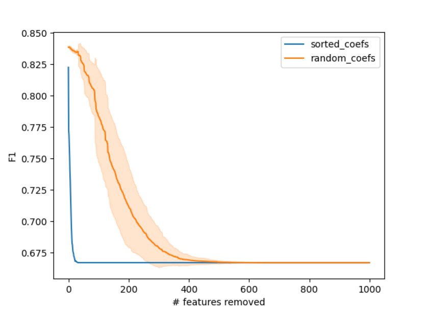
Figure 3. Results of the IROF validation on SVM classifier for SAV: we iteratively remove one feature at a time, following the descending order of the absolute values of the coefficients (sorted_coefs) or a random feature ranking (random_coefs). In particular, for the latter we show the mean $F_{1}$ value obtained at the $n$ feature removed for 10 random feature rankings, where the coloured shadow is the standard deviation.

As already explained in Section 4, we can also employ the coefficients to obtain a form of local explanation, by multiplying the feature value extracted from a document by the correspondent coefficient. We randomly select $2$ examples for each class SameAuthor and DifferentAuthor, and show the results in Figure 4. This visualisation highlights the biggest drawback of this XAI technique when applied to textual examples: if we limit the investigation to just a few features, we might risk to convey an incomplete, and thus wrong, picture, especially to a scholar that is not an expert of machine learning. In fact, what we observe is that, on the basis of these examples, the outcome is often contradictory. Firstly, many of the features displaying positive weights happen to be absent in the selected examples. Secondly, features displaying negative weights behave inconsistently across the examples, e.g., showing relatively high values (examples numbered 2 and 4), or very low values (examples numbered 1 and 3) regardless of their class labels (SameAuthor or DifferentAuthor). Henceforth, it seems clear that restricting the study to only a selected number of features is not enough to convey the full picture of the model behaviour.

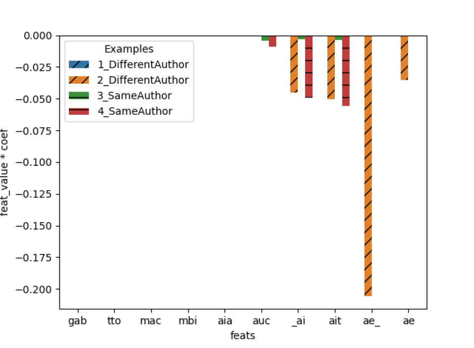
Figure 4. Local explanations for $4$ examples in the test set, given the features listed in Table 2; we colour the SameAuthor class with the ‘-’ pattern and the DifferentAuthor class with the ‘//’ pattern. Note that the scores for many features is zero for all four examples.

Regarding this XAI approach, we can thus conclude that it contributes to justifying the decisions of the system in the eyes of the domain expert to some degree, but it is also rather problematic; as already noted, AId tasks (as any other application of text classification) tend to be characterised by a high number of features, each one providing only a tiny contribution to the final classification decision. In other words, it is unlikely that there are just a handful of features that, by themselves, determine a classification decision. However, as we have shown, limiting the investigation to only a small portion of the features actually employed by the classifier incurs in the risk to convey a picture that is just too narrow and simplistic. Thus, it is of primary importance to offer an analysis that includes the entirety of the feature set used by the classifier in the most user-friendly way possible, allowing a scholar to personalise and navigate the exploration to its full extent.

In particular, a visualisation tool could help display the disputed document with the occurrences of the different features highlighted, with the highlighting coming in different shades depending on the class considered and the significance of the feature. Moreover, the tool could allow the domain expert to select a particular feature of interest, and show one or more dataset examples where the feature has a strong and significant presence.

6.2. Probing the Transformer for AA

In our experiments, we train a simple Logistic Regression model as a probe, since the classification head on top of the RoBERTa transformer has an equivalent complexity, and thus could not gain any more information from the latent representation. We take the training set obtained in Section 5.1 and further split it in a stratified fashion into a training and test set for the probe, consisting of 90% and 10% of the instances respectively. The model hyperparameters are fine-tuned via 3-fold cross-validation on the probe training set. The resulting model is then retrained on the full training set for the probe before evaluation. In our experiments, we probe the main model trained on the AA task.

As illustrated in Section 4.2, we test the transformer with five different probings:

• POS chains: we probe the model for POS chains, where a POS chain is a POS $n$-grams with $n\in\{5,10\}$. In particular, the probe is issued to predict whether a certain POS chain is present ($f(x_{i})=1$) or absent ($f(x_{i})=0$) in the document; the labelling function $f(x_{i})$ is thus binary. We extract the POS tags via the LatinCy pipeline for the SpaCy library. We restrict the analysis to the $5$ most discriminative POS chains in the corpus for the authors classes, computed via $\chi^{2}$.

• SQ chains: the approach is equivalent to the POS chains probing. A SQ chain is a SQ $n$-grams with $n\in\{10,15\}$, and we extract the syllabic quantities via the prosodic scanner in the Classical Language ToolKit (CLTK) library.

• Word lengths: we probe whether the model takes the word-length distribution into account or not. In order to do so, we represent each document $x_{i}$ by means of a histogram $(b_{i}^{(1)},b_{i}^{(2)},\ldots,b_{i}^{(B)})$, in which the bin $b_{i}^{(j)}$ accounts for the relative frequency of words of length $j$ (i.e., the fraction of words of exactly $j$ characters) in the document. Then, we cluster the documents thus represented in order to identify natural groups based on their word-length distribution; we use $k$-means as our clustering algorithm and choose the optimal number of clusters via the Elbow method within the range $[2,10]$. Each cluster is assigned a numerical ID, so that the labelling function $f(x_{i})$ is categorical in this case, and the probe is issued to label each document with the respective $k$-means cluster ID. Note that the histogram representation is only used as a means for deciding the cluster to which each document belongs; that is, the probe is still trained and tested using the internal representations $\phi(x_{i})$ of the model.

• Function words: we create a probe to check the extent to which the model learns from the frequency of use of the function words. To this aim, we apply a strategy that is similar to the aforementioned case for word lengths. That is, we first represent each document $x_{i}$ as a histogram $(b_{i}^{(w_{1})},b_{i}^{(w_{2})},\ldots,b_{i}^{(w_{B})})$, in which the bin $b_{i}^{(w_{j})}$ accounts for the relative frequency of the function word $w_{j}$ in $x_{i}$. We consider the list of 80 function words for Latin used by Corbara et al. (2023b). As before, we label each document with the cluster ID to which it is assigned by a $k$-means algorithm based on the histogram-based representations. The function $f$ is thus again categorical.

• Genre: we probe the model for the genre of the documents; in particular, we ask the probe to classify the documents based on the sub-corpus they belong to, MedLatinEpi or MedLatinLit. As such, we try to asses whether the transformer encodes the stylistic characteristics of documents of epistolary nature ($f(x_{i})=1$) versus documents of literary nature ($f(x_{i})=0$); the labelling function $f(x_{i})$ is thus binary.

We show the results of the POS probing in the first portion of Table 3. The probes show high performance for all the POS chains considered, with the $F_{1}$ performance always above $0.8$, indicating that the transformer is likely learning from the syntax of the documents. These results are in line with the current literature on language model probing (Liu et al., 2019a), and confirm that, even in authorship analysis, models leverage POS chains in downstream tasks. On the other hand, the performance of the SQ probing, displayed in the second portion of Table 3, is quite more limited, scoring values between $0.6$ and $0.7$. However, these results indeed show an actual knowledge by the transformer of the concept of syllabic quantity; this is actually a rather interesting discovery since, to our knowledge, this is the first work in which this kind of information is sought in the latent space generated by a transformer.

	chain	$Acc$	$P$	$R$	$F_{1}$
POS	adj noun adj noun verb	.825	.869	.825	.845
	adj noun noun adj noun	.882	.922	.882	.900
	adp noun adj noun verb	.821	.853	.821	.836
	noun adj noun adj noun	.873	.909	.873	.890
	noun adj noun verb verb	.853	.873	.853	.863
	chain	$Acc$	$P$	$R$	$F_{1}$
SQ	$\cup\cup\cup\cup\cup-\cup\cup\cup\cup$	.670	.684	.670	.674
	$\cup\cup\cup\cup\cup\cup\cup-\cup\cup$	.642	.647	.642	.644
	$\cup\cup\cup\cup\cup\cup\cup\cup\cup-$	.654	.664	.654	.657
	$\cup\cup\cup\cup\cup\cup\cup\cup\cup\cup$	.601	.614	.601	.601
	$\cup\cup\cup\cup\cup\cup\cup\cup\cup\cup\cup$	.626	.670	.626	.639

Table 3. POS and SQ probes results. Probes try to predict the presence of the given POS $n$-gram or SQ $n$-gram in the latent representation of the model. Note that for SQ we here employ the standard notation where $\cup$ stands for a short syllable and $-$ stands for a long syllable.

Regarding word lengths and function words, we show the results of the two multi-class classifications in the first and second portion of Table 4 respectively; interestingly, the optimal number of clusters is $6$ for both experiments. The probe show poor or mediocre results, getting higher scores in inferring the function-words distribution of the documents. This highlights the importance of elements such as function words in the characterisation of literary authors (Kestemont, 2014). We can hypothesise that the fact that the transformer does not seem to encode the information regarding word-lengths distribution could be due to the authors having similar backgrounds, and thus similar habits regarding their vocabulary usage.

	#clusters	$Acc$	$P$	$R$	$F_{1}$
Word lengths	6	.487	.487	.487	.486
Function words	6	.617	.628	.617	.617

Table 4. Word-lengths and function-words probes results. Probes try to predict the word-lengths cluster or function -words cluster in the latent representation of the model.

Regarding probing for the genre of the documents, the results can be seen in Table 5. The probe is clearly able to determine the sub-corpus the document under consideration comes from, thus indicating that the transformer indeed encodes the genre of the document into the latent space. This result could help warn the human expert against the risk that the neural model under investigation might be exploiting domain information, which should be avoided in AId studies (Bischoff et al., 2020; Halvani et al., 2019): the classifier should be focusing on style-related information, and not labelling a document as written by author $A$ simply on the ground that $A$ often writes in the same genre or topic as the document in question.

	$Acc$	$P$	$R$	$F_{1}$
Genre	.979	.979	.979	.979

Table 5. Genre probes results. Probes try to predict the sub-corpus of the documents among MedLatinEpi and MedLatinLit in the latent representation of the model.

Summing up, this analysis could indeed reveal to a scholar some of the inner workings of a high-level model, by showing which features it leverages and which it avoids, thus reassuring the scholar of the outcome of the classification. In particular, the probing task would be well suited for an active interaction with the scholar who, prompted by their deep knowledge on the literary matter, could propose promising features to analyse, in the form of ‘human-in-the-loop” process. However, an important limitation scholars should be aware of, is that the probes can only be constructed around automatically decidable features, unless one wants to incur the cost of manually labelling the documents according to more complicated features.

6.3. Factuals and counterfactuals for AV

In our experiments, we retrieve one factual and one counterfactual for both SVM and RoBERTa trained for the AV task by using the Euclidean distance. Specifically, we obtain the TfIdf vectors (in the SVM case) or the encodings of the final hidden state (in the RoBERTa case) for a random test instance $x$ and the entire training set; we then compute the distances among $x$ and all the training instances, and select the training instance closest to $x$, which has the same (different) label as the predicted label of $x$. Of course, both the number of (counter)factuals outputted and the similarity measure to employ are parameters that can be modified.

The selected test example, which is an epistle from the author Pier della Vigna, is the following:

Fridericus uniuersis mundi principibus de sinistris rumoribus Terrae Sanctae Etsi tam iusta quam uehemens causa doloris et motus fuerit in nobis cum ad presentiam nostram frater S. a uenerabili patre patriarcha Antiocheno dilecto amico nostro presentium baiulus litterarum accessit ipsum tamen infeste uidere nequiuimus qui mittentem affectione quadam diligimus singulari. Uerum etiam tunc temporis cordis nostri neruum pertingerat rumor infestus et subitae nuntius tempestatis qui Coheminorum pestem ab originalibus sedibus Tartarea clade depulsam uelut molem ingentem per abrupta montium et decliuium fulminis ictibus deuolutam in Sanctam Ciuitatem irruisse crudeliter nuntiauit. Quae forte desolationis suae tempore habitatore continui solita defensari cateruatim undique concurrentibus populis colebatur dederatque cursui famosi tamen loci longis retro temporibus a Christicolis maxime desiderata securitas et sinistris auspiciis diebus illis obtenta quarumdam occasione treugarum quas soldanus Damasci et Nathasar soldanus Craci qui prius hostes et aduersarii fuerant concordiam inuicem facientes ipsam cum Christianis ea condicione fecerunt quod tota regni Hierosolimitani terra quam Christiani possederant trans Iordanem retentis sibi uillis et montanis aliquibus restituta Christiani soldanis eisdem in expugnatione soldani Babiloniae deberent assistere toto posse. Qua confederatione tamquam in sui perniciem inita soldanus accinctus predictam gentem Barbaricam Coheminorum per deserta uagantem et uelut feram in saltibus ante uenabulum fugientem ad suae defensionis auxilium conuocauit. qui sibi reputantes oblatum presidium potrius quam petitum ad designata loca subito non minus taciti quam celeres peruenerunt ut inuisos hostes aduenisse maturis nostrorum uigilantia nouerit quam uenturos. sicque factum est ut Christianorum excercitu cum soldanis predictis in guerram soldani Babiloniae apud Gazaram commorante patriarcha Hierosolimitanus de partibus Cismarinis ad partes illas athleta nouus accessit. […]

It is the narration of an episode of the crusade in the Holy Land, with the characteristics of historical chronicles; it is one of the many letters that the author wrote while chancellor of the Emperor Frederick II.

Both SVM and RoBERTa model hold the same factual example, which is again an epistle, but curiously from the author Giovanni Boccaccio:

Celeberrimi nominis militi Iacobo Pizinge serenissimi principis Federici Trinacrie regis logothete. Generose miles incertus mei Neapoli aliquamdiu fueram uere preterito. hinc enim plurimo desiderio trahebar redeundi in patriam quam autumpno nuper elapso indignans liqueram nec minus reuisendi libellos quos immeritos omiseram sic et amicos aliosque caros. inde uero urgebar ut consisterem atque detinebar nunc a uenerabili uiolentia nunc suasionibus nunc precibus incliti uiri Hugonis de comitibus Sancti Seuerini cuius credo splendidam famam noueris. Curabat enim uir eximius etiam me inuito totis uiribus ut me interueniente subsidio serenissime domine Iohanne Ierusalem et sicilie regine apud Parthenopeos placido locaret in otio. qua perplexitate angebar nimium nulla adhuc in parte satis firmato consilio. Et dum sic uariis agitarer curis quo pacto non memini factum tamen est ut ad aures deueniret meas uenerabile nomen religiosi hominis Ubertini de ordine Minorum sacre theologie professoris et conciuis tui cuius auditis meritis eumque ea tempestate Neapoli moram trahere pro quibusdam arduis tui suique regis in desiderium uenit tam conspicuum uidere uirum. a pueritia quippe mea etiam ultra tenelle etatis uires talium auidissimus fui. Nec mora. exhibiturus reuerentiam debitam ad eum accessi atque adaperto capite primo paxillum miratus hominem quam deuotissime et humillime potui salutaui eum. Ipse autem graui quadam maturitate obuius factus me leta facie miti eloquio et morum laudabili comitate suscepit.

In this case, the selected factual is a letter to (ironically!) a notary of the Kingdom of Sicily; the epistle presents a first-person narration, describing some personal occurrences of the author during a staying in Naples. The themes apparently could not be more different from the test example, but at a closer inspection the two texts share many references to religious orders and political relations. We demonstrate this by formatting in bold some of the former and in italic some of the latter.

Regarding the counterfactual, SVM and RoBERTa again hold the same example, which is yet another epistle, this time form the author Dante Alighieri (of course, since in this experiment Dante is the positive class, while all the other authors are the negative class):

Absit a uiro predicante iustitiam ut perpessus iniurias iniuriam inferentibus uelut benemerentibus pecuniam suam soluat. Non est hec uia redeundi ad patriam pater mi. sed si alia per uos ante aut deinde per alios inuenitur que fame Dantisque honori non deroget illam non lentis passibus acceptabo. quod si per nullam talem Florentia introitur nunquam Florentiam introibo. Quidni. nonne solis astrorumque specula ubique conspiciam. nonne dulcissimas ueritates potero speculari ubique sub celo ni prius inglorium ymo ignominiosum populo Florentino ciuitati me reddam. Quippe nec panis deficiet.

Unlike the factual, the counterfactual clearly has a very different domain than the test sample. It is a personal account of the tribulations of returning (unwanted) to one’s homeland. Still, there are again some references to political concepts (again shown in italic).

All in all, it seems that both models are able to spot similarities and differences in the documents, especially the ones linked with the themes and references of the narration. However, spotting these similarities and differences appears to be mainly in the hands of the human user, which could be a long and difficult task. Coupling this XAI technique with other methods that allow to simultaneously enlightening the textual regions, or features, that most determine the similarity among the documents could be helpful in this sense. We give a very elementary exemplification of this by colouring in the texts the $10$ $n$-grams that have the minimum differences among the features values in the test example and in the factual (in blue), and among the features values in the test example and the in counterfactual (in red) (the $n$-grams that are shared among all three texts are coloured in violet).

Other techniques that exist in the related literature generate ad-hoc synthetic examples as (counter)factuals (see for example Lampridis et al. (2022)) . While it might be possible in principle to generate synthetic textual instances for our case too, it is not clear how these examples could be useful for the human expert, who would realistically be interested in real-world textual documents, not machine-generated texts.

7. Conclusion and future works

In this article, we underline the importance of explainability for authorship studies, with a specific focus on the case of cultural heritage. Despite its importance, there are no existing XAI techniques particularly devised for authorship studies in the field of cultural heritage, nor even for generalised applications of authorship analysis. We thus experiment with three existing XAI methodologies proposed in other contexts (namely, feature ranking, probing, and factual and counterfactual selection), and we test them on the three main Authorship Identification tasks (Authorship Attribution, Authorship Verification, and Same-Authorship Verification), employing a medieval Latin dataset as case-study. We make the code here developed available to other researchers that might want to apply these techniques to other authorship problems.

We show that each of the XAI methods partially contributes to understand the reasons behind the predictions of the model, and they jointly provide some sort of explanations of different aspects of the model. In particular, while features ranking and probing shed light on the linguistic events that are leveraged by the model, (counter)factuals put these important linguistic events in context, showing real examples of the writing production under study.

However, we argue that the explanations that can be obtained with current, general-purpose techniques are still largely insufficient, since they either convey a rather limited perspective of the inner working of the classifier (feature ranking) or heavily rely on the user input and intuition (probing, factuals and counterfactuals). Employing a combination of these methods, instead than using them in isolation, would mitigate, but not resolve, this obstacle.

In future work, the exploration for suitable methods to provide meaningful explanations for supporting the research of scholars should continue. We believe that targeting concise and informative textual explanations is a promising way worth exploring, since this is the format most familiar to cultural heritage scholars (see for example Barratt (2017); Le et al. (2020)).

Acknowledgments

The work by Alejandro Moreo and Fabrizio Sebastiani has been supported by the SoBigData++ project (Grant 871042) and by the AI4Media project (Grant 951911), both funded by the European Commission (Grant 871042) under the H2020 Programme, and by the SoBigData.it and FAIR projects, both funded by the Italian Ministry of University and Research under the NextGenerationEU program. The authors’ opinions do not necessarily reflect those of the funding agencies.

References

- (1)
- Aggarwal and Zhai (2012) Charu C. Aggarwal and ChengXiang Zhai. 2012. A survey of text classification algorithms. In Mining Text Data, Charu C. Aggarwal and ChengXiang Zhai (Eds.). Springer, Heidelberg, DE, 163–222.
- Barratt (2017) Shane Barratt. 2017. Interpnet: Neural introspection for interpretable deep learning. arXiv preprint arXiv:1710.09511 (2017).
- Belinkov (2022) Yonatan Belinkov. 2022. Probing classifiers: Promises, shortcomings, and advances. Computational Linguistics 48, 1 (2022), 207–219. https://doi.org/10.1162/coli_a_00422
- Berti et al. (2023) Barbara Berti, Andrea Esuli, and Fabrizio Sebastiani. 2023. Unravelling interlanguage facts via explainable machine learning. Digital Scholarship in the Humanities (2023). Forthcoming.
- Binongo (2003) José N. Binongo. 2003. Who wrote the 15th book of Oz? An application of multivariate analysis to authorship attribution. Chance 16, 2 (2003), 9–17.
- Bischoff et al. (2020) Sebastian Bischoff, Niklas Deckers, Marcel Schliebs, Ben Thies, Matthias Hagen, Efstathios Stamatatos, Benno Stein, and Martin Potthast. 2020. The importance of suppressing domain style in authorship analysis. arXiv:2005.14714 [cs.CL].
- Boenninghoff et al. (2019) Benedikt T. Boenninghoff, Steffen Hessler, Dorothea Kolossa, and Robert M. Nickel. 2019. Explainable authorship verification in social media via attention-based similarity learning. In Proceedings of the 2019 IEEE International Conference on Big Data (IEEE BigData). Los Angeles, US, 36–45. https://doi.org/10.1109/BigData47090.2019.9005650
- Bromby (2011) Michael C. Bromby. 2011. Juries and their understanding of forensic science: Are jurors equipped? International Journal of Science in Society 2, 2 (2011), 247–256.
- Carvalho et al. (2019) Diogo V. Carvalho, Eduardo M. Pereira, and Jaime S. Cardoso. 2019. Machine learning interpretability: A survey on methods and metrics. Electronics 8 (2019), 832. https://doi.org/10.3390/electronics8080832
- Chaski (2005) Carole E. Chaski. 2005. Who’s at the keyboard? Authorship attribution in digital evidence investigations. International Journal of Digital Evidence 4, 1 (2005).
- Corbara et al. (2023a) Silvia Corbara, Alejandro Moreo, and Fabrizio Sebastiani. 2023a. Same or different? Diff-vectors for authorship analysis. ACM Transactions on Knowledge Discovery from Data (2023). https://doi.org/10.1145/3609226 Forthcoming.
- Corbara et al. (2023b) Silvia Corbara, Alejandro Moreo, and Fabrizio Sebastiani. 2023b. Syllabic quantity patterns as rhythmic features for Latin authorship attribution. Journal of the Association for Information Science and Technology 74, 1 (2023), 128–141. https://doi.org/10.1002/asi.24660
- Corbara et al. (2020) Silvia Corbara, Alejandro Moreo, Fabrizio Sebastiani, and Mirko Tavoni. 2020. L’epistola a Cangrande al vaglio della computational authorship verification: Risultati preliminari (con una postilla sulla cosiddetta “XIV Epistola di Dante Alighieri”). In Atti del Seminario “Nuove Inchieste sull’Epistola a Cangrande”, Alberto Casadei (Ed.). Pisa University Press, Pisa, IT, 153–192.
- Corbara et al. (2022) Silvia Corbara, Alejandro Moreo, Fabrizio Sebastiani, and Mirko Tavoni. 2022. MedLatinEpi and MedLatinLit: Two datasets for the computational authorship analysis of medieval Latin texts. ACM Journal of Computing and Cultural Heritage 15, 3 (2022), 57:1–57:15. https://doi.org/10.1145/3485822
- Danilevsky et al. (2020) Marina Danilevsky, Kun Qian, Ranit Aharonov, Yannis Katsis, Ban Kawas, and Prithviraj Sen. 2020. A survey of the state of explainable AI for natural language processing. In Proceedings of the 1st Conference of the Asia-Pacific Chapter of the Association for Computational Linguistics and the 10th International Joint Conference on Natural Language Processing (AACL/IJCNLP 2020). Suzhou, CN, 447–459.
- Forstall et al. (2011) Christopher W. Forstall, Sarah L. Jacobson, and Walter J. Scheirer. 2011. Evidence of intertextuality: Investigating Paul the Deacon’s Angustae Vitae. Literary and Linguistic Computing 26, 3 (2011), 285–296.
- Grieve (2007) Jack Grieve. 2007. Quantitative authorship attribution: An evaluation of techniques. Literary and Linguistic Computing 22, 3 (2007), 251–270.
- Gu et al. (2021) Yuling Gu, Bhavana Dalvi Mishra, and Peter Clark. 2021. DREAM: Uncovering mental models behind language models. arXiv:2112.08656 [cs.CL].
- Guidotti et al. (2018) Riccardo Guidotti, Anna Monreale, Salvatore Ruggieri, Franco Turini, Fosca Giannotti, and Dino Pedreschi. 2018. A survey of methods for explaining black box models. Comput. Surveys 51, 5 (2018), 1–42.
- Halvani (2021) Oren Halvani. 2021. Practice-oriented authorship verification. Ph.D. Dissertation. Technische Universität Darmstadt, Darmstadt, DE.
- Halvani et al. (2019) Oren Halvani, Christian Winter, and Lukas Graner. 2019. Assessing the Applicability of Authorship Verification Methods. https://doi.org/10.1145/3339252.3340508. In Proceedings of the 14th International Conference on Availability, Reliability and Security (ARES). ACM, 1–10.
- Hamon et al. (2020) Ronan Hamon, Henrik Junklewitz, and Ignacio Sanchez. 2020. Robustness and explainability of artificial intelligence. Technical Report EUR 30040. Publications Office of the European Union, Luxembourg, LU. https://doi.org/10.2760/57493
- Holmes (1998) David I. Holmes. 1998. The evolution of stylometry in humanities scholarship. Literary and Linguistic Computing 13, 3 (1998), 111–117.
- Hooker and Mentch (2019) Giles Hooker and Lucas Mentch. 2019. Please stop permuting features: An explanation and alternatives. (2019). arXiv:1905.03151 [stat.ME].
- Hwitt and Liang (2019) John Hwitt and Percy Liang. 2019. Designing and interpreting probes with control tasks. In Proceedings of the 2019 Conference on Empirical Methods in Natural Language Processing and 9th International Joint Conference on Natural Language Processing (EMNLP-IJCNLP 2019). Hong Kong, CN, 2733––2743.
- Jafariakinabad et al. (2020) Fereshteh Jafariakinabad, Sansiri Tarnpradab, and Kien A. Hua. 2020. Syntactic neural model for authorship attribution. In Proceedings of the 33rd International Conference of the Florida Artificial Intelligence Research Society (FLAIRS 2020). Virtual Event, 234–239.
- Jullien et al. (2022) Mael Jullien, Marco Valentino, and Andre Freitas. 2022. Do transformers encode a foundational ontology? Probing abstract classes in natural language. arXiv:2201.10262 [cs.CL].
- Juola (2006) Patrick Juola. 2006. Authorship attribution. Foundations and Trends in Information Retrieval 1, 3 (2006), 233–334. https://doi.org/10.1561/1500000005
- Kabala (2020) Jakub Kabala. 2020. Computational authorship attribution in medieval Latin corpora: The case of the Monk of Lido (ca. 1101–08) and Gallus Anonymous (ca. 1113–17). Language Resources and Evaluation 54, 1 (2020), 25–56. https://doi.org/10.1007/s10579-018-9424-0
- Kestemont (2014) Mike Kestemont. 2014. Function words in authorship attribution. From black magic to theory? In Proceedings of the 3rd EACL Workshop on Computational Linguistics for Literature (CLFL 2014). Gothenburg, SE, 59–66.
- Kestemont et al. (2021) Mike Kestemont, Enrique Manjavacas, Ilia Markov, Janek Bevendorff, Matti Wiegmann, Efstathios Stamatatos, Benno Stein, and Martin Potthast. 2021. Overview of the cross-domain authorship verification task at PAN 2021. In Working Notes of the 2021 Conference and Labs of the Evaluation Forum (CLEF 2021). Bucharest, RO, 1743–1759.
- Kestemont et al. (2015) Mike Kestemont, Sara Moens, and Jeroen Deploige. 2015. Collaborative authorship in the twelfth century: A stylometric study of Hildegard of Bingen and Guibert of Gembloux. Digital Scholarship in the Humanities 30, 2 (2015), 199–224. https://doi.org/10.1093/llc/fqt063
- Kestemont et al. (2019) Mike Kestemont, Efstathios Stamatatos, Enrique Manjavacas, Walter Daelemans, Martin Potthast, and Benno Stein. 2019. Overview of the cross-domain authorship attribution task at PAN-2019. In Working Notes of the 2019 Conference and Labs of the Evaluation Forum (CLEF 2019). Lugano, CH, 1–15.
- Kestemont et al. (2016) Mike Kestemont, Justin A. Stover, Moshe Koppel, Folgert Karsdorp, and Walter Daelemans. 2016. Authenticating the writings of Julius Caesar. Expert Systems with Applications 63 (2016), 86–96. https://doi.org/10.1016/j.eswa.2016.06.029
- Koppel et al. (2009) Moshe Koppel, Jonathan Schler, and Shlomo Argamon. 2009. Computational methods in authorship attribution. Journal of the American Society for Information Science and Technology 60, 1 (2009), 9–26. https://doi.org/10.1002/asi.20961
- Lampridis et al. (2022) Orestis Lampridis, Laura State, Riccardo Guidotti, and Salvatore Ruggieri. 2022. Explaining short text classification with diverse synthetic exemplars and counter-exemplars. Machine Learning (2022), 1–34.
- Larner (2014) Samuel Larner. 2014. Forensic authorship analysis and the World Wide Web. Springer, Heidelberg, DE.
- Le et al. (2020) Thai Le, Suhang Wang, and Dongwon Lee. 2020. GRACE: Generating concise and informative contrastive sample to explain neural network model’s prediction. In Proceedings of the 26th ACM International Conference on Knowledge Discovery and Data Mining (SIGKDD 2020). Virtual Event, 238–248. https://doi.org/10.1145/3394486.3403066
- Lertvittayakumjorn and Toni (2019) Piyawat Lertvittayakumjorn and Francesca Toni. 2019. Human-grounded evaluations of explanation methods for text classification. In Proceedings of the 2019 Conference on Empirical Methods in Natural Language Processing and 9th International Joint Conference on Natural Language Processing (EMNLP-IJCNLP 2019). Hong Kong, CN, 5195–5205.
- Lin et al. (2020) Bill Y. Lin, Seyeon Lee, Rahul Khanna, and Xiang Ren. 2020. Birds have four legs?! NumerSense: Probing numerical commonsense knowledge of pre-trained language models. In Proceedings of the 2020 Conference on Empirical Methods in Natural Language Processing (EMNLP 2020). Online Event, 6862–6868. https://doi.org/10.18653/v1/2020.emnlp-main.557
- Linardatos et al. (2020) Pantelis Linardatos, Vasilis Papastefanopoulos, and Sotiris Kotsiantis. 2020. Explainable AI: A review of machine learning interpretability methods. Entropy 23, 1 (2020), 18.
- Liu et al. (2019c) Hui Liu, Qingyu Yin, and William Yang Wang. 2019c. Towards explainable NLP: A generative explanation framework for text classification. In Proceedings of the 57th Annual Meeting of the Association for Computational Linguistics (ACL 2019). Firenze, IT, 5570–5581.
- Liu et al. (2019a) Nelson F. Liu, Matt Gardner, Yonatan Belinkov, Matthew E. Peters, and Noah A. Smith. 2019a. Linguistic knowledge and transferability of contextual representations. In Proceedings of the 2019 Conference of the North American Chapter of the Association for Computational Linguistics (HLT-NAACL 2019). Minneapolis, US, 1073–1094. https://doi.org/10.18653/v1/n19-1112
- Liu et al. (2019b) Yinhan Liu, Myle Ott, Naman Goyal, Jingfei Du, Mandar Joshi, Danqi Chen, Omer Levy, Mike Lewis, Luke Zettlemoyer, and Veselin Stoyanov. 2019b. RoBERTa: A robustly optimized BERT pretraining approach. arXiv preprint arXiv:1907.11692 (2019).
- Loshchilov and Hutter (2018) Ilya Loshchilov and Frank Hutter. 2018. Decoupled weight decay regularization. In Proceedings of the 6th International Conference on Learning Representations (ICLR 2018). Vancouver, CA.
- Lundberg et al. (2020) Scott M. Lundberg, Gabriel Erion, Hugh Chen, Alex DeGrave, Jordan M. Prutkin, Bala Nair, Ronit Katz, Jonathan Himmelfarb, Nisha Bansal, and Su-In Lee. 2020. From local explanations to global understanding with explainable AI for trees. Nature Machine Intelligence 2, 1 (2020), 56–67.
- Lundberg and Lee (2017) Scott M. Lundberg and Su-In Lee. 2017. A unified approach to interpreting model predictions. In Proceedings of the 31st Annual Conference on Neural Information Processing Systems (NIPS 2017). Long Beach, US, 4765–4774.
- Mendenhall (1887) Thomas C. Mendenhall. 1887. The characteristic curves of composition. Science 9, 214 (1887), 237–249.
- Mosteller and Wallace (1963) Frederick Mosteller and David L. Wallace. 1963. Inference in an authorship problem: A comparative study of discrimination methods applied to the authorship of the disputed Federalist Papers. J. Amer. Statist. Assoc. 58, 302 (1963), 275–309.
- Pedregosa et al. (2011) F. Pedregosa, G. Varoquaux, A. Gramfort, V. Michel, B. Thirion, O. Grisel, M. Blondel, P. Prettenhofer, R. Weiss, V. Dubourg, J. Vanderplas, A. Passos, D. Cournapeau, M. Brucher, M. Perrot, and E. Duchesnay. 2011. Scikit-learn: Machine learning in Python. Journal of Machine Learning Research 12 (2011), 2825–2830.
- Perkins (2015) Ria Perkins. 2015. Native language identification (NLID) for forensic authorship analysis of weblogs. In New Threats and Countermeasures in Digital Crime and Cyber Terrorism, Maurice Dawson and Marwan Omar (Eds.). IGI Global, Hershey, US, 213–234. https://doi.org/0.4018/978-1-4666-8345-7.ch012
- Rajagopal et al. (2021) Dheeraj Rajagopal, Vidhisha Balachandran, Eduard H. Hovy, and Yulia Tsvetkov. 2021. SELFEXPLAIN: A self-explaining architecture for neural text classifiers. In Proceedings of the 2021 Conference on Empirical Methods in Natural Language Processing (EMNLP 2021). Punta Cana, DO, 836–850. https://doi.org/10.18653/v1/2021.emnlp-main.64
- Ribeiro et al. (2016) Marco T. Ribeiro, Sameer Singh, and Carlos Guestrin. 2016. “Why should I trust you?” Explaining the predictions of any classifier. In Proceedings of the 22nd ACM SIGKDD International Conference on Knowledge Discovery and Data Mining (KDD 2016). San Francisco, US, 1135–1144.
- Rieger and Hansen (2020) Laura Rieger and Lars K. Hansen. 2020. IROF: A low-resource evaluation metric for explanation methods. In Proceedings of the ICLR 2020 Workshop on AI for Affordable Healthcare. Addis Ababa, ET.
- Rocha et al. (2017) Anderson Rocha, Walter J. Scheirer, Christopher W. Forstall, Thiago Cavalcante, Antonio Theophilo, Bingyu Shen, Ariadne Carvalho, and Efstathios Stamatatos. 2017. Authorship attribution for social media forensics. IEEE Transactions on Information Forensics and Security 12, 1 (2017), 5–33. https://doi.org/10.1109/TIFS.2016.2603960
- Sapkota et al. (2015) Upendra Sapkota, Steven Bethard, Manuel Montes, and Thamar Solorio. 2015. Not all character n-grams are created equal: A study in authorship attribution. In Proceedings of the 2015 Conference of the North American Chapter of the Association for Computational Linguistics (HLT-NAACL 2015). Denver, US, 93–102.
- Sari et al. (2018) Yunita Sari, Mark Stevenson, and Andreas Vlachos. 2018. Topic or style? Exploring the most useful features for authorship attribution. In Proceedings of the 27th International Conference on Computational Linguistics (COLING 2018). Santa Fe, US, 343–353.
- Savoy (2019) Jacques Savoy. 2019. Authorship of Pauline epistles revisited. Journal of the Association for Information Science and Technology 70, 10 (2019), 1089–1097. https://doi.org/10.1002/asi.24176
- Schmid et al. (2015) Michael R. Schmid, Farkhund Iqbal, and Benjamin C. Fung. 2015. E-mail authorship attribution using customized associative classification. Digital Investigation 14, 1 (2015), S116–S126. https://doi.org/10.1016/j.diin.2015.05.012
- Shrestha et al. (2017) Prasha Shrestha, Sebastian Sierra, Fabio A. González, Manuel Montes, Paolo Rosso, and Thamar Solorio. 2017. Convolutional neural networks for authorship attribution of short texts. In Proceedings of the 15th Conference of the European Chapter of the Association for Computational Linguistics (EACL 2017). Valencia, ES, 669–674.
- Stamatatos (2009) Efstathios Stamatatos. 2009. A survey of modern authorship attribution methods. Journal of the American Society for Information Science and Technology 60, 3 (2009), 538–556. https://doi.org/10.1002/asi.21001
- Stamatatos (2016) Efstathios Stamatatos. 2016. Authorship verification: A review of recent advances. Research in Computing Science 123 (2016), 9–25.
- Stamatatos et al. (2022) Efstathios Stamatatos, Mike Kestemont, Krzysztof Kredens, Piotr Pezik, Annina Heini, Janek Bevendorff, Benno Stein, and Martin Potthast. 2022. Overview of the authorship verification task at PAN 2022. In Working Notes of the 2022 Conference and Labs of the Evaluation Forum (CLEF 2022). Bologna, IT, 2301–2313.
- Stover et al. (2016) Justin A. Stover, Yaron Winter, Moshe Koppel, and Mike Kestemont. 2016. Computational authorship verification method attributes a new work to a major 2nd century African author. Journal of the American Society for Information Science and Technology 67, 1 (2016), 239–242. https://doi.org/10.1002/asi.23460
- Theophilo et al. (2022) Antonio Theophilo, Rafael Padilha, Fernanda A. Andaló, and Anderson Rocha. 2022. Explainable artificial intelligence for authorship attribution on social media. In Proceedings of the IEEE International Conference on Acoustics, Speech and Signal Processing (ICASSP 2022). Singapore, SN, 2909–2913.
- Tuccinardi (2017) Enrico Tuccinardi. 2017. An application of a profile-based method for authorship verification: Investigating the authenticity of Pliny the Younger’s letter to Trajan concerning the Christians. Digital Scholarship in the Humanities 32, 2 (2017), 435–447. https://doi.org/10.1093/llc/fqw001
- Wiegreffe and Pinter (2019) Sarah Wiegreffe and Yuval Pinter. 2019. Attention is not not explanation. In Proceedings of the 2019 Conference on Empirical Methods in Natural Language Processing and 9th International Joint Conference on Natural Language Processing (EMNLP-IJCNLP 2019). Hong Kong, CN, 11–20. https://doi.org/10.18653/v1/D19-1002
- Wolf et al. (2020) Thomas Wolf, Lysandre Debut, Victor Sanh, Julien Chaumond, Clement Delangue, Anthony Moi, Pierric Cistac, Tim Rault, Rémi Louf, Morgan Funtowicz, Joe Davison, Sam Shleifer, Patrick von Platen, Clara Ma, Yacine Jernite, Julien Plu, Canwen Xu, Teven Le Scao, Sylvain Gugger, Mariama Drame, Quentin Lhoest, and Alexander M. Rush. 2020. Transformers: State-of-the-art natural language processing. In Proceedings of the 2020 Conference on Empirical Methods in Natural Language Processing (EMNLP 2020). Online Event, 38–45.
- Wu et al. (2021) Haiyan Wu, Zhiqiang Zhang, and Qingfeng Wu. 2021. Exploring syntactic and semantic features for authorship attribution. Applied Soft Computing 111 (2021), 107815. https://doi.org/10.1016/j.asoc.2021.107815
- Zheng et al. (2006) Rong Zheng, Jiexun Li, Hsinchun Chen, and Zan Huang. 2006. A framework for authorship identification of online messages: Writing-style features and classification techniques. Journal of the American Society for Information Science and Technologies 57, 3 (2006), 378–393.