Synchronous Observer Design for Inertial Navigation Systems with Almost-Global Convergence

Abstract

An Inertial Navigation System (INS) is a system that integrates acceleration and angular velocity readings from an Inertial Measurement Unit (IMU), along with other sensors such as GNSS position, GNSS velocity, and magnetometer, to estimate the attitude, velocity, and position of a vehicle. This paper shows that the INS problem can be analysed using the automorphism group of the extended special Euclidean group $\mathbf{SE}_{2}(3)$: a group we term the extended similarity group $\mathbf{SIM}_{2}(3)$. By exploiting this novel geometric framework, we propose an observer architecture with synchronous error dynamics; that is, the error is stationary if the observer correction terms are set to zero. In turn, this enables us to derive a modular, or plug-and-play, observer design for INS that allows different sensors to be added or removed depending on what is available in the vehicle sensor suite. We prove both almost-global asymptotic and local exponential stability of the error dynamics for the common scenario of at least IMU and GNSS position. To the authors’ knowledge, this is the first non-linear observer design with almost global convergence guarantees or with plug-and-play modular capability. A simulation with extreme initial error demonstrates the almost-global robustness of the system. Real-world capability is demonstrated on data from a fixed-wing UAV, and the solution is compared to the state-of-the-art ArduPilot INS.

1 Introduction

Inertial Navigation Systems (INS) are algorithms that estimate a vehicle’s navigation states including its attitude, velocity, and position, with respect to a fixed reference frame. The basic sensor used in INS is the Inertial Measurement Unit (IMU), consisting of a gyroscope and 3-axis accelerometer that measure the vehicle’s angular velocity and specific acceleration, respectively. If these measurements are exactly correct and the initial states are exactly known, the dynamics of the vehicle could be forward-integrated to solve for the navigation states at any time. In practice, noise from MEMS hardware corrupts the measurements and leads such an estimation procedure to quickly diverge from the true states [37]. To prevent accumulation of error, real-world algorithms fuse information from additional sensors, typically GNSS position, GNSS velocity, and magnetometer, into the state estimates. The importance of reliable and accurate estimation of navigations states for aerospace, maritime, and robotics applications cannot be overstated, and continues to drive significant research into INS solutions.

Since the advent of MEMS hardware for small remotely piloted aerial systems (RPAS), the INS problem has seen great interest from the nonlinear observer community. Initial work focused on local guarantees of convergence and demonstrated that observers exploiting geometric structure of the system generally outperformed generic nonlinear designs. Early work by Vik and Fossen [34] examined the velocity-aided attitude (VAA) problem: the subproblem of INS where only velocity and attitude are considered and position estimation is ignored. They assumed an external measurement of attitude is available alongside the IMU and GNSS measurements, and derived a nonlinear observer with a locally exponentially stable attitude error and a globally exponentially stable velocity error. Several authors examined the use of extended Kalman filter (EKF) and unscented Kalman filter (UKF) solutions [10, 23, 17] and reported good performance in real-world situations, although no guarantees of stability were provided. Early work on the invariant extended Kalman filter (IEKF) [7] was applied by Martin and Salaün [25] and Bonnabel et al. [6] to propose VAA solutions. Barczyk and Lynch [1] likewise applied the IEKF methodology to the full GNSS-aided INS problem. Finally, recent work by Barrau and Bonnabel [2] applied the IEKF using the novel extended Special Euclidean group $\mathbf{SE}_{2}(3)$ and showed that the INS dynamics are group-affine in this case. These authors’ works clearly demonstrated that the IEKF showed improved practical performance over the EKF alternative by utilising the available system geometry.

The success of the almost-globally asymptotically stable complementary filter for attitude estimation [24] inspired interest in the design of nonlinear observers with more-than-local stability guarantees. Grip et al. [12] proposed a method for combining nonlinear and linear observers such that the resulting combination is exponentially stable under appropriate assumptions on the chosen gains and initial system conditions. This was applied by Grip et al. in [11] to develop a semi-globally exponentially stable observer for INS with magnetometer and GNSS position measurements. A further extension by Dukan and Sorensen [8] applied this method to underwater vehicles and included consideration of IMU biases. Recently, Hansen et al. have extended the approach from [11] to compensate for time-delayed GNSS measurements [14] and to develop an improved RTK-GNSS INS solution [15], both of which were shown to yield substantial performance improvements in real-world experiments. Hua [19] proposed a semi-globally stable observer for VAA based on the complementary filter [24], and showed that it is almost-globally stable when the vehicle’s acceleration is constant. Hua et al. [20] recently extended this with a time-varying Riccati gain to improve the local convergence properties of the filter. Roberts and Tayebi [27] likewise provided two observer designs for VAA with semi-global stability guarantees and utilising magnetometer measurements. Recently, Wang and Tayebi [35] proposed a globally stable hybrid observer for INS aided by landmark measurements rather than GNSS, and Berkane and Tayebi [4] proposed a semi-globally exponentially stable nonlinear observer for INS with magnetometer and generic position measurements. This was extended by Berkane et al. [5] who showed that the INS state is uniformly observable if and only if the measurement of position is persistently exciting, and provided experimental validation of their proposed observer. These approaches were summarised in a tutorial by Wang and Tayebi [36]. In summary, the various solutions proposed by the nonlinear observer community have provided a range of locally and semi-globally stable observers for VAA and INS, and have contributed to a principled understanding of the INS problem.

In this paper we propose a novel nonlinear observer design for INS aided by GNSS position, and optionally by GNSS velocity and magnetometer measurements. To the authors’ knowledge, the proposed observer is the first to exhibit synchronous error and almost-globally asymptotic and locally exponential stable error dynamics, in contrast to the existing designs featuring local [34, 10, 23, 17, 25, 6, 1, 2] or semi-global [12, 11, 8, 15, 19, 20, 27, 35, 4, 5, 36] exponential stability. The proposed design relies on exploiting the group-affine INS dynamics modelled on $\mathbf{SE}_{2}(3)$ through a recently developed observer architecture [33] to obtain synchronous error dynamics; that is, error dynamics that depend only on the chosen observer correction terms and are stationary if the correction terms are nullified. This paper extends the authors’ prior works on VAA [32] and INS [31]. The main contributions are:

1. We introduce the automorphism group $\mathbf{SIM}_{2}(3)$ for $\mathbf{SE}_{2}(3)$ and exploit this symmetry to propose the first synchronous observer architecture for INS.

2. We propose an observer design with almost-globally asymptotically and locally exponentially stable error dynamics using GNSS position measurements and optionally using GNSS velocity and magnetometer measurements.

3. We demonstrate real-world performance as compared to a state-of-the-art (open-source) multiplicative EKF implementation and provide simulations demonstrating the almost-global convergence properties of the proposed observer.

The paper is organised into nine sections including the introduction. Mathematical preliminaries are provided in Section 2. The INS problem is formally posed in Section 3, and Section 4 provides an interpretation of the system dynamics on a Lie group through the introduction of the automorphism group $\mathbf{SIM}_{2}(3)$ of $\mathbf{SE}_{2}(3)$. The proposed observer design is detailed in Sections 5 and 6, and is validated in Sections 7 and 8 through simulations and real-world experiments. Conclusions and some directions for future work are given in Section 9.

2 Preliminaries

2.1 Matrix Algebra

For any square matrices $A,B\in\mathbb{R}^{n\times n}$, the matrix commutator is defined by

$$[A,B] =AB-BA.$$

The set of symmetric $n\times n$ matrices is denoted $\mathbb{S}(n)$, and its positive definite subset is denoted $\mathbb{S}_{+}(n)$. For two matrices $A,B\in\mathbb{S}(n)$ we write $A>B$ to mean $A-B\in\mathbb{S}_{+}(n)$.

The Euclidean inner product and norm are defined for vectors and matrices by

$$\langle v,w\rangle =v^{\top}w, \langle A,B\rangle =\operatorname{tr}(A^{\top}B),$$

$$|v|^{2} =v^{\top}v, |A|^{2} =\operatorname{tr}(A^{\top}A),$$

for all $v,w\in\mathbb{R}^{n}$ and $A,B\in\mathbb{R}^{n\times m}$, where $\operatorname{tr}:\mathbb{R}^{m\times m}\to\mathbb{R}$ is the trace operator. The operator norm of a matrix $A\in\mathbb{R}^{n\times m}$ is defined by

$$\|A\|=\inf\left\{c\geq 0\;\middle|\;|Av|\leq c|v|,\text{for all }v\in\mathbb{R}^{m}\right\},$$

and is equal to the square root of the largest eigenvalue of $A^{\top}A$. We write $\operatorname{diag}(k_{1},...,k_{n})$ to mean the $\mathbb{R}^{n\times n}$ matrix with diagonal entries $k_{1},...,k_{n}$ and all other entries zero. For matrices $K\in\mathbb{S}(n)$ and $A\in\mathbb{R}^{n\times m}$, define the weighted norm

$$|A|^{2}_{K}=\langle A,KA\rangle=\operatorname{tr}(A^{\top}KA).$$

The 2-sphere is defined by $\mathrm{S}^{2}:=\left\{y\in\mathbb{R}^{3}\;\middle|\;|y|=1\right\}$. The skew operator $\cdot^{\times}:\mathbb{R}^{3}\to\mathbb{R}^{3\times 3}$ is defined by

$$\Omega^{\times} =\begin{pmatrix}0&-\Omega_{3}&\Omega_{2}\\ \Omega_{3}&0&-\Omega_{1}\\ -\Omega_{2}&\Omega_{1}&0\end{pmatrix},$$ (1)

and $\Omega^{\times}v=\Omega\times v$ for all $\Omega,v\in\mathbb{R}^{3}$. We call a set of time-varying vectors $\mu_{1}(t),...,\mu_{n}(t)\in\mathbb{R}^{3}$ persistently exciting if there exist $\delta,T>0$ such that, for all $t\geq 0$,

$$-\int_{t}^{t+T}\sum_{i=1}^{n}(\mu_{i}(\tau)^{\times}\mu_{i}(\tau)^{\times})\mathrm{d}\tau>\delta I_{3}.$$ (2)

This is closely related to the condition explored in [30] for observability of attitude from directional measurements.

2.2 Lie Groups

For a detailed introduction to matrix Lie groups, the authors recommend [13]. Let $\mathbf{G}\leq\mathbf{GL}(n)$ denote a matrix Lie group. The associated Lie algebra is denoted $\mathfrak{g}\subset\mathfrak{gl}(n)$ and may be identified with the tangent space of $\mathbf{G}$ at the identity. The adjoint action $\operatorname{Ad}:\mathbf{G}\times\mathfrak{g}\to\mathfrak{g}$ is defined by

$$\operatorname{Ad}_{X}(U) =XUX^{-1},$$

for all $X\in\mathbf{G}$ and all $U\in\mathfrak{g}$.

An automorphism of a Lie group $\mathbf{G}$ is a diffeomorphism $\sigma:\mathbf{G}\to\mathbf{G}$ such that

$$\sigma(I) =I, \sigma(XY) =\sigma(X)\sigma(Y),$$

for all $X,Y\in\mathbf{G}$. In this case, we write $\sigma\in\mathbf{Aut}(\mathbf{G})$. The set of automorphisms of $\mathbf{G}$ is denoted $\mathbf{Aut}(\mathbf{G})$ and is itself a Lie group, with Lie algebra $\mathfrak{aut}(\mathbf{G})\subset\mathfrak{X}(\mathbf{G})$. A vector field $\gamma\in\mathfrak{X}(\mathbf{G})$ lies in $\mathfrak{aut}(\mathbf{G})$ if it satisfies

$$\gamma(I) =0, \gamma(XY) =X\gamma(Y)+\gamma(X)Y.$$

The special orthogonal group $\mathbf{SO}(3)$ and its Lie algebra $\mathfrak{so}(3)$ are defined by

$$\mathbf{SO}(3) =\left\{R\in\mathbb{R}^{3\times 3}\;\middle|\;R^{\top}R=I_{3},\;\det(R)=1\right\},$$

$$\mathfrak{so}(3) =\left\{\Omega^{\times}\in\mathbb{R}^{3\times 3}\;\middle|\;\Omega\in\mathbb{R}^{3}\right\}$$

This is a matrix Lie group $\mathbf{SO}(3)\leq\mathbf{GL}(3)$.

The extended special Euclidean group $\mathbf{SE}_{2}(3)$ and its Lie algebra $\mathfrak{se}_{2}(3)$ are defined by [3]

$$\mathbf{SE}_{2}(3) =\left\{\begin{pmatrix}R&V\\ 0_{2\times 3}&I_{2}\end{pmatrix}\in\mathbb{R}^{5\times 5}\;\middle|\;R\in\mathbf{SO}(3),\;V\in\mathbb{R}^{3\times 2}\right\},$$

$$\mathfrak{se}_{2}(3) =\left\{\begin{pmatrix}\Omega^{\times}&W\\ 0_{2\times 3}&0_{2\times 2}\end{pmatrix}\in\mathbb{R}^{5\times 5}\;\middle|\;\Omega\in\mathbb{R}^{3},\;W\in\mathbb{R}^{3\times 2}\right\}.$$

The sub-matrix $V\in\mathbb{R}^{3\times 2}$ can be thought of as encoding both the velocity $v\in\mathbb{R}^{3}$ and position $p\in\mathbb{R}^{3}$

$$V=\begin{pmatrix}v&p\end{pmatrix}\in\mathbb{R}^{3\times 2}$$

of a moving frame encoded by $\mathbf{SE}_{2}(3)$.

3 Problem Description

Let $\{B\}$ denote the reference frame of an inertial measurement unit (IMU) that is moving with respect to an inertial reference frame $\{0\}$. The attitude, velocity, and position of $\{B\}$ with respect to $\{0\}$ are written $R\in\mathbf{SO}(3)$, $v\in\mathbb{R}^{3}$, and $p\in\mathbb{R}^{3}$, respectively. Then the dynamics of the system are given by

$$\dot{R} =R\Omega^{\times}, \dot{v} =Ra+g, \dot{p} =v,$$ (3)

where $\Omega\in\mathbb{R}^{3}$ is the measured angular velocity, $a\in\mathbb{R}^{3}$ is the measured specific acceleration, and $g\in\mathbb{R}^{3}$ is the known gravity vector in the inertial frame $\{0\}$ (typically $g\approx(0,0,9.81)$ m/s²).

Suppose the vehicle is equipped with a GNSS collocated with the IMU. Then the modelled GNSS position $y_{p}\in\mathbb{R}^{3}$ and velocity $y_{v}\in\mathbb{R}^{3}$ are given by

$$y_{p} =h_{p}(R,v,p)=p,$$ (4a)

$$y_{v} =h_{v}(R,v,p)=v,$$ (4b)

respectively. Suppose the IMU also includes a magnetometer. Then the measured magnetic field $y_{m}\in S^{2}$ is modelled by

$$y_{m}=h_{m}(R,v,p)=R^{\top}\mathring{y}_{m},$$ (5)

where $\mathring{y}_{m}\in S^{2}$ is the reference magnetic field direction.

The problem considered in this paper is the design of an observer for the attitude $R$, velocity $v$, and position $p$ of $\{B\}$ with respect to $\{0\}$, using the input measurements $(\Omega,a)$ and a combination of the magnetometer and GNSS output measurements. The solution developed in the sequel requires only the GNSS position as an output to achieve almost-globally asymptotic and locally exponential stability, but can also leverage the magnetometer and GNSS velocity to improve convergence without sacrificing these stability properties.

4 Lie Group Interpretation

The system dynamics (3) may be written as dynamics on the extended Special Euclidean group $\mathbf{SE}_{2}(3)$.

Lemma 4.1.

Define

$$X=\begin{pmatrix}R&V\\ 0_{2\times 3}&I_{2}\end{pmatrix}\in\mathbf{SE}_{2}(3),$$ (6)

with $V=(v\;p)\in\mathbb{R}^{3\times 2}$. Then the system dynamics (3) may be written as

$$\dot{X}=XU+GX+DX-XD,$$ (7)

where

$$U :=\begin{pmatrix}\Omega^{\times}&W_{U}\\ 0_{2\times 3}&0_{2\times 2}\end{pmatrix}, W_{U} =\begin{pmatrix}a&0_{3\times 1}\end{pmatrix},$$

$$G :=\begin{pmatrix}0_{3\times 3}&W_{G}\\ 0_{2\times 3}&0_{2\times 2}\end{pmatrix}, W_{G} =\begin{pmatrix}g&0_{3\times 1}\end{pmatrix},$$

$$D :=\begin{pmatrix}0_{3\times 3}&0_{3\times 2}\\ 0_{2\times 3}&S_{D}\end{pmatrix}, S_{D} :=\begin{pmatrix}0&-1\\ 0&0\end{pmatrix}.$$

Proof.

Expanding (7) into components yields

$$\dot{X} =\begin{pmatrix}R\Omega^{\times}&RW_{U}+W_{G}-VS_{D}\\ 0_{2\times 3}&0_{2\times 2}\end{pmatrix}.$$

This shows that the proposed dynamics (3) lie in the tangent space of $\mathbf{SE}_{2}(3)$ at $X$, and, indeed, $\dot{R}=R\Omega^{\times}$. For the position and velocity terms, one has that

$$\frac{\mathrm{d}}{\mathrm{d}t}\begin{pmatrix}v&p\end{pmatrix} =R\begin{pmatrix}a&0_{3\times 1}\end{pmatrix}+\begin{pmatrix}g\;0_{3\times 1}\end{pmatrix}-\begin{pmatrix}v&p\end{pmatrix}\begin{pmatrix}0&-1\\ 0&0\end{pmatrix},$$

$$=\begin{pmatrix}Ra&0_{3\times 1}\end{pmatrix}+\begin{pmatrix}g\;0_{3\times 1}\end{pmatrix}+\begin{pmatrix}0&v\end{pmatrix},$$

$$=\begin{pmatrix}Ra+g&&v\end{pmatrix},$$

which matches the explicit system dynamics (3). ∎

The matrix differential equation (7) does not fit the standard form of left-, right-, or mixed-invariant systems, as $D\not\in\mathfrak{se}_{2}(3)$ [7, 21]. Interestingly, however, these equations can still be exactly integrated for constant input $U$ [9, 16]. This property is associated with a more fundamental structure where the matrix $D$ is associated with a time varying automorphism of the group element $X\in\mathbf{SE}2(3)$, and indeed the integration admits a closed form using the matrix exponential [33].

4.1 Automorphisms of $\mathbf{SE}_{2}(3)$

For a deep discussion of Lie group automorphisms, the authors recommend [18]. Define the extended similarity group $\mathbf{SIM}_{2}(3)$ and its Lie algebra $\mathfrak{sim}_{2}(3)$ by

$$\mathbf{SIM}_{2}(3)=$$

$$\left\{\begin{pmatrix}R&V\\ 0_{2\times 3}&A\end{pmatrix}\in\mathbb{R}^{5\times 5}\;\middle|\;R\in\mathbf{SO}(3),V\in\mathbb{R}^{3\times 2},A\in\mathbf{GL}(2)\right\},$$

$$\mathfrak{sim}_{2}(3)=$$

$$\left\{\begin{pmatrix}\Omega^{\times}&W\\ 0_{2\times 3}&S\end{pmatrix}\in\mathbb{R}^{5\times 5}\;\middle|\;\Omega\in\mathbb{R}^{3},\;W\in\mathbb{R}^{3\times 2},\;S\in\mathfrak{gl}(2)\right\}.$$

It is easily verified that this is a matrix Lie group $\mathbf{SIM}_{2}(3)\leq\mathbf{GL}(5)$. The extended special Euclidean group $\mathbf{SE}_{2}(3)$ is a subgroup associated with the restriction $A=I_{2}$ and the extended special Euclidean algebra is a subalgebra associated with the restriction $S=0_{2\times 2}$.

Lemma 4.2.

For all $Z\in\mathbf{SIM}_{2}(3)$ and $X\in\mathbf{SE}_{2}(3)$, the conjugation $ZXZ^{-1}$ is an element of $\mathbf{SE}_{2}(3)$. In other words, $\mathbf{SE}_{2}(3)$ is closed under conjugation by $\mathbf{SIM}_{2}(3)$.

Proof.

Let $Z\in\mathbf{SIM}_{2}(3)$ and $X\in\mathbf{SE}_{2}(3)$ be arbitrary, and write

$$Z =\begin{pmatrix}R_{Z}&V_{Z}\\ 0_{2\times 3}&A_{Z}\end{pmatrix}, X =\begin{pmatrix}R_{X}&V_{X}\\ 0_{2\times 3}&I_{2}\end{pmatrix}.$$

Then the conjugate may be computed as

$$ZXZ^{-1}$$

$$=\begin{pmatrix}R_{Z}&V_{Z}\\ 0_{2\times 3}&A_{Z}\end{pmatrix}\begin{pmatrix}R_{X}&V_{X}\\ 0_{2\times 3}&I_{2}\end{pmatrix}\begin{pmatrix}R_{Z}&V_{Z}\\ 0_{2\times 3}&A_{Z}\end{pmatrix}^{-1},$$

$$=\begin{pmatrix}R_{Z}R_{X}&R_{Z}V_{X}+V_{Z}\\ 0_{2\times 3}&A_{Z}\end{pmatrix}\begin{pmatrix}R_{Z}^{\top}&-R_{Z}^{\top}V_{Z}A_{Z}^{-1}\\ 0_{2\times 3}&A_{Z}^{-1}\end{pmatrix},$$

$$=\begin{pmatrix}R_{Z}R_{X}R_{Z}^{\top}&R_{Z}R_{X}(-R_{Z}^{\top}V_{Z}A_{Z}^{-1})+(R_{Z}V_{X}+V_{Z})A_{Z}^{-1}\\ 0_{2\times 3}&A_{Z}A_{Z}^{-1}\end{pmatrix},$$

$$=\begin{pmatrix}R_{Z}R_{X}R_{Z}^{\top}&(I_{3}-R_{Z}R_{X}R_{Z}^{\top})V_{Z}A_{Z}^{-1}+R_{Z}V_{X}A_{Z}^{-1}\\ 0_{2\times 3}&I_{2}\end{pmatrix}.$$ (8)

Since $R_{Z}R_{X}R_{Z}^{\top}\in\mathbf{SO}(3)$ clearly, it follows that $ZXZ^{-1}\in\mathbf{SE}_{2}(3)$, as required. ∎

The preceding Lemma shows that each $Z\in\mathbf{SIM}_{2}(3)$ induces an automorphism of $\mathbf{SE}_{2}(3)$ by conjugation. This is the key insight that facilitates the observer design undertaken in the sequel. The following corollary follows by differentiating the conjugation $ZXZ^{-1}$ at the identity $Z=I_{5}$.

Corollary 4.3.

For all $D\in\mathfrak{sim}_{2}(3)$ and $X\in\mathbf{SE}_{2}(3)$, the matrix $DX-XD$ is an element of $\mathrm{T}_{X}\mathbf{SE}_{2}(3)$.

5 Observer Design

5.1 Observer Architecture

The generic observer architecture for group affine systems proposed in [33] is adapted here to the special case of the IMU system (3). The interpretation of (3) as dynamics on a Lie group in Lemma 4.1, coupled with the relationship between $\mathbf{SIM}_{2}(3)$ and the automorphisms of $\mathbf{SE}_{2}(3)$ leads to the following synchronous observer architecture.

Lemma 5.1.

Let $X\in\mathbf{SE}_{2}(3)$ be defined as in Lemma 4.1. Define the state estimate $\hat{X}\in\mathbf{SE}_{2}(3)$ and auxiliary observer state $Z\in\mathbf{SIM}_{2}(3)$ to have dynamics

$$\dot{\hat{X}} =\hat{X}U+G\hat{X}+D\hat{X}-\hat{X}D+\operatorname{Ad}_{Z}(\Delta)\hat{X},$$ (9a)

$$\dot{Z} =(G+D)Z-Z\Gamma,$$ (9b)

where $\Delta\in\mathfrak{se}_{2}(3)$ and $\Gamma\in\mathfrak{sim}_{2}(3)$ are correction terms that remain to be designed. Define the observer error

$$\bar{E}:=Z^{-1}X\hat{X}^{-1}Z\in\mathbf{SE}_{2}(3).$$ (10)

Then the observer and system are $\bar{E}$-synchronous [22], and

$$\dot{\bar{E}}=\Gamma\bar{E}-\bar{E}\Gamma-\bar{E}\Delta.$$ (11)

Proof.

It is straightforward to verify that the observer architecture respects the Lie group structures of $\mathbf{SE}_{2}(3)$ and $\mathbf{SIM}_{2}(3)$, and hence $\hat{X}\in\mathbf{SE}_{2}(3)$ and $Z\in\mathbf{SIM}_{2}(3)$ for all time. The error dynamics (10) are obtained by computing

$$\dot{\bar{E}} =\frac{\mathrm{d}}{\mathrm{d}t}Z^{-1}X\hat{X}^{-1}Z,$$

$$=-(Z^{-1}(G+D)-\Gamma Z^{-1})X\hat{X}^{-1}Z$$

$$\hskip 28.45274pt+Z^{-1}(XU+GX+DX-XD)\hat{X}^{-1}Z$$

$$\hskip 28.45274pt-Z^{-1}X(U\hat{X}^{-1}+\hat{X}^{-1}G+\hat{X}^{-1}D-D\hat{X}^{-1}$$

$$\hskip 56.9055pt+\hat{X}^{-1}\operatorname{Ad}_{Z}(\Delta))Z$$

$$\hskip 28.45274pt+Z^{-1}X\hat{X}^{-1}((G+D)Z-Z\Gamma),$$

$$=\Gamma Z^{-1}X\hat{X}^{-1}Z+Z^{-1}X\hat{X}^{-1}\operatorname{Ad}_{Z}(\Delta)Z$$

$$\hskip 28.45274pt-Z^{-1}X\hat{X}^{-1}Z\Gamma,$$

$$=\Gamma Z^{-1}X\hat{X}^{-1}Z-Z^{-1}X\hat{X}^{-1}Z\Gamma+Z^{-1}X\hat{X}^{-1}Z\Delta,$$

$$=\Gamma\bar{E}-\bar{E}\Gamma-\bar{E}\Delta.$$

The synchronicity of the observer and system is verified by noting that $\dot{\bar{E}}=0$ when $\Delta=0$ and $\Gamma=0$. ∎

The next Lemmas provides expanded forms of the dynamics of $Z$ and $\bar{E}$. Their proofs are provided in the appendix.

Lemma 5.2.

Consider the auxiliary state $Z$ with dynamics (9b) as specified in Lemma 5.1. Let $R_{Z}\in\mathbf{SO}(3),V_{Z}\in\mathbb{R}^{3\times 2},A_{Z}\in\mathbf{GL}(2)$ denote the rotation, translation, and scaling components of $Z$, respectively. Then their dynamics are given by

$$\dot{R}_{Z} =-R_{Z}\Omega_{\Gamma}^{\times},$$ (12a)

$$\dot{V}_{Z} =W_{G}A_{Z}-R_{Z}W_{\Gamma}-V_{Z}S_{\Gamma},$$ (12b)

$$\dot{A}_{Z} =S_{D}A_{Z}-A_{Z}S_{\Gamma}.$$ (12c)

Lemma 5.3.

Consider the observer error $\bar{E}$ as defined under the conditions of Lemma 5.1. Let $R_{\bar{E}}\in\mathbf{SO}(3)$ and $V_{\bar{E}}\in\mathbb{R}^{3\times 2}$ denote its rotation and translation components, respectively. Then,

$$R_{\bar{E}} =R_{Z}^{\top}R\hat{R}^{\top}R_{Z},$$ (13a)

$$V_{\bar{E}} =R_{Z}^{\top}R(\hat{R}^{\top}V_{Z}-\hat{R}^{\top}\hat{V}A_{Z})+(R_{Z}^{\top}V-R_{Z}^{\top}V_{Z}A_{Z}^{-1})A_{Z},$$

$$=R_{Z}^{\top}(VA_{Z}-V_{Z})-R_{\bar{E}}R_{Z}^{\top}(\hat{V}A_{Z}-V_{Z}).$$ (13b)

The dynamics of these components are given by

$$\dot{R}_{\bar{E}} =\Omega_{\Gamma}^{\times}R_{\bar{E}}-R_{\bar{E}}(\Omega_{\Gamma}^{\times}+\Omega_{\Delta}^{\times}),$$ (14a)

$$\dot{V}_{\bar{E}} =\Omega_{\Gamma}^{\times}V_{\bar{E}}-V_{\bar{E}}S_{\Gamma}+(I-R_{\bar{E}})W_{\Gamma}-R_{\bar{E}}W_{\Delta}.$$ (14b)

The goal in our observer design is to drive $\bar{E}\to I_{5}$ (see [33]), noting that

$$\bar{E} =I_{5} \Leftrightarrow X =\hat{X}.$$

We approach the design problem using the Lyapunov observer design methodology. Let $\mathcal{L}:\mathbf{SE}_{2}(3)\to\mathbb{R}^{+}$ be a candidate cost function. It follows from Lemma 5.1 that

$$\dot{\mathcal{L}}=\mathrm{D}_{\bar{E}}\mathcal{L}(\bar{E})[\Gamma\bar{E}-\bar{E}\Gamma-\bar{E}\Delta].$$ (15)

Then, for a given collection of sensors, we wish to find correction terms $(\Delta,\Gamma)$ for which the right hand side of (15) is less or equal to zero. This is an algebraic problem and is typically solved by exploiting the full sensor suite in a single, highly coupled design process. The resulting correction terms can only be applied if all the sensors are available. In contrast to this approach, we show that we can design separate “modular” correction terms for each sensor, each of which ensures non-increase of $\mathcal{L}$, but none of which by themselves ensure convergence of $\mathcal{L}$. We show that by designing each of these terms correctly and exploiting synchrony, they may be added together to ensure decrease of $\mathcal{L}$, and lead to almost-global asymptotic and local exponential stability of the system. As a result, any one of the sensors can be plugged in or taken out at any time without compromising the stability or robustness of the observer design, although sufficient sensors to ensure observability are required to obtain full convergence of $\mathcal{L}$.

Theorem 5.4.

Let $\mathcal{L}:\mathbf{SE}_{2}(3)\to\mathbb{R}^{+}$ be a uniformly continuous positive-definite cost function. Let $(\Delta_{i},\Gamma_{i})\in\mathfrak{se}_{2}(3)\times\mathfrak{sim}_{2}(3)$ be a collection of correction terms and define the component total-derivatives of $\mathcal{L}$ by

$$\dot{\mathcal{L}}^{i}:=\mathrm{D}_{\bar{E}}\mathcal{L}(\bar{E})[\Gamma_{i}\bar{E}-\bar{E}\Gamma_{i}-\bar{E}\Delta_{i}],$$

for each $i=1,\dots,n$. Suppose that $\dot{\mathcal{L}}^{i}\leq 0$ and that $\Delta_{i}$ and $\Gamma_{i}$ are bounded and uniformly continuous in time. Define the correction terms

$$\Delta =\sum_{i=1}^{n}\alpha_{i}\Delta_{i}, \Gamma =\sum_{i=1}^{n}\alpha_{i}\Gamma_{i},$$

for some (possibly time-varying) uniformly continuous gains $\alpha_{i}\geq\underline{\alpha}>0$. Then the cost function $\mathcal{L}$ is a Lyapunov function for the dynamics of $\bar{E}$, in the sense that $\dot{\mathcal{L}}\leq 0$, and its set of equilibria is exactly the intersection $\mathcal{E}:=\cap_{i=1}^{n}\mathcal{E}_{i}$, where

$$\mathcal{E}_{i}:=\left\{\bar{E}\in\mathbf{SE}_{2}(3)\;\middle|\;\dot{\mathcal{L}}^{i}\equiv 0\right\}.$$

Proof.

By $\bar{E}$-synchrony and linearity of the derivative, it follows that

$$\dot{\mathcal{L}}(\bar{E}) =\mathrm{D}_{\bar{E}}\mathcal{L}(\bar{E})[\Gamma\bar{E}-\bar{E}\Gamma-\bar{E}\Delta],$$

$$=\sum_{i=1}^{n}\alpha_{i}\dot{\mathcal{L}}^{i}\leq\underline{\alpha}\sum_{i=1}^{n}\dot{\mathcal{L}}^{i}.$$

It follows immediately that $\dot{\mathcal{L}}\leq 0$, and thus $\mathcal{L}$ is indeed a Lyapunov function for $\bar{E}$. Barbalat’s lemma may be applied to obtain the equilibria of $\mathcal{L}$. Since $\dot{\mathcal{L}}\leq 0$, it follows that $\mathcal{L}\to\mathcal{L}_{\lim}<\infty$. Then $\dot{\mathcal{L}}\to 0$ since $\dot{\mathcal{L}}$ is the composition of $\mathrm{D}\mathcal{L}$ with the sum of $\Delta_{i}$ and $\Gamma_{i}$ terms, which are uniformly continuous in time. The equilibria of $\mathcal{L}$ are therefore exactly those points $\bar{E}$ for which $\sum_{i=1}^{n}\alpha_{i}\dot{\mathcal{L}}^{i}\equiv 0$. Since each individual summand is non-positive, it follows that $\dot{\mathcal{L}}\equiv 0$ only when $\dot{\mathcal{L}}^{i}\equiv 0$ for each $i=1,...,n$. This completes the proof. ∎

Theorem 5.4 does not make any explicit mention of the system’s uniform observability, which is implicitly related to the boundedness and the uniform continuity of the innovation terms $\Delta$ and $\Gamma$. However, it implies (analogously to the Kalman filtering principle) that any number of correction terms for which the cost $\mathcal{L}$ is decreasing may simply be added together, and doing so will only improve the performance. This is particularly useful when considering correction terms that use different sensors. For instance, suppose one has designed a correction term for a GNSS position measurement and separately designed a correction term for a magnetometer measurement. According to the theorem above, these correction terms may simply be added together in a combined correction term without introducing negative impacts by their coupling. In practice, however, noise in various sensor measurements will require careful tuning of gains to control the rate and robustness of the observer convergence. In Section 6, we apply the theorem to combine a number of correction terms built from different sensors including GNSS position, GNSS velocity, and magnetometer measurements.

5.2 Design of Individual Correction Terms

The observer architecture of Lemma 5.1 leaves the correction terms $\Gamma$ and $\Delta$ to be designed from the measurements (4) and (5). The strategy followed in this paper is to define several correction terms that independently cause a candidate Lyapunov function to decrease. Theorem 5.4 then ensures that a sum of these correction terms stabilises the Lyapunov function.

Let $R_{\bar{E}}\in\mathbf{SO}(3)$ and $V_{\bar{E}}\in\mathbb{R}^{3\times 2}$ denote the rotational and translational components of the error $\bar{E}\in\mathbf{SE}_{2}(3)$ defined in (10). Define the cost function

$$\mathcal{L}(\bar{E}):=\operatorname{tr}(I_{3}-R_{\bar{E}})+|V_{\bar{E}}|^{2}.$$ (16)

Let $\Omega_{\Delta},W_{\Delta},\Omega_{\Gamma},W_{\Gamma},S_{\Gamma}$ denote the individual components of the correction terms $\Delta\in\mathfrak{se}_{2}(3)$ and $\Gamma\in\mathfrak{sim}_{2}(3)$; that is,

$$\Delta =\begin{pmatrix}\Omega_{\Delta}^{\times}&W_{\Delta}\\ 0_{2\times 3}&0_{2\times 2}\end{pmatrix}, \Gamma =\begin{pmatrix}\Omega_{\Gamma}^{\times}&W_{\Gamma}\\ 0_{2\times 3}&S_{\Gamma}\end{pmatrix}.$$

Then

$$\dot{\mathcal{L}}(\Delta,\Gamma)=\mathrm{D}_{\bar{E}}\mathcal{L}(\bar{E})[\Gamma\bar{E}-\bar{E}\Gamma-\bar{E}\Delta],$$ (17)

$$=\operatorname{tr}(R_{\bar{E}}\Omega_{\Delta}^{\times})+2\langle V_{\bar{E}},-V_{\bar{E}}S_{\Gamma}+(I-R_{\bar{E}})W_{\Gamma}-R_{\bar{E}}W_{\Delta}\rangle,$$

$$=\operatorname{tr}(R_{\bar{E}}\Omega_{\Delta}^{\times})-2\langle V_{\bar{E}}^{\top}V_{\bar{E}},S_{\Gamma}\rangle$$

$$\hskip 28.45274pt+2\langle V_{\bar{E}},(I-R_{\bar{E}})W_{\Gamma}-R_{\bar{E}}W_{\Delta}\rangle.$$

5.2.1 Correction Terms using GNSS Position

The following lemmas develop correction terms $\Delta$ and $\Gamma$ that rely on the measurement of position provided by a GNSS. Lemma 5.5 gives correction terms that affect only the velocity and position error, and Lemma 5.6 gives correction terms that also affect the attitude error.

Lemma 5.5.

Consider the cost function $\mathcal{L}$ as defined in (16). Choose gains $k_{p}>0,K_{q}\in\mathbb{S}_{+}(2)$ and define the correction terms

$$\Omega_{\Delta} =0,$$

$$W_{\Delta} =k_{p}R_{Z}^{\top}(y-\hat{y})C_{p}^{\top}A_{Z}^{-\top},$$

$$\Omega_{\Gamma} =0,$$

$$W_{\Gamma} =-k_{p}R_{Z}^{\top}(y-V_{Z}A_{Z}^{-1}C_{p})C_{p}^{\top}A_{Z}^{-\top},$$

$$S_{\Gamma} =-\frac{k_{p}}{2}A_{Z}^{-1}C_{p}C_{p}^{\top}A_{Z}^{-\top}+\frac{1}{2}A_{Z}^{\top}K_{q}A_{Z},$$

where $y=h_{p}(X)$ and $\hat{y}=h_{p}(\hat{X})$ are the true and estimated position measurements (4a), and $C_{p}^{\top}=(0\;1)\in\mathbb{R}^{1\times 2}$. Then

$$\dot{\mathcal{L}}(\Delta,\Gamma) =-k_{p}|V_{\bar{E}}A_{Z}^{-1}C_{p}|^{2}-|A_{Z}V_{\bar{E}}^{\top}|_{K_{q}}^{2}.$$ (18)

Proof.

Substituting the chosen correction terms $W_{\Gamma}$ and $W_{\Delta}$ into the relevant terms of (17) yields

$$(I-R_{\bar{E}})W_{\Gamma}-R_{\bar{E}}W_{\Delta}$$

$$=-k_{p}(I-R_{\bar{E}})R_{Z}^{\top}(y-V_{Z}A_{Z}^{-1}C_{p})C_{p}^{\top}A_{Z}^{-\top}$$

$$\hskip 28.45274pt-k_{p}R_{\bar{E}}R_{Z}^{\top}(y-\hat{y})C_{p}^{\top}A_{Z}^{-\top},$$

$$=-k_{p}R_{Z}^{\top}(y-V_{Z}A_{Z}^{-1}C_{p})C_{p}^{\top}A_{Z}^{-\top}$$

$$\hskip 28.45274pt+k_{p}R_{\bar{E}}R_{Z}^{\top}(\hat{y}-V_{Z}A_{Z}^{-1}C_{p})C_{p}^{\top}A_{Z}^{-\top},$$

$$=-k_{p}R_{Z}^{\top}(VC_{p}-V_{Z}A_{Z}^{-1}C_{p})C_{p}^{\top}A_{Z}^{-\top}$$

$$\hskip 28.45274pt+k_{p}R_{\bar{E}}R_{Z}^{\top}(\hat{V}C_{p}-V_{Z}A_{Z}^{-1}C_{p})C_{p}^{\top}A_{Z}^{-\top},$$

$$=-k_{p}R_{Z}^{\top}(VA_{Z}-V_{Z})A_{Z}^{-1}C_{p}C_{p}^{\top}A_{Z}^{-\top}$$

$$\hskip 28.45274pt+k_{p}R_{\bar{E}}R_{Z}^{\top}(\hat{V}A_{Z}-V_{Z})A_{Z}^{-1}C_{p}C_{p}^{\top}A_{Z}^{-\top},$$

$$=-k_{p}V_{\bar{E}}A_{Z}^{-1}C_{p}C_{p}^{\top}A_{Z}^{-\top}.$$

Using this and substituting the remaining correction terms into (17) yields

$$\dot{\mathcal{L}}(\Delta,\Gamma)$$

$$=-2\langle V_{\bar{E}}^{\top}V_{\bar{E}},S_{\Gamma}\rangle+2\langle V_{\bar{E}},(I-R_{\bar{E}})W_{\Gamma}-R_{\bar{E}}W_{\Delta}\rangle,$$

$$=-2\langle V_{\bar{E}}^{\top}V_{\bar{E}},-\frac{k_{p}}{2}A_{Z}^{-1}C_{p}C_{p}^{\top}A_{Z}^{-\top}+\frac{1}{2}A_{Z}^{\top}K_{q}A_{Z}\rangle$$

$$\hskip 28.45274pt+2\langle V_{\bar{E}},-k_{p}V_{\bar{E}}A_{Z}^{-1}C_{p}C_{p}^{\top}A_{Z}^{-\top}\rangle,$$

$$=-\langle V_{\bar{E}}^{\top}V_{\bar{E}},k_{p}A_{Z}^{-1}C_{p}C_{p}^{\top}A_{Z}^{-\top}+A_{Z}^{\top}K_{q}A_{Z}\rangle,$$

$$=-k_{p}|V_{\bar{E}}A_{Z}^{-1}C_{p}|^{2}-\langle A_{Z}V_{\bar{E}}^{\top},K_{q}A_{Z}V_{\bar{E}}^{\top}\rangle,$$

$$=-k_{p}|V_{\bar{E}}A_{Z}^{-1}C_{p}|^{2}-|A_{Z}V_{\bar{E}}^{\top}|_{K_{q}}^{2}.$$

∎

Note that the statement of Lemma 5.5 (as well as those of Lemmas 5.6-5.8) ignores the boundedness and uniform continuity of the innovation terms to focus only on the individual contribution of each measure to the Lyapunov function decrease. However, these conditions will be considered later on when combining the terms in Section 6.

Lemma 5.6.

Consider the cost function $\mathcal{L}$ as defined in (16). Choose a gain $k_{c}>0$ and define the correction terms

$$\Omega_{\Delta} =4k_{c}R_{Z}^{\top}(\hat{y}-V_{Z}A_{Z}^{-1}C_{p})\times(y-V_{Z}A_{Z}^{-1}C_{p}),$$

$$W_{\Delta} =k_{c}R_{Z}^{\top}(y-\hat{y})C_{p}^{\top}A_{Z}^{-\top},$$

$$\Omega_{\Gamma} =0,$$

$$W_{\Gamma} =-k_{c}R_{Z}^{\top}(y-V_{Z}A_{Z}^{-1}C_{p})C_{p}^{\top}A_{Z}^{-\top},$$

$$S_{\Gamma} =0,$$

where $y=h_{p}(X)$ and $\hat{y}=h_{p}(\hat{X})$ are the true and estimated position measurements, and $C_{p}^{\top}=(0\;1)\in\mathbb{R}^{1\times 2}$. Then

$$\dot{\mathcal{L}}(\Delta,\Gamma) \leq-2k_{c}\left(|(R_{\bar{E}}^{2}-I_{3})R_{Z}^{\top}(y-V_{Z}A_{Z}^{-1}C_{p})|\right.$$

$$\hskip 85.35826pt\left.-|V_{\bar{E}}A_{Z}^{-1}C_{p}|\right)^{2}.$$

Proof.

Following the same steps as in the proof of Lemma 5.5, one has that

$$\dot{V}_{\bar{E}} =-k_{c}V_{\bar{E}}A_{Z}^{-1}C_{p}C_{p}^{\top}A_{Z}^{-\top}.$$

Observe that

$$R_{Z}^{\top} (y-V_{Z}A_{Z}^{-1}C_{p})$$

$$=R_{Z}^{\top}(VC_{p}-V_{Z}A_{Z}^{-1}C_{p}),$$

$$=R_{Z}^{\top}(VA_{Z}-V_{Z})A_{Z}^{-1}C_{p},$$

$$=V_{\bar{E}}A_{Z}^{-1}C_{p}+R_{\bar{E}}R_{Z}^{\top}(\hat{V}A_{Z}-V_{Z})A_{Z}^{-1}C_{p},$$

$$=V_{\bar{E}}A_{Z}^{-1}C_{p}+R_{\bar{E}}R_{Z}^{\top}(\hat{y}-V_{Z}A_{Z}^{-1}C_{p}),$$

by the definition of $V_{\bar{E}}$ (13b). Thus, applying Lemma A.1, one has that

$$\dot{\mathcal{L}}(\Delta,\Gamma)$$

$$=\operatorname{tr}(R_{\bar{E}}\Omega_{\Delta}^{\times})+2\langle V_{\bar{E}},(I-R_{\bar{E}})W_{\Gamma}-R_{\bar{E}}W_{\Delta}\rangle,$$

$$=-2k_{c}|(I_{3}-R^{2})R_{Z}^{\top}(y-V_{Z}A_{Z}^{-1}C_{p})|^{2}$$

$$\hskip 28.45274pt-4k_{c}\langle(I_{3}-R^{2})R_{Z}^{\top}(y-V_{Z}A_{Z}^{-1}C_{p}),V_{\bar{E}}A_{Z}^{-1}C_{p}\rangle$$

$$\hskip 28.45274pt-2k_{c}|V_{\bar{E}}A_{Z}^{-1}C_{p}|^{2},$$

$$\leq-2k_{c}|(I_{3}-R^{2})R_{Z}^{\top}(y-V_{Z}A_{Z}^{-1}C_{p})|^{2}-2k_{c}|V_{\bar{E}}A_{Z}^{-1}C_{p}|^{2}$$

$$\hskip 28.45274pt+4k_{c}|(I_{3}-R^{2})R_{Z}^{\top}(y-V_{Z}A_{Z}^{-1}C_{p})||V_{\bar{E}}A_{Z}^{-1}C_{p}|,$$

$$=-2k_{c}\left(|(R_{\bar{E}}^{2}-I_{3})R_{Z}^{\top}(y-V_{Z}A_{Z}^{-1}C_{p})|-|V_{\bar{E}}A_{Z}^{-1}C_{p}|\right)^{2},$$

as required. ∎

5.2.2 Correction Terms using GNSS Velocity

Lemma 5.7.

Consider the cost function $\mathcal{L}$ as defined in (16). Choose gains $k_{v},k_{d}\geq 0$ and define the correction terms

$$\Omega_{\Delta} =4k_{d}R_{Z}^{\top}(\hat{y}_{v}-V_{Z}A_{Z}^{-1}C_{v})\times(y_{v}-V_{Z}A_{Z}^{-1}C_{v}),$$

$$W_{\Delta} =(k_{v}+k_{d})R_{Z}^{\top}(y_{v}-\hat{y}_{v})C_{v}^{\top}A_{Z}^{-\top},$$

$$\Omega_{\Gamma} =0,$$

$$W_{\Gamma} =-(k_{v}+k_{d})R_{Z}^{\top}(y_{v}-V_{Z}A_{Z}^{-1}C_{v})C_{v}^{\top}A_{Z}^{-\top},$$

$$S_{\Gamma} =-\frac{k_{v}}{2}A_{Z}^{-1}C_{v}C_{v}^{\top}A_{Z}^{-\top},$$

where $y_{v}=h_{v}(X)$ and $\hat{y}_{v}=h_{v}(\hat{X})$ are the true and estimated velocity measurements, and $C_{v}^{\top}=(1\;0)\in\mathbb{R}^{1\times 2}$. Then

$$\dot{\mathcal{L}}(\Delta,\Gamma)\leq-k_{v}|V_{\bar{E}}A_{Z}^{-1}C_{v}|^{2}$$

$$-2k_{d}\left(|(R_{\bar{E}}^{2}-I_{3})R_{Z}^{\top}(y_{v}-V_{Z}A_{Z}^{-1}C_{v})|-|V_{\bar{E}}A_{Z}^{-1}C_{v}|\right)^{2}.$$

Proof.

This lemma is straightforward to prove by following the same steps as in the proofs of Lemmas 5.5 and 5.6. ∎

5.2.3 Correction Terms using Magnetometer

Lemma 5.8.

Consider the cost function $\mathcal{L}$ as defined in (16). Choose a gain $k_{m}>0$ and define the correction terms

$$\Omega_{\Delta}=4k_{m}R_{Z}^{\top}(\hat{R}y_{m})^{\times}\mathring{y}_{m},$$

$$W_{\Delta}=0,\;\Omega_{\Gamma}=0,\;W_{\Gamma}=0,\;S_{\Gamma}=0,$$

where $y_{m}=h_{m}(X)$ and $\mathring{y}_{m}=h_{m}(I)$ are the measured and reference magnetic field directions (5). Then,

$$\dot{\mathcal{L}}(\Delta,\Gamma) =-2k_{m}|(R_{\bar{E}}^{2}-I_{3})R_{Z}^{\top}\mathring{y}_{m}|^{2}.$$

Proof.

Observe that

$$R_{Z}^{\top}\mathring{y}_{m}=R_{Z}^{\top}RR^{\top}\mathring{y}_{m}=R_{Z}^{\top}R\hat{R}^{\top}R_{Z}R_{Z}^{\top}\hat{R}y_{m}=R_{\bar{E}}R_{Z}^{\top}\hat{R}y_{m},$$

by the definition of $R_{\bar{E}}$ (13a). Thus, applying Lemma A.1, one has that

$$\dot{\mathcal{L}}(\Delta,\Gamma) =\frac{\mathrm{d}}{\mathrm{d}t}\operatorname{tr}(I_{3}-R_{\bar{E}})+|V_{\bar{E}}|^{2},$$

$$=\frac{\mathrm{d}}{\mathrm{d}t}\operatorname{tr}(I_{3}-R_{\bar{E}})=-2k_{m}|(I_{3}-R_{\bar{E}}^{2})R_{Z}^{\top}\mathring{y}_{m}|^{2},$$

as required. ∎

6 Proposed Observer Design

The following theorem combines all the correction terms discussed so far into one unified INS observer. In fact, the proposed observer may be implemented without relying on GNSS velocity or on magnetometer measurements by setting the corresponding gains to zero. Thanks to Theorem 5.4, the Lyapunov function decrease is guaranteed by using any combination of the individual correction terms, and the combined observer inherits the convergence and stability properties from its component parts. It is shown that only the GNSS position is necessary for the convergence and stability.

Theorem 6.1.

Let $X\in\mathbf{SE}_{2}(3)$ denote the system state with dynamics given by (7), and let $\hat{X}\in\mathbf{SE}_{2}(3)$ and $Z\in\mathbf{SIM}_{2}(3)$ denote the state estimate and auxiliary state, respectively, with dynamics given by (9). Let $\bar{E}$ denote the observer error as in (10). Choose gains $k_{p},k_{c}>0,K_{q}\in\mathbb{S}_{+}(2)$ and $k_{v},k_{d},k_{m}\geq 0$, and define the correction terms

$$\Omega_{\Delta} =4k_{c}R_{Z}^{\top}(\hat{y}_{p}-V_{Z}A_{Z}^{-1}C_{p})^{\times}(y_{p}-V_{Z}A_{Z}^{-1}C_{p})$$

$$\hskip 5.69046pt+4k_{d}R_{Z}^{\top}(\hat{y}_{v}-V_{Z}A_{Z}^{-1}C_{v})^{\times}(y_{v}-V_{Z}A_{Z}^{-1}C_{v})$$

$$\hskip 5.69046pt+4k_{m}R_{Z}^{\top}(\hat{R}y_{m})^{\times}\mathring{y}_{m},$$ (19a)

$$W_{\Delta} =(k_{p}+k_{c})R_{Z}^{\top}(y_{p}-\hat{y}_{p})C_{p}^{\top}A_{Z}^{-\top}$$

$$\hskip 5.69046pt+(k_{v}+k_{d})R_{Z}^{\top}(y_{v}-\hat{y}_{v})C_{v}^{\top}A_{Z}^{-\top},$$ (19b)

$$\Omega_{\Gamma} =0,$$ (19c)

$$W_{\Gamma} =-(k_{p}+k_{c})R_{Z}^{\top}(y_{p}-V_{Z}A_{Z}^{-1}C_{p})C_{p}^{\top}A_{Z}^{-\top}$$

$$\hskip 5.69046pt-(k_{v}+k_{d})R_{Z}^{\top}(y_{v}-V_{Z}A_{Z}^{-1}C_{v})C_{v}^{\top}A_{Z}^{-\top},$$ (19d)

$$S_{\Gamma} =\frac{1}{2}A_{Z}^{\top}K_{q}A_{Z}-\frac{k_{p}}{2}A_{Z}^{-1}C_{p}C_{p}^{\top}A_{Z}^{-\top}$$

$$\hskip 5.69046pt-\frac{k_{v}}{2}A_{Z}^{-1}C_{v}C_{v}^{\top}A_{Z}^{-\top},$$ (19e)

where $y_{p}=h_{p}(X)$ and $\hat{y}_{p}=h_{p}(\hat{X})$ are the true and estimated position measurements (4a), $y_{v}=h_{v}(X)$ and $\hat{y}_{v}=h_{v}(\hat{X})$ are the true and estimated position measurements (4b), $y_{m}=h_{m}(X)$ is the true magnetometer measurement (5), and $C_{p}=(0\;1)^{\top},C_{v}=(1\;0)^{\top}\in\mathbb{R}^{2\times 1}$. Suppose that the input $U$ is bounded, the state $X$ is uniformly continuous and bounded, and the vectors

$$\mu_{p} :=\sqrt{k_{c}}R_{Z}^{\top}(y_{p}-V_{Z}A_{Z}^{-1}C_{p}),$$

$$\mu_{v} :=\sqrt{k_{d}}R_{Z}^{\top}(y_{v}-V_{Z}A_{Z}^{-1}C_{v}),$$

$$\mu_{m} =\sqrt{k_{m}}R_{Z}^{\top}\mathring{y}_{m}$$

are persistently exciting according to (2). Then,

1. The innovation terms (19) are bounded and uniformly continuous in time.

2. The combined velocity and position error $V_{\bar{E}}$ is globally exponentially stable to zero.

3. The attitude error $R_{\bar{E}}$ is almost-globally asymptotically and locally exponentially stable to the identity. The stable and unstable equilibria of $\bar{E}$ are given by

   $$\mathcal{E}_{s} =\{I_{5}\}, \mathcal{E}_{u} =\left\{\bar{E}\in\mathbf{SE}_{2}(3)\;\middle|\;\operatorname{tr}(R_{\bar{E}})=-1\right\}.$$

4. If the error converges to the identity, $|\bar{E}-I_{5}|\to 0$, then the state estimate converges to the system state, $|X-\hat{X}|\to 0$.

Proof.

Observe that the proposed correction terms are simply the sum of the correction terms proposed in Lemmas 5.5, 5.6, 5.7, and 5.8. It follows from Theorem 5.4 that the cost function (16) is a Lyapunov function for the error system, and its equilibrium set is the intersection of the individual equilibrium sets. Note that this Theorem requires only that $k_{p},k_{c}>0,K_{q}\in\mathbb{S}_{+}(2)$ while the remaining gains $k_{v},k_{d},k_{m}$ may be set equal to zero; hence, this proof remains valid even when $k_{v}=k_{d}=k_{m}=0$.

Proof of item 1: To show that the innovation terms (19) are bounded and uniformly continuous in time, it suffices to show that $Z$ is uniformly continuous and well-conditioned. We first show that $\|A_{Z}\|$ and $\|A_{Z}^{-1}\|$ are lower bounded. To this end, let $P=A_{Z}A_{Z}^{\top}$. Then,

$$\dot{P} =\dot{A}_{Z}A_{Z}^{\top}+A_{Z}\dot{A}_{Z}^{\top},$$

$$=(S_{D}A_{Z}-A_{Z}S_{\Gamma})A_{Z}^{\top}+A_{Z}(S_{D}A_{Z}-A_{Z}S_{\Gamma})^{\top},$$

$$=S_{D}A_{Z}A_{Z}^{\top}-A_{Z}(S_{\Gamma}+S_{\Gamma}^{\top})A_{Z}^{\top}+A_{Z}A_{Z}^{\top}S_{D}^{\top},$$

$$=S_{D}P+PS_{D}^{\top}+k_{p}C_{p}C_{p}^{\top}+k_{v}C_{v}C_{v}^{\top}-P\mathbb{P}_{\mathbb{S}}(K_{q})P,$$

$$=S_{D}P+PS_{D}^{\top}+\operatorname{diag}(k_{v},k_{p})-P\mathbb{P}_{\mathbb{S}}(K_{q})P.$$

This is a continuous differential Riccati equation associated with state dynamics and measurement matrices,

$$\left(-S_{D}^{\top},\begin{pmatrix}k_{p}C_{p}^{\top}\\ k_{v}C_{v}^{\top}\end{pmatrix}\right) =\left(\begin{pmatrix}0&0\\ 1&0\end{pmatrix},\;\begin{pmatrix}0&k_{p}\\ k_{v}&0\end{pmatrix}\right).$$

This pair is easily verified to be observable, even if $k_{v}=0$, and it follows that the eigenvalues of $P$ and hence of $A_{Z}$ are bounded above and below by some nonzero constants.

Since $R_{Z}\in\mathbf{SO}(3)$ is constant and bounded by definition and $A_{Z}$ was shown to be well-conditioned, it remains only to show that $V_{Z}$ is bounded above. To see that this is so, recall (12b) and let $l=|V_{Z}|^{2}$. Then,

$$\dot{l} =2\langle V_{Z},W_{G}A_{Z}-R_{Z}W_{\Gamma}-V_{Z}S_{\Gamma}\rangle,$$

$$=\langle V_{Z},2W_{G}A_{Z}+(k_{p}+k_{c})y_{p}C_{p}^{\top}A_{Z}^{-\top}+(k_{v}+k_{d})y_{v}C_{v}^{\top}A_{Z}^{-\top}\rangle$$

$$\hskip 28.45274pt-\langle V_{Z}V_{Z}^{\top},A_{Z}^{\top}K_{q}A_{Z}+(k_{p}+k_{c})A_{Z}^{-1}C_{p}C_{p}^{\top}A_{Z}^{-\top}$$

$$\hskip 42.67912pt+(k_{v}+k_{d})A_{Z}^{-1}C_{p}C_{p}^{\top}A_{Z}^{-\top}\rangle,$$

$$\leq|2W_{G}A_{Z}+(k_{p}+k_{c})y_{p}C_{p}^{\top}A_{Z}^{-\top}+(k_{v}+k_{d})y_{v}C_{v}^{\top}A_{Z}^{-\top}|\sqrt{l}$$

$$\hskip 28.45274pt-2\lambda_{\min}(A_{Z}^{\top}K_{q}A_{Z})l.$$

Since the coefficient of $\sqrt{l}$ is bounded, it follows that $l$ and hence $V_{Z}$ is bounded above.

Proof of item 2:

Let $\underline{\alpha}>0$ denote the lower bound of $\|A_{Z}\|$ and let $\underline{q}$ denote the least eigenvalue of $K_{q}$. Then, by Lemma 5.5, the combined velocity and position error $V_{\bar{E}}$ satisfies

$$\frac{\mathrm{d}}{\mathrm{d}t}|V_{\bar{E}}|^{2}\leq-2|A_{Z}V_{\bar{E}}^{\top}|^{2}_{K_{q}}\leq-2\underline{\alpha}^{2}\underline{q}|V_{\bar{E}}|^{2}.$$

This shows that $V_{\bar{E}}$ is globally exponentially stable to zero.

Proof of item 3: We apply Barbalat’s lemma to verify that $R_{\bar{E}}\to I_{3}$. From item 2, it holds that $V_{\bar{E}}\to 0$ exponentially. Combining this with the equilibrium sets obtained from Lemmas 5.6, 5.7, 5.8, one has that

$$\dot{\mathcal{L}} \to-2k_{c}|(R_{\bar{E}}^{2}-I_{3})R_{Z}^{\top}(y-V_{Z}A_{Z}^{-1}C_{p})|^{2}$$

$$\hskip 28.45274pt-2k_{d}|(R_{\bar{E}}^{2}-I_{3})R_{Z}^{\top}(y-V_{Z}A_{Z}^{-1}C_{v})|^{2}$$

$$\hskip 28.45274pt-2k_{m}|(R_{\bar{E}}^{2}-I_{3})R_{Z}^{\top}\mathring{y}_{m}|^{2}$$

$$\to 0,$$

since $\dot{\mathcal{L}}$ is uniformly continuous as the sum and product of uniformly continuous and bounded signals. Thus,

$$R_{\bar{E}}^{2}\mu_{p} \to\mu_{p}, R_{\bar{E}}^{2}\mu_{v} \to\mu_{v}, R_{\bar{E}}^{2}\mu_{m} \to\mu_{m}.$$

By assumption, the combination of these vectors is persistently exciting and therefore $R_{\bar{E}}\to I_{3}$ or $R_{\bar{E}}\to U\Lambda U^{\top}$ where $U\in\mathbf{SO}(3)$ and $\Lambda=\operatorname{diag}(1,-1,-1)$ [30, Theorem 4.3].

In the case that $\bar{E}\to(I_{3},0_{3\times 2})\in\mathcal{E}_{s}$, we show that the desired equilibrium is locally exponentially stable. By linearising the dynamics of $R_{\bar{E}}$ about $R_{\bar{E}}\approx I_{3}+\bar{\varepsilon}_{R}^{\times}$ and $V_{\bar{E}}\approx 0$, one has

$$\dot{\bar{\varepsilon}}_{R} \approx-4\sum_{s\in\{p,v,m\}}\mu_{s}\times((I_{3}+\bar{\varepsilon}_{R}^{\times})\mu_{s}),$$

$$=-4\sum_{s\in\{p,v,m\}}\mu_{s}^{\times}\bar{\varepsilon}_{R}^{\times}\mu_{s}=4\sum_{s\in\{p,v,m\}}\mu_{s}^{\times}\mu_{s}^{\times}\bar{\varepsilon}_{R}.$$

Since $\sum_{s\in\{p,v,m\}}\mu_{s}^{\times}\mu_{s}^{\times}$ is negative semi-definite and persistently exciting, this confirms that $\bar{\varepsilon}_{R}$ is (uniformly) locally exponentially stable by [26, Theorem 1].

In the case that $\bar{E}\to(U\Lambda U^{\top},0_{3\times 2})\in\mathcal{E}_{u}$, we show that this equilibrium is unstable by identifying an infinitesimally close point in $\mathbf{SE}_{2}(3)$ for which the value of the Lyapunov function is smaller. Consider a fixed but arbitrary equilibrium $\bar{E}=(U\Lambda U^{\top},0)\in\mathcal{E}_{u}$ of $\dot{\mathcal{L}}(\Delta,\Gamma)$ and define $Q(s)=U\Lambda U^{\top}\exp(s(U\mathbf{e}_{1})^{\times})$. Then, one applies a second-order Taylor expansion for $s$ to find that

$$\mathcal{L}(Q(s),0)$$

$$=\operatorname{tr}(I_{3}-U\Lambda U^{\top}\exp(s(U\mathbf{e}_{1})^{\times})),$$

$$\approx\operatorname{tr}(I_{3}-U\Lambda U^{\top}(I_{3}+s(U\mathbf{e}_{1})^{\times}+\frac{s^{2}}{2}(U\mathbf{e}_{1})^{\times}(U\mathbf{e}_{1})^{\times})),$$

$$=4-s\operatorname{tr}(U\Lambda U^{\top}(U\mathbf{e}_{1})^{\times})-\frac{s^{2}}{2}\operatorname{tr}(U\Lambda U^{\top}(U\mathbf{e}_{1})^{\times}(U\mathbf{e}_{1})^{\times}),$$

$$=4-\frac{s^{2}}{2}\operatorname{tr}(U\Lambda U^{\top}(U\mathbf{e}_{1})^{\times}(U\mathbf{e}_{1})^{\times}),$$

$$=4-\frac{s^{2}}{2}\operatorname{tr}(\Lambda\mathbf{e}_{1}^{\times}\mathbf{e}_{1}^{\times}),$$

$$=4-\frac{s^{2}}{2}(\mathbf{e}_{1}^{\top}\Lambda\mathbf{e}_{1}-\operatorname{tr}(\Lambda)),$$

$$=4-s^{2}.$$

Thus there exists $(Q(s),0)$ for which $\mathcal{L}(Q(s),0)<\mathcal{L}(U\Lambda U^{\top},0)=\mathcal{L}(\bar{E})$ in any neighbourhood of the equilibrium $\bar{E}\in\mathcal{E}_{u}$. Since $\bar{E}\in\mathcal{E}_{u}$ was chosen arbitrarily, it follows that $\mathcal{E}_{u}$ is the set of unstable equilibria.

Proof of item 4:

The proof is completed by applying [33, Lemma 5.3]. Since $\bar{E}:=Z^{-1}X\hat{X}^{-1}Z\to I_{5}$ and $Z$ is well conditioned, one directly concludes that $X\hat{X}^{-1}\to I_{5}$, which implies that $X-\hat{X}\to 0$. ∎

Remark 6.2.

The requirement of persistence of excitation in Theorem 6.1 is generally easy to satisfy when the magnetometer is used. A set of two time-varying vectors only fails to be persistently exciting if they are colinear (or, precisely, if they are not uniformly non-colinear). The vectors $\mu_{p}$ and $\mu_{v}$ may become aligned when the vehicle travels in a straight line for a long time. However, it is highly unusual that the magnetometer vector $\mu_{m}$ is also aligned with $\mu_{p}$ and $\mu_{v}$. These observations are reflected in the simulation results.

Remark 6.3.

The observer gains and the initial conditions of $A_{Z}$ can be chosen such that $\dot{A}_{Z}=0$ for all time. Doing so yields a simplified observer where only $V_{Z}A_{Z}^{-1}\in\mathbb{R}^{3\times 2}$ needs to be tracked, rather than needing to track $A_{Z}$ and $V_{Z}$ separately. This simplified observer is closely linked to the design proposed in the authors’ prior work [31], although it also includes the GNSS velocity and magnetometer corrections while [31] did not.

7 Simulations

Simulations of a flying vehicle were used to verify the proposed observer design in Theorem 6.1. The vehicle was simulated as flying in a circle of radius 50 m with a constant velocity of 25 m/s. The initial attitude, velocity, and position were set to

$$R(0) =I_{3}, v(0) =25.0\mathbf{e}_{2}\text{~{}m/s}, p(0) =50.0\mathbf{e}_{1}\text{~{}m}.$$

The accelerometer and gyroscope inputs were defined as

$$\Omega =\mathbf{e}_{3}\text{~{}rad/s}, a =-12.5R^{\top}(p-g)\text{~{}m/s${}^{2}$},$$

with the inertial gravity defined by $g=9.81\mathbf{e}_{3}$ m/s². The reference magnetic field direction was defined to be $\mathring{y}_{m}=\mathbf{e}_{1}\text{~{}T}$.

The observer proposed in Theorem 6.1 was implemented in four versions, with each using a different combination of sensors. The observers are labeled with a substring of ‘pvm’ depending on the sensors used; for example, the observer using position and magnetometer measurements is labeled ‘pm’, and this is implemented by setting $k_{v}=k_{d}=0$. The gains for each variation of the observer are shown in Table 1.

Table 1: The gains used for the four observers in simulation.

Observer	$K_{q}$	$k_{p}$	$k_{c}$	$k_{v}$	$k_{d}$	$k_{m}$
Est. pvm	$\operatorname{diag}(10.0,2.0)$	10.0	0.1	10.0	0.1	2.0
Est. pv	$\operatorname{diag}(10.0,2.0)$	10.0	0.1	10.0	0.1	0.0
Est. pm	$\operatorname{diag}(10.0,2.0)$	10.0	0.1	0.0	0.0	2.0
Est. p	$\operatorname{diag}(10.0,2.0)$	10.0	0.1	0.0	0.0	0.0

The four observer versions were provided with an extreme initial condition to demonstrate their almost-global stability. Specifically, the initial condition of each observer version was defined by

$$\hat{R}(0) =\exp(0.99\pi\mathbf{e}_{1}^{\times}),$$

$$\hat{v}(0) =\begin{pmatrix}2.0&27.0&2.0\end{pmatrix}^{\top}\text{~{}m/s},$$

$$\hat{p}(0) =\begin{pmatrix}70.0,20.0,20.0\end{pmatrix}^{\top}\text{~{}m}.$$

The auxiliary states were also initialised with the same value for each observer version,

$$R_{Z}(0) =I_{3}, A_{Z}(0) =\operatorname{diag}(2,10), V_{Z}(0) =\hat{V}(0)A_{Z}(0).$$

The system and observer dynamics were simulated using Lie group Euler integration at 50 Hz for 50 s.

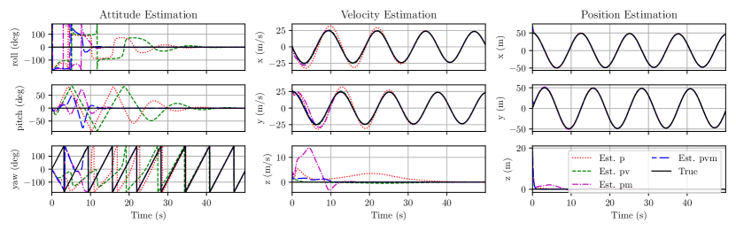
Figure 1: The estimated navigation states from the proposed observer using the four different sets of gains (p:$\cdots$, pv:- - -, pm:-$\cdot$-$\cdot$, pvm:— —) shown in Table 1 are shown along the true (—–) navigations states.

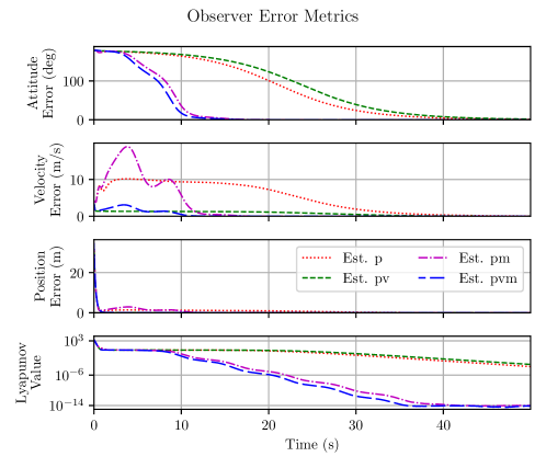
Figure 2: The errors in the estimated navigation states and the Lyapunov function value of the proposed observer using the four different sets of gains (p:$\cdots$, pv:- - -, pm:-$\cdot$-$\cdot$, pvm:— —) shown in Table 1.

Figure 1 shows the estimated navigation states obtained from the four observer variants along with the true states of the simulated system. Figure 2 shows the absolute errors in attitude, position, and velocity, in addition to the value of the Lyapunov function for each of the observers. One notes that the Lyapunov function is monotonically decreasing for each observer, which verifies Theorem 6.1. Additionally, each observer’s estimated states converge to the true states in spite of the extreme initial condition.

The advantage in using other measurements in addition to GNSS position is apparent in the convergence rates of the various states. Shown in the attitude estimation plots of Figure 1 and the attitude error plot of Figure 2, the yaw estimates of observers that utilise the magnetometer measurement (5) are seen to converge far more quickly than the observers that do not. Likewise, the velocity estimates of the observers that utilise the GNSS velocity measurement (4b) exhibit a far smaller initial error and converge more quickly than those of the observers that do not. It is interesting to compare the magnetometer ‘pm’ and velocity ‘pv’ observers: under the chosen simulation conditions, the ‘pm’ observer converges faster overall while the ‘pv’ observer incurs a much smaller initial error in both position and velocity. Understanding these behaviours can be useful for practitioners who may need to make tradeoffs between hardware based on typical operation scenarios.

What is perhaps surprising is that the attitude estimate of the ‘pv’ observer is slower to converge than the ‘p’ observer. This can be explained by the tradeoff between convergence of the position and velocity and damping of the persistence of excitation signal required to converge attitude when the magnetometer is not available. We believe that the behaviour of the ‘pv’ observer could be improved through more careful tuning of the gains, however, the gains here were chosen to be simple and similar across the observer designs to provide a demonstration of relative observer behaviour rather than tuned for a specific scenario.

8 Experiments

A real-world experiment was carried out using a remotely piloted aerial system (RPAS) equipped with the ArduPilot open source flight controller [29]. ArduPilot was used to record data from the IMU (350 Hz), magnetometer (10 Hz), and GNSS (5 Hz) over a period of six minutes while the plane flew around an area of approximately 400 m $\times$ 400 m. The GNSS measurements were converted from Latitude-Longitude-Altitude (LLA) into a local North-East-Down (NED) frame by using the first GNSS position measurement as a reference. The reference magnetic field was obtained from the ArduPilot Python tools as $\mathring{y}_{m}=(23.33,5.19,-52.80)$ $\mu$T. ArduPilot’s EKF3 is used for comparison with our proposed observer. It is based on a multiplicative Kalman filter [28] but also includes a range of initialisation and outlier rejection techniques to mitigate issues related to system nonlinearities and non-Gaussian measurement noise. The proposed observer was implemented at the rate of the IMU measurements, and the latest magnetometer and GNSS measurements were used as if they were current, i.e. the GNSS and magnetometer measurements were treated as piecewise constant in a zero-order hold scheme. The initial conditions were chosen as

$$\hat{R}(0) =I_{3}, \hat{v}(0) =0_{3\times 1}\text{~{}m/s}, \hat{p}(0) =0_{3\times 1}\text{~{}m},$$

$$\hat{R}_{Z}(0) =I_{3}, \hat{V}_{Z}(0) =0_{3\times 2}, \hat{A}_{Z}(0) =I_{2},$$

and the gains were set to

$$K_{q} =\operatorname{diag}(0.1,0.02), k_{p} =1.0, k_{c} =0.01,$$

$$k_{v} =1.0, k_{d} =0.001, k_{m} =2.0\times 10^{-6}.$$

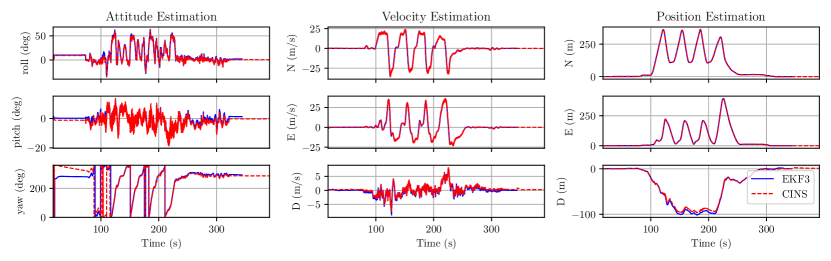
Figure 3: The estimated navigation states from the proposed observer (- - -) and the ArduPilot EKF3 (—–) over the whole experimental flight. The trajectory estimates are very similar.

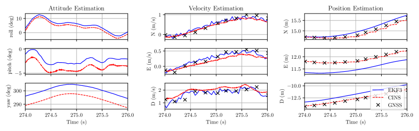
Figure 4: The estimated navigation states from the proposed observer (- - -) and the ArduPilot EKF3 (—–) and the GNSS measurements ($\times\times\times$) over a two second period of the experimental flight.

Figure 3 shows the navigation states estimated by the proposed observer compared with those provided by the ArduPilot EKF3 state estimator. Figure 4 additionally shows these estimates over two seconds alongside the GNSS measurements during this time. While the plane is stationary during the first 80 s of data, the yaw estimate of the proposed observer converges to be close to that provided by the EKF3. Throughout the flight, the estimated trajectories are very similar between the two observers, although there is a clear offset in the estimated heights (D-position). This is due to the EKF3 preferring the Barometer as a measurement of height over the GNSS, while the proposed observer only uses the GNSS. In the enlarged view presented in Figure 4, the effect of the zero-order hold scheme can be seen in the position estimates of the proposed observer. The effect is less pronounced in the velocity estimates, where it is interesting to note that the estimate provided by our proposed observer is significantly smoother than that provided by the EKF3. The discrepancy in attitude estimation is likely due to biases in the gyroscope and magnetometer measurements that are not considered in the proposed observer design. Compensating for such issues is left as an interesting open question for future work. Regardless, the proposed observer provides a solution for attitude, velocity, and position that is comparable to the state-of-the-art ArduPilot EKF3.

9 Conclusion

This paper proposes, to the authors’ knowledge, the first observer for INS with almost globally asymptotically and locally exponentially stable error dynamics. These properties are obtained by exploiting the newly recognised automorphism group $\mathbf{SIM}_{2}(3)$ of the extended special Euclidean group $\mathbf{SE}_{2}(3)$ and its application to developing a synchronous observer error. The resulting observer design is able to converge using only GNSS position measurements, or GNSS position with a combination of GNSS velocity and magnetometer measurements. A simulation is used to demonstrate the observer convergence of various gain configurations from an extreme initial condition with angle error of $0.99\pi$ rad, and a real-world experiment shows practical performance as compared to a state-of-the-art multiplicative EKF implementation.

This work opens a number of exciting avenues for future research. Including estimation of sensor biases into the present design is an important step for future practical implementations. The convergence of the attitude estimation could also perhaps be improved by exploring time-varying or non-scalar gains. Tightly coupled GNSS measurements have been shown to improve INS performance [15] and are also an interesting direction to consider. Overall, we hope that the design principles in this paper enable the development of further INS solutions with almost-global stability characteristics.

Appendix A Lemmas and Proofs

Lemma A.1.

Suppose that $R\in\mathbf{SO}(3)$ and $\dot{R}=-2kR(\hat{\mu}\times\mu)^{\times}$. If $\mu=R\hat{\mu}+\delta$, then

$$\frac{\mathrm{d}}{\mathrm{d}t}\operatorname{tr}(I_{3}-R)=-|(I_{3}-R^{2})\mu|^{2}-2k\langle(I_{3}-R^{2})\mu,\delta\rangle.$$

Proof.

Direct computation yields

$$\frac{\mathrm{d}}{\mathrm{d}t}\operatorname{tr}(I_{3}-R) =-\operatorname{tr}(\dot{R}),$$

$$=2\operatorname{tr}(kR(\hat{\mu}\times\mu)^{\times}),$$

$$=-2k\operatorname{tr}(R(\hat{\mu}\mu^{\top}-\mu\hat{\mu}^{\top})),$$

$$=-2k\operatorname{tr}(R\hat{\mu}\mu^{\top}-R\mu\hat{\mu}^{\top}),$$

$$=-2k\operatorname{tr}((\mu-\delta)\mu^{\top}-R\mu(R^{\top}\mu-R^{\top}\delta)^{\top}),$$

$$=-2k\operatorname{tr}(\mu\mu^{\top}-R\mu\mu^{\top}R-\delta\mu^{\top}+R\mu\delta^{\top}R),$$

$$=-2k\mu^{\top}(I_{3}-R^{2})\mu-k\mu^{\top}(I_{3}-R^{2})^{\top}\delta,$$

$$=-k\mu^{\top}(I_{3}-R^{2})^{\top}(I_{3}-R^{2})\mu$$

$$\hskip 28.45274pt-2k\mu^{\top}(I_{3}-R^{2})^{\top}\delta,$$

$$=-k|(I_{3}-R^{2})\mu|^{2}-2k\mu^{\top}(I_{3}-R^{2})^{\top}\delta.$$

This completes the proof. ∎

Proof of Lemma 5.2.

Direct computation in matrix form yields

$$\dot{Z} =(G+D)Z-Z\Gamma,$$

$$=\begin{pmatrix}0_{3\times 3}&W_{G}\\ 0_{2\times 3}&S_{D}\end{pmatrix}\begin{pmatrix}R_{Z}&V_{Z}\\ 0_{2\times 3}&A_{Z}\end{pmatrix}$$

$$\phantom{==}-\begin{pmatrix}R_{Z}&V_{Z}\\ 0_{2\times 3}&A_{Z}\end{pmatrix}\begin{pmatrix}\Omega_{\Gamma}^{\times}&W_{\Gamma}\\ 0_{2\times 3}&S_{\Gamma}\end{pmatrix},$$

$$=\begin{pmatrix}0_{3\times 3}&W_{G}A_{Z}\\ 0_{2\times 3}&S_{D}A_{Z}\end{pmatrix}-\begin{pmatrix}R_{Z}\Omega_{\Gamma}^{\times}&R_{Z}W_{\Gamma}+V_{Z}S_{\Gamma}\\ 0_{2\times 3}&A_{Z}S_{\Gamma}\end{pmatrix},$$

$$=\begin{pmatrix}-R_{Z}\Omega_{\Gamma}^{\times}&&&W_{G}A_{Z}-R_{Z}W_{\Gamma}-V_{Z}S_{\Gamma}\\ 0_{2\times 3}&&&S_{D}A_{Z}-A_{Z}S_{\Gamma}\end{pmatrix}.$$

∎

Proof of Lemma 5.3.

Expansion of (10) in matrix form yields

$$\bar{E} =\begin{pmatrix}R_{Z}&V_{Z}\\ 0_{2\times 3}&A_{Z}\end{pmatrix}^{-1}\begin{pmatrix}R&V\\ 0_{2\times 3}&I_{2}\end{pmatrix}\begin{pmatrix}\hat{R}&\hat{V}\\ 0_{2\times 3}&I_{2}\end{pmatrix}\begin{pmatrix}R_{Z}&V_{Z}\\ 0_{2\times 3}&A_{Z}\end{pmatrix},$$

$$=\begin{pmatrix}R_{Z}^{\top}&-R_{Z}^{\top}V_{Z}A_{Z}^{-1}\\ 0_{2\times 3}&A_{Z}^{-1}\end{pmatrix}\begin{pmatrix}R&V\\ 0_{2\times 3}&I_{2}\end{pmatrix}$$

$$\hskip 56.9055pt\begin{pmatrix}\hat{R}^{\top}&-\hat{R}^{\top}\hat{V}\\ 0_{2\times 3}&I_{2}\end{pmatrix}\begin{pmatrix}R_{Z}&V_{Z}\\ 0_{2\times 3}&A_{Z}\end{pmatrix},$$

$$=\begin{pmatrix}R_{Z}^{\top}R&-R_{Z}^{\top}V_{Z}A_{Z}^{-1}+R_{Z}^{\top}V\\ 0_{2\times 3}&A_{Z}^{-1}\end{pmatrix}$$

$$\hskip 56.9055pt\begin{pmatrix}\hat{R}^{\top}R_{Z}&\hat{R}^{\top}V_{Z}-\hat{R}^{\top}\hat{V}A_{Z}\\ 0_{2\times 3}&A_{Z}\end{pmatrix},$$

$$R_{\bar{E}} =R_{Z}^{\top}R\hat{R}^{\top}R_{Z},$$ (20)

$$V_{\bar{E}} =R_{Z}^{\top}R(\hat{R}^{\top}V_{Z}-\hat{R}^{\top}\hat{V}A_{Z})+(R_{Z}^{\top}V-R_{Z}^{\top}V_{Z}A_{Z}^{-1})A_{Z},$$

$$=R_{Z}^{\top}(VA_{Z}-V_{Z})-R_{\bar{E}}R_{Z}^{\top}(\hat{V}A_{Z}-V_{Z}).$$ (21)

Likewise, expansion of (11) in matrix form yields

$$\dot{\bar{E}} =\begin{pmatrix}\Omega_{\Gamma}^{\times}&W_{\Gamma}\\ 0_{2\times 3}&S_{\Gamma}\end{pmatrix}\begin{pmatrix}R_{\bar{E}}&V_{\bar{E}}\\ 0_{2\times 3}&I_{2}\end{pmatrix}-\begin{pmatrix}R_{\bar{E}}&V_{\bar{E}}\\ 0_{2\times 3}&I_{2}\end{pmatrix}\begin{pmatrix}\Omega_{\Gamma}^{\times}&W_{\Gamma}\\ 0_{2\times 3}&S_{\Gamma}\end{pmatrix}$$

$$\hskip 28.45274pt-\begin{pmatrix}R_{\bar{E}}&V_{\bar{E}}\\ 0_{2\times 3}&I_{2}\end{pmatrix}\begin{pmatrix}\Omega_{\Delta}^{\times}&W_{\Delta}\\ 0_{2\times 3}&0_{2\times 2}\end{pmatrix},$$

$$=\begin{pmatrix}\Omega_{\Gamma}^{\times}R_{\bar{E}}&\Omega_{\Gamma}^{\times}V_{\bar{E}}+W_{\Gamma}\\ 0_{2\times 3}&S_{\Gamma}\end{pmatrix}-\begin{pmatrix}R_{\bar{E}}\Omega_{\Gamma}^{\times}&R_{\bar{E}}W_{\Gamma}+V_{\bar{E}}S_{\Gamma}\\ 0_{2\times 3}&S_{\Gamma}\end{pmatrix}$$

$$\hskip 28.45274pt-\begin{pmatrix}R_{\bar{E}}\Omega_{\Delta}^{\times}&R_{\bar{E}}W_{\Delta}\\ 0_{2\times 3}&0_{2\times 2}\end{pmatrix},$$

$$\dot{R}_{\bar{E}} =\Omega_{\Gamma}^{\times}R_{\bar{E}}-R_{\bar{E}}(\Omega_{\Gamma}^{\times}+\Omega_{\Delta}^{\times}),$$ (22)

$$\dot{V}_{\bar{E}} =\Omega_{\Gamma}^{\times}V_{\bar{E}}-V_{\bar{E}}S_{\Gamma}+(I-R_{\bar{E}})W_{\Gamma}-R_{\bar{E}}W_{\Delta}.$$ (23)

This completes the proof. ∎

References

• [1] Martin Barczyk and Alan F. Lynch. Invariant Extended Kalman Filter design for a magnetometer-plus-GPS aided inertial navigation system. In 2011 50th IEEE Conference on Decision and Control and European Control Conference, pages 5389–5394, December 2011.
• [2] A. Barrau and S. Bonnabel. The Invariant Extended Kalman Filter as a Stable Observer. IEEE Transactions on Automatic Control, 62(4):1797–1812, April 2017.
• [3] Axel Barrau and Silvère Bonnabel. Invariant particle filtering with application to localization. In 53rd IEEE Conference on Decision and Control, pages 5599–5605, December 2014.
• [4] Soulaimane Berkane and Abdelhamid Tayebi. Position, Velocity, Attitude and Gyro-Bias Estimation from IMU and Position Information. In 2019 18th European Control Conference (ECC), pages 4028–4033, June 2019.
• [5] Soulaimane Berkane, Abdelhamid Tayebi, and Simone de Marco. A nonlinear navigation observer using IMU and generic position information. Automatica, 127:109513, May 2021.
• [6] S. Bonnabel, P. Martin, and E. Salaun. Invariant Extended Kalman Filter: Theory and application to a velocity-aided attitude estimation problem. In IEEE Conference on Decision and Control, pages 1297–1304, 2009.
• [7] Silvere Bonnabel. Left-invariant extended Kalman filter and attitude estimation. In Procedings of the IEEE Conference on Decision and Control (CDC), page 6 pages, New Orleans, LA, USA, 2007.
• [8] Fredrik Dukan and Asgeir J. Sørensen. Integration Filter for APS, DVL, IMU and Pressure Gauge for Underwater Vehicles. IFAC Proceedings Volumes, 46(33):280–285, January 2013.
• [9] Kevin Eckenhoff, Patrick Geneva, and Guoquan Huang. Closed-form preintegration methods for graph-based visual–inertial navigation. The International Journal of Robotics Research, 38(5):563–586, April 2019.
• [10] Michael George and Salah Sukkarieh. Tightly Coupled INS/GPS with Bias Estimation for UAV Applications. In Australasian Conference on Robotics and Automation, page 7, Sydney, Australia, December 2005.
• [11] Håvard Fjær Grip, Thor I. Fossen, Tor A. Johansen, and Ali Saberi. Nonlinear observer for GNSS-aided inertial navigation with quaternion-based attitude estimation. In 2013 American Control Conference, pages 272–279, June 2013.
• [12] Håvard Fjær Grip, Ali Saberi, and Tor A. Johansen. Observers for interconnected nonlinear and linear systems. Automatica, 48(7):1339–1346, July 2012.
• [13] Brian C. Hall. Lie Groups, Lie Algebras, and Representations: An Elementary Introduction, volume 222 of Graduate Texts in Mathematics. Springer International Publishing, Cham, 2015.
• [14] Jakob M. Hansen, Thor I. Fossen, and Tor Arne Johansen. Nonlinear observer design for GNSS-aided inertial navigation systems with time-delayed GNSS measurements. Control Engineering Practice, 60:39–50, March 2017.
• [15] Jakob M. Hansen, Tor Arne Johansen, Nadezda Sokolova, and Thor I. Fossen. Nonlinear Observer for Tightly Coupled Integrated Inertial Navigation Aided by RTK-GNSS Measurements. IEEE Transactions on Control Systems Technology, 27(3):1084–1099, May 2019.
• [16] John Henawy, Zhengguo Li, Wei Yun Yau, Gerald Seet, and Kong Wah Wan. Accurate IMU Preintegration Using Switched Linear Systems For Autonomous Systems. In 2019 IEEE Intelligent Transportation Systems Conference (ITSC), pages 3839–3844, October 2019.
• [17] Rui Hirokawa and Takuji Ebinuma. A Low-Cost Tightly Coupled GPS/INS for Small UAVs Augmented with Multiple GPS Antennas. NAVIGATION, 56(1):35–44, 2009.
• [18] Gerhard Paul Hochschild. The Structure of Lie Groups. Holden-Day, San Francisco, 1965.
• [19] Minh-Duc Hua. Attitude estimation for accelerated vehicles using GPS/INS measurements. Control Engineering Practice, 18(7):723–732, July 2010.
• [20] Minh-Duc Hua, Tarek Hamel, and Claude Samson. Riccati nonlinear observer for velocity-aided attitude estimation of accelerated vehicles using coupled velocity measurements. In 2017 IEEE 56th Annual Conference on Decision and Control (CDC), pages 2428–2433, December 2017.
• [21] Alireza Khosravian, Jochen Trumpf, Robert Mahony, and Tarek Hamel. State estimation for invariant systems on Lie groups with delayed output measurements. Automatica, 68:254–265, June 2016.
• [22] C. Lageman, J. Trumpf, and R. Mahony. Gradient-Like Observers for Invariant Dynamics on a Lie Group. IEEE Transactions on Automatic Control, 55(2):367–377, February 2010.
• [23] Y. Li, J. Wang, C. Rizos, P. Mumford, and W. Ding. Low-cost Tightly Coupled GPS/INS Integration Based on a Nonlinear Kalman Filtering Design. In Proceedings of the 2006 National Technical Meeting of The Institute of Navigation, pages 958–966, January 2006.
• [24] R. Mahony, T. Hamel, and J. Pflimlin. Nonlinear Complementary Filters on the Special Orthogonal Group. IEEE Transactions on Automatic Control, 53(5):1203–1218, June 2008.
• [25] Philippe Martin and Erwan Salaün. An Invariant Observer for Earth-Velocity-Aided Attitude Heading Reference Systems. IFAC Proceedings Volumes, 41(2):9857–9864, January 2008.
• [26] A. P. Morgan and K. S. Narendra. On the uniform asymptotic stability of certain linear nonautonomous differential equations. SIAM Journal on Control and Optimization, 15(1):5–24, 1977.
• [27] Andrew Roberts and Abdelhamid Tayebi. On the attitude estimation of accelerating rigid-bodies using GPS and IMU measurements. In 2011 50th IEEE Conference on Decision and Control and European Control Conference, pages 8088–8093, December 2011.
• [28] Joan Sola. Quaternion kinematics for the error-state Kalman filter. arXiv preprint arXiv:1711.02508, 2017.
• [29] Andrew Tridgell and Team. ArduPilot. https://ardupilot.org, 2010.
• [30] Jochen Trumpf, Robert Mahony, Tarek Hamel, and Christian Lageman. Analysis of Non-Linear Attitude Observers for Time-Varying Reference Measurements. IEEE Transactions on Automatic Control, 57(11):2789–2800, November 2012.
• [31] Pieter van Goor, Tarek Hamel, and Robert Mahony. Constructive Equivariant Observer Design for Inertial Navigation, August 2023.
• [32] Pieter van Goor, Tarek Hamel, and Robert Mahony. Constructive Equivariant Observer Design for Inertial Velocity-Aided Attitude. IFAC-PapersOnLine, 56(1):349–354, January 2023.
• [33] Pieter van Goor and Robert Mahony. Autonomous Error and Constructive Observer Design for Group Affine Systems. In 2021 60th IEEE Conference on Decision and Control (CDC), pages 4730–4737, December 2021.
• [34] B. Vik and T. Fossen. A nonlinear observer for GPS and INS integration. In Proceedings of the 40th IEEE Conference on Decision and Control, pages 2956–2961, 2001.
• [35] Miaomiao Wang and Abdelhamid Tayebi. A Globally Exponentially Stable Nonlinear Hybrid Observer for 3D Inertial Navigation. In 2018 IEEE Conference on Decision and Control (CDC), pages 1367–1372, December 2018.
• [36] Miaomiao Wang and Abdelhamid Tayebi. Observers Design for Inertial Navigation Systems: A Brief Tutorial. In 2020 59th IEEE Conference on Decision and Control (CDC), pages 1320–1327, December 2020.
• [37] Oliver J. Woodman. An introduction to inertial navigation. Technical Report UCAM-CL-TR-696, University of Cambridge, Computer Laboratory, 2007.