Active risk aversion in SIS epidemics on networks

Abstract

We present and analyze an actively controlled Susceptible-Infected-Susceptible (actSIS) model of interconnected populations to study how risk aversion strategies, such as social distancing, affect network epidemics. A population using a risk aversion strategy reduces its contact rate with other populations when it perceives an increase in infection risk. The network actSIS model relies on two distinct networks. One is a physical contact network that defines which populations come into contact with which other populations and thus how infection spreads. The other is a communication network, such as an online social network, that defines which populations observe the infection level of which other populations and thus how information spreads. We prove that the model, with these two networks and populations using risk aversion strategies, exhibits a transcritical bifurcation in which an endemic equilibrium emerges. For regular graphs, we prove that the endemic infection level is uniform across populations and reduced by the risk aversion strategy, relative to the network SIS endemic level. We show that when communication is sufficiently sparse, this initially stable equilibrium loses stability in a secondary bifurcation. Simulations show that a new stable solution emerges with nonuniform infection levels.

I Introduction

Infectious diseases are a persistent public health challenge. Compartmental models like SI, SIS, SIR, and SIRI offer mathematically tractable frameworks for understanding the spread of infection in populations - see [1, 2] for recent surveys. These models are useful in the design and evaluation of public health strategies for the containment and mitigation of infectious disease, such as the use of face masks in public, social distancing, partial lockdowns, and public vaccination strategies. The tractability of compartmental models makes them a compelling tool for analysis. However, they often do not account for human interactions and attitudes in the face of a disease, which can affect the spread of pathogens [3].

Various recent extensions to compartmental models on networks have been proposed to address these limitations. Typically, these extensions consider a second dynamic process that evolves alongside the infection spread, and in turn affects the infection spread dynamics. Several recent works study epidemics coupled with game-theoretic updates to self-protective strategies within populations, including factors such as fatigue and various economic and social costs [4, 5, 6, 7]. Other works couple epidemic and opinion dynamics [8, 9], and consider multi-layer networks [10, 11].

In this paper, we add to this literature and study SIS epidemic dynamics for networked populations that update their inter-population contact rate in response to a dynamic assessment of infection risk based on their possibly limited observations of infection level in other populations, e.g., from a social network. We focus on populations of risk averters that lower their contact rate with increased perceived infection risk.

The network SIS model of epidemics with state-dependent contact rates was recently studied in [12, 13, 14]. These works formulate distributed control laws to reduce endemic infection levels, with each population adjusting its contact rate in response to its own infection level. In contrast, we focus on the impact of risk perception on infection levels when populations can observe infection levels of other populations.

We propose and study network actSIS (actively controlled Susceptible-Infected-Susceptible), a reactive model for networked populations. The model relies on two networks: 1) a contact network that defines which populations come into contact with which other populations and thus how infection spreads and 2) a communication network that defines which populations observe the infection level of which other populations and thus how information spreads. We examine the effect of risk aversion and the two network structures on epidemic spread. A notion of risk perception was studied in epidemics in [4, 5]; however, the analysis uses a mean-field limit, which does not reveal the role of network structure.

Our main contributions are as follows. First, we extend actSIS, a well-mixed population model of actively controlled SIS epidemics, introduced in [15], to network actSIS, a model of interconnected populations, with a contact network that governs infection spread and communication network that governs risk assessment. Second, for this model we prove the emergence of an endemic equilibrium (EE) in a transcritical bifurcation. On regular graphs, we prove that risk aversion lowers the (uniform) infection levels at this EE. Third, we show that an EE in this model is not necessarily unique; it can lose stability in a secondary bifurcation if the communication network is sufficiently sparse. On regular communication and influence graphs, stability loss leads to emergence of an infection state that is heterogeneous, i.e., nonuniform infection levels, despite a high level of homogeneity in model structure and parameters.

In Section II we provide mathematical preliminaries and background on SIS models. In Section III we introduce the network actSIS model. We analyze the model with general graphs and risk response strategies in Section IV and specialized to regular graphs in Section V.

II Background

II-A Notation and preliminaries

Given a vector $\mathbf{x}\in\mathbb{R}^{n}$, $\text{diag}(\mathbf{x})$ is the matrix with diagonal entries $x_{i}$, and zero off-diagonal entries. Given two vectors $\mathbf{x},\mathbf{y}\in\mathbb{R}^{n}$, we say $\mathbf{x}\succ\mathbf{y}$ if $x_{j}>y_{j}$, and $x\succeq y$ if $x_{j}\geq y_{j}$ for all $j\in\{1,\ldots,n\}$, with similar element-wise definitions for matrices. We denote by 0 and 1 the vectors of appropriate dimension whose entries are all equal to $0$ and $1$, respectively. A matrix is reducible if it is similar to an upper-triangular matrix, and it is irreducible if it is not reducible. A square matrix $A$ is Metzler if its off-diagonal entries are nonnegative. More precisely, $a_{ij}\geq 0$ for all $i\neq j$. Given a square matrix $A$, let $\{\lambda_{i}\}$ be the set of eigenvalues of $A$, the spectral radius of $A$ is $\rho(A)=\max\{|\lambda_{i}|:i\in\{1,\ldots,n\}\}$. A leading eigenvalue of $A$ is $\lambda_{max}(A)=\operatorname{argmax}\{\operatorname{Re}(\lambda_{i})\}$. $A$ is Hurwitz if $\operatorname{Re}(\lambda_{max}(A))<0$. If $A$ is a Metzler, irreducible matrix, then $\rho(A)>0$ is a simple leading eigenvalue of $A$ with associated left and right eigenvectors $\mathbf{w}\succ\mathbf{0}$, $\mathbf{v}\succ\mathbf{0}$. For nonnegative $A$ this is the classic Perron-Frobenius property and $\mathbf{w},\mathbf{v}$ are the Perron-Frobenius eigenvectors. The decomposition $A=T+U$ for a Metzler matrix $A$ is a regular splitting if $U$ is Hurwitz and Metzler, and $T\succeq 0$. For a Metzler $A$ with regular splitting $T+U$, $\lambda_{max}(A)>0(=0)$ if and only if $\rho(TU^{-1})>0(=0)$ [16].

A graph $\mathcal{G}=(\mathcal{V},\mathcal{E})$ is a collection of $n$ nodes $\mathcal{V}$ and edges $\mathcal{E}$. Node $j\in\mathcal{V}$ is a neighbor of node $i\in\mathcal{V}$ on the graph $\mathcal{G}$ whenever the edge $(i,j)\in\mathcal{E}$. The adjacency matrix $A$ encodes relationships on graph $\mathcal{G}$, with $(A)_{ij}=1$ whenever $(i,j)\in\mathcal{E}$ and $0$ otherwise. A graph is undirected whenever $(i,j)\in\mathcal{E}$ if and only if $(j,i)\in\mathcal{E}$, i.e. $A=A^{T}$; it is directed otherwise. The in-degree of a node $j\in\mathcal{V}$ is $d_{j}=\sum_{k=1}^{N}a_{jk}$. We say a graph is regular with in-degree $d$ if $d_{j}=d$ for all $j\in\mathcal{V}$. A graph is strongly connected if, for all pairs of vertices $i,j$, there is a path from $i$ to $j$. We know that a graph $\mathcal{G}$ is strongly connected if and only if $A$ is irreducible. In this paper we primarily reference graphs by referencing their associated adjacency matrix.

II-B SIS and actSIS models

The Susceptible-Infected-Susceptible (SIS) model describes the spread of infection in a population of agents as

$$\dot{p}=\beta(1-p)p-\delta p,$$ (1)

where $p\in[0,1]$ is the proportion of the population that is currently infected, $\delta>0$ is the recovery rate, and $\beta>0$ is the rate of infection transmission. The network SIS model generalizes the traditional SIS model by incorporating structured contact patterns among a set of populations through interactions over a contact network. Each node in the contact network graph signifies a separate population, and edges encode whether these populations come into contact. The infection level $p_{j}\in[0,1]$ in population $j$ evolves as

$$\dot{p}_{j}=\left(1-p_{j}\right)\beta\sum_{k=1}^{N}a_{jk}p_{k}-\delta p_{j}.$$ (2)

$\beta$ and $\delta$ are infection and recovery rates. $a_{jk}=a_{kj}=1$ if populations $j$ and $k$ comes into contact and $0$ otherwise.

While traditional SIS models consider $\beta$ to be a fixed parameter, in reality, populations can dynamically adapt their contact behavior, for example by practicing social distancing or by avoiding public places when infection levels rise. To account for this, the Actively Controlled SIS (actSIS) model, introduced in [15], extends the traditional SIS framework by incorporating adaptive contact rates based on perceived infection risk. The model features two variables: the actual infection rate $p\in[0,1]$, and a filtered observation $p_{s}\in[0,1]$ that represents the perceived infection level on which the population bases its risk assessment. The effective infection rate can be expressed as $\beta(p_{s})=\bar{\beta}\alpha(p_{s})$ where $\bar{\beta}$ is the intrinsic transmission rate of the disease and $\alpha:[0,1]\to[0,1]$ models the contact rate which actively adapts to perceived risk. The variables co-evolve according to

$$\dot{p} =\bar{\beta}\alpha(p_{s})(1-p)p-\delta p,$$ (3)

$$\tau_{s}\dot{p}_{s} =-p_{s}+p,$$ (4)

where $\tau_{s}$ is a time constant that captures a potential delay in the transmission of information about infection levels.

III Network actSIS Model

To study the effect of adaptive contact rates on the infection levels in interconnected populations, we extend the actSIS model from its original well-mixed statement (3),(4) to network actSIS, which incorporates network interactions. Analogously to the classic network SIS model, for the network actSIS model, we let $p_{j}\in[0,1]$ be the infection level of population $j$, and define a contact graph with adjacency matrix $A=(a_{ij})$. We introduce $p_{sj}\in[0,1]$ as the perceived global infection level within population $j$, and we define the communication graph with adjacency matrix $\hat{A}=(\hat{a}_{jk})$. The contact graph is associated with the spread of infection, whereas the communication graph encodes which populations influence the perception of risk of which others. The two graphs can be the same, or may differ, for example with $A$ representing physical contact between populations and $\hat{A}$ representing interactions in an online social network.

For each population $j$, the effective contact rate with neighboring populations is $\beta_{j}(p_{s})=\bar{\beta}\alpha_{j}(p_{s})$ where $\bar{\beta}$ is the intrinsic transmission rate and $\alpha_{j}:[0,1]\to[0,1]$ models the response to risk of population $j$. This formulation allows for potentially heterogeneous risk response strategies on the network. We assume each $\alpha_{j}$ is continuously differentiable on the unit interval (i.e. $C^{1}$), $|\alpha_{j}^{\prime}(p_{s})|<\infty$ for any $p_{s}\in[0,1]$, and $\alpha_{j}(0)\neq 0$ for all $j\in\mathcal{V}$. The infection level within population $j$ and its filtered observation of infection among its neighbors co-evolve according to

$$\dot{p}_{j} =\left(1-p_{j}\right)\bar{\beta}\alpha_{j}(p_{sj})\sum_{k=1}^{N}a_{jk}p_{k}-\delta_{j}p_{j},$$ (5)

$$\tau_{s}\dot{p}_{sj} =-p_{sj}+\frac{1}{\hat{d}_{j}}\left(\sum_{k=1}^{N}\hat{a}_{jk}p_{k}\right)$$ (6)

where $\hat{d}_{j}=:\sum_{k=1}^{N}\hat{a}_{jk}$ is the in-degree of node $j$ on the communication graph associated to $\hat{A}$.

IV Theoretical results for general model

In this section, we present an analysis of the network actSIS model (5), (6). First, we establish that the model is well-posed, in the sense that the infection rate $p_{j}$ and perceived global infection rate $p_{sj}$ for each population $j\in\mathcal{V}$ remain within the interpretable set $[0,1]\subset\mathbb{R}$.

Theorem IV.1 (Well-Definedness).

The set $\mathcal{S}=[0,1]^{2N}$ is forward invariant for the network actSIS dynamics (5),(6).

Proof.

To prove this statement we invoke Nagumo’s theorem [17, Theorem 4.7]. The boundary of $\mathcal{S}$ is the set $\partial\mathcal{S}$ of all points at which $p_{j}=0$, $p_{j}=1$, $p_{sj}=0$, and/or $p_{sj}=1$ for one or more $j\in\mathcal{V}$. Observe that whenever $(\boldsymbol{p},\boldsymbol{p}_{s})\in\partial\mathcal{S}$, $p_{j}=0\implies\dot{p}_{j}=\bar{\beta}\sum_{k=1}^{N}\alpha_{jk}(p_{sj})p_{k}\geq 0$; $p_{j}=1\implies\dot{p}_{j}=-\delta_{j}<0$; $p_{sj}=0\implies\dot{p}_{sj}=\frac{1}{\tau_{s}\hat{d}_{j}}\sum_{k=1}^{N}\hat{a}_{jk}p_{k}\geq 0$; and $p_{sj}=1\implies\dot{p}_{sj}=(-1+\frac{1}{\hat{d}_{j}}\sum_{k=1}^{N}\hat{a}_{jk}p_{k})/\tau_{sj}\leq 0$ for all $j\in\mathcal{V}$. Therefore at every point on the boundary $\partial\mathcal{S}$, the vector field of the dynamics points along the tangent cone $\mathcal{T}_{\mathcal{S}}(\boldsymbol{p},\boldsymbol{p}_{s})$. Compactness of $\mathcal{S}$ implies existence and uniqueness of solutions of (5),(6), in $\mathcal{S}$ for all $t\geq 0$ [18, Theorem 3.3], from which the theorem statement follows by [17, Corollary 4.8]. ∎

Next, we investigate the existence and stability of equilibria in the model. The Jacobian of the linearization of (5),(6) about an arbitrary point $(\mathbf{p},\mathbf{p}_{s})\in[0,1]^{2N}$ is

$$J(\mathbf{p},\mathbf{p}_{s})=\begin{pmatrix}-D+\bar{\beta}F_{1}(P_{1}A-P_{2})&\bar{\beta}F_{2}P_{1}P_{2}\\ \frac{1}{\tau_{s}}\hat{\Delta}^{-1}\hat{A}&-\frac{1}{\tau_{s}}I\end{pmatrix}$$ (7)

where $D=\operatorname{diag}\{(\delta_{1},\dots,\delta_{N})\}$, $P_{1}=\operatorname{diag}\{\mathbf{1}-\mathbf{p}\}$, $P_{2}=\operatorname{diag}\{A\mathbf{p}\}$, $F_{1}=\operatorname{diag}\{\alpha_{1}(p_{s1}),\dots,\alpha_{N}(p_{sN})\}$, $F_{2}=\operatorname{diag}\{(\alpha_{1}^{\prime}(p_{s1}),\dots,\alpha_{N}^{\prime}(p_{sN}))\}$. Observe that the infection-free state $(\mathbf{p},\mathbf{p}_{s})=(\mathbf{0},\mathbf{0})$ is always an equilibrium of (5), (6). At this equilibrium, (7) simplifies to

$$J_{IFE}=\begin{pmatrix}-D+\bar{\beta}\operatorname{diag}\{\alpha_{1}(0),\dots,\alpha_{N}(0)\}A&0\\ \frac{1}{\tau_{s}}\hat{\Delta}^{-1}\hat{A}&-\frac{1}{\tau_{s}}I\end{pmatrix}.$$ (8)

In the following theorem, we establish a transcritical bifurcation of the origin in the network actSIS model, in which the infection-free equilibrium (IFE) loses stability, and a stable endemic equilibrium (EE) appears.

Theorem IV.2 (Local bifurcation of EE).

Consider (5),(6), assume $A$, $\hat{A}$ are irreducible, define $\tilde{A}=\operatorname{diag}\{(\alpha_{1}(0),\dots,\alpha_{N}(0)\}A$. Then following statements hold. 1) The IFE is locally exponentially stable for $\bar{\beta}<\bar{\beta}^{*}=\frac{1}{\rho(\tilde{A}D^{-1})}$, and unstable for $\bar{\beta}>\bar{\beta}^{*}.$ 2) Let $\mathbf{v}^{*}\succ\mathbf{0}$, $\mathbf{w}^{*}\succ\mathbf{0}$ be right and left null eigenvectors of $-D+\bar{\beta}^{*}\tilde{A}$, and suppose

$$K_{1}=\sum_{i=1}^{N}w_{i}^{*}\left((\hat{\Delta}^{-1}\hat{A}\mathbf{v}^{*})_{i}\alpha_{i}^{\prime}(0)(A\mathbf{v}^{*})_{i}-2v_{i}^{*}\alpha_{i}(0)(A\mathbf{v}^{*})_{i}\right)$$

If $K_{1}\neq 0$, at $\bar{\beta}=\bar{\beta}^{*}$, a branch of locally exponentially stable EE, $\boldsymbol{p}^{*}\succ\mathbf{0}$, $\boldsymbol{p}_{s}^{*}=\hat{\Delta}^{-1}\hat{A}\boldsymbol{p}^{*}\succeq\mathbf{0}$, appear in a transcritical bifurcation along an invariant center manifold tangent to $\operatorname{span}(\bar{\mathbf{v}})$ at $(\mathbf{p},\mathbf{p}_{s},\bar{\beta})=(\mathbf{0},\mathbf{0},\bar{\beta}^{*})$, where $\bar{\mathbf{v}}=(\mathbf{v}^{*},\hat{\Delta}^{-1}\hat{A}\mathbf{v}^{*})$. If $K_{1}<0$, the EE appear for $\bar{\beta}>\bar{\beta}^{*}$ and are locally exponentially stable; if $K_{1}>0$, the EE appear for $\bar{\beta}<0$ and are unstable.

Proof.

1) Observe that $J_{IFE}$ (8) is block diagonal. The bottom block has eigenvalues $-1/\tau_{s}$ with multiplicity $N$ that are always negative, and the top block is the matrix $-D+\bar{\beta}\tilde{A}$. It is an irreducible Metzler matrix by assumptions of the theorem, and therefore has a unique eigenvalue $\lambda_{max}(-D+\bar{\beta}\tilde{A})$ that is negative if and only if $\bar{\beta}\rho(\tilde{A}D^{-1})<1$ and zero if and only if $\bar{\beta}\rho(\tilde{A}D^{-1})=1$, with corresponding positive eigenvector $\mathbf{v}^{*}(\bar{\beta})$. Therefore, when $\bar{\beta}<\bar{\beta}^{*}$, all of the eigenvalues of (8) are negative and the IFE is locally exponentially stable. When $\bar{\beta}>\bar{\beta}^{*}$, the IFE is unstable [18, Theorem 4.7]. 2) When $\bar{\beta}=\bar{\beta}^{*}$, $J_{IFE}$ has a zero eigenvalue; existence of an attracting invariant center manifold of the IFE follows by the Center Manifold Theorem [19, Theorem 3.2.1]. To classify the bifurcation we utilize results from singularity theory of bifurcations [20] and compute a Lyapunov-Schmidt (LS) reduction expansion. A LS reduction is a low-dimensional algebraic equation that describes the local topology of the bifurcation diagram (its solution sets are in one-to-one correspondence with the zero level sets of (5),(6) near $\bar{\beta}^{*}$). A second order LS reduction for (5),(6) reads $h(x,\bar{\beta})=K_{0}x(\bar{\beta}-\bar{\beta}^{*})+\bar{\beta}^{*}K_{1}x^{2}+h.o.t.$ where $x$ is a scalar coordinate along a projection of the dynamics onto the kernel of $J_{IFE}$ at $\bar{\beta}=\bar{\beta}^{*}$ and $K_{0}=\langle\mathbf{w}^{*},\tilde{A}\mathbf{v}^{*}\rangle>0$. The details of this calculation are included in the Appendix. To identify the transcritical bifurcation, we verify that the LS reduction coefficients satisfy the necessary and sufficient conditions of the recognition problem [20, Proposition 9.3]: $h(0,\bar{\beta}^{*})=h_{x}(0,\bar{\beta}^{*})=h_{\beta}(0,\bar{\beta}^{*})=0$ where $\beta=\bar{\beta}-\bar{\beta}^{*}$. Furthermore, $\operatorname{sign}\{h_{xx}(0)\}=\operatorname{sign}(K_{1})$ and $\operatorname{sign}\{\det d^{2}h(0)\}=-1$, where

$$\det d^{2}h(0)=\begin{vmatrix}h_{xx}(0)&h_{x\beta}(0)\\ h_{x\beta}(0)&h_{\beta\beta}(0)\end{vmatrix}=\begin{vmatrix}\bar{\beta}^{*}K_{1}&K_{0}\\ K_{0}&0\end{vmatrix}=-(K_{0})^{2}.$$

The conditions are verified, and we conclude that the bifurcation is a transcritical bifurcation of equilibria. Local stability of the bifurcating branch of endemic equilibria follows by [20, Chapter I, §4, Theorem 4.1]. ∎

Corollary IV.1.

Consider (5),(6). 1) If $\alpha_{j}^{\prime}(0)\leq 0$ for all $j\in\mathcal{V}$, then $K_{1}<0$ and locally exponentially stable EE appear for $\bar{\beta}>\bar{\beta}^{*}$; 2) If $\delta_{j}=\delta>0$, $\alpha_{j}(0)=1$ for all $j\in\mathcal{V}$, then $\bar{\beta}^{*}=\delta/\lambda_{max}(A)$ and $\mathbf{v}^{*}\succ\mathbf{0}$ is a Perron-Frobenius eigenvector of $A$.

Case 1 of Corollary IV.1 is relevant in the next section where we study networks of risk averter populations. Case 2 shows mild conditions under which the critical value $\bar{\beta}*$ is directly related to the leading eigenvector of unweighted contact matrix $A$ and the EE infection levels are predicted by the elements of the Perron-Frobenius eigenvector of $A$.

According to Theorem IV.2, the IFE in the network actSIS model (5),(6) loses stability in a transcritical bifurcation. This result is an extension of a similar transcritical bifurcation of an EE that is well-known to exist in the SIS, network SIS, and more recently actSIS models [1], [15]. Interestingly, the communication adjacency matrix $\hat{A}$ does not determine the bifurcation point of the EE and does not play a significant role in shaping the steady-state infection level at the EE near the bifurcation point. However, recall that in the network SIS model, the EE is unique and stable for all $\bar{\beta}>\bar{\beta}^{*}$. We will show in the following section that this is not always the case for the EE of Theorem IV.2, and properties of this equilibrium at larger values of $\bar{\beta}$ depend strongly on properties of the communication graph $\hat{A}$.

V Risk aversion in network actSIS epidemics

In this section, we specialize the network actSIS model (5),(6) to populations of risk averters. We say population $j$ is following a risk aversion strategy if it decreases its contact rate with other populations when its perceived risk of infection rises, i.e. $\alpha_{j}^{\prime}(p_{sj})<0$ whenever $p_{sj}\in(0,1)$. For all simulations, we assume all populations are following the same strategy $\alpha_{A}$, proposed in [15], described by the saturating function

$$\alpha_{j}(p_{sj})=\alpha_{A}(p_{sj}):=\frac{\mu^{\nu}(1-p_{sj})^{\nu}}{p_{sj}^{\nu}(1-\mu)^{\nu}+\mu^{\nu}(1-p_{sj})^{\nu}}$$ (9)

where $\mu\in(0,1)$ is a parameter that describes the midpoint of saturation, and $\nu>1$ is a parameter related to the maximal steepness of the slope. First we establish a lemma for the well-mixed actSIS model (3),(4).

Lemma V.1 (Risk aversion lowers EE in well-mixed model).

Consider the well-mixed SIS (1) and actSIS (3),(4) models with $\beta=\bar{\beta}>\delta$ and $\alpha^{\prime}(p)<0$ for all $p\in(0,1)$. Let $p^{*}_{\text{SIS}}(\bar{\beta},\delta)$ and $p^{*}_{\text{actSIS}}(\bar{\beta},\delta)$ be the steady-state infection level in the population at the EE of the corresponding model, with shared $\delta$, $\bar{\beta}>\bar{\beta}^{*}$. If $\alpha$ is a risk aversion strategy, then $p^{*}_{\text{SIS}}(\bar{\beta},\delta)\geq p^{*}_{\text{actSIS}}(\bar{\beta},\delta)$.

Proof.

Define the function $\gamma(p,s):=(1-s)+s\alpha(p)$ with $s\in[0,1]$, and consider (3),(4) with $\alpha$ replaced by $\gamma$. Notice that $s=0$ recovers the standard SIS model (1), and $s=1$ recovers the actSIS model (3),(4). The equilibria of this modified model are defined implicitly as a function of $s$ by $\bar{\beta}\gamma(p^{*},s)(1-p^{*})p^{*}-\delta p^{*}=0$ and $p_{s}^{*}=p^{*}$. Differentiating this with respect to $s$ and solving for $\frac{dp^{*}}{ds}$ we obtain

$$\frac{dp^{*}}{ds}=\frac{(1-p^{*})(1-\alpha(p^{*}))}{s\big{(}\alpha^{\prime}(p^{*})(1-p^{*})+(1-\alpha(p^{*}))\big{)}-1}.$$ (10)

For any $p^{*}\in(0,1)$, $\alpha(p^{*})\in(0,1)$ and the numerator in (10) is positive. Observe that whenever $\alpha^{\prime}(p^{*})<\frac{1/s-(1-\alpha)}{1-p^{*}}$ the denominator of (10) is negative and $\frac{dp^{*}}{ds}<0$. Given any $s\in(0,1)$, $1<1/s<\infty$, which means that $\alpha^{\prime}(p^{*})<\frac{\alpha(p^{*})}{1-p^{*}}$ is sufficient to conclude $\frac{dp^{*}}{ds}<0$. In turn, this condition is satisfied for all $p^{*}\in(0,1)$ given any $\alpha$ satisfying assumptions of the Lemma, since $\alpha(p^{*})/(1-p^{*})>0$, and $\alpha^{\prime}(p)<0$ by definition of risk aversion. ∎

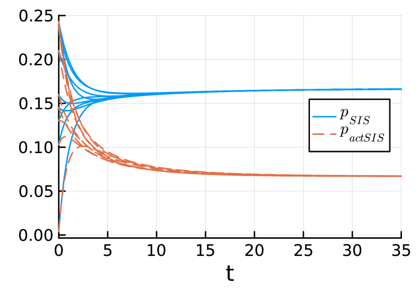
(a) $\deg(A)=2$ and $\deg(\hat{A})=5$.

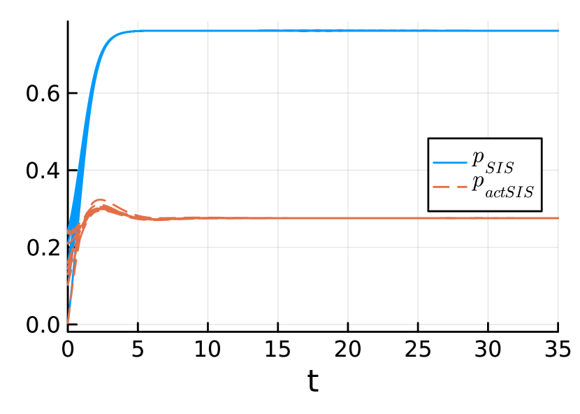
(b) $\deg(A)=7$ and $\deg(\hat{A})=5$.

Figure 1: Simulation for network actSIS (5),(6) with $10$ nodes and regular contact graph and communication graph, using [21]. The degree of $\hat{A}$ is constant but $A$ is sparse (left) or dense (right). Parameters: $\bar{\beta}=0.3,\delta=0.5,\mu=0.5,\nu=1.7,\tau_{s}=1$.

Lemma V.1 formalizes the observation that risk aversion lowers infection rate at endemic equilibrium in (3),(4), originally made in numerical experiments in [15]. Next, we consider risk aversion strategies in network actSIS, and prove an analogous result. We restrict our attention to contact and communication graphs that are undirected and regular. By Corollary IV.1, for populations of risk averters, the necessary and sufficient conditions for a transcritical bifurcation of a stable endemic equilibrium in Theorem IV.2 are always satisfied.

Lemma V.2 (Uniform Endemic Equilibrium (UEE)).

Let $A$ and $\hat{A}$ correspond to connected regular graphs with degrees $d$ and $\hat{d}$, respectively, and assume $\delta_{j}=\delta$, $\alpha_{j}=\alpha$ for all $j\in\mathcal{V}$. 1) The unique, globally stable EE of the network SIS model (2) with contact graph $A$ is $\mathbf{p}^{*}_{SIS}=p_{SIS}^{*}\mathbf{1}$ where $p_{SIS}^{*}=1-\frac{\delta}{\bar{\beta}d}$; 2) The EE bifurcating from IFE for the network actSIS model (5),(6) with contact graph $A$ and communication graph $\hat{A}$ is $(\mathbf{p}_{actSIS}^{*},\mathbf{p}_{s}^{*})=(p_{actSIS}^{*}\mathbf{1},p_{actSIS}^{*}\mathbf{1})$ where $p_{actSIS}^{*}$ is implicitly defined through $\bar{\beta}d(1-p_{actSIS}^{*})\alpha(p_{actSIS}^{*})-\delta=0$. Furthermore, this equilibrium exists for all $\bar{\beta}>\delta/d$.

Lemma V.2 says that the EE (that bifurcates from the IFE) for regular graphs corresponds to uniform levels of infection among the populations in network SIS and network actSIS. We omit the proof of Lemma V.2 as it amounts to plugging in the stated expressions into the two sets of model equations.

Theorem V.3 (Risk aversion lowers UEE on regular graphs).

Let $A$ and $\hat{A}$ correspond to connected regular graphs with degrees $d$ and $\hat{d}$, respectively, and assume $\delta_{j}=\delta$, $\alpha_{j}=\alpha$ for all $j\in\mathcal{V}$, and $\alpha^{\prime}(p)<0$ for all $p\in(0,1)$. Let $\mathbf{p}^{*}_{SIS}$ be the UEE of (2) with $\beta=\bar{\beta}>\delta/d$, and let $(\mathbf{p}_{actSIS}^{*},\mathbf{p}_{s}^{*})$ be the UEE of (5),(6). Then $\mathbf{p}_{SIS}^{*}\succeq\mathbf{p}^{*}_{actSIS}$.

Proof.

Existence of UEE in both models for $\bar{\beta}\geq\delta/d$ follows from Lemma V.2. It remains to show that $p_{SIS}^{*}\geq p_{actSIS}^{*}$. Defining the function $\gamma(p,s):=(1-s)+s\alpha(p)$ with $s\in[0,1]$, note that the solution to$\bar{\beta}d\gamma(p^{*},s)(1-p^{*})-\delta=0$ recovers $p_{SIS}^{*}$ when $s=0$ and $p_{actSIS}^{*}$ when $s=1$. The rest of the proof follows identically to Lemma V.1. ∎

We illustrate Theorem V.3 with numerical simulations in Figure 1. As predicted, the infection level at the UEE is uniform among populations and lower for the network actSIS dynamics than for the network SIS dynamics, with all other relevant parameters shared between the models.

Theorem V.4 (Stability of UEE on regular graphs).

Consider (5),(6). Let $A$ and $\hat{A}$ correspond to connected regular graphs with degrees $d$ and $\hat{d}$, respectively, and assume $\delta_{j}=\delta$, $\alpha_{j}=\alpha$ for all $j\in\mathcal{V}$. Define

$$g(p)=-\delta p+(1-p)\left(\lambda_{max}\left(\frac{1}{d}A+\frac{1}{\hat{d}}\frac{\alpha^{\prime}(p)}{\alpha(p)}p\hat{A}\right)-1\right)\,.$$ (11)

If $g(p)=0$ for some $p\in(0,1)$, then there exists a critical value $\bar{\beta}_{2}=\frac{\delta}{d(1-p_{2})\alpha(p_{2})}>\bar{\beta}^{*}$ where $p_{2}$ is the smallest $p\in(0,1)$ for which $g(p)=0$. If $p_{2}$ is not a unique solution to $g(p)=0$ in $(0,1)$, the UEE $(\mathbf{p}^{*},\mathbf{p}_{s}^{*})=(p^{*}\mathbf{1},p^{*}\mathbf{1})$ is locally exponentially stable whenever $\bar{\beta}^{*}<\bar{\beta}<\bar{\beta}_{2}$ and unstable for $\bar{\beta}\in(\bar{\beta}_{2},\bar{\beta}_{3})$ for some $\bar{\beta}_{3}=\frac{\delta}{d(1-p_{3})\alpha(p_{3})}$, $p_{3}>p_{2}$, $g(p_{3})=0$. If $p_{2}$ is a unique solution to $g(p)=0$ in $(0,1)$, then the UEE is unstable for all $\bar{\beta}>\bar{\beta}_{2}$.

Proof.

Existence of the uniform endemic equilibrium for $\bar{\beta}>\bar{\beta}^{*}$ was established in Theorem V.3, and its local exponential stability at the onset of the transcritical bifurcation follows from Theorem IV.2. From the form of the Jacobian matrix (7) we infer that its eigenvalues are continuous in the parameter $\bar{\beta}$, which means that the UEE is locally exponentially stable until one or more eigenvalues of $J(\mathbf{p}^{*},\mathbf{p}_{s}^{*})$ are singular for some $\bar{\beta}>\bar{\beta}^{*}$. At $(p^{*}\mathbf{1},p^{*}\mathbf{1})$, (7) simplifies to

$$J_{U}(p^{*})=\begin{pmatrix}-\delta\left(1+\bar{\beta}dp^{*}\alpha(p^{*})\right)I+\frac{\delta}{d}A&\delta\frac{\alpha^{\prime}(p^{*})}{\alpha(p^{*})}p^{*}I\\ \frac{1}{\tau_{s}}\frac{1}{\hat{d}}\hat{A}&-\frac{1}{\tau_{s}}I\end{pmatrix}$$ (12)

where we used $\bar{\beta}(1-p^{*})\alpha(p^{*})d=\delta$ to eliminate terms. Using Schur’s formula [22, Theorem 2.1],

$$\det(J_{U}(p^{*})-\lambda I)=\det\left(-\left(\frac{1}{\tau_{s}}+\lambda\right)I\right)\\ \times\det\left(-(\delta\left(1+\bar{\beta}dp^{*}\alpha(p^{*})\right)+\lambda)I+\frac{\delta}{d}A+\frac{\delta}{\hat{d}}\frac{\alpha^{\prime}(p^{*})}{\alpha(p^{*})}p^{*}\hat{A}\right)$$

which, noting that $p^{*}$ is an implicit function of $\bar{\beta}$, means that eigenvalues of $J_{U}(p^{*})$ that have a dependence on $\bar{\beta}$ are eigenvalues of the matrix

$$J_{eff}(p^{*})=-\delta\left(1+\bar{\beta}dp^{*}\alpha(p^{*})\right)I+\frac{\delta}{d}A+\frac{\delta}{\hat{d}}\frac{\alpha^{\prime}(p^{*})}{\alpha(p^{*})}p^{*}\hat{A}.$$ (13)

Each eigenvalue of (13) takes the form $\lambda_{i}(J_{eff}(p^{*}))=-\delta\left(1+\bar{\beta}dp^{*}\alpha(p^{*})\right)+\delta\lambda_{i}(M(p^{*}))$ where $M(p^{*})=\frac{1}{d}A+\frac{1}{\hat{d}}\frac{\alpha^{\prime}(p^{*})}{\alpha(p^{*})}p^{*}\hat{A}$. We are interested in the case that the largest eigenvalue $\lambda_{max}(J_{eff}(p^{*}))=0$, as it corresponds to the uniform equilibrium changing stability. At a singular point,

$$\bar{\beta}=\frac{1}{dp^{*}\alpha(p^{*})}(-1+\lambda_{max}(M(p^{*})))=\frac{\delta}{(1-p^{*})d\alpha(p^{*})}$$

where the first expression is derived from the zero eigenvalue condition and the second is from the equilibrium condition. Algebraic manipulations of the above statement lead to the condition $g(p)=0$. Finally, notice that $\lambda_{max}(J_{eff}(p^{*}))=\delta g(p^{*})/(1-p^{*})$ which means $\operatorname{sign}(\lambda_{max}(J_{eff}(p^{*})))=\operatorname{sign}(g(p^{*}))$. Local stability of the UEE can thus be inferred from the sign of $g(p^{*})$ and the theorem follows. ∎

According to Theorem V.4, the UEE in the network actSIS model can lose stability. We illustrate the relationship between this property and the degree of the communication graph in Fig. 2. We plot (11) for a fixed $A$ and six representative choices of $\hat{A}$. When $\hat{d}$ is large, $g(p)$ remains negative for all $p\in(0,1)$, which means by Theorem V.4 that the UEE remains stable for all $\bar{\beta}>\bar{\beta}^{*}$. However, when $\hat{A}$ is sparse, $g(p)$ crosses zero and the origin loses stability. This property is relatively unaffected by the degree of the contact graph, as the curves are only slightly perturbed between a sparse and dense choice of contact graph. In Fig. 3 we compute the critical value $\bar{\beta}_{2}$ across many simulation trials with randomly generated $A$, $\hat{A}$. We observe that for the parameter range within which the UEE loses stability, the average value of $\bar{\beta}_{2}$, as well as the variance of $\bar{\beta}_{2}$, increases with the communication degree $\hat{d}$. The exact properties of these relationships may change based on the choice of risk aversion strategy $\alpha$, and we leave quantifying them to future work. Finally in Fig. 4 we contrast simulations of (5),(6) with $\bar{\beta}^{*}<\bar{\beta}<\bar{\beta}_{2}$ (left) and with $\bar{\beta}>\bar{\beta}_{2}$ (right). Once the UEE loses stability, the network settles to a nonuniform state. The average level of infection across the network remains close to its level at the UEE; however, different populations settle to different infection levels at steady-state. Interestingly, this heterogeneity emerges despite a high level of regularity in the parameters and network choice of the graph, and is often a direct consequence of the sparsity of communication. Due to this sparsity, some populations overestimate the average risk, and others underestimate it, which in turn translates to a nonuniform infection level across the network.

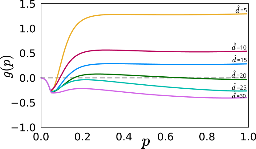
(a) $d=5$

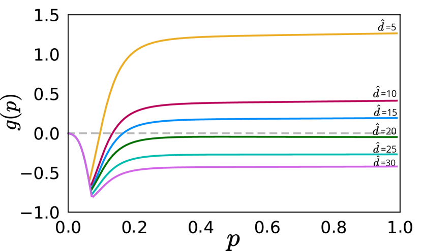
(b) $d=30$

Figure 2: Visualization of (11) over 40 nodes with (a) sparse contact graph; (b) dense contact graph. $A$ is fixed for all six curves shown, and different $\hat{A}$ with varying degree is generated randomly using [23]. Parameters: $\delta=1,\mu=0.1,\nu=3$.

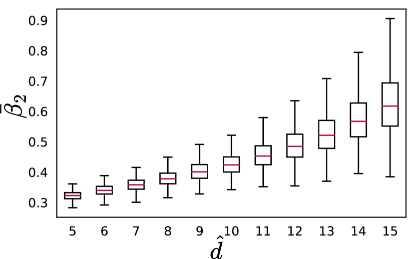
(a) $d=5$

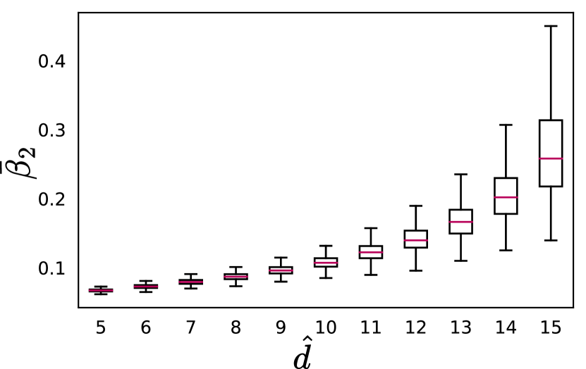
(b) $d=30$

Figure 3: Distribution of the critical point $\bar{\beta}_{2}$ of Theorem V.4 for 40 nodes with (a) sparse contact graph; (b) dense contact graph; and communication graphs of several representative degrees. Each box plot contains $\bar{\beta}_{2}$ from 1000 simulations. For each simulation, $A$ and $\hat{A}$ of appropriate $d$, $\hat{d}$ are generated randomly using [23]. Parameters: $\delta=1,\mu=0.1,\nu=3$.

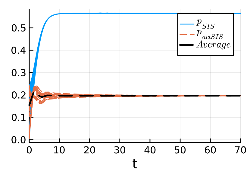
(a) $\bar{\beta}=0.23$.

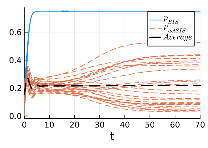
(b) $\bar{\beta}=0.4$.

Figure 4: Trajectories of network SIS and network actSIS dynamics over $26$-node regular graphs with $d=5$ and $\hat{d}=21$. Parameters: $\delta=0.5,\mu=0.2,\nu=8$ and $\tau_{s}=1$. Created using [21].

VI Numerical explorations

In Figure 5 we simulate the network actSIS model with a mixed-strategy network of $10$ agents: $5$ of them are risk-averters and $5$ are risk-ignorers (i.e. $\alpha_{j}(p_{s})=1$ for all $p_{s}$) as shown on the right. The simulation (left) shows that the infection level at the EE of the risk-averters is below the infection level of the risk-ignorers at the EE. This suggests that even when in contact with risk-ignorers, risk averters are able to maintain relatively low infection levels.

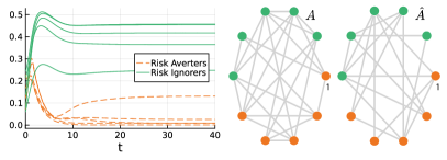
Figure 5: Simulations for a network of size $10$. Parameters: $\bar{\beta}=0.3,\delta=0.5,\tau_{s}=1,\mu=0.2$ and $\nu=8$. Nodes are numbered clockwise. Created using [21].

We also explore the result proved in Theorem V.3 for general contact networks. Figure 6 suggests that, even without the assumption of regularity for the contact matrices, the EE is reduced by the risk aversion strategy. We leave proving this general result to future work.

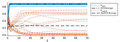
Figure 6: Simulations of (2) and (5),(6) over $26$ nodes. The matrices $A$ and $\hat{A}$ are symmetric and generated randomly. Contrary to the previous simulations, nodes are not required to have a fixed, or average, number of neighbors. Parameters: $\delta=0.5,\bar{\beta}=0.3,\tau_{s}=1,\mu=0.2,\nu=8$. Created using [21].

VII Discussion

We presented and analyzed network actSIS, a model of actively controlled SIS epidemics on networks of interconnected populations that adjust contact rates over a contact network in response to perceived infection risk based on observations over a communication network of population infection levels. We proved the onset of a transcritical bifurcation in the model. For regular contact and communication network graphs, we showed through proof and numerical simulation that the resulting endemic equilibrium is uniform and has a lower infection level than the endemic equilibrium of the uncontrolled network SIS model when populations use a risk aversion strategy. We further proved for regular graphs that this equilibrium can become unstable and undergo a bifurcation when the communication graph is sufficiently sparse. Simulations show that at this second bifurcation an endemic equilibrium with nonuniform levels of infection can emerge, despite the homogeneity in the system. In future work we will expand these analyses to general graphs that are not necessarily regular, and to strategies beyond risk aversion.

Appendix

Lyapunov-Schmidt Reduction for Theorem IV.2

At the singular point, we compute the leading order coefficients of the Lyapunov-Schmidt reduction, following [20, Chapter I, §3]: Define $\mathbf{x}=(\mathbf{p},\mathbf{p}_{s})$ and let $F(\mathbf{x},\bar{\beta})=\big{(}f(\mathbf{p},{\mathbf{p}}_{s},\bar{\beta}),g(\mathbf{p},{\mathbf{p}}_{s},\bar{\beta})\big{)}$ where $f,g$ are the right-hand side of (5),(6). Define the second order partial derivative of $F$ along vectors $\mathbf{y},\mathbf{z}$ and evaluated at some $(\mathbf{x}^{*},\bar{\beta}^{*})$ as

$$(d^{2}F)_{\mathbf{x}^{*},\bar{\beta}^{*}}(\mathbf{y},\mathbf{z})=\sum_{i=1}^{2N}\sum_{j=1}^{2N}\frac{\partial^{2}F}{\partial x_{i}\dots\partial x_{j}}(\mathbf{x}^{*},\bar{\beta}^{*})y_{i}z_{j}.$$ (14)

A first-order partial directional derivative is defined analogously. Note that at the bifurcation point $(\mathbf{x},\bar{\beta}^{*})$ the right and left eigenvectors of the Jacobian (8) are $\bar{\mathbf{v}}=(\mathbf{v^{*}},\hat{\Delta}^{-1}\hat{A}\mathbf{v}^{*})$ and $\bar{\mathbf{w}}=(\mathbf{w}^{*},\mathbf{0})$. The quadratic LS coefficient is

$$h_{xx}=\langle\bar{\mathbf{w}},d^{2}F_{0,\bar{\beta}^{*}}(\bar{\mathbf{v}},\bar{\mathbf{v}})\rangle\\ =\sum_{j=1}^{N}-w^{*}_{j}\bar{\beta}^{*}v^{*}_{j}\left(\sum_{m=1}^{N}\alpha_{j}(0)a_{jm}v^{*}_{m}+\sum_{l=1}^{N}\alpha_{j}(0)a_{jl}v^{*}_{l}\right)\\ +\sum_{j=1}^{N}w^{*}_{j}\sum_{l=1}^{N}\bar{\beta}^{*}a_{j}^{\prime}(0)a_{jl}v_{l}^{*}(\hat{\Delta}^{-1}\hat{A}\mathbf{v}^{*})_{j}\\ =\bar{\beta}^{*}\left(\sum_{i=1}^{N}w_{i}^{*}\left((\hat{\Delta}^{-1}\hat{A}\mathbf{v}^{*})_{i}(\alpha^{\prime}(0)A\mathbf{v}^{*})_{i}-2v_{i}^{*}(\alpha(0)A\mathbf{v}^{*})_{i}\right)\right).$$

Next, defining $\beta=\bar{\beta}-\bar{\beta}^{*}$ and $\tilde{A}=\operatorname{diag}\{(\alpha_{1}(0),\dots,\alpha_{N}(0)\}A$,

$$h_{x\beta}=\left\langle\bar{\mathbf{w}},d\left(\frac{\partial F}{\partial\beta}\right)_{0,\bar{\beta}^{*}}(\bar{\mathbf{v}})\right\rangle=\langle\mathbf{w}^{*},\tilde{A}\mathbf{v}^{*}\rangle=\sum_{i=1}^{N}w_{i}(\tilde{A}\mathbf{v}_{i})^{*}$$

and note that $h_{x\beta}>0$.

References

- [1] W. Mei, S. Mohagheghi, S. Zampieri, and F. Bullo, “On the dynamics of deterministic epidemic propagation over networks,” Annual Reviews in Control, vol. 44, pp. 116–128, 2017.
- [2] L. Zino and M. Cao, “Analysis, prediction, and control of epidemics: A survey from scalar to dynamic network models,” IEEE Circuits and Systems Magazine, vol. 21, no. 4, pp. 4–23, 2021.
- [3] L. Yang, S. M. Constantino, B. T. Grenfell, E. U. Weber, S. A. Levin, and V. V. Vasconcelos, “Sociocultural determinants of global mask-wearing behavior,” Proceedings of the National Academy of Sciences, vol. 119, no. 41, p. e2213525119, 2022.
- [4] M. Ye, L. Zino, A. Rizzo, and M. Cao, “Game-theoretic modeling of collective decision making during epidemics,” Physical Review E, vol. 104, no. 2, p. 024314, 2021.
- [5] K. Frieswijk, L. Zino, M. Ye, A. Rizzo, and M. Cao, “A mean-field analysis of a network behavioral–epidemic model,” IEEE Control Systems Letters, vol. 6, pp. 2533–2538, 2022.
- [6] U. Maitra, A. R. Hota, and V. Srivastava, “SIS epidemic propagation under strategic non-myopic protection: A dynamic population game approach,” IEEE Control Systems Letters, 2023.
- [7] A. Satapathi, N. K. Dhar, A. R. Hota, and V. Srivastava, “Coupled evolutionary behavioral and disease dynamics under reinfection risk,” IEEE Transactions on Control of Network Systems, 2023.
- [8] W. Xuan, R. Ren, P. E. Paré, M. Ye, S. Ruf, and J. Liu, “On a network SIS model with opinion dynamics,” IFAC-PapersOnLine, vol. 53, no. 2, pp. 2582–2587, 2020.
- [9] B. She, J. Liu, S. Sundaram, and P. E. Paré, “On a networked sis epidemic model with cooperative and antagonistic opinion dynamics,” IEEE Transactions on Control of Network Systems, vol. 9, no. 3, pp. 1154–1165, 2022.
- [10] P. E. Paré, A. Janson, S. Gracy, J. Liu, H. Sandberg, and K. H. Johansson, “Multilayer SIS model with an infrastructure network,” IEEE Transactions on Control of Network Systems, vol. 10, no. 1, pp. 295–307, 2022.
- [11] V. Abhishek and V. Srivastava, “SIS epidemic spreading under multi-layer population dispersal in patchy environments,” IEEE Transactions on Control of Network Systems, 2023.
- [12] Y. Wang, S. Gracy, H. Ishii, and K. H. Johansson, “Suppressing the endemic equilibrium in SIS epidemics: A state dependent approach,” IFAC-PapersOnLine, vol. 54, no. 15, pp. 163–168, 2021.
- [13] Y. Wang, S. Gracy, C. A. Uribe, H. Ishii, and K. H. Johansson, “A state feedback controller for mitigation of continuous-time networked SIS epidemics,” IFAC-PapersOnLine, vol. 55, no. 41, pp. 89–94, 2022.
- [14] L. Walsh, M. Ye, B. Anderson, and Z. Sun, “Decentralised adaptive-gain control for eliminating epidemic spreading on networks,” arXiv preprint arXiv:2305.16658, 2023.
- [15] Y. Zhou, S. A. Levin, and N. E. Leonard, “Active control and sustained oscillations in actSIS epidemic dynamics,” IFAC-PapersOnLine, vol. 53, no. 5, pp. 807–812, 2020.
- [16] R. Pagliara and N. E. Leonard, “Adaptive susceptibility and heterogeneity in contagion models on networks,” IEEE Transactions on Automatic Control, vol. 66, no. 2, pp. 581–594, 2020.
- [17] F. Blanchini and S. Miani, Set-theoretic methods in control, vol. 78. Springer, 2008.
- [18] H. K. Khalil, Nonlinear Systems. Upper Saddle River, NJ: Prentice Hall, 3 ed., 2002.
- [19] J. Guckenheimer and P. Holmes, Nonlinear Oscillations, Dynamical Systems, and Bifurcations of Vector Fields, vol. 42. New York, NY: Springer-Verlag, 2013.
- [20] M. Golubitsky and D. G. Schaeffer, Singularities and Groups in Bifurcation Theory, vol. 51 of Applied Mathematical Sciences. New York, NY: Springer-Verlag, 1985.
- [21] C. Rackauckas and Q. Nie, “DifferentialEquations.jl–a performant and feature-rich ecosystem for solving differential equations in Julia,” Journal of Open Research Software, vol. 5, no. 1, 2017.
- [22] D. V. Ouellette, “Schur complements and statistics,” Linear Algebra and its Applications, vol. 36, pp. 187–295, 1981.
- [23] A. Hagberg, P. Swart, and D. S Chult, “Exploring network structure, dynamics, and function using networkx,” tech. rep., Los Alamos National Lab.(LANL), Los Alamos, NM (United States), 2008.