Localization and integrability breaking in weakly interacting Floquet circuits

Abstract

We present a family of Floquet circuits that can interpolate between non-interacting qubits, free propagation, generic interacting, and dual-unitary dynamics. We identify the operator entanglement entropy of the two-qubit gate as a good quantitative measure of the interaction strength. We test the persistence of localization in the vicinity of the non-interacting point by probing spectral statistics, decay of autocorrelators, and measuring entanglement growth. The finite-size analysis suggests that the many-body localized regime does not persist in the thermodynamic limit. Instead, our results are compatible with an integrability-breaking phenomenon.

I Introduction

Thermalization of quantum many-body systems has been an active topic of research in recent years Nandkishore and Huse (2015); Abanin et al. (2019); Ueda (2020). It is now known that generic interacting systems reach an equilibrium state that can be described by a statistical mechanics ensemble Deutsch (1991); Srednicki (1994); Rigol et al. (2008). Such systems show quantum chaotic dynamics, which encompasses several dynamical and static traits Heller (2001); D’Alessio et al. (2016). There are two non-generic cases where the dynamics is not expected to be chaotic: (i) non-interacting systems can show free propagation or get localized in the presence of disorder, the latest being called Anderson localization Anderson (1958). (ii) Interacting integrable systems whose extensive number of conserved quantities constrained their dynamics, giving rise to a special type of thermalization Vidmar and Rigol (2016). When integrability is perturbed in an extensive manner, quantum chaos is expected to set in the long run and the system thermalizes Brenes et al. (2020); Rigol (2016); Essler and Fagotti (2016); D’Alessio et al. (2016); Rigol et al. (2007). However, in recent years, it was shown that strong disorder potentials may cause the break down of thermalization, the so-called many-body localization (MBL) Basko et al. (2006); Gornyi et al. (2005); Oganesyan and Huse (2007). This is described as an ergodicity-breaking transition at finite interaction strength and disorder. In this regime, quasi-local conserved quantities Huse et al. (2014); Serbyn et al. (2013) are stabilized, leading to emergent integrability out of an initially quantum chaotic system. There are lots of evidence of MBL in systems of moderate size Schreiber et al. (2015); Luitz et al. (2015), but recently, the fate of MBL in the thermodynamic limit has been put into question Šuntajs et al. (2020); Sels and Polkovnikov (2023, 2021); Kiefer-Emmanouilidis et al. (2021) and spark debates on the scaling of the critical disorder and possible de-localization mechanisms Morningstar et al. (2022); Sels (2022); Crowley and Chandran (2020); Sierant and Zakrzewski (2022); Sierant et al. (2020); Panda et al. (2020); Crowley and Chandran (2022).

An interesting question arises at the intersection of the dynamical regimes exposed above: how stable are Anderson localized systems to small interactions? On the one hand, any small interactions are expected to drive the system towards thermal equilibrium, on the other hand, disorder may overcome the interactions and the system becomes MBL. In Ref. Laflorencie et al. (2022) the authors studied a model where the MBL persists at small enough interactions. The critical value of the localization length is the one expected from the avalanche mechanism De Roeck and Imbrie (2017); Thiery et al. (2018). In Ref. Krajewski et al. (2022) it is shown that small interactions are not effectively perturbing the Anderson localized orbitals when the disorder strength is large. In this work, we study the onset of chaos in a maximally localized system subjected to small and medium-strength interactions.

Most of the studies that address the strong disorder and weak interaction limit focus on Hamiltonian systems so far. Here we present a family of Floquet circuits that can interpolate between non-interacting qubits and strongly interacting systems. In this work, we test the onset of quantum chaos close to the trivial non-interacting point and study the fate of the MBL regime with increasing system size in our model. Our results suggest that there exists no MBL phase for our system in the thermodynamic limit. Instead, our numerics suggest a finite-size crossover similar to integrability-breaking phenomena Bulchandani et al. (2022).

The structure of the paper is as follows: In Sec. II, we introduce our Floquet model and the quantities we use to study the onset of quantum chaos. In Sec. III, we present our results for various commonly studied quantities in the field of thermalization, together with a finite-size scaling analysis. Finally in Sec. IV we discuss the implications and perspectives of our work.

II Model and observables

Before we present our results, we provide technical details about our model and different quantities to detect signatures of the MBL-regime.

II.1 Classification of two-qubit gates

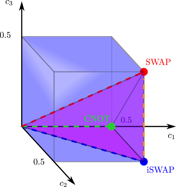
Figure 1: Parametrization of different equivalence classes for two-qubit gates: Each two-qubit gate is uniquely determined up to single-qubit unitaries by three parameters ${0\leq c_{3}\leq c_{2}\leq c_{1}\leq 0.5}$ (purple tetrahedron) that form the Weyl chamber. Colored points indicate common gates. the dashed lines show the corresponding families of two-qubit gates defined in Sec. II.3.

For any two-qubit gate $U_{2}$, there exist general single-qubit gates $u_{1},\,u_{2},v_{1}$ and $v_{2}$ and a two-qubit gate of the form (with $\bm{c}=(c_{1},c_{2},c_{3})$)

$$G(\bm{c})=\exp\left[-i\dfrac{\pi}{2}\left(c_{1}\sigma^{x}\otimes\sigma^{x}+c_{2}\sigma^{y}\otimes\sigma^{y}+c_{3}\sigma^{z}\otimes\sigma^{z}\right)\right],$$ (1)

such that it can be decomposed as  Kraus and Cirac (2001)

$$U_{2}=(u_{1}\otimes u_{2})G(v_{1}\otimes v_{2}),$$ (2)

Here $\sigma^{\alpha}$ with $\alpha=x,y,z$ are the Pauli operators acting on each qubit.

Restricting to the subset ${0.5\geq c_{1}\geq c_{2}\geq c_{3}\geq 0}$, this allows for a classification of all two-qubit gates in terms of the vector $\bm{c}$: Two gates which are described by the same vector $\bm{c}$ are equivalent to each other apart from the multiplication with single-qubit gates Balakrishnan and Sankaranarayanan (2011a, 2010).

The space enclosed by the independent set of $\mathbf{c}$ is known as the Weyl chamber Balakrishnan and Sankaranarayanan (2009); Zhang et al. (2003); Makhlin (2002) and indicated by the purple tetrahedron in Fig. 1. There are a few special points and lines Balakrishnan and Sankaranarayanan (2011a)(see Fig. 1):

1. $c_{1}=c_{2}=c_{3}=0$ corresponds to independent single-qubit rotations.

2. $c_{1}=c_{2}=c_{3}=0.5$ is the equivalence class of the SWAP gate up to single qubit rotations.

3. $c_{1}=c_{2}=0.5$ and $c_{3}\geq 0$ denote the family of dual-unitary gates (shown as an orange line in Fig. 1).

4. $c_{1}=0.5$ and $c_{2}=c_{3}=0$ is the CNOT gate up to single qubit rotations.

Since any two-qubit gate corresponds to a specific point of the Weyl chamber, the entanglement properties of each gate Eq. (2) are uniquely determined by the vector ${\bm{c}=(c_{1},c_{2},c_{3})}$ Balakrishnan and Sankaranarayanan (2010, 2011b, 2011a).

II.2 Two-qubit gate entanglement

One way to characterize equivalence classes of two-qubit gates defined in Eq. (2) is by their operator Schmidt decomposition Balakrishnan and Sankaranarayanan (2011b):

$$U_{2}=\sum_{l=1}^{4}\lambda_{l}(A_{l}\otimes B_{l}),$$ (3)

where $A_{l}$ and $B_{l}$ are orthonormal operators for the corresponding single-qubit spaces. This is analogous to the Schmidt decomposition of states. The Schmidt coefficients $\lambda_{l}$ are normalized, i.e. $\sum_{l=1}^{4}\lambda_{l}=1$. It turns out that two-qubit gates Eq. (2) that are different only in single-qubit rotations will have the same set of Schmidt coefficients Balakrishnan and Sankaranarayanan (2011b). Henceforth, the set $(c_{1},c_{2},c_{3})$ uniquely determines any function of the Schmidt coefficients. In the following, We use the second Renyi entropy Balakrishnan and Sankaranarayanan (2011b, a) which allows us to define the operator entanglement per gate as:

$$s(\bm{c})=-\log\left(\sum_{l=1}^{4}\lambda^{2}_{l}\right).$$ (4)

There are a few remarks with respect to the operator entanglement for some regions in the Weyl chamber. First, the line $c_{1}=c_{2}=0.5$, $c_{3}<0.5$ has the largest possible $s(\bm{c})=2\log 2$ Balakrishnan and Sankaranarayanan (2011b). They are the building block of so-called dual-unitary circuits Bertini et al. (2019a); Bertini and Piroli (2020); Akila et al. (2016), which exhibit the fastest scrambling in the family of random circuits Bensa and Žnidarič (2021); Zhou and Harrow (2022). Recently, it was shown that after perturbing the dual unitary point the gate operator entanglement plays a crucial role in recovering the more generic quantum chaotic behavior Rampp et al. (2023). This motivates our choice to study long-time many-body properties - i.e., scrambling, chaos and localization - of quantum circuits as a function of the operator entanglement of the two-qubit gate they consist of.

The operator entanglement at any point of the Weyl chamber is given by Balakrishnan and Sankaranarayanan (2011b):

$$s(\bm{c})=-\log(P(\bm{c})/32),$$ (5)

with

$$P(\bm{c})=14+4\cos(2\pi c_{1})+4\cos(2\pi c_{2})+4\cos(2\pi c_{3})+$$

$$\cos(2\pi(c_{1}-c_{2}))+\cos(2\pi(c_{1}+c_{2}))+\cos(2\pi(c_{1}-c_{3}))+$$

$$\cos(2\pi(c_{1}+c_{3}))+\cos(2\pi(c_{2}+c_{3}))+\cos(2\pi(c_{2}-c_{3})).$$ (6)

II.3 Floquet circuit model

$$U=\leavevmode\hbox to116.48pt{\vbox to77.62pt{\text{[drawing]}}}\hskip 8.5359pt{\left\uparrow\vbox to39.83368pt{}\right.\kern-1.2pt}t u_{1} u_{2} u_{3} u_{4} u_{5} u_{6} u_{7} u_{8} w_{1} w_{2} w_{3} w_{4} w_{5} w_{6} w_{7} w_{8} G(\bm{c}) G(\bm{c}) G(\bm{c}) G(\bm{c}) G(\bm{c}) G(\bm{c}) G(\bm{c})$$

Figure 2: Diagrammatic notation of the unitary defined in Eq. (7). The single-qubit gates $u_{i}$ and $w_{i}$ introduce spatial disorder to the system, while the interaction between neighboring qubit is mediated by the two-qubit gate $G(\mathbf{c})$.

The characterization of two-qubit unitaries by means of the gate $G(\mathbf{c})$ allows us to introduce the following family of Floquet circuits:

$$U(\bm{c})=\prod_{i=0}^{L-1}w_{i}\prod_{k=0}^{L/2-2}G(\bm{c})_{2k+1,2k+2}\prod_{i=0}^{L-1}u_{i}\prod_{k=0}^{L/2-1}G(\bm{c})_{2k,2k+1}$$ (7)

A diagrammatic representation of this circuit is shown in Fig. 2: The gates $u_{i}$ and $w_{i}$ are single qubit rotations drawn from the Haar measure. They act as a spatial disorder. The gate $G(\bm{c})$ is defined in equation Eq. (1). All bonds have the same set of parameters ${\bm{c}=(c_{1},c_{2},c_{3})}$. The Floquet dynamics is given by repeatedly applying $U$ Eq. (7), thus the Floquet circuit ensemble is determined by the vector $\bm{c}$.

A few special cases of this model have been already studied in the literature: The case of space-time dual unitary circuits $c_{1}=c_{2}=0.5$, $c_{3}\geq 0$ (see orange dashed line in Fig. 1) has been extensively studied Bertini et al. (2019b); Fisher et al. (2023). These circuits are quantum chaotic despite being exactly solvable, which makes them special in the study of thermalization Piroli et al. (2020); Bertini et al. (2020a, b); Claeys and Lamacraft (2021); Aravinda et al. (2021); Bertini et al. (2021, 2018); Borsi and Pozsgay (2022). For instance, they are shown to saturate bounds on information scrambling Aravinda et al. (2021); Bertini et al. (2019c); Bertini and Piroli (2020); Zhou and Harrow (2022). A random version of this circuit - different single qubit gates at each time step - was studied in Ref. Bensa and Žnidarič (2021), the authors found that the fastest scrambler quantum circuit, i.e., highest entanglement rate production, are random circuits with $c_{1}=c_{2}=0.5$ and $c_{3}\geq 0$.

The vicinity of the non-interacting point $c_{1}=c_{2}=c_{3}=0$ is less explored. A natural question is whether the system gets many-body localized Abanin et al. (2019); Alet and Laflorencie (2018) for small finite values of the coefficients $(c_{1},c_{2},c_{3})$. In principle, there are multiple possible choices for $\bm{c}$ that can be studied starting from the origin. We focus on three lines:

1. SWAP line: it is determined by $c_{1}=c_{2}=c_{3}$ with $0<c_{1}<0.5$ (see Fig 1). It interpolates between single qubit rotations ($c_{1}=0$) and the SWAP gate ($c_{1}=0.5$).

2. CNOT line: denoted by $c_{2}=c_{3}=0$ and $0<c_{1}<0.5$, this line ends on a CNOT gate-based circuit.

3. The imaginary SWAP (iSWAP) Foxen et al. (2020) line given by $c_{3}=0$, $c_{1}=c_{2}$ and $0<c_{1}<0.5$ that ends on the imaginary-SWAP gate $c_{1}=c_{2}=0.5$.

In Ref. Garratt and Chalker (2021) the authors report MBL for small coefficients on the SWAP line. Besides the three lines mentioned above, we study a subset $\mathbf{c}=(c_{1},c_{2},c_{3})$ with $c_{1},c_{2}\in(0.02,0.28)$ and $c_{3}\in(0.0,0.18)$ in order to test the generality of the chosen lines and possible links between long-time dynamics and two-qubit gate invariants.

II.4 Level statistics and eigenstate entanglement entropy

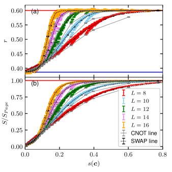
Figure 3: Gap ratio (upper panel) and eigenstate entanglement entropy (lower panel) for system sizes $L=8,10,12,14,16$ and combination of values: $c_{1},c_{2}=0.02,0.04,0.06,...,0.2,0.24,0.28$ and $c_{3}=0,0.02,0.04,...,0.18$. SWAP line (black dashed) and CNOT line (grey continuous) are also shown for comparison. Error bars are $68\%$ confidence interval.

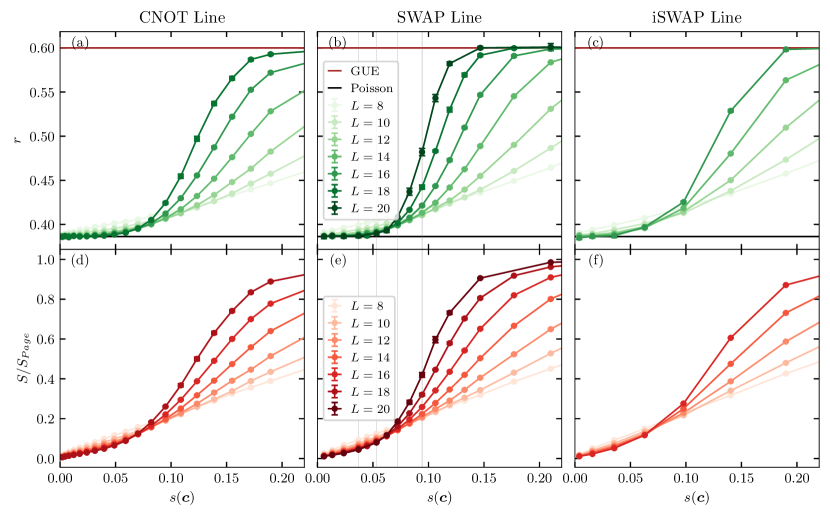
Figure 4: Upper row (a,b,c): Gap ratio as function of the two-qubit-gate operator entanglement entropy for system sizes $L=8,10,12,14,16$ (in addition CNOT line has $L=18$ and SWAP line has $L=18,20$). Lower row (d,e,f): Average entanglement entropy normalized by the Page value $S_{\text{Page}}=0.5(L\log 2-1)$ for the same system sizes. Right column: CNOT line denoted by $c_{1}\in[0.02,0.40]$, $c_{2}=c_{3}=0$. Middle column: SWAP line denoted as $c_{1}=c_{2}=c_{3}$ with $c_{1}\in[0.02,0.40]$. Left column: DU line denoted by $c_{2}=c_{1}$, $c_{3}=0$ and $c_{1}\in[0.02,0.28]$. Error bars (too small for this scale) are $68\%$ confidence interval. Grey vertical lines are the $s(\bm{c})$ for which dynamics is shown in Sec. III.2. In all three cases, the operator entanglement entropy $s(\bm{c})$ indicates an MBL-to-thermal crossover for both gap ratio and eigenstate entanglement entropy.

The long-time dynamics of Floquet circuits can be probed by the spectral properties of the Floquet operator D’Alessio et al. (2016). In particular, we are interested in the eigenphases and eigenstates $U|n\rangle=e^{i\theta_{n}}|n\rangle$. The gaps between consecutive eigenphases are defined as $\delta_{i}=\theta_{i+1}-\theta_{i}$, the ratio between two consecutive gaps is denoted as:

$$r_{i}=\min\left(\delta_{i+1},\delta_{i}\right)/\max\left(\delta_{i+1},\delta_{i}\right).$$ (8)

The average gap ratio $r$ is known to serve as an order parameter for ergodicity breaking transitions Pal and Huse (2010); Luitz et al. (2015): When the Floquet dynamics leads to thermalization, the mean gap ratio is described by GUE random matrix ensemble $\overline{r}\approx 0.60$ Atas et al. (2013). In contrast, when the Floquet dynamics gets localized, i.e. MBL, the gap ratio statistics is Poissonian such that $\overline{r}=2\log 2-1\approx 0.386$ Oganesyan and Huse (2007); D’Alessio et al. (2016). If our Floquet model undergoes a MBL transition it should show up in the behavior of $r$ as a function of the Schmidt coefficients.

A second diagnostic for the transition is the structure of eigenstates of the time evolution operator: We introduce the reduced density matrix over half of the spin chain as $\rho_{A}=\operatorname{Tr}_{L/2}\left(|n\rangle\langle n|\right)$. We probe the transition at the level of eigenstates using the half-chain entanglement entropy

$$S=-\operatorname{Tr}\rho_{A}\log\rho_{A}.$$ (9)

In the thermal phase, the eigenstates are expected to be essentially random vectors in Hilbert space; thus their entanglement entropy is proportional to the chain length $S_{\text{Page}}=(L\log 2-1)/2$, the so-called Page value Page (1993). On the other hand, in the localized phase the eigenstates only exhibit short-range entanglement, resulting in an area law for the entanglement entropy $S\approx const$ Nandkishore and Huse (2015). Hence the average entanglement entropy $\overline{S}$ signals the MBL transition Khemani et al. (2017); Luitz et al. (2015); Yu et al. (2016).

These quantities are obtained using exact diagonalization. For small system sizes $L=8,10,12$ the whole eigenspectrum can be computed, while for larger system sizes $L\geq 14$ polynomial filtered diagonalization Luitz (2021) is used for extracting 100 eigenpairs of the Floquet unitary. All quantities are averaged over 3000-6000 disorder realizations (except for $L=20$ where only 500-1000 realizations are used) and all available eigenstates.

II.5 Quench dynamics

Another direct way to detect localization in our system is using transport properties. A common tool is the autocorrelator Long et al. (2023); Schreiber et al. (2015); Luitz et al. (2016); Lezama et al. (2019, 2021):

$$C(t)=\dfrac{1}{2^{L}}\operatorname{Tr}\left[\hat{O}(t)\hat{O}\right]=\dfrac{1}{2^{L}}\operatorname{Tr}\left[(\hat{U}^{\dagger}(t)\hat{O}\hat{U}(t)\hat{O}\right].$$ (10)

Here $O$ is a normalized observable with vanishing mean ($\operatorname{Tr}{\hat{O}}=0$, $\operatorname{Tr}{\hat{O}^{2}}=2^{L}$), and the time evolution is generated by the circuit introduced in Eq. (7), i.e. $\hat{U}(t)=U(\bm{c})^{t}$.

Since our goal is to probe scrambling caused by the entangling gates, we choose an operator $\hat{O}$ such that $C(t)=1$ for $c_{1}=c_{2}=c_{3}=0$. To achieve this, consider the product of the single-site operators at $i=\lfloor L/2\rfloor$:

$$R=u_{i}w_{i}$$ (11)

Since $R$ is unitary, there exists a diagonal matrix $D$ and an unitary $V$ such that

$$R=V^{\dagger}DV.$$ (12)

By choosing

$$\hat{O}=V^{\dagger}\sigma^{z}_{i}V$$ (13)

we obtain an autocorrelator $C(t)$ with the desired properties. It is important to note that the choice of $V$ depends on the specific disorder configuration. When the system thermalizes, the disorder-averaged autocorrelator vanishes in the long-time limit Nandkishore and Huse (2015). In contrast, $C(t)$ is expected to converge to a non-zero value in the MBL regime Nandkishore and Huse (2015). In summary, we obtain

$$\lim_{t\rightarrow\infty}C(t)=\begin{cases}0,&\text{thermalization}\\ c>0,&\text{localization}.\\ \end{cases}$$ (14)

Another way to probe transport properties in the study of MBL is the entanglement entropy production starting from a product state $|\psi(0)\rangle=|\psi_{0}\rangle$ Žnidarič et al. (2008); Kjäll et al. (2014). Analog to Sec. II.4, we compute the half-chain entanglement entropy $S(t)$ [cf. Eq.(9)], but now for the time-evolved state $|\psi(t)\rangle$ instead. The entanglement growth rate depends on the overall dynamics: quantum chaotic systems show linear growth in time, while MBL systems exhibit logarithmic growth of entanglement Žnidarič et al. (2008); Bardarson et al. (2012). The latest signals the existence of quasi-local integrals of motion Serbyn et al. (2013); Huse et al. (2014).

III Results

III.1 Gap ratio and eigenstate entanglement entropy

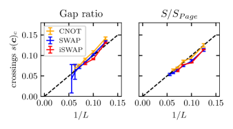
Figure 5: Crossings of the curves in Fig. 4 between system size $L$ and $L+2$ for the gap ratio (a) and eigenstate entanglement entropy (b) along the CNOT line (orange), SWAP line (blue), iSWAP line (red). The black dashed lines show the scaling $1/L$. For accessible system sizes the trend is compatible within error bars with $s(\bm{c})_{c}\propto 1/L$, suggesting restoring of ergodicity in the thermodynamic limit for any finite interaction strength.

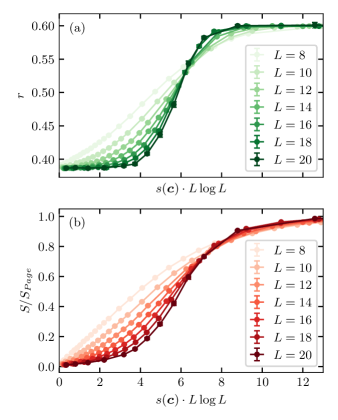
Figure 6: (a) Gap ratio and (b) entanglement entropy along the SWAP line for system size $L=8-20$. The two-qubit gate operator entanglement $s(\bm{c})$ is re-scaled by $L\log L$. The data set is the same as shown in Fig. 4. These visible crossings suggest a drifting critical value $s(\bm{c})_{crit}\propto 1/L$, compatible with an integrability-breaking phenomenon (see main text).

As a first check, we probe the operator entanglement per gate $s(\bm{c})$ as a unifying parameter for the interaction strength. To do so, we show the gap ratio and the eigenstate entanglement entropy as a function of the gate entanglement entropy $s(\bm{c})$ in Fig. 3 (a) and (b), respectively. We focus on parameters $\bm{c}(c_{1},c_{2},c_{3})$ within the range $c_{1},c_{2}=[0.02,0.28]$ and $c_{3}=[0.0,0.18]$. For the system size and $s(\bm{c})$ fixed, the gap ratio and half-chain entanglement almost collapse on top of the corresponding SWAP line value. This supports our motivation to choose $s(\bm{c})$ as an indicator for the interaction strength.

However, the results for the CNOT and the SWAP line lie not directly on top of each other. This difference may originate from the specific choice of the vector $\bm{c}$. On the CNOT line, two Schmidt coefficients $\lambda_{l}$ [cf. Eq. (8)] are zero Balakrishnan and Sankaranarayanan (2011b), which is not the case for any other choice of $\bm{c}$ in the Weyl chamber. Therefore the finite size behavior visible in $r$ and $S/S_{\text{Page}}$ may be affected by this choice of $\bm{c}$ (see Appendix A for a more quantitative comparison).

For our further studies, we choose three parameter lines that differ in the number of non-vanishing coefficients $c_{i}$: the SWAP line, the iSWAP line, and the CNOT line (cf Sec. II.3). The gap ratio and the half-chain entanglement entropy on these lines of the Weyl chamber and systems sizes are shown in Fig. 4. In all three cases, we see a crossover between an MBL regime (indicated by a small eigenstate entanglement entropy and an $r$-value close to the Poissonian case) for small interactions towards a thermal regime at large interactions. Besides, an analysis of the entanglement entropy fluctuations is shown in Appendix Sec. B.

Furthermore, the curves of different system sizes intersect. We then compare the different crossings between consecutive system sizes in order to check the stability of the phase in the thermodynamic limit Pal and Huse (2010). In Fig. 5, the crossings of gap ratio and entanglement entropy for consecutive sizes $L$ and $L+2$ are shown. The trend of the crossing suggests a scaling $\propto 1/L$, at least for the accessible system sizes. Remarkably, finite size effects for the half-chain entanglement entropy are less pronounced in comparison to the r-value. The trend of the data suggests that the crossings are shifting towards zero in the limit $L\rightarrow\infty$, thus ergodicity is restored at any finite interaction. However, given the smallness of the accessible system sizes, we can not rule out a change in the trend at larger sizes.

It has been recently shown that non-interacting spin systems with small perturbative interaction undergo a Fock space type delocalization “transition” that marks the onset of quantum chaos Bulchandani et al. (2022). Taking $\epsilon$ as the integrability breaking parameter, the value $\epsilon_{c}$ denotes the onset of chaos scaling as $\epsilon_{c}\sim(L\log L)^{-1}$ with increasing system size. In Fig. 6 we test such scaling for $s(\bm{c})$ for both gap ratio and eigenstate entanglement entropy. Although the available system sizes do not allow us to discern the $\log L$ component, the linear scaling is clearly visible. From this perspective, the MBL-thermalization crossover appears as an ordinary integrability-breaking phenomenon for finite system sizes.

III.2 Single spin autocorrelation and entanglement entropy after a quench

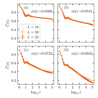
Figure 7: Single spin autocorrelation $\overline{C}(t)$ as a function of time $t$, gates $G(\bm{c})$ are chosen on the SWAP line for $c=(0.05,0.06,0.07,0.08)$ (the corresponding interaction strength $s(\bm{c})$ is shown in each panel). Disorder average is taken over 1000-4000 disorder realizations. Errors bars are $68\%$ confidence interval.

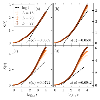
Figure 8: Half chain entanglement entropy after a quench on the SWAP line for $c=(0.05,0.06,0.07,0.08)$ (same values but translated to $opEE$ are shown in each panel) and system sizes $L=18,20,22$. Disorder average is taken over 1000-4000 disorder realizations, error bars denote $68\%$ confidence interval. The black dashed lines are $\log t$ with different offsets. For large interactions $S(t)$ the logarithmic growth is proceeded by a faster entanglement entropy growth.

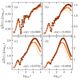
Figure 9: Numerical derivative of the half chain entanglement entropy with respect to $\log t$ after a quench on the SWAP line for $c=(0.05,0.06,0.07,0.08)$ (same data is shown in Fig. 8) and system sizes $L=18,20,22$. The entropy growth is faster than pure logarithmic for all interaction strengths.

From the previous section, we can conclude that the critical operator entanglement per gate $s(\bm{c})$ is scaling roughly as $1/L$. The largest system size for which we could extract eigenvalues and eigenvectors is $L=20$. From Fig. 5, we estimate the crossover region for current system sizes to be around $s(\bm{c})\sim 1/20=0.05$. In this section, we explore signatures for this crossover in quench dynamics for up to $10^{5}$ cycles in the regime $s(\bm{c})\lesssim 0.1$ and system sizes $L\geq 18$.

In Fig. 7, we show the autocorrelation function introduced in Sec. II.5 on the SWAP line of the model. The circuit dynamics is simulated using Cirq Developers (2023) that allows to reach $10^{5}$ cycles and up to $L=22$ qubits.

For $s(\bm{c})\approx 0.09,0.07$ close to the crossover region, $\overline{C}(t)$ decays with a scale either logarithmically or stretched exponentially, in line with previous work on autocorrelation decay in prethermal systems Long et al. (2023). The long-time limit $\lim_{t\rightarrow\infty}C(t)$ decreases with system size, suggesting a trend towards thermalization. For smaller interactions $s(\bm{c})\approx 0.05,0.03$, our accessible time-scales are too short to draw conclusions about a drift in the long-time dynamics: we do not reach a steady state in our numerics.

Finally, we study the entanglement entropy growth for initial product states along the SWAP line. As discussed in Sec. II.5, a signature of localization is logarithmic entanglement growth. As is visible in Fig. 8, the entanglement entropy $S(t)$ is growing faster than logarithmically (black dashed lines) at time scales $t\gtrsim 10^{3}$ and interactions $s(\bm{c})\gtrsim 0.07$. In order to confirm this observation, we compute the derivative of $S(t)$ with respect to $\log t$ (see Fig. 9). A logarithmic curve would be visible as a constant value. Instead, we see that the derivative keeps growing with system size even in the regime when the level statistics is Poissonian $s(c)=0.0369$. We conclude that the entropy growth is faster than pure logarithmic growth even for the smallest interactions. The latest is in odds with the steady logarithmic growth in MBL regimes Bardarson et al. (2012).

IV Discussion

In this work, we have introduced a generic Floquet circuit model that allows us to parametrically tune the interaction and keep the disorder maximal. We have identified the gate entanglement entropy $s(\bm{c})$ as a quantitative measure for the interaction. In the limit $s(\bm{c})=0$, our model reduces to a non-interacting system. Our results for various quantities suggest that the observed MBL regime for small interactions does not persist in the thermodynamic limit. Moreover, by re-scaling our results with the gate entanglement $s(\bm{c})$, we conclude that this crossover at finite system sizes shows a striking similarity to an integrability-breaking transition Bulchandani et al. (2022).

Our reachable system sizes and our investigated model are not sufficient to draw conclusions about the general fate of the MBL transition in the thermodynamic limit. Nevertheless, they suggest analyzing whether the results for other commonly studied models in the field of many-body localization are in alignment with an integrability-breaking transition Krajewski et al. (2022, 2023). Apart from that, our model contains dual unitary circuits as another special case for a specific choice of parameters $\bm{c}$. This model is thus a good starting point to study the effects of breaking dual-unitarity in more detail Rampp et al. (2023).

V Acknowledgments

We thank Anushya Chandran, Pieter Claeys, David Long, David Luitz and Michael Rampp for inspiring discussions. L.C. gratefully acknowledges funding by the U.S. ARO Grant No. W911NF-21-1-0007. All statements of fact, opinion or conclusions contained herein are those of the authors and should not be construed as representing the official views or policies of the US Government.

Appendix A Gate operator entanglement, SWAP and CNOT lines

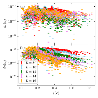
Figure 10: Distance of (a) the gap ratio $r(\bm{c},L)$ and (b) entanglement entropy $S(\bm{c},L)$ to the reference values $r(\bm{c}_{S},L)$ and $S(\bm{c}_{S},L)$ on the SWAP line. Dashed lines are error bars of $r(\bm{c}_{S},L)$ and $S(\bm{c}_{S},L)$. The SWAP reference points are computed by using spline interpolation of the curves shown in Fig. 4. The points are the same data as shown in Fig. 3.

Throughout this work, we assume that the results for the SWAP, iSWAP and CNOT line can be extrapolated to any other set of $\bm{c}=(c_{1},c_{2},c_{3})$ via the equivalence through the gate operator entanglement $s(\bm{c})$. Inspired by Ref. Rampp et al. (2023), where the authors found that $s(\bm{c})$ plays a leading role in generic thermalization, we aim to apply these ideas to the weakly interacting regime. In this section, we provide quantitative tests for this assumption by computing the gap ratio and eigenstate operator entanglement at any point $(c_{1},c_{2},c_{3})$, namely $r(\bm{c},L)$ and $S(\bm{c},L)$, and the difference

$$d_{r}(\bm{c}) =|r(\bm{c},L)-r(\bm{c}_{S},L)|$$ (15)

$$d_{S}(\bm{c}) =|S(\bm{c},L)-S(\bm{c}_{S},L)|/S_{Page},$$ (16)

where $r(\bm{c}_{S},L)$ and $S(\bm{c}_{S},L)$ are the gap ratio and eigenstate entanglement entropy for the reference choice ${\bm{c}_{S}=(c_{x},c_{x},c_{x})}$ on the SWAP line and the same gate operator entanglement entropy $s(\bm{c})=s(\bm{c}_{S})$. Our results are shown in Fig. 10. As a reference, we compare these results with the effects of the statistical error of $r(\bm{c}_{S},L)$ and $S(\bm{c}_{S},L)$ due to the disorder average, indicated by dashed lines. When a point $d_{r}(\bm{c})$ or $d_{S}(\bm{c})$ is below the corresponding error bar line, then the difference of the results for the parameter $\bm{c}$ and the reference point $\bm{c}_{S}$ are the same within statistical errors. Visually, there is a large fraction of $d_{r}(\bm{c})$ or $d_{S}(\bm{c})$ above the error bar line for all system sizes. However, the difference in absolute value is small enough, such that extrapolating the results from the SWAP, iSWAP and CNOT line to other values of $\bm{c}$ is a fair assumption for the current setup and system sizes.

Appendix B Entanglement entropy fluctuations

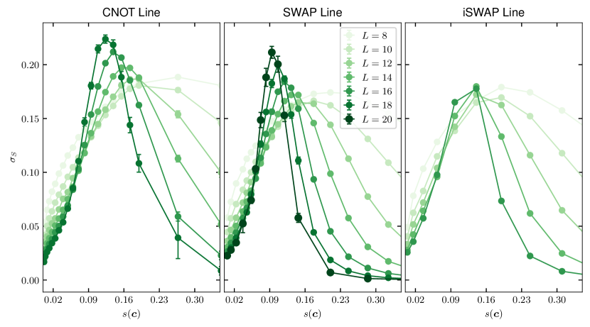
Figure 11: Entanglement entropy fluctuations $\sigma_{S}^{2}=\overline{s^{2}}-\overline{s}^{2}$ with $s=S/S_{\text{Page}}$ as function of the two-qubit gate operator entanglement. Right column: CNOT line denoted by $c_{1}\in[0.02,0.40]$. Middle column: SWAP line with $c_{1}\in[0.02,0.40]$. Left column: iSWAP line with $c_{1}\in[0.02,0.28]$. Error bars (too small for this scale) are $68\%$ confidence interval. The data set is the same shown in Fig.4 for $S/S_{\text{Page}}$.

It is known that fluctuations around the mean eigenstate entanglement entropy $\overline{S}$, probed by $\sigma_{S}^{2}=\overline{S^{2}}-\overline{S}^{2}$, peak at the transition point Luitz et al. (2015). Therefore tracking fluctuation’s peaks also reveals the possible location of the transition. Such fluctuations are shown in Fig. 11. We see that the peak of the fluctuations is moving towards smaller $s(\bm{c})$, as has been reported in other models where MBL might be stable Yu et al. (2016). Importantly, the entanglement entropy fluctuations also seem to be sensitive only to the operator entanglement $s(\bm{c})$ of the gate rather than the specific choice $(c_{1},c_{2},c_{3})$ in the Weyl chamber.

References

• Nandkishore and Huse (2015) Rahul Nandkishore and David A. Huse, “Many-Body Localization and Thermalization in Quantum Statistical Mechanics,” Annual Review of Condensed Matter Physics 6, 15–38 (2015).
• Abanin et al. (2019) Dmitry A. Abanin, Ehud Altman, Immanuel Bloch,  and Maksym Serbyn, “Colloquium: Many-body localization, thermalization, and entanglement,” Rev. Mod. Phys. 91, 021001 (2019).
• Ueda (2020) Masahito Ueda, “Quantum equilibration, thermalization and prethermalization in ultracold atoms,” Nat Rev Phys 2 (2020).
• Deutsch (1991) J. M. Deutsch, “Quantum statistical mechanics in a closed system,” Phys. Rev. A 43, 2046–2049 (1991).
• Srednicki (1994) Mark Srednicki, “Chaos and quantum thermalization,” Phys. Rev. E 50 (1994).
• Rigol et al. (2008) Marcos Rigol, Vanja Dunjko,  and Maxim Olshanii, “Thermalization and its mechanism for generic isolated quantum systems,” Nature 452 (2008).
• Heller (2001) Eric J. Heller, “Quantum Chaos: An Introduction,” Physics Today 54, 49–50 (2001).
• D’Alessio et al. (2016) Luca D’Alessio, Yariv Kafri, Anatoli Polkovnikov,  and Marcos Rigol, “From quantum chaos and eigenstate thermalization to statistical mechanics and thermodynamics,” Advances in Physics 65 (2016).
• Anderson (1958) P. W. Anderson, “Absence of Diffusion in Certain Random Lattices,” Phys. Rev. 109 (1958).
• Vidmar and Rigol (2016) Lev Vidmar and Marcos Rigol, “Generalized Gibbs ensemble in integrable lattice models,” J. Stat. Mech. 2016, 064007 (2016).
• Brenes et al. (2020) Marlon Brenes, Tyler LeBlond, John Goold,  and Marcos Rigol, “Eigenstate Thermalization in a Locally Perturbed Integrable System,” Phys. Rev. Lett. 125, 070605 (2020).
• Rigol (2016) Marcos Rigol, “Fundamental Asymmetry in Quenches Between Integrable and Nonintegrable Systems,” Phys. Rev. Lett. 116, 100601 (2016).
• Essler and Fagotti (2016) Fabian H. L. Essler and Maurizio Fagotti, “Quench dynamics and relaxation in isolated integrable quantum spin chains,” J. Stat. Mech. 2016, 064002 (2016).
• Rigol et al. (2007) Marcos Rigol, Vanja Dunjko, Vladimir Yurovsky,  and Maxim Olshanii, “Relaxation in a Completely Integrable Many-Body Quantum System: An Ab Initio Study of the Dynamics of the Highly Excited States of 1D Lattice Hard-Core Bosons,” Phys. Rev. Lett. 98, 050405 (2007).
• Basko et al. (2006) D. M. Basko, I. L. Aleiner,  and B. L. Altshuler, “Metal–insulator transition in a weakly interacting many-electron system with localized single-particle states,” Annals of Physics 321, 1126–1205 (2006).
• Gornyi et al. (2005) I. V. Gornyi, A. D. Mirlin,  and D. G. Polyakov, “Interacting Electrons in Disordered Wires: Anderson Localization and Low-$T$ Transport,” Phys. Rev. Lett. 95 (2005).
• Oganesyan and Huse (2007) Vadim Oganesyan and David A. Huse, “Localization of interacting fermions at high temperature,” Phys. Rev. B 75 (2007).
• Huse et al. (2014) David A. Huse, Rahul Nandkishore,  and Vadim Oganesyan, “Phenomenology of fully many-body-localized systems,” Phys. Rev. B 90, 174202 (2014).
• Serbyn et al. (2013) Maksym Serbyn, Z. Papić,  and Dmitry A. Abanin, “Local Conservation Laws and the Structure of the Many-Body Localized States,” Phys. Rev. Lett. 111, 127201 (2013).
• Schreiber et al. (2015) Michael Schreiber, Sean S. Hodgman, Pranjal Bordia, Henrik P. Lüschen, Mark H. Fischer, Ronen Vosk, Ehud Altman, Ulrich Schneider,  and Immanuel Bloch, “Observation of many-body localization of interacting fermions in a quasirandom optical lattice,” Science 349, 842–845 (2015).
• Luitz et al. (2015) David J. Luitz, Nicolas Laflorencie,  and Fabien Alet, “Many-body localization edge in the random-field Heisenberg chain,” Phys. Rev. B 91, 081103 (2015).
• Šuntajs et al. (2020) Jan Šuntajs, Janez Bonča, Tomaž Prosen,  and Lev Vidmar, “Quantum chaos challenges many-body localization,” Phys. Rev. E 102, 062144 (2020).
• Sels and Polkovnikov (2023) Dries Sels and Anatoli Polkovnikov, “Thermalization of Dilute Impurities in One-Dimensional Spin Chains,” Phys. Rev. X 13 (2023).
• Sels and Polkovnikov (2021) Dries Sels and Anatoli Polkovnikov, “Dynamical obstruction to localization in a disordered spin chain,” Phys. Rev. E 104 (2021).
• Kiefer-Emmanouilidis et al. (2021) Maximilian Kiefer-Emmanouilidis, Razmik Unanyan, Michael Fleischhauer,  and Jesko Sirker, “Slow delocalization of particles in many-body localized phases,” Phys. Rev. B 103 (2021).
• Morningstar et al. (2022) Alan Morningstar, Luis Colmenarez, Vedika Khemani, David J. Luitz,  and David A. Huse, “Avalanches and many-body resonances in many-body localized systems,” Phys. Rev. B 105 (2022).
• Sels (2022) Dries Sels, “Bath-induced delocalization in interacting disordered spin chains,” Phys. Rev. B 106 (2022).
• Crowley and Chandran (2020) P. J. D. Crowley and A. Chandran, “Avalanche induced coexisting localized and thermal regions in disordered chains,” Phys. Rev. Res. 2 (2020).
• Sierant and Zakrzewski (2022) Piotr Sierant and Jakub Zakrzewski, “Challenges to observation of many-body localization,” Phys. Rev. B 105, 224203 (2022).
• Sierant et al. (2020) Piotr Sierant, Dominique Delande,  and Jakub Zakrzewski, “Thouless Time Analysis of Anderson and Many-Body Localization Transitions,” Phys. Rev. Lett. 124 (2020).
• Panda et al. (2020) R. K. Panda, A. Scardicchio, M. Schulz, S. R. Taylor,  and M. Žnidarič, “Can we study the many-body localisation transition?” EPL 128, 67003 (2020).
• Crowley and Chandran (2022) Philip Crowley and Anushya Chandran, “A constructive theory of the numerically accessible many-body localized to thermal crossover,” SciPost Physics 12, 201 (2022).
• Laflorencie et al. (2022) Nicolas Laflorencie, Gabriel Lemarié,  and Nicolas Macé, “Topological order in random interacting Ising-Majorana chains stabilized by many-body localization,” Phys. Rev. Res. 4, L032016 (2022).
• De Roeck and Imbrie (2017) Wojciech De Roeck and John Z. Imbrie, “Many-body localization: stability and instability,” Philosophical Transactions of the Royal Society A: Mathematical, Physical and Engineering Sciences 375, 20160422 (2017).
• Thiery et al. (2018) Thimothée Thiery, François Huveneers, Markus Müller,  and Wojciech De Roeck, “Many-Body Delocalization as a Quantum Avalanche,” Phys. Rev. Lett. 121, 140601 (2018).
• Krajewski et al. (2022) B. Krajewski, L. Vidmar, J. Bonča,  and M. Mierzejewski, “Restoring Ergodicity in a Strongly Disordered Interacting Chain,” Phys. Rev. Lett. 129, 260601 (2022).
• Bulchandani et al. (2022) Vir B. Bulchandani, David A. Huse,  and Sarang Gopalakrishnan, “Onset of many-body quantum chaos due to breaking integrability,” Phys. Rev. B 105 (2022).
• Kraus and Cirac (2001) B. Kraus and J. I. Cirac, “Optimal creation of entanglement using a two-qubit gate,” Phys. Rev. A 63, 062309 (2001).
• Balakrishnan and Sankaranarayanan (2011a) S. Balakrishnan and R. Sankaranarayanan, “Measures of operator entanglement of two-qubit gates,” Phys. Rev. A 83, 062320 (2011a).
• Balakrishnan and Sankaranarayanan (2010) S. Balakrishnan and R. Sankaranarayanan, “Entangling power and local invariants of two-qubit gates,” Phys. Rev. A 82, 034301 (2010).
• Balakrishnan and Sankaranarayanan (2009) S. Balakrishnan and R. Sankaranarayanan, “Characterizing the geometrical edges of nonlocal two-qubit gates,” Phys. Rev. A 79, 052339 (2009).
• Zhang et al. (2003) Jun Zhang, Jiri Vala, Shankar Sastry,  and K. Birgitta Whaley, “Geometric theory of nonlocal two-qubit operations,” Phys. Rev. A 67, 042313 (2003).
• Makhlin (2002) Yuriy Makhlin, “Nonlocal Properties of Two-Qubit Gates and Mixed States, and the Optimization of Quantum Computations,” Quantum Information Processing 1, 243–252 (2002).
• Balakrishnan and Sankaranarayanan (2011b) S. Balakrishnan and R. Sankaranarayanan, “Operator-Schmidt decomposition and the geometrical edges of two-qubit gates,” Quantum Inf Process 10, 449–461 (2011b).
• Bertini et al. (2019a) Bruno Bertini, Pavel Kos,  and Tomaz Prosen, “Entanglement spreading in a minimal model of maximal many-body quantum chaos,” Phys. Rev. X 9, 021033 (2019a).
• Bertini and Piroli (2020) Bruno Bertini and Lorenzo Piroli, “Scrambling in random unitary circuits: Exact results,” Phys. Rev. B 102, 064305 (2020).
• Akila et al. (2016) M Akila, D Waltner, B Gutkin,  and T Guhr, “Particle-time duality in the kicked ising spin chain,” Journal of Physics A: Mathematical and Theoretical 49, 375101 (2016).
• Bensa and Žnidarič (2021) Jaš Bensa and Marko Žnidarič, “Fastest Local Entanglement Scrambler, Multistage Thermalization, and a Non-Hermitian Phantom,” Phys. Rev. X 11, 031019 (2021).
• Zhou and Harrow (2022) Tianci Zhou and Aram W. Harrow, “Maximal entanglement velocity implies dual unitarity,” Phys. Rev. B 106, L201104 (2022).
• Rampp et al. (2023) Michael A. Rampp, Roderich Moessner,  and Pieter W. Claeys, “From Dual Unitarity to Generic Quantum Operator Spreading,” Phys. Rev. Lett. 130, 130402 (2023).
• Bertini et al. (2019b) Bruno Bertini, Pavel Kos,  and Tomaž Prosen, “Exact Correlation Functions for Dual-Unitary Lattice Models in $1+1$ Dimensions,” Phys. Rev. Lett. 123, 210601 (2019b).
• Fisher et al. (2023) Matthew P.A. Fisher, Vedika Khemani, Adam Nahum,  and Sagar Vijay, “Random Quantum Circuits,” Annual Review of Condensed Matter Physics 14, 335–379 (2023).
• Piroli et al. (2020) Lorenzo Piroli, Bruno Bertini, J. Ignacio Cirac,  and Tomaž Prosen, “Exact dynamics in dual-unitary quantum circuits,” Phys. Rev. B 101, 094304 (2020).
• Bertini et al. (2020a) Bruno Bertini, Pavel Kos,  and Tomaž Prosen, “Operator Entanglement in Local Quantum Circuits I: Chaotic Dual-Unitary Circuits,” SciPost Physics 8, 067 (2020a).
• Bertini et al. (2020b) Bruno Bertini, Pavel Kos,  and Tomaž Prosen, “Operator Entanglement in Local Quantum Circuits II: Solitons in Chains of Qubits,” SciPost Physics 8, 068 (2020b).
• Claeys and Lamacraft (2021) Pieter W. Claeys and Austen Lamacraft, “Ergodic and Nonergodic Dual-Unitary Quantum Circuits with Arbitrary Local Hilbert Space Dimension,” Phys. Rev. Lett. 126, 100603 (2021).
• Aravinda et al. (2021) S. Aravinda, Suhail Ahmad Rather,  and Arul Lakshminarayan, “From dual-unitary to quantum Bernoulli circuits: Role of the entangling power in constructing a quantum ergodic hierarchy,” Phys. Rev. Res. 3, 043034 (2021).
• Bertini et al. (2021) Bruno Bertini, Pavel Kos,  and Tomaž Prosen, “Random Matrix Spectral Form Factor of Dual-Unitary Quantum Circuits,” Commun. Math. Phys. 387, 597–620 (2021).
• Bertini et al. (2018) Bruno Bertini, Pavel Kos,  and Tomaž Prosen, “Exact Spectral Form Factor in a Minimal Model of Many-Body Quantum Chaos,” Phys. Rev. Lett. 121, 264101 (2018).
• Borsi and Pozsgay (2022) Márton Borsi and Balázs Pozsgay, “Construction and the ergodicity properties of dual unitary quantum circuits,” Phys. Rev. B 106, 014302 (2022).
• Bertini et al. (2019c) Bruno Bertini, Pavel Kos,  and Tomaž Prosen, “Entanglement Spreading in a Minimal Model of Maximal Many-Body Quantum Chaos,” Phys. Rev. X 9, 021033 (2019c).
• Alet and Laflorencie (2018) Fabien Alet and Nicolas Laflorencie, “Many-body localization: An introduction and selected topics,” Comptes Rendus Physique 19, 498–525 (2018).
• Foxen et al. (2020) B. Foxen, C. Neill, A. Dunsworth, P. Roushan, B. Chiaro, A. Megrant, J. Kelly, Zijun Chen, K. Satzinger, R. Barends, F. Arute, K. Arya, R. Babbush, D. Bacon, J. C. Bardin, S. Boixo, D. Buell, B. Burkett, Yu Chen, R. Collins, E. Farhi, A. Fowler, C. Gidney, M. Giustina, R. Graff, M. Harrigan, T. Huang, S. V. Isakov, E. Jeffrey, Z. Jiang, D. Kafri, K. Kechedzhi, P. Klimov, A. Korotkov, F. Kostritsa, D. Landhuis, E. Lucero, J. McClean, M. McEwen, X. Mi, M. Mohseni, J. Y. Mutus, O. Naaman, M. Neeley, M. Niu, A. Petukhov, C. Quintana, N. Rubin, D. Sank, V. Smelyanskiy, A. Vainsencher, T. C. White, Z. Yao, P. Yeh, A. Zalcman, H. Neven,  and J. M. Martinis (Google AI Quantum), “Demonstrating a continuous set of two-qubit gates for near-term quantum algorithms,” Phys. Rev. Lett. 125, 120504 (2020).
• Garratt and Chalker (2021) S. J. Garratt and J. T. Chalker, “Many-body delocalization as symmetry breaking,” Phys. Rev. Lett. 127, 026802 (2021).
• Pal and Huse (2010) Arijeet Pal and David A. Huse, “Many-body localization phase transition,” Phys. Rev. B 82, 174411 (2010).
• Atas et al. (2013) Y. Y. Atas, E. Bogomolny, O. Giraud,  and G. Roux, “Distribution of the Ratio of Consecutive Level Spacings in Random Matrix Ensembles,” Phys. Rev. Lett. 110 (2013).
• Page (1993) Don N. Page, “Average entropy of a subsystem,” Phys. Rev. Lett. 71, 1291–1294 (1993).
• Khemani et al. (2017) Vedika Khemani, S. P. Lim, D. N. Sheng,  and David A. Huse, “Critical properties of the many-body localization transition,” Phys. Rev. X 7, 021013 (2017).
• Yu et al. (2016) Xiongjie Yu, David J. Luitz,  and Bryan K. Clark, “Bimodal entanglement entropy distribution in the many-body localization transition,” Phys. Rev. B 94 (2016).
• Luitz (2021) David J. Luitz, “Polynomial filter diagonalization of large Floquet unitary operators,” SciPost Physics 11, 021 (2021).
• Long et al. (2023) David M. Long, Philip J. D. Crowley, Vedika Khemani,  and Anushya Chandran, “Phenomenology of the prethermal many-body localized regime,” Phys. Rev. Lett. 131, 106301 (2023).
• Luitz et al. (2016) David J. Luitz, Nicolas Laflorencie,  and Fabien Alet, “Extended slow dynamical regime close to the many-body localization transition,” Phys. Rev. B 93, 060201 (2016).
• Lezama et al. (2019) Talía L. M. Lezama, Soumya Bera,  and Jens H. Bardarson, “Apparent slow dynamics in the ergodic phase of a driven many-body localized system without extensive conserved quantities,” Phys. Rev. B 99, 161106 (2019).
• Lezama et al. (2021) Talía L. M. Lezama, E. Jonathan Torres-Herrera, Francisco Pérez-Bernal, Yevgeny Bar Lev,  and Lea F. Santos, “Equilibration time in many-body quantum systems,” Phys. Rev. B 104, 085117 (2021).
• Žnidarič et al. (2008) Marko Žnidarič, Tomaž Prosen,  and Peter Prelovšek, “Many-body localization in the Heisenberg $XXZ$ magnet in a random field,” Phys. Rev. B 77, 064426 (2008).
• Kjäll et al. (2014) Jonas A. Kjäll, Jens H. Bardarson,  and Frank Pollmann, “Many-Body Localization in a Disordered Quantum Ising Chain,” Phys. Rev. Lett. 113, 107204 (2014).
• Bardarson et al. (2012) Jens H. Bardarson, Frank Pollmann,  and Joel E. Moore, “Unbounded Growth of Entanglement in Models of Many-Body Localization,” Phys. Rev. Lett. 109, 017202 (2012).
• Developers (2023) Cirq Developers, “Cirq,”  (2023), See full list of authors on Github: https://github .com/quantumlib/Cirq/graphs/contributors.
• Krajewski et al. (2023) B. Krajewski, L. Vidmar, J. Bonča,  and M. Mierzejewski, “Strongly disordered Anderson insulator chains with generic two-body interaction,” Phys. Rev. B 108, 064203 (2023).