Controlling Nonequilibrium Bose Condensation with Engineered Environments

Abstract

Out of thermal equilibrium, bosonic quantum systems can Bose-condense away from the ground state, featuring a macroscopic occupation of an excited state, or even of multiple states in the so-called Bose-selection scenario. While theory has been developed describing such effects as they result from the nonequilibrium kinetics of quantum jumps, a theoretical understanding, and the development of practical strategies, to control and drive the system into desired Bose condensation patterns have been lacking. We show how fine-tuned single or multiple condensate modes, including their relative occupation, can be engineered by coupling the system to artificial quantum baths. Moreover, we propose a Bose ‘condenser’, experimentally implementable in a superconducting circuit, where bath engineering is realized via auxiliary driven-damped two-level systems, that induces targeted Bose condensation into eigenstates of a chain of resonators. We further discuss the engineering of transition points between different Bose condensation configurations, which may find application for amplification, heat-flow control, and the design of highly-structured quantum baths.

Non-equilibrium Bose condensation (BC) beyond canonical lasers has been widely explored in experiments in different platforms [1], such as photons in dye-filled cavities [2, 3, 4, 5, 6, 7, 8], excitons [9, 10, 11] and exciton-polaritons [12, 13, 14, 15, 16, 17, 18, 19] in (cavity) semiconductor heterostructures. BC in these systems arises from the interplay of thermalization with pump and loss, and the condensate mode is primarily determined by the pumping-loss ratios. Non-equilibrium BC of a different kind is predicted to occur, however, also in the absence of pumping and loss, when other mechanisms deprive the ground-state of its privileged role. Examples are open systems subject to parametric time-periodic driving or to a strong competition between heating and cooling mechanisms [20, 21, 22, 23, 24]. Complex steady states, with multiple condensates in Bose-selected modes, arise in these systems from the nonequilibrium quantum-jump kinetics. While a theoretical description of such effects has been worked out [20, 21], approaches to harness and control tailored BC patterns have been lacking. This includes a lack of theoretical understanding as well as concrete proposals for experimentally implementing the required form of control. The possibility to realize and transition between different (fragmented) condensates on demand is appealing for the design of quantum signal amplifiers, programmable multimode emitters, artificial quantum baths with highly-structured spectral densities, heat-flow switches.

In this work, we bridge this gap by developing a method, and proposing a concrete implementation, for engineering tailored excited-state BC and Bose selection (BS) patterns via the coupling of the system to simple synthetic reservoirs. We further exemplify the possibility to program transition points between different BC scenarios, as a potential application for amplification and heat-flow control. The capability of a Bose-selected state to exchange sharp macroscopic energy packets with the surroundings makes them, moreover, interesting for their potential use as structured artificial baths.

Bose selection. The behaviour of a system of $N$ noninteracting bosons at large density, weakly coupled to an environment via energy-exchange processes, is well captured by the kinetic equations for the occupations $n_{i}$ of the $M$ single-particle stationary (or Floquet) states $\ket{j}$ [20, 21, 25],

$$\frac{dn_{i}}{dt}=\sum_{j=0}^{M-1}\big{[}R_{ij}n_{j}(1+n_{i})-R_{ji}n_{i}(1+n_{j})\big{]},$$ (1)

Here, the nonlinearity results from bosonic enhancement (stimulated emission), i.e., the dependence of the rate on the occupation of the state the particle jumps to. Equation (1) involves the single-particle quantum jump rates $R_{ij}$ from state $\ket{j}$ to state $\ket{i}$, which are induced by the environment. They are assumed here to realize a fully connected network, implying a unique steady state [20].

Familiar equilibrium BC is reproduced by Eq. (1) when the rates describe the coupling to a thermal reservoir at inverse temperature $\beta$, namely $R_{ji}/R_{ij}=\exp[-\beta(E_{i}-E_{j})]$, where $E_{j}$ are the single-particle energies. For generic nonequilibrium steady states, satisfying $dn_{i}/dt=0$, the system can undergo BS [20], a generalized form of condensation, where single or multiple states acquire a macroscopic occupation with increasing $N$, while the occupation of other states saturates [sketch in Fig. 1(a)]. Single-state selection occurs when the rate of particle inflow into a state $\ket{c}$ from any other state $\ket{j}$ overcomes escape rates, $R_{cj}>R_{jc}$, thus making $\ket{c}$ ‘ground-state-like’. This situation is different from lasing, where the excited-state occupation is rather stabilized by gain and loss, which are assumed to be absent in our system (except for weak losses, discussed later). For fragmented BS, the set $S$ of selected states $\ket{j}$ and their occupations are a complex result of the rates and the connectivity of the quantum-jump network encoded in the rate-asymmetry matrix $A=R-R^{T}$ [20, 21, 25, 26, 27]. Except for fine tuning, $S$ contains always an odd number of states. The matrix $A$ can be depicted as a directed graph, where the nodes represent the states and an edge is directed from the $j$th to the $i$th node if $A_{ij}>0$. BS is described by the existence of a unique BC vector $\bm{\nu}=[\bm{\nu}_{S},\bm{\nu}_{\bar{S}}]^{T}$, approximating the solution of Eq. (1) at large densities, which satisfies [20]

$$A_{\bar{S}S}\bm{\nu}_{S}<0,\quad A_{SS}\bm{\nu}_{S}=0,\quad\bm{\nu}_{\bar{S}}=0,\quad\bm{\nu}_{S}>0.$$ (2)

The subscripts $S$ and $\bar{S}$ indicate sets of indices labelling selected and depleted states, respectively, such that, for instance, $A_{\bar{S}S}$ denotes the off-diagonal matrix block of $A$ connecting states in $S$ to states in $\bar{S}$ and $A_{SS}$ is the diagonal matrix block containing the coupling between selected states. The (in)equalities in Eq. (2) apply element-wise to the vectors involved. These conditions are derived from Eq. (1) by applying a high-density expansion $n_{i}=\nu_{i}N+\sum_{\alpha=1}^{\infty}\nu_{i}^{(\alpha)}/N^{\alpha-1}$ and requiring that in leading order $n_{i}>0$. For the selected states this is the zeroth order, $n_{i}\simeq\nu_{i}N>0$, and for the non-selected states this is the first order given by $n_{i}\simeq\nu^{(1)}_{i}=-\sum_{j\in S}R_{ij}\nu_{j}/\sum_{j\in S}A_{ij}\nu_{j}>0$.

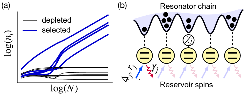
Figure 1: (a) Sketch of the BS effect: a subset of selected states acquires a macroscopic occupation with increasing particle number $N$, while the occupation of the other, depleted, states saturates. (b) Sketch of a ‘Bose condenser’: a resonator chain (blue-colored), where BC occurs in selected eigenmodes, is dispersively coupled to driven-damped reservoir two-level systems (yellow).

Control algorithm. Controlling BS requires engineering both the connectivity of quantum jumps in the network of states and their rate imbalance, as they enter the matrix $A$. This entails several challenges: developing concrete strategies to implement such a degree of incoherent control, identifying feasible rate networks mapping to desired BC patterns, efficiently determining the values of the control parameters to realize them. We find solutions to these challenges by designing a tuneable coupling of the system to a number $L$ of artificial baths. Each of these baths produces an asymmetry matrix $A^{(\ell)}$, determined by the corresponding engineered spectral density, such that the full matrix $A$ results as a linear combination

$$A=\sum_{\ell}z_{\ell}A^{(\ell)}.$$ (3)

The matrices $A^{(\ell)}$ constrain the quantum-jump connectivity, while the coupling variables $z_{\ell}\in\mathbb{R}$ (forming a vector $\bm{z}$) leverage the contribution of different baths and will be used as control parameters to enforce BC in a set $S$ with a desired target occupation $\bm{\nu}\geq 0$. For an open-system setup admitting a description as in Eq. (3), the BC-control problem can be reduced to that of finding solutions of certain linear inequalities for $\bm{z}$. Plugging Eq. (3) into (2) gives $\sum_{\ell}z_{\ell}A^{(\ell)}_{\bar{S}S}\bm{\nu}_{S}<0$ and $\sum_{\ell}z_{\ell}A^{(\ell)}_{SS}\bm{\nu}_{S}=0$, which can be rewritten as

$$\quad(B\bm{z})_{\bar{S}}<0,\quad(B\bm{z})_{S}=0\ .$$ (4)

The $M\times L$ matrix $B_{ij}\equiv\sum_{\ell\in S}A_{i\ell}^{(j)}\nu_{\ell}$ depends on the matrices $A^{(\ell)}$ and on the target Bose-selection vector $\bm{\nu}$. Solutions $\bm{z}$ of Eq. (4) will stabilize the desired steady state $\bm{\nu}$. They are found efficiently by means of linear-programming methods [28] [see Supplemental Material (SM) [29]], as is the case for the inequalities (2) [25]. This setup represents a powerful framework to reverse-engineer BS patterns. We next propose a physical system yielding rate-asymmetry matrices of the form of Eq. (3) and find couplings $\bm{z}$ giving desired single-state or fragmented BS.

Bose condenser. We consider an array of $M$ resonators representing the condensing system, each dispersively coupled to a two-level system (henceforth denoted “spin”), which is driven and strongly damped, as sketched in Fig. 1(b). This model can describe a chain of microwave resonators coupled to transmon qubits in a superconducting circuit [30, 31, 32, 33, 34, 35, 36]. The dynamics is described by the master equation ($\hbar=1$)

$$\frac{d\hat{\rho}}{dt}=-i[\hat{H}_{S}+\hat{H}_{B}+\hat{H}_{SB},\hat{\rho}]+\sum_{j}\gamma_{j}D[\hat{\sigma}_{j}^{-}]\hat{\rho},$$ (5)

for the density matrix $\hat{\rho}$ of the combined system, where $\gamma_{j}$ is the decay rate of the $\ell$th spin, $\hat{\sigma}_{j}^{\alpha}$ ($\alpha=x,y,z,\pm$) are Pauli matrices, and $D[\cdot]\hat{\rho}$ is a dissipator in Lindblad form [37]. The Hamiltonian $\hat{H}_{S}$ describes the free evolution of the bosonic system and is given by $\hat{H}_{S}=\sum_{j}\omega_{j}\hat{a}_{j}^{\dagger}\hat{a}_{j}-\sum_{i,j}J_{ij}\hat{a}_{i}^{\dagger}\hat{a}_{j},$ where $\hat{a}_{j}$ and $\hat{a}_{j}^{\dagger}$ are the annihilation and creation operators of a particle in the $j$th resonator, $\omega_{j}$ are the resonator transition frequencies and $J_{ij}>0$ is the tunnelling strength. The artificial-bath Hamiltonian $\hat{H}_{B}=\sum_{j}\delta_{j}\left(\hat{\sigma}^{z}_{j}+r_{j}\hat{\sigma}^{x}_{j}\right)/2$ describes the spins (in a frame rotating at the driving frequency), where $\delta_{j}$ is the detuning of the drive, and $r_{j}$ is the ratio between its Rabi frequency and $\delta_{j}$. The dispersive resonator-spin coupling is governed by $\hat{H}_{SB}=\sum_{j}\chi_{j}\hat{a}^{\dagger}_{j}\hat{a}_{j}\hat{\sigma}_{j}^{z}.$

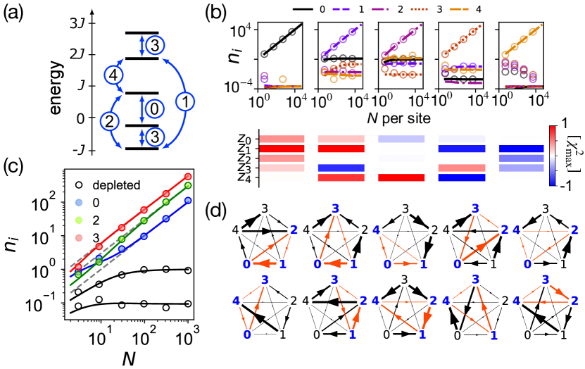
Figure 2: (a) Single-particle spectrum of the five-site chain. The numbers on the arrows indicate the reservoir spin associated to the related gap in the system. (b) Controlled BC into single modes, and corresponding values of the control parameters $\bm{z}/\chi^{2}_{\mathrm{max}}$ below (color scale). The lines are obtained from mean-field theory [Eq. (1)], while the bullets from $N_{t}=500$ trajectories (which thus grant enough resolution to faithfully reproduce occupations above $N_{t}^{-1}\sim 10^{-3}$, explaining deviations from mean field for strongly-depleted states). (c) BS with target occupation vector $\bm{\nu}=[1/10,0,3/10,6/10,0]$. Bullets, solid lines and dashed lines correspond to quasiexact method, mean-field and large-$N$ theory [Eq. (2)]. (d) Asymmetry matrices for BS in any triplet of modes (highlighted in blue). The arrow (red-coloured within $S$) thickness reflects the magnitude of the corresponding matrix element in arbitrary units.

We will consider the concrete example of $\hat{H}_{S}$ describing a 1D chain, with $J_{ij}=J$ for nearest neighbors $i$ and $j$, and each spin is used as an independent, narrow-band artificial bath. By appropriately choosing the driving parameters $\delta_{j}$ and $r_{j}$, the spin at level splitting $\mathcal{E}_{j}=\delta_{j}\sqrt{1+r_{j}^{2}}$ can resonate with a gap in the system, activating energy exchange without particle exchange. The strong spin damping quickly resets the spin to its (drive-dependent) steady state, such that the energy exchanged cannot be transferred back. The net effect on the bosonic chain is an incoherent state transfer. Whether this transfer involves energy absorption or emission is controlled by the sign of the detuning $\delta_{j}$. This reservoir engineering mechanism is akin to Raman-assisted cooling using cavity modes [38, 39, 40, 41]. However, the use of a nonlinear (two-level) element, rather than additional oscillators, as artificial bath is crucial here: the dispersive coupling to a damped resonator would simply reduce to a mutual state-independent energy shift [31], preventing dissipation engineering. To determine the rates $R_{ij}$, entering the kinetic Eqs. (1), from the microscopic master Eq. (5), we trace out the spins in favour of an effective spectral density [29]. This procedure, detailed in the SM [29], involves approximations relying on the conditions that $(i)$ the spins’ level splittings are much larger than their decay rates, $\mathcal{E}_{i}\gg\gamma_{i}$; $(ii)$ the system’s gaps are much larger than the system-‘bath’ effective couplings $|\chi_{ij}^{(\ell)}|$ and $|r_{\ell}\chi_{ij}^{(\ell)}|$, where $\chi_{ij}^{(\ell)}=r_{\ell}\chi_{\ell}M_{ij}^{(\ell)}/\sqrt{1+r_{\ell}^{2}}$ and $M_{ij}^{(\ell)}=\bra{i}\hat{a}_{\ell}^{\dagger}\hat{a}_{\ell}\ket{j}$; $(iii)$ the decay rates $\gamma_{i}$, while complying with $(i)$, are much larger than $|\chi_{ij}^{(\ell)}|$ and $|r_{\ell}\chi_{ij}^{(\ell)}|$. Condition $(i)$ ensures that a Markovian description of the spin decay remains justified under driving. Conditions $(ii)$ makes off-resonant system-spin energy transfer mechanisms negligible. Together with $(ii)$, condition $(iii)$ justifies a treatment of the spins within the Born-Markov approximation [37]: their state relaxes much quicker than the timescales of the system-spin coupling, and they thus behave effectively like a Markovian bath. The regime defined by $(i)$-$(iii)$ underpins the choice of parameters in the following examples, where the system gaps are of the order of a fixed tunnelling strength $J$, while $\gamma_{\ell}\in[J/10,J/5]$ and $|\chi_{ij}^{(\ell)}|<10^{-1}J$. It is important that the latter remains sizeable, since it influences the magnitude of the incoherent transition rates.

The rates induced by the $\ell$th spin bath resonating with the gap $E_{ij}\equiv E_{i}-E_{j}>0$, for $\delta_{\ell}>0$, are found to be

$$R^{(\ell)}_{ij}=\gamma_{-}^{(\ell)}|\chi_{ij}^{(\ell)}|^{2}\mathcal{S}_{\ell}(E_{ij}),\ R^{(\ell)}_{ji}=\gamma_{+}^{(\ell)}|\chi_{ij}^{(\ell)}|^{2}\mathcal{S}_{\ell}(E_{ij}),$$ (6)

where $\mathcal{S}_{\ell}(\omega)=2\Gamma_{\ell}/[(\omega-|\mathcal{E}_{\ell}|)^{2}+\Gamma_{\ell}^{2}]$ is a Lorentzian quantum-noise spectrum of linewidth $\Gamma_{\ell}=\gamma_{\ell}[3-1/(1+r_{\ell}^{2})]/4$. We introduced $\gamma_{\mp}^{(\ell)}=\sin^{4}[\theta_{\ell}+\Theta(\mp)\pi/2]/[\cos^{4}(\theta_{\ell})+\sin^{4}(\theta_{\ell})]$, with $\theta_{\ell}=\arctan(r_{\ell})/2$ and the Heaviside Theta function $\Theta(\cdot)$. For $\delta_{\ell}<0$, the rates have the same form (6), but with $\gamma^{(\ell)}_{\pm}$ exchanged. We verified that the rates (6) correctly reproduce the dynamics given by the full master Eq. (5) in the parameter regime considered [29].

For $\mathcal{E}_{\ell}\simeq E_{ij}>0$, the asymmetry matrix contributed by the rates (6) has the form $z_{\ell}A_{ij}^{(\ell)}$, with control variable $z_{\ell}=\chi_{\ell}^{2}[1-2\Theta(\delta_{\ell})]$ and

$$A_{ij}^{(\ell)}=\frac{8|M_{ij}^{(\ell)}|^{2}}{3+2r_{\ell}^{2}}\frac{\Gamma_{\ell}^{2}}{(E_{ij}-|\mathcal{E}_{\ell}|)^{2}+\Gamma_{\ell}^{2}}.$$ (7)

Assuming a fixed value of $r_{\ell}$, tuenability of $z_{\ell}$ implies control of the dispersive spin-resonator coupling $\chi_{\ell}$. This can be implemented by varying the detuning of the spin’s transition frequency from the bosonic chain [42, 31]. The sign of $\delta_{\ell}$ determines the sign of $z_{\ell}$ and thus controls whether the transition yields an energy increase or decrease in the system. The rate of the reversed process is suppressed with the ratio $R_{ij}^{(\ell)}/R_{ji}^{(\ell)}=\gamma_{-}^{(\ell)}/\gamma_{+}^{(\ell)}$ (for $\delta_{\ell}>0$). To guarantee experimental practicality of the protocols found, we restrict $\bm{z}$ to values $|z_{j}|/\chi^{2}_{\mathrm{max}}\in[0,1]$, such that the dispersive coupling is maintained below a maximal available value $\chi_{\mathrm{max}}$. An alternative formulation is possible and discussed in the SM [29]; there the control knob is the ratio $r_{\ell}$ of the spins’ drive parameters, while $\chi_{\ell}$ is kept fixed.

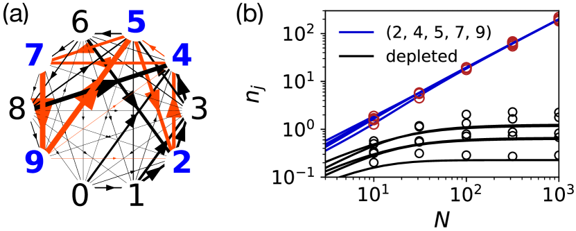
Figure 3: (a) Asymmetry matrix obtained for five-mode (blue-coloured) selection in a ten-site chain, with transitions within $S$ coloured in red. (b) Achievement of BS with requested equal occupancy. Solid lines indicate the result of mean field theory, while open circles represent the average results of 500 quasiexact quantum trajectories.

Programmable Bose condensates. With this setup, we exemplify BC control in a five-site chain, possessing the single-particle spectrum shown in Fig. 2(a). In the parameter regime complying with the assumptions discussed above, the specific choice of values is not crucial for the algorithm proposed to return effective condensation protocols, and the values used in the following examples are specified in the SM [29]. We first demonstrate controlled BC into a single arbitrary state. The energies of the reservoir spins are set in resonance with different gaps in the system, such that their effective spectral densities approximate the overall connectivity sketched in Fig. 2(a). Different gap-to-spin associations can be chosen, with the guiding principle of ensuring strong matrix elements $|M^{(\ell)}_{ij}|$, which is verified numerically. Control parameters $\bm{z}$ for each choice of selected state are found by solving the conditions (4). In Fig. 2(b) we show that condensation, indicated by a linear increase of the mode occupation with $N$, can be achieved in all five eigenmodes of the resonator chain. The steady state is computed using three different approaches: the kinetic equations (1) (solid lines), the asymptotic large-$N$ theory [Eq. (2)] (dashed lines), and the solution of the full master equation (bullets) from which Eq. (1) was derived [20, 21], capturing also non-trivial $n$-particle correlations. For the latter, we employed a quasi-exact quantum-trajectory-type unravelling [21].

We assumed until now negligible particle loss, namely that the resonators’ relaxation is much slower than the engineered dissipation. In the SM [29], we analyze the impact of weak particle leakage and propose a way to mitigate it through additional spin reservoirs realizing particle pumps. If the total mean particle number is kept large, we find that BS is still dictated by the matrix $A$ and is successfully controlled in the same manner as above. This is easily explained by the fact that BS is induced by the terms in Eq. (1) which are quadratic in the occupation numbers, while pump and loss still depend linearly on them (see, also, Ref. [6]). As an outlook, pump and loss may be used as additional control parameters.

We next control BS into a chosen set of three modes. We choose eigenstates $\{\ket{0},\ket{2},\ket{3}\}$ with target condensate fractions $[\bm{\nu}_{S,0},\bm{\nu}_{S,2},\bm{\nu}_{S,3}]=[1/10,3/10,6/10]$. The solution of Eq. (4) yields the desired BS pattern, depicted in Fig. 2(c). The occupations of selected states are proportional to $N$, while the non-selected-state occupations saturate. By exploring different connectivities through different gap-to-spin associations and solving for $\bm{z}$, protocols giving selection into any triplet of states, with the same occupation fractions as above, are found. The resulting asymmetry matrices for each triplet are shown in Fig. 2(d).

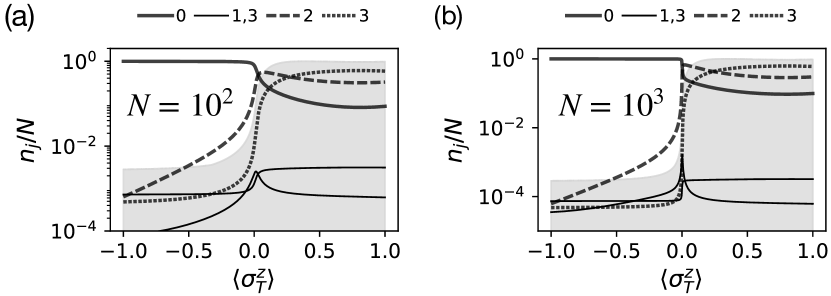
Figure 4: (a) BC pattern as a function of the expectation $\langle\hat{\sigma}_{T}^{z}\rangle$ of the ‘trigger’ spin, for $N=10^{2}$ (a) and $N=10^{3}$ (b). If $\langle\hat{\sigma}_{T}^{z}\rangle$ is negative, ground state BC occurs, whereas three-state selection is obtained for positive $\langle\hat{\sigma}_{T}^{z}\rangle$. The grey shading indicates the value of the heat $\mathcal{J}_{\ell}$ exchanged with the ‘positive temperature’ baths, renormalized by its maximal value. The transition, and the heat-flow difference, between the two BS patterns becomes sharper for larger $N$.

To exemplify controlled selection into more than three states, we target five modes of a ten-site chain. The reservoir spins realize rate asymmetries $A_{ij}$ for which each target mode is strongly connected to at least two other selected states. Choosing states $\{\ket{3},\ket{5},\ket{6},\ket{8},\ket{9}\}$ and solving Eqs (4) for $\bm{z}$, gives the asymmetry matrix of Fig. 3(a), and BS with chosen equal occupancy is successfully attained [Fig. 3(b)].

A condensate switch. The possibility to control different nonequilibrium phases which are per se robust, but tuned to be sensitive to few selected parameters, is a promising resource for applications in, e.g., amplification and sensing. Our framework allows one to tune the bosonic system to a parameter region in the vicinity of a transition between two (or more) BS configurations. The coupling to a trigger system can then determine which one is chosen depending on the state of the latter. Consider the five-site device of Fig. 2(a). If the quantum jump governed by the third spin is forced towards the ground state, the three-state BS breaks down in favour of ground state condensation. We can then picture a situation where the spin’s detuning $\delta_{3}$ is determined by the coupling to an additional trigger (‘$T$’) spin, as can be described by the spin-spin Hamiltonian $\hat{H}=\delta_{3}(r_{3}\hat{\sigma}_{3}^{x}+\hat{\sigma}_{3}^{z}\hat{\sigma}_{T}^{z})+\omega_{T}\hat{\sigma}_{T}^{z}/2$. Choosing the drive parameters such that $|\mathcal{E}_{3}|\approx|E_{20}|$, then the steady state of the bosonic chain will depend on the state of $`T^{\prime}$, through the renormalization of $\delta_{3}$ by $\langle\hat{\sigma}_{T}^{z}\rangle$. Depending whether $\langle\hat{\sigma}_{T}^{z}\rangle=\pm 1$, the chain will exhibit either three-state or ground-state selection, as numerically verified in Fig. 4(a).

The latter example can also be thought of as a switch for heat transport. Indeed, a BS phase accommodates a huge increase in steady-state heat flow through the system between the baths, compared to a single condensate [20]. This stems from the transition rate between selected states being bosonically-enhanced by the macroscopic occupation of both states. A dramatic increase of the heat flow into the ‘positive-temperature’ artificial baths can be observed when switching from one to three condensates [Fig. 4(a), shaded area], where the heat flow into the $\ell$th bath is defined as $\mathcal{J}_{\ell}=\sum_{ij}(E_{i}-E_{j})n_{i}(n_{j}+1)R^{(\ell)}_{ji}$.

Conclusion. We showed how Bose selection can be controlled via the coupling to engineered quantum baths. We designed a physical setup, implementable, e.g., in superconducting-circuit architectures, granting a handle on the condensate location and fragmentation, which can thus be shaped on demand. These results pave the way to applications in the control of heat transport, amplification, and quantum bath engineering. Combined with topologically non-trivial band structures, controlled selection may facilitate edge-mode detection [43], or realize topological-laser-like [44, 45] steady-states.

I Solving the inequalities for the control variables

As discussed in the main text, the existence of solutions $\bm{z}$ for the inequalities of Eq. (4) can be efficiently verified via linear programming. To this end, it is useful to recast the inequalities in a different but equivalent form. We start from the alternative formulation of the inequalities of Eq. (2) used in Refs. [25, 46]. Given the asymmetry matrix $A$ and the BC vector $\bm{\nu}$, the inequalities read

$$A\bm{\nu}\leq 0,\qquad(1-A)\bm{\nu}>0,\qquad\bm{\nu}\geq 0.$$ (S8)

We first show that these inequalities are indeed equivalent to the BS conditions of Eq. (2), which we restate here,

$$A_{SS}\bm{\nu}_{S}=0,\quad A_{\bar{S}S}\bm{\nu}_{S}<0,\quad\bm{\nu}_{S}>0,\quad\bm{\nu}_{\bar{S}}=0.$$ (S9)

Consider a solution of Eq. (S8). Since $\bm{\nu}\geq 0$, the entries of $\bm{\nu}$ can be divided into two sets, namely the set of non-zero entries $S=\{i:\nu_{i}>0\}$ and the set of vanishing entries $\bar{S}=\{i:\nu_{i}=0\}$. Identifying $S$ with the set of selected states, this gives the third and fourth condition in Eq. (S9). Accordingly, we decompose $\bm{\nu}=[\bm{\nu}_{S},\bm{\nu}_{\bar{S}}]=[\bm{\nu}_{S},\bm{0}]$ and the matrix $A$ gets decomposed into matrix blocks $\{A_{SS},A_{S\bar{S}},A_{\bar{S}S},A_{\bar{S}\bar{S}}\}$. Then, the system of inequalities (S8) gives the following conditions for the matrix blocks and $\bm{\nu}_{S}$,

$$A_{SS}\bm{\nu}_{S} \leq 0,$$

$$A_{\bar{S}S}\bm{\nu}_{S} <0,$$

$$\bm{\nu}_{S}-A_{SS}\bm{\nu}_{S} >0,$$

$$\bm{\nu}_{S} >0.$$ (S10)

The second inequality in (S10) is the same as the second inequality in (S9). We next note that, since $A_{SS}$ is skew-symmetric, its diagonal entries vanish and it thus follows that $\bm{\nu}_{S}^{T}A_{SS}\bm{\nu}_{S}=0$. However, the multiplication by the strictly positive $\bm{\nu}_{S}^{T}$ from the left-hand side cannot have changed the nature of the latter equality (e.g., turn an inequality into an equality), and it must hold that $A_{SS}\bm{\nu}_{S}=0$. The second condition in Eq. (S9) is then also recovered. This shows that the solution of Eq. (S8) fulfils the BS conditions (S9). The converse is obtained straightforwardly by noting that the solution of (S9) directly fulfils Eq. (S10).

Having shown that the inequalities (S8) are a different formulation of the BS conditions, we proceed as in the derivation of Eq. (4), by inserting the ansatz of Eq. (3) into Eq. (S8). We obtain the following inequalities for $\bm{z}$ at given target BC vector $\bm{\nu}\geq 0$,

$$B\bm{z}\leq 0,\quad B\bm{z}<\bm{\nu},$$ (S11)

where the matrix $B$ is defined as

$$B_{i\ell}=\sum_{j}A_{ij}^{(\ell)}\nu_{j}.$$ (S12)

These inequalities are equivalent to Eq. (4), but more amenable for numerical solution. Indeed, we can solve the system (S11) through linear programming routines by representing them as constraints to the linear program

$$\min_{\bm{z}}f(\bm{z})\quad\text{ subject to }\quad \mathcal{B}\bm{z}\leq\bm{n}_{\epsilon},$$

$$-z_{\rm max}\leq z_{j}\leq z_{\mathrm{max}},$$ (S13)

where $f(\bm{z})$ is a linear function of $\bm{z}$. While the usual goal of the linear program is to optimize the linear function $f(\bm{z})$ compatibly with the constraints, for our purposes it is sufficient to find a feasible solution satisfying the latter, and we can thus simply choose $f(\bm{z})=0$. The formulation of Eq. (I) is adopted for enabling the use of SciPy built-in routines [47]). In (I), we have defined the matrix $\mathcal{B}=[B,B]$ and the vector $\bm{n}_{\epsilon}=[\bm{0}_{\mathrm{dim}(B)},\bm{\nu}-\bm{\epsilon}]$, where $\bm{\epsilon}$ is a tolerance parameters with chosen value $\epsilon_{j}=10^{-2}$, allowing us to include the strict inequality of the second condition in (S11) as a ‘$\leq$’ inequality in (I). The constraint on $\bm{z}$ is imposed with $z_{\mathrm{max}}/\chi_{\rm max}^{2}=1$ to ensure experimental practicality of the parameters found, such that the dispersive coupling does not exceed a maximum value $\chi_{\rm max}$, as discussed in the main text.

II Reservoir engineering with driven-damped spins

In this section, the use of driven-damped spins as artificial reservoirs is discussed, and the single-particle transition rates are derived. To obtain a clear picture of the approximations involved, we will highlight and number them consecutively. We consider, for simplicity, a single reservoir spin coupled dispersively to the $\ell$-th resonator in the chain. The generalization to multiple reservoirs is straightforward, since in this case their individual rates will simply sum up. The spin is driven and subject to fast decay. The Hamiltonian, in a frame rotating at the driving frequency of the qubit, reads

$$\hat{H}=\hat{H}_{S}+\chi_{\ell}\hat{a}_{\ell}^{\dagger}\hat{a}_{\ell}\hat{\sigma}_{\ell}^{z}+\frac{\delta_{\ell}}{2}[\hat{\sigma}_{\ell}^{z}+r_{\ell}\hat{\sigma}_{\ell}^{x}],$$ (S14)

where $\delta_{\ell}$ is the spin-drive detuning, $r_{\ell}$ is the ratio between the Rabi frequency of the drive and its detuning, and $\hat{H}_{S}$ is the bosonic-chain Hamiltonian,

$$\hat{H}_{S}=\sum_{j=0}^{M-1}\omega_{j}\hat{a}_{j}^{\dagger}\hat{a}_{j}-J\sum_{j=0}^{M-2}(\hat{a}_{j}\hat{a}_{j+1}^{\dagger}+\hat{a}_{j}^{\dagger}\hat{a}_{j+1}).$$ (S15)

The dissipative dynamics of the system is described by the master equation

$$\frac{d\hat{\rho}}{dt}=-i[\hat{H},\hat{\rho}]+\gamma_{\ell}D[\hat{\sigma}_{\ell}^{-}]\hat{\rho},$$ (S16)

where $\gamma_{\ell}$ is the relaxation rate of the spin and $D[\cdot]\hat{\rho}$ is a Lindblad dissipator, $D[\cdot]\hat{\rho}=(\cdot)\hat{\rho}(\cdot)^{\dagger}-(1/2)\{(\cdot)^{\dagger}(\cdot),\,\hat{\rho}\}$. By diagonalizing the spin Hamiltonian via the unitary transformation $\hat{U}_{\ell}=-\sin(\theta_{\ell})\hat{\sigma}_{\ell}^{z}+\cos(\theta_{\ell})\hat{\sigma}_{\ell}^{x}$ with $\theta_{\ell}=\arctan(r_{\ell})/2$, one obtains

$$\hat{H}=\hat{H}_{S}-\frac{\delta_{\ell}\chi_{\ell}}{\mathcal{E}_{\ell}}\hat{a}_{\ell}^{\dagger}\hat{a}_{\ell}\big{[}\hat{\sigma}_{\ell}^{z}+r\hat{\sigma}_{\ell}^{x}\big{]}-\frac{\mathcal{E}_{\ell}}{2}\hat{\sigma}_{\ell}^{z},$$ (S17)

with $\mathcal{E}_{\ell}=\delta_{\ell}\sqrt{1+r_{\ell}^{2}}$. The transformation also affects the dissipator. It transforms as

$$\gamma_{\ell}D[\hat{U}_{\ell}^{\dagger}\hat{\sigma}_{\ell}^{-}\hat{U}_{\ell}]\hat{\rho}=\gamma_{\ell}\!\!\!\!\sum_{\begin{subarray}{c}\alpha,\beta\\ \in\{z,+,-\}\end{subarray}}\!\!\!\!K^{(\ell)}_{\alpha\beta}\big{(}\hat{\sigma}_{\ell}^{\alpha}\hat{\rho}\hat{\sigma}_{\ell}^{\beta}-\frac{1}{2}\{\hat{\sigma}_{\ell}^{\beta}\hat{\sigma}_{\ell}^{\alpha},\hat{\rho}\}\big{)}\ ,$$ (S18)

where the Kossakowski matrix $K^{(\ell)}$ reads

$$K^{(\ell)}=\begin{bmatrix}\frac{r_{\ell}^{2}}{4(1+r_{\ell}^{2})}&-\frac{r_{\ell}\cos^{2}\theta_{\ell}}{2(1+r_{\ell}^{2})}&\frac{r_{\ell}\sin^{2}\theta_{\ell}}{2(1+r_{\ell}^{2})}\\ -\frac{r_{\ell}\cos^{2}\theta_{\ell}}{2(1+r_{\ell}^{2})}&\cos^{4}\theta_{\ell}&\frac{r_{\ell}^{2}}{4(1+r_{\ell}^{2})}\\ \frac{r_{\ell}\sin^{2}\theta_{\ell}}{2(1+r_{\ell}^{2})}&-\frac{r_{\ell}^{2}}{4(1+r_{\ell}^{2})}&\sin^{4}\theta_{\ell}\end{bmatrix}\ .$$ (S19)

In the limit where the level splitting $|\mathcal{E}_{\ell}|$ of the spin is much larger than the decay rate $\gamma_{\ell}$, that is

$$|\mathcal{E}_{\ell}|\gg\gamma_{\ell},$$ (S20)

terms corresponding to off-diagonal elements of the Kossakowski matrix are off-resonant and can be neglected in rotating-wave approximation (RWA) (Approximation I). The transformed dissipator then reduces to

$$\gamma_{\ell}^{+}D[\hat{\sigma}_{\ell}^{+}]\hat{\rho}+\gamma_{\ell}^{-}D[\hat{\sigma}_{\ell}^{-}]\hat{\rho}+\gamma_{\ell}^{z}D[\hat{\sigma}_{\ell}^{z}]\hat{\rho},$$ (S21)

with dressed decay rates

$$\gamma_{\ell}^{+}=\gamma_{\ell}\cos^{4}(\theta_{\ell});\,\,\gamma_{\ell}^{-}=\gamma_{\ell}\sin^{4}(\theta_{\ell});\\ \gamma_{\ell}^{z}=\frac{\gamma_{\ell}}{4}\frac{r_{\ell}^{2}}{1+r_{\ell}^{2}}\ .$$ (S22)

When the spin level splitting $\mathcal{E}_{\ell}$ is in resonance with a gap in the system, and the spin decay rate is larger than the effective system-spin coupling, the spin can be traced out, yielding effective transition rates between the bosonic-chain eigenstates, ruled by a Lorentzian bath spectral density. To show this, we start by formally diagonalizing the bosonic chain, $\hat{H}_{S}=\sum_{j}E_{j}\hat{b}_{j}^{\dagger}\hat{b}_{j}$ with $\ket{j}=\hat{b}_{j}^{\dagger}\ket{v}$ the single-particle eigenstates and $\ket{v}$ the vacuum. In interaction picture with respect to the bare energies of the bosonic chain and spin, the Hamiltonian reads

$$\hat{H}(t)=-\sum_{i>j}\big{(}\chi^{(\ell)}_{ij}e^{iE_{ij}t}\hat{b}^{\dagger}_{i}\hat{b}_{j}+\chi^{(\ell)*}_{ij}e^{-iE_{ij}t}\hat{b}^{\dagger}_{j}\hat{b}_{i}\big{)}\\ \times\big{(}\frac{1}{r_{\ell}}\hat{\sigma}_{\ell}^{z}+e^{-i\mathcal{E}_{\ell}t}\hat{\sigma}_{\ell}^{+}+e^{i\mathcal{E}_{\ell}t}\hat{\sigma}_{\ell}^{-}\big{)},$$ (S23)

where $E_{ij}=E_{i}-E_{j}$, and

$$\chi^{(\ell)}_{ij}=\frac{\chi_{\ell}r_{\ell}M_{ij}^{(\ell)}}{\sqrt{1+r_{\ell}^{2}}},$$ (S24)

with matrix element $M_{ij}^{(\ell)}=\bra{i}\hat{a}_{\ell}^{\dagger}\hat{a}_{\ell}\ket{j}$. The dissipator remains unchanged. Consider now the case in which $\mathcal{E}_{\ell}\simeq E_{ij}>0$, namely the spin level splitting is (quasi)resonant with the gap $E_{ij}$. The terms $\hat{b}_{i}^{\dagger}\hat{b}_{j}\hat{\sigma}_{\ell}^{+}$ and $\hat{b}_{j}^{\dagger}\hat{b}_{i}\hat{\sigma}_{\ell}^{-}$ become resonant, and other terms can be neglected, in RWA, if the gap is much larger than the effective couplings (Approximation II),

$$E_{ij}\gg|\chi_{ij}^{(\ell)}|,\qquad E_{ij}\gg|r\chi_{ij}^{(\ell)}|\ .$$ (S25)

This yields the Schrödiger’s picture Hamiltonian (up to a constant energy shift)

$$\hat{H}= \frac{E_{ij}}{2}(\hat{b}_{i}^{\dagger}\hat{b}_{i}-\hat{b}_{j}^{\dagger}\hat{b}_{j})-\frac{\mathcal{E}_{\ell}}{2}\hat{\sigma}_{\ell}^{z}$$

$$-\sum_{(i,j)\mathrm{res}}\big{(}\chi^{(\ell)}_{ij}\hat{b}^{\dagger}_{i}\hat{b}_{j}\hat{\sigma}_{\ell}^{+}+\chi^{(\ell)*}_{ij}\hat{b}^{\dagger}_{j}\hat{b}_{i}\hat{\sigma}_{\ell}^{-}\big{)}.$$ (S26)

The summation runs over all pairs of single-particle eigenstates with gap quasiresonant with $\mathcal{E}_{\ell}$. For ease of notation, in the following we focus on a single such pair.

Next, we will trace out the spin, treating it as an environment degree of freedom, such that $\hat{H}$ of Eq. (S26) represents a system-bath coupling Hamiltonian. We proceed following standard Born-Markov-secular derivations [37]. The reason why this approach is justified, despite the spin being far from representing a true quantum bath, will be clarified in the following. The dynamics of the bosonic system is described by the Markovian quantum master equation for its density matrix $\hat{\rho}_{S}$ [37],

$$\frac{d\hat{\rho}_{S}}{dt}=\int_{0}^{+\infty}ds\ \mathrm{tr}_{\sigma}\big{[}\hat{H}(t),[\hat{H}(t-s),\hat{\rho}_{S}\otimes\hat{\rho}_{\sigma}]\big{]},$$ (S27)

where $\mathrm{tr}_{\sigma}$ and $\hat{\rho}_{\sigma}$ denote the trace over the degrees of freedom of the spin and the spin’s steady-state density matrix, respectively. $\hat{H}(t)$ represents the Hamiltonian of Eq. (S26) in the interaction picture. By adopting Eq. (S27), we are assuming the Born and Markov approximations (Approximation III). The latter are justified, if the spin state is negligibly affected by the coupling to the resonators, such that the states of these two systems can be approximated as factorised,

$$|\chi_{ij}^{(\ell)}|\ll|\mathcal{E}_{\ell}|\ .$$ (S28)

Moreover, the spin must relax quickly enough to its steady state, that its state can be considered as constant over the evolution timescales of the system. These conditions imply that the decay rate of the spin, $\gamma_{\ell}$, needs to be much stronger than the effective spin-resonator coupling entering the Hamiltonian (S26),

$$|\chi_{ij}^{(\ell)}|\ll\gamma_{\ell}\ .$$ (S29)

Note, however, that $\gamma_{\ell}$ needs also be small enough for Approximations I and II to be valid, and thus a hierarchical separation of energy scales between the level splittings, $\gamma_{\ell}$ and the effective system-spin coupling must be fulfilled.

Inserting Eq. (S26) into (S27) and following standard manipulations [37], the following master equation in the Lindblad form is obtained,

$$\frac{d\hat{\rho}_{S}}{dt}=R_{ij}^{(\ell)}D[\hat{b}^{\dagger}_{i}\hat{b}_{j}]\hat{\rho}_{S}+R_{ji}^{(\ell)}D[\hat{b}^{\dagger}_{j}\hat{b}_{i}]\hat{\rho}_{S}\ ,$$ (S30)

where Lamb-shift corrections have been neglected, and the rates $R_{ij}^{(\ell)}$ read

$$R^{(\ell)}_{ij}=|\chi_{ij}^{(\ell)}|^{2}\mathcal{S}_{\ell}^{+}(-E_{ij}),$$

$$R^{(\ell)}_{ji}=|\chi_{ij}^{(\ell)}|^{2}\mathcal{S}_{\ell}^{-}(E_{ij}),\quad(\mbox{for }\delta_{\ell}>0)$$ (S31)

The quantum noise spectra $\mathcal{S}_{\ell}^{\pm}(\omega)$ in Eq. (II) are defined by

$$\mathcal{S}_{\ell}^{\pm}(\omega) =\int_{-\infty}^{\infty}dte^{i\omega t}\langle[\hat{\sigma}_{\ell}^{\pm}(t)]^{\dagger}\hat{\sigma}_{\ell}^{\pm}(0)\rangle_{\sigma},$$

$$=2\mathrm{Re}\int_{0}^{\infty}dte^{i\omega t}\langle[\hat{\sigma}_{\ell}^{\pm}(t)]^{\dagger}\hat{\sigma}_{\ell}^{\pm}(0)\rangle_{\sigma}.$$ (S32)

Here, $\langle\cdot\rangle_{\sigma}=\mathrm{tr}[(\cdot)\rho_{\sigma}]$ indicates the average with respect to the spin’s steady state $\hat{\rho}_{\sigma}$. For negative times we have used the property $\langle[\sigma_{\ell}^{\pm}(-t)]^{\dagger}\sigma_{\ell}^{\pm}(0)\rangle_{\sigma}=\langle[\sigma_{\ell}^{\pm}(t)]^{\dagger}\sigma_{\ell}^{\pm}(0)\rangle_{\sigma}^{*}$. The time-dependent operators $\hat{\sigma}_{\ell}^{+}(t)$ are interaction picture representations of $\hat{\sigma}_{\ell}^{\pm}$. In deriving Eq. (S30), an additional secular approximation has been made to arrive at the Lindblad form, which is consistent with Approximation II. The master Eq. (S30) has been derived by assuming quasiresonance between $\mathcal{E}_{\ell}$ and $E_{ij}>0$, implying a positive detuning $\delta_{\ell}>0$. For negative detuning, the terms $\hat{b}_{i}^{\dagger}\hat{b}_{j}\hat{\sigma}_{\ell}^{-}$ and $\hat{b}_{j}^{\dagger}\hat{b}_{i}\hat{\sigma}_{\ell}^{+}$ in Eq. (S23) become resonant instead. In this case, the derivation of the master equation is the same as above, only with the role of $\hat{\sigma}_{\ell}^{-}$ and $\hat{\sigma}_{\ell}^{+}$ [and thus $\mathcal{S}_{\ell}^{-}(\omega)$ and $\mathcal{S}_{\ell}^{+}(\omega)$] exchanged, yielding rates

$$R^{(\ell)}_{ij}=|\chi_{ij}^{(\ell)}|^{2}\mathcal{S}_{\ell}^{-}(-E_{ij}),$$ (S33)

$$R^{(\ell)}_{ji}=|\chi_{ij}^{(\ell)}|^{2}\mathcal{S}_{\ell}^{+}(E_{ij}),\quad(\mbox{for }\delta_{\ell}<0).$$ (S34)

To explicitly compute the spectra (S32) entering the rates, the spin’s steady-state and correlation functions are needed. Consistently with the Markov approximation, we treat the spin as negligibly influenced by the coupling to the system, and compute such quantities as they are determined by free decay and coherent drive. This is achieved by solving the optical Bloch equations and using the quantum regression theorem [48, 37]. The problem is formally equivalent to that of a spontaneously decaying qubit with additional dephasing. The optical Bloch equations read

$$\frac{d}{dt}\begin{bmatrix}\langle\sigma_{\ell}^{z}\rangle(t)\\ \langle\sigma_{\ell}^{+}\rangle(t)\\ \langle\sigma_{\ell}^{-}\rangle(t)\\ \end{bmatrix}=\begin{bmatrix}-(\gamma_{\ell}^{+}+\gamma_{\ell}^{-})\langle\sigma_{\ell}^{z}\rangle(t)+\gamma_{\ell}^{+}-\gamma_{\ell}^{-}\\ (-i\mathcal{E}_{\ell}-\Gamma_{\ell})\langle\sigma_{\ell}^{+}\rangle(t)\\ (i\mathcal{E}_{\ell}-\Gamma_{\ell})\langle\sigma_{\ell}^{-}\rangle(t)\end{bmatrix},$$ (S35)

where

$$\Gamma_{\ell}=\frac{\gamma_{\ell}^{+}+\gamma_{\ell}^{-}}{2}+2\gamma_{\ell}^{z}=\frac{\gamma_{\ell}}{4}\left[3-\frac{1}{1+r_{\ell}^{2}}\right].$$ (S36)

The steady state $\hat{\rho}_{\sigma}$ thus satisfies

$$\langle\hat{\sigma}_{\ell}^{+}\rangle_{\sigma}=\langle\hat{\sigma}_{\ell}^{-}\rangle_{\sigma}=0,\qquad\langle\hat{\sigma}_{\ell}^{z}\rangle_{\sigma}=\frac{\gamma_{\ell}^{+}-\gamma_{\ell}^{-}}{\gamma_{\ell}^{+}+\gamma_{\ell}^{-}}.$$ (S37)

The steady state is thus fully depolarized in the dressed spin eigenbasis and the population imbalance of such eigenstates is ruled by

$$\langle\hat{\sigma}_{\ell}^{z}\rangle_{\sigma}=\frac{\gamma_{\ell}^{+}-\gamma_{\ell}^{-}}{\gamma_{\ell}^{+}+\gamma_{\ell}^{-}}=\frac{\sqrt{1+r_{\ell}^{2}}}{1+r_{\ell}^{2}/2}\ .$$ (S38)

From Eq. (S35) and the quantum regression theorem [48, 37], the relevant correlation functions are determined by

$$\frac{d}{dt}\langle[\sigma_{\ell}^{\pm}(t)]^{\dagger}\sigma_{\ell}^{\pm}(0)\rangle=(\pm i\mathcal{E}_{\ell}-\Gamma_{\ell})\langle[\sigma_{\ell}^{\pm}(t)]^{\dagger}\sigma_{\ell}^{\pm}(0)\rangle,$$ (S39)

and in the steady state they thus read

$$\langle\hat{\sigma}_{\ell}^{+}(t)\hat{\sigma}_{\ell}^{-}(0)\rangle_{\sigma}= e^{-(\Gamma_{\ell}+i\mathcal{E}_{\ell})t}\langle\hat{\sigma}_{\ell}^{+}(0)\hat{\sigma}_{\ell}^{-}(0)\rangle_{\sigma},$$

$$= \frac{\gamma_{\ell}^{+}}{\gamma_{\ell}^{+}+\gamma_{\ell}^{-}}e^{-(\Gamma_{\ell}+i\mathcal{E}_{\ell})t},$$ (S40)

$$\langle\hat{\sigma}_{\ell}^{-}(t)\hat{\sigma}_{\ell}^{+}(0)\rangle_{\sigma}= \frac{\gamma_{\ell}^{-}}{\gamma_{\ell}^{+}+\gamma_{\ell}^{-}}e^{-(\Gamma_{\ell}-i\mathcal{E}_{\ell})t}.$$ (S41)

Inserting into Eq. (S32) gives the Lorentzian quantum noise spectrum

$$\mathcal{S}_{\ell}^{\pm}(\omega)=\frac{\gamma_{\ell}^{\mp}}{\gamma_{\ell}^{+}+\gamma_{\ell}^{-}}\frac{2\Gamma_{\ell}}{(\omega\pm\mathcal{E}_{\ell})^{2}+\Gamma_{\ell}^{2}}.$$ (S42)

From Eq. (S42), one finds that $\mathcal{S}_{\ell}^{+}(-\omega)=(\gamma_{\ell}^{-}/\gamma_{\ell}^{+})\mathcal{S}_{\ell}^{-}(\omega)$, which indicates, together with Eq. (II) that the ratio $\gamma_{\ell}^{-}/\gamma_{\ell}^{+}$ controls the ratio between $j\rightarrow i$ and $j\leftarrow i$ transition rates. For a positive energy gap $E_{ij}>0$, the rates of Eq. (II) can thus be rewritten, using Eq. (S42), as

$$R_{ij}^{(\ell)}=|\chi_{ij}^{(\ell)}|^{2}[\gamma_{\ell}^{-}\Theta(\delta_{\ell})+\gamma_{\ell}^{+}\Theta(-\delta_{\ell})]\mathcal{S}_{\ell}(E_{ij}),$$ (S43a)

$$R_{ji}^{(\ell)}=|\chi_{ij}^{(\ell)}|^{2}[\gamma_{\ell}^{+}\Theta(\delta_{\ell})+\gamma_{\ell}^{-}\Theta(-\delta_{\ell})]\mathcal{S}_{\ell}(E_{ij}),$$ (S43b)

where $\Theta(\cdot)$ is Heaviside’s Theta function and

$$\mathcal{S}_{\ell}(\omega)=\frac{2\Gamma_{\ell}}{(\omega-|\mathcal{E}_{\ell}|)^{2}+\Gamma_{\ell}^{2}}.$$ (S44)

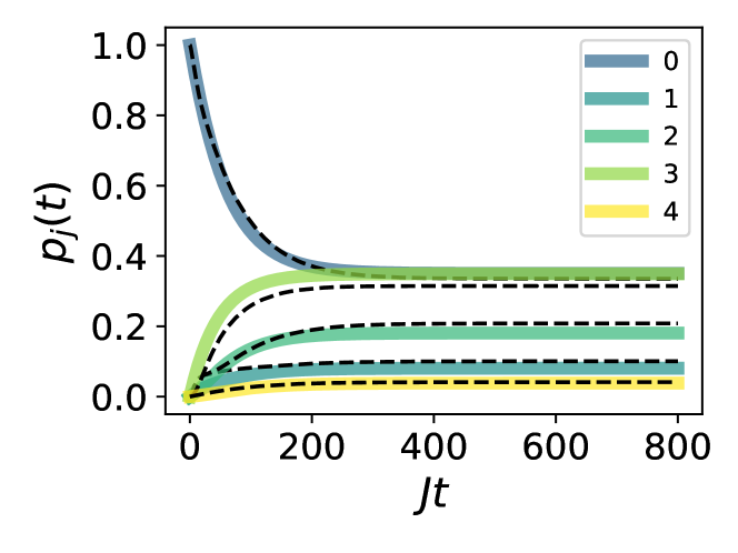
Figure S1: Comparison of the single-particle dynamics given by the effective rate equation for the resonator chain and the full resonators-spins master equation, Eq. (5), in terms of the time evolution of the occupation probabilities $p_{j}(t)$ of each eigenstate. The initial state is the bosonic-chain ground state. The rates used are those yielding the selection pattern of Fig. 2(c), and detailed in the next section.

We verify numerically that the expressions (S43a) and (S43b) for the rates correctly reproduce the dynamics given by the full master equation of Eq. (5), by comparing the single-particle evolution obtained with the two models. For the five-site chain discussed in the main text, including the coupling of a reservoir spin to each resonator, the evolution of the state populations is depicted in Fig. S1 for the system parameters producing the selection pattern of Fig. 2(c). One can appreciate that the two models produce essentially the same evolution, confirming the reliability of the rate model derived here.

The asymmetry matrix $A_{ij}^{(\ell)}=R_{ij}^{(\ell)}-R_{ji}^{(\ell)}$ produced by the rates (S43a) and (S43b) can be written in the form (for $i>j$)

$$A_{ij}^{(\ell)}=\chi_{\ell}^{2}[1-2\Theta(\delta_{\ell})]|M_{ij}^{(\ell)}|^{2}\mathcal{S}_{\mathrm{max}}(r_{\ell})L_{ij}^{(\ell)}(r_{\ell}),$$ (S45)

where we have introduced the function $\mathcal{S}_{\rm max}(r)$ describing the peak value as a function of $r$, and the function $0\leq L_{ij}^{(\ell)}(r)\leq 1$ containing the normalized Lorentzian enveloped. These functions explicitly read

$$\mathcal{S}_{\mathrm{max}}(r)=\frac{8r^{2}}{2+3r^{2}},$$ (S46)

$$L_{ij}^{(\ell)}(r)=\frac{\Gamma_{\ell}^{2}(r)}{[E_{ij}-|\delta_{\ell}|(1+r^{2})]^{2}+\Gamma_{\ell}^{2}(r)}.$$ (S47)

The functions $\mathcal{S}_{\mathrm{max}}(r)$, $\Gamma_{\ell}(r)$ and the product $\mathcal{S}_{\mathrm{max}}(r)L_{ij}^{(\ell)}(r)$ are shown in Fig. S2.

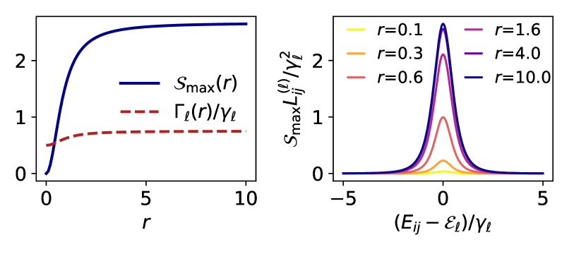
Figure S2: (a) Function $\mathcal{S}_{\mathrm{max}}(r)$ and linewidth $\Gamma_{\ell}(r)/\gamma_{\ell}$ of Eqs. (S46) and (S36) as a function of $r$. (b) Envelope $\mathcal{S}_{\mathrm{max}}(r)L^{(\ell)}_{ij}(r)$ of $A_{ij}^{(\ell)}$ [Eq. (S45),  (S46) and (S47)] for different values of $r$.

The asymmetry matrix of Eq. (S45) can be decomposed in the form $z_{\ell}A^{(\ell)}$, with a controllable prefactor $z_{\ell}$, in different ways:

1. One possible choice, adopted in the main text, is to assume a tuneable value of the dispersive coupling $\chi_{\ell}$, which can be achieved simply by varying the detuning of the spin’s transition frequency from the resonator chain, and a fixed ratio $r_{\ell}$ for the driving parameters on the spin. In particular the choice of decomposition is

   $$z_{\ell} =\chi_{\ell}^{2}[1-2\Theta(\delta_{\ell})],$$ (S48)

   $$A_{ij}^{(\ell)} =|M_{ij}^{(\ell)}|^{2}S_{\mathrm{max}}(r_{\ell})L^{(\ell)}_{ij}(r_{\ell}),$$ (S49)

   while $\chi_{\ell}$ determines the magnitude of the control parameter, $|z_{\ell}|=\chi_{\ell}^{2}$. The sign of $z_{\ell}$ is given by the sign of the detuning $\delta_{\ell}$. In the numerical simulations presented in main text, we used the fixed value $r_{\ell}=\mathrm{sgn}(\delta_{\ell})\sqrt{5}/2$.

2. For fixed resonator-spin couplings $\chi_{\ell}$, one can adapt the ratios $r_{\ell}$ between the driving parameters on the spins. Indeed, from Fig. (S2) one observes that the variation of the spectral linewidth $\Gamma_{\ell}(r)$ is small, as compared to the variation of the peak value $\mathcal{S}_{\mathrm{max}}(r)$. We may thus approximately treat $\Gamma_{\ell}(r)$ as constant and vary $r$ as control parameter, yielding the decomposition

   $$z_{\ell}=\mathcal{S}_{\mathrm{max}}(r_{\ell})[1-2\Theta(\delta_{\ell})],$$ (S50)

   $$A_{ij}^{(\ell)}=\chi_{\ell}^{2}|M_{ij}^{(\ell)}|^{2}L_{ij}^{(\ell)}(r_{\ell}).$$ (S51)

III Values of the parameters used in the simulations presented in the main text

Table S1: Values of $\chi_{\ell}$, in units of $\chi_{\mathrm{max}}$ and rounded to two significant digits, for the Bose-selection patterns in the five-site chain shown in Fig. 2(b)-(c).

$S$	$\chi_{0}$	$\chi_{1}$	$\chi_{2}$	$\chi_{3}$	$\chi_{4}$
{0, 1, 2}	1.0	0.71	0.88	0.97	0.86
{0}	0.66	1.0	0.64	0.43	0.12
{1}	0.48	1.0	0.0042	0.91	0.89
{2}	0.46	0.014	0.15	0.048	1.0
{3}	0.23	0.95	0.0031	0.68	1.0
{4}	0.067	1.0	0.72	0.59	0.084

In this section, the numerical values of the parameters used in the simulation producing the results shown in Figs. 2 and 3 are discussed. The frequencies $\omega_{j}$ of the bosonic chains are chosen freely, but in a way that avoids identical gaps in the spectrum. To this end we use, arbitrarily, $\omega_{j}/J=j/10+\varepsilon_{j}$, where $\varepsilon_{j}\in[0,1)$ is a disorder parameter picked from one realization of uniformly distributed random numbers, specifically $\bm{\varepsilon}=[0.55,0.73,0.60,0.54,0.42,0.65,0.44,0.89,0.96,0.38]$ (rounded to two significant digits). The resulting spectrum for the five-site chain is shown in Fig. 2(a). All reservoir spins decay with rate $\gamma_{\ell}/J=0.2$. The parameters $r_{\ell}$ are chosen as $r_{\ell}=\mathrm{sgn}(\delta_{\ell})\sqrt{5}/2$, where $\delta_{\ell}$ is fixed by (i) enforcing that the $\ell$th-spin level splitting $\mathcal{E}_{\ell}=|\delta_{\ell}|\sqrt{1+r_{\ell}^{2}}$ resonates with a chosen system gap $E_{ij}$ of the bosonic chain, and (ii) imposing the sign $\mathrm{sgn}(\delta_{\ell})$ found from the solution $\bm{z}$ of the inequalities of Eq. (4) for a given target condensation pattern. For the five-site chain with connectivity of Fig. 2(a), up to the sign of $\delta_{\ell}$ which depends on the choice of condensation patterns, the values used are then

$$|\delta_{0}|= 2E_{21}/3\simeq 0.65J,\quad |\delta_{3}|= 2E_{43}/3\simeq 0.51J,$$

$$|\delta_{1}|= 2E_{30}/3\simeq 1.8J,\quad |\delta_{4}|= 2E_{32}/3\simeq 0.69J,$$

$$|\delta_{2}|= 2E_{20}/3\simeq 1.11J.\quad$$ (S52)

The values of the dispersive couplings $\chi_{\ell}$, which are the physical control parameters leveraging the contribution of the different artificial baths to the total rate-asymmetry matrix, are obtained as $\chi_{\ell}=\sqrt{|z_{\ell}|}\chi_{\rm max}$ from the solution $\bm{z}$ of the Eq. (4), where we chose $\chi_{\rm max}/J=0.15$. For the single-state condensation of Fig. 2(b) and the three-state selection of Fig. 2(c), the values of $|z_{\ell}|$ are given in Table S1.

For the ten-site chain of Fig. 3, instead, the values of $\delta_{\ell}$ used are

$$|\delta_{0}|= 2E_{21}/3\simeq 0.21J, |\delta_{5}|=2E_{75}/3\simeq 0.87J,$$

$$|\delta_{1}|= 2E_{70}/3\simeq 2.3J, |\delta_{6}|=2E_{42}/3\simeq 0.73J,$$

$$|\delta_{2}|= 2E_{74}/3\simeq 1.2J, |\delta_{7}|=2E_{95}/3\simeq 7.1J,$$

$$|\delta_{3}|= 2E_{52}/3\simeq 1.1J, |\delta_{8}|=2E_{97}/3\simeq 6.2J,$$

$$|\delta_{4}|= 2E_{84}/3\simeq 2.0J, |\delta_{9}|=2E_{43}/3\simeq 0.41J.$$ (S53)

and the values of $\chi_{\ell}$ found are given in Table S2.

Table S2: Values of $\chi_{\ell}$, in units of $\chi_{\rm max}=0.15J$, corresponding to the ten-site selection pattern shown in Fig. 3.

$\chi_{0}$	$\chi_{1}$	$\chi_{2}$	$\chi_{3}$	$\chi_{4}$	$\chi_{5}$	$\chi_{6}$	$\chi_{7}$	$\chi_{8}$	$\chi_{9}$
0.94	0.24	0.79	1.0	1.0	0.93	0.85	0.91	1.0	0.24

IV Impact of pump and loss

We here discuss how particle pumping and loss from the resonators contribute to the mean-field equations, how they impact the Bose selection patterns, and how a pump for the resonators can be implemented.

In the presence of pumping and decay for each resonator, the master equation for the resonator chain reads

$$\frac{d\hat{\rho}}{dt}=-i[\hat{H}_{S},\hat{\rho}]+\sum_{j=1}^{M}(\kappa^{+}_{j}D[\hat{a}^{\dagger}_{j}]\hat{\rho}+\kappa_{j}^{-}D[\hat{a}_{j}]\hat{\rho}),$$ (S54)

where $\hat{H}_{S}$ is the chain Hamiltonian of Eq. (5) and $\kappa_{j}^{\pm}$ are the pump ($+$) and loss ($-$) rates for the $j$th resonator. For clarity, in Eq. (S54), we do not include the particle-number-conserving coupling to the artificial baths, whose contribution to the mean field equations can be treated separately, giving the terms in Eq. (1). Formally diagonalizing the Hamiltonian $\hat{H}_{S}=\sum_{j}E_{j}\hat{b}_{j}^{\dagger}\hat{b}_{j}$ through a transformation $\hat{b}_{j}=\sum_{i}V_{ji}\hat{a}_{i}$, the master equation in the chain eigenbasis reads

$$\frac{d\hat{\rho}}{dt}=-i[\hat{H}_{S},\hat{\rho}]+\sum_{j=1}^{M}\Big{(}\kappa^{+}_{j}D\big{[}\sum_{m}V_{mj}\hat{b}_{m}^{\dagger}\big{]}\hat{\rho}\\ +\kappa_{j}^{-}D\big{[}\sum_{m}V_{mj}^{*}\hat{b}_{m}\big{]}\hat{\rho}\Big{)}.$$ (S55)

Adopting the secular approximation [37], valid if the decay rates $\kappa_{j}^{\pm}$ are much smaller than the gaps in the system and their difference, Eq. (S55) reduces to

$$\frac{d\hat{\rho}}{dt}=-i[\hat{H}_{S},\hat{\rho}]+\sum_{m}(K_{m}^{+}D[\hat{b}_{m}^{\dagger}]\hat{\rho}+K_{m}^{-}D[\hat{b}_{m}]\hat{\rho}),$$ (S56)

with modified decay rates $K_{m}^{\pm}=\sum_{j=1}^{M}\kappa^{\pm}_{j}|V_{mj}|^{2}.$ Considering the mean occupation $n_{j}(t)=\mathrm{tr}[\hat{\rho}(t)\hat{n}_{j}]$ of the $j$th eigenstate, this yields in turn

$$\frac{dn_{j}(t)}{dt}=K_{j}^{+}(n_{j}+1)-K_{j}^{-}n_{j}.$$ (S57)

The terms on the r.h.s. of Eq. (S57) are then the pump-loss contribution to the mean-field equations to be included in Eq. (1). From the latter, the total steady-state particle number $N=\sum_{j}n_{j}$ in the system can be estimated by summing over $j$,

$$0 =\sum_{j}(K_{j}^{+}-K_{j}^{-})n_{j}+\sum_{j}K_{j}^{+},$$ (S58)

$$<N\mathrm{max}_{j}(K_{j}^{+}-K_{j}^{-})+\sum_{j}K_{j}^{+},$$ (S59)

which gives the estimate

$$N>\frac{\sum_{j}K_{j}^{+}}{\mathrm{max}_{j}(K_{j}^{-}-K_{j}^{+})}\ .$$ (S60)

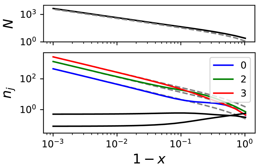
Figure S3: Bose selection in the five-site chain with pump and loss, as a function of the imbalance between pump and loss rates (lower panel). The latter are chosen as $K_{i}^{-}=R_{i}\times 0.1J$ and $K_{i}^{+}=(1-x)K_{i}^{-}$ where $R_{i},R_{i}^{\prime}$ are random numbers distributed uniformly in $[0,1)$. The mean steady-state total number of particles $N$ is depicted in the upper panel (solid line), where the dashed line shows the analytically predicted bound of Eq. (S60).

We analyze in Fig. S3 the fate of the Bose selection pattern obtained for the five-site chain of Fig. 2(c) when subject to pumping and loss with rates ratio $K_{i}^{+}/K_{i}^{-}=1-x$ for variable $x$. From the lower panel of Fig. S3, one can see that Bose condensation as predicted is indeed quickly attained as the pump rates approach the loss rates, and that the total mean number of particles increases accordingly [upper panel of Fig. S3]. The set of selected states is the one dictated by the controlled asymmetry matrix $A$, as predicted. Selection in the desired states is immediately attained also for weak pumping, and the chosen relative occupations are also recovered when the pump rates reach about 90$\%$ of the loss rates, confirming that Bose selection can successfully be controlled also for a leaky system.

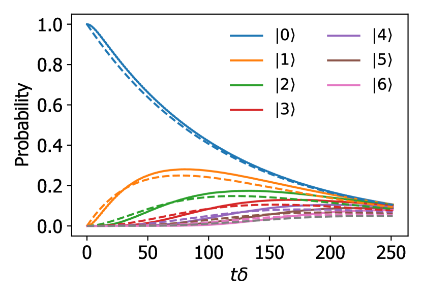
Figure S4: Probability of being in the different Fock states of the oscillator, with spin and oscillator initialized in their ground state. Solid lines are obtained by solving the master equation (S62), while dotted lines are obtained by the dissipator $\kappa^{+}D[a^{\dagger}]\rho$ with the predicted effective rate $\kappa^{+}=g^{2}/\gamma$. The parameter values used are $g=0.06\delta$, $\gamma=0.4\delta$.

We next discuss how to engineer a pump for the resonators, namely the terms $\kappa^{+}_{j}D[a^{\dagger}_{j}]\rho$ of Eq. (S54). We consider an auxiliary spin coupled in resonance to a resonator with a tuneable coupling $g(t)$. The Hamiltonian reads

$$\hat{H}(t)=\frac{\delta}{2}\hat{\sigma}_{z}+g(t)(\hat{\sigma}_{+}+\hat{\sigma}_{-})(\hat{a}+\hat{a}^{\dagger})+\delta\hat{a}^{\dagger}\hat{a},$$ (S61)

with $\delta\gg g(t)$. The spin is further strongly decaying with rate $g(t)\ll\gamma\ll\delta$, such that the qubit-oscillator master equation reads

$$\frac{d\hat{\rho}}{dt}=-i[\hat{H}(t),\hat{\rho}]+\gamma D[\hat{\sigma}_{-}]\hat{\rho}\ .$$ (S62)

We consider a drive of the coupling, of the form $g(t)=g\cos(2\delta t)$, which makes resonant counter-rotating terms $\hat{a}^{\dagger}\hat{\sigma}_{+}$ and $\hat{a}\hat{\sigma}_{-}$, such that, in interaction picture with respect to the bare Hamiltonians and in rotating wave approximation, the Hamiltonian becomes

$$H=\frac{g}{2}(\hat{\sigma}_{+}\hat{a}^{\dagger}+\hat{\sigma}_{-}\hat{a}).$$ (S63)

Because of the strong damping, only processes induced by $\hat{a}^{\dagger}\hat{\sigma}_{+}$ can effectively take place, followed by a quick resetting of the spin to the de-excited state, thus pumping the resonator. We can apply the results of previous sections, in particular the results discussed starting from Eq. (S23) for $\delta_{\ell}=0$. The transition rates between two oscillator states $\ket{n}$ and $\ket{n+1}$ read

$$R_{n+1,n} =\left(\frac{g}{2}\right)^{2}|\!\bra{n+1}\hat{a}^{\dagger}\ket{n}\!|^{2}S(0)$$ (S64)

$$=g^{2}(n+1)\mathcal{S}(0)/4,$$ (S65)

where $\mathcal{S}(\omega)$ is the spectral density

$$\mathcal{S}(\omega)=\frac{\gamma}{\omega^{2}+(\gamma/2)^{2}}.$$ (S66)

Due to the harmonicity of the oscillator, the spin drives all $\ket{n}\to\ket{n+1}$ transitions simultaneously, realizing the desired pump with a resonant pump rate $\kappa^{+}=g^{2}/\gamma$. The achievement of a pump as predicted is verified in Fig. S4, where the oscillator evolution produced by the master Eq. (S62) is compared with that given by the effective pump master equation $d\hat{\rho}/dt=\omega\hat{a}^{\dagger}\hat{a}+\kappa^{+}D[\hat{a}^{\dagger}]$.