Ly$\alpha$NNA: A Deep Learning Field-level Inference Machine for the Lyman-$\alpha$ Forest

The inference of astrophysical and cosmological properties from the Lyman-$\alpha$ forest conventionally relies on summary statistics of the transmission field that carry useful but limited information. We present a deep learning framework for inference from the Lyman-$\alpha$ forest at field-level. This framework consists of a 1D residual convolutional neural network (ResNet) that extracts spectral features and performs regression on thermal parameters of the IGM that characterize the power-law temperature-density relation. We train this supervised machinery using a large set of mock absorption spectra from nyx hydrodynamic simulations at $z=2.2$ with a range of thermal parameter combinations (labels). We employ Bayesian optimization to find an optimal set of hyperparameters for our network, and then employ a committee of ten neural networks for increased statistical robustness of the network inference. In addition to the parameter point predictions, our machine also provides a self-consistent estimate of their covariance matrix with which we construct a pipeline for inferring the posterior distribution of the parameters. We compare the results of our framework with the traditional summary (PDF and power spectrum of transmission) based approach in terms of the area of the 68% credibility regions as our figure of merit (FoM). In our study of the information content of perfect (noise- and systematics-free) Ly$\alpha$ forest spectral data-sets, we find a significant tightening of the posterior constraints — factors of 5.65 and 1.71 in FoM over power spectrum only and jointly with PDF, respectively — that is the consequence of recovering the relevant parts of information that are not carried by the classical summary statistics.

1 Introduction

The characteristic arrangement of Ly$\alpha$ absorption lines in the spectra of distant quasars, commonly known as the “Ly$\alpha$ forest” (Lynds, 1971), has been shown to be a unique probe of the physics of the Universe at play over a wide window of cosmic history ($z\lesssim 6$). As the continua of emission by the quasars traverse the diffuse intergalactic gas, resonant scattering by the neutral Hydrogen leads to a net absorption of the radiation at the wavelength of the Ly$\alpha$ transition (Gunn & Peterson, 1965). In an expanding Universe where spectral redshift $z$ is a proxy of distance, a congregation of absorber clouds in the intergalactic medium (IGM) along a quasar sightline imprints a dense forest of Ly$\alpha$ absorption lines on their spectra. Due to cosmic reionization of Hydrogen being largely complete by $z\sim 6$ (e.g. McGreer et al. 2015), its neutral fraction $x_{{H\textsc{i}}}$ within the IGM is extremely minute, yet sufficient to produce this unique feature that enables a continuous trace of the cosmic gas.

The observations of the Ly$\alpha$ forest, through the advent of high-resolution instruments (e.g. Keck/HIRES and VLT/UVES) as well as large-scale structure surveys (e.g. eBOSS (Dawson et al., 2013) and DESI (DESI Collaboration et al., 2022)), have delivered a wealth of information about the nonlinear matter distribution on sub-Mpc scales, thermal properties of the intergalactic gas, and large scale structure. Not only is the Ly$\alpha$ forest an extremely useful tool to study the thermal evolution of the intergalactic medium (IGM) and reionization (as demonstrated, e.g., by Becker et al. 2011, Walther et al. 2019, Boera et al. 2019, Gaikwad et al. 2021), but it has also opened up avenues for constraining fundamental cosmic physics. Chief among those are baryonic acoustic oscillations (BAO) and cosmic expansion (e.g., Slosar et al. 2013, Busca et al. 2013, du Mas des Bourboux et al. 2020, Gordon et al. 2023, Cuceu et al. 2023) , the nature and properties of dark matter (e.g., Viel et al. 2005, Viel et al. 2013, Iršič et al. 2017, Armengaud et al. 2017, Rogers & Peiris 2021) and in combination with the cosmic microwave background (CMB, e.g. Planck Collaboration et al. 2020) also inflation and neutrino masses (e.g., Seljak et al. 2006, Palanque-Delabrouille et al. 2015, Yèche et al. 2017, Palanque-Delabrouille et al. 2020).

The classical way of doing parameter inference with the Ly$\alpha$ forest, as for any other cosmic tracer, relies on summary statistics of the underlying field, as they conveniently pick out a small number of relevant features from a much larger number of degrees of freedom of the full data. For the Ly$\alpha$ forest, a number of summary statistics exists that have been accurately measured and effectively used for cosmological and astrophysical parameter inference. These include the line-of-sight (1D) transmission power spectrum (TPS hereinafter; e.g., Croft et al. 1998, Chabanier et al. 2019, Walther et al. 2019, Boera et al. 2019, Ravoux et al. 2023, Karaçaylı et al. 2023), transmission PDF (TPDF hereinafter; e.g., McDonald et al. 2000, Bolton et al. 2008, Viel et al. 2009, Lee et al. 2015), wavelet statistics (e.g., Meiksin 2000, Theuns & Zaroubi 2000, Zaldarriaga 2002, Lidz et al. 2010, Wolfson et al. 2021), curvature statistics (e.g., Becker et al. 2011, Boera et al. 2014), distributions of absorption line fits (e.g., Schaye et al. 2000, Bolton et al. 2014, Hiss et al. 2019, Telikova et al. 2019, Hu et al. 2022) and combinations thereof (e.g., Garzilli et al. 2012, Gaikwad et al. 2021). While these provide accurate measurements of parameter values, they fail to capture the full information contained in the transmission field, thereby resulting in a loss of constraining power the full spectral data-sets have to offer.

Recently, deep learning approaches have become popular in the context of cosmological simulations and data analysis. Complex and resource-heavy conventional problems in cosmology have started to see fast, efficient, and demonstrably robust solutions in neural network (NN) based algorithms (see, e.g., Moriwaki et al. 2023 for a recent review). Artificial intelligence has opened up a broad avenue for studies of the Ly$\alpha$ forest as well. Cosmological analyses with the Ly$\alpha$ forest generally demand expensive hydrodynamic simulations for an accurate modeling of the small-scale physics of the IGM. Deep learning offers alternative, light-weight solutions to such problems. For instance, Harrington et al. (2022) and Boonkongkird et al. (2023) recently built U-Net based frameworks for directly predicting hydrodynamic quantities of the gas from computationally much less demanding, dark-matter-only simulations. A super-resolution generative model of Ly$\alpha$-relevant hydrodynamic quantities is presented in Jacobus et al. (2023), based on conditional generative adversarial networks (cGANs). These works greatly accelerate the generation of mock data for Ly$\alpha$ forest analyses. Deep learning is also demonstrated to be a very effective methodology for a variety of tasks involving spectral, one-dimensional data-sets. Ďurovčíková et al. (2020) introduced a deep NN to reconstruct high-$z$ quasar spectra containing Ly$\alpha$ damping wings. Melchior et al. (2022) and Liang et al. (2023) describe a framework for generating, analysing, reconstructing and detecting outliers from SDSS galaxy spectra that consists of an autoencoder and a normalizing flow architecture. Recent works have shown immense potential of various deep NN methods for the analysis of the Ly$\alpha$ forest. For example, a convolutional neural network (CNN) model to detect and characterize damped Ly$\alpha$ systems (DLAs) in quasar spectra was introduced by Parks et al. (2018). Similarly, Busca & Balland (2018) applied a deep CNN called “QuasarNET” for the identification (classification) and redshift-estimation of quasar spectra. Huang et al. (2021) constructed a deep learning framework to recover Ly$\alpha$ optical depth from noisy and saturated Ly$\alpha$ forest transmission. Later, Wang et al. (2022) applied the same idea to the reconstruction of the line-of-sight temperature of the IGM and detection of temperature discontinuities (e.g., hot bubbles). In neighbouring disciplines, deep learning is already identified as a reliable tool for field-level inference. For instance, a set of recent works (Gupta et al. 2018, Fluri et al. 2018, Ribli et al. 2019, Kacprzak & Fluri 2022 among others) has established the superiority of deep learning techniques for cosmological inference directly from weak gravitational lensing maps over the classical two-point statistics of the cosmic density-field proxies.

In this work we present Ly$\alpha$NNA – short for “Ly$\alpha$ Neural Network Analysis” – a deep learning framework for the analysis of the Ly$\alpha$ forest. Here, we have implemented a 1D ResNet (a special type of CNN with skip-connections between different convolutional layers to learn the residual maps; He et al. 2015a) called “Sansa” for inference of model parameters with Ly$\alpha$ forest spectral data-sets, harvesting the full information carried by the transmission field. We perform non-linear regression on the thermal parameters of the IGM directly from the spectra containing the Ly$\alpha$ forest absorption features that are extracted efficiently by our deep model. This architecture is trained in a supervised fashion using a large set of mock spectra from cosmological hydrodynamic simulations with known parameter labels to not only distinguish between two distinct parameter combinations but also pinpoint the exact location of a given spectral set in the parameter space. For better statistical reliability of our results, we employ a committee of ten neural networks for the inference, combining the outputs via bootstrap aggregation (Breiman, 2004). Finally, we build a likelihood model to perform inference on mock data-sets via Markov chain Monte Carlo (MCMC) and compare with classical summary statistics, namely a combination of TPS and TPDF, showcasing the improvement we gain by working at the field-level.

This paper is structured as follows. Section 2 describes the simulations, the mock Ly$\alpha$ forest spectra we use for training and testing our methodology, and the summary statistics we compare to. In Section 3 we introduce the inference framework of Sansa with details of the architecture and its training. Our results of doing inference with Sansa and a comparison with the traditional summary statistics are presented and discussed in Section 4. We conclude in Section 5 with a précis of our findings and an outlook.

2 Simulations

In this section we introduce the hydrodynamic simulation used throughout this work as well as the post-processing approach we adopt to generate mock Ly$\alpha$ forest spectra.

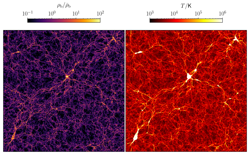
Figure 1: A slice (29 kpc thick) through our nyx simulation box (120 Mpc side-length, 4096 cells along a side) at $z=2.2$ shown here for the gas overdensity (left) and temperature (right). A systematic relationship between both the hydrodynamic fields can be seen.

2.1 Hydrodynamic Simulations

We use a nyx cosmological hydrodynamical simulation snapshot generated for Ly$\alpha$ forest analyses (see Walther et al. 2021) to create the mock data used for various purposes in this work. nyx is a relatively novel hydrodynamics code based on the AMReX framework and simulates an ideal gas on an Eulerian mesh interacting with dark matter modeled as Lagrangian particles. While adaptive mesh refinement (AMR) is possible and would allow better treatment of overdense regions, we used a uniform grid here as the Ly$\alpha$ forest only traces mildly overdense gas, rendering AMR techniques inefficient. Gas evolution is followed using a second-order accurate scheme (see Almgren et al. 2013 and Lukić et al. 2015 for more details). In addition to solving the Euler equations and gravity, nyx also models the main physical processes required for an accurate model of the Ly$\alpha$ forest. The chemistry of the gas is modeled following a primordial composition of H and He. Inverse Compton cooling of the CMB is taken into account as well as the updated recombination, collisional ionization, dielectric recombination and cooling rates from Lukić et al. (2015). All cells are assumed to be optically thin to ionizing radiation and a spatially uniform ultraviolet background (UVB) is applied according to the late reionization model of Oñorbe et al. (2017), where heating rates have been modified by a fixed factor $A_{\text{UVB}}$ affecting the thermal history and thus pressure smoothing of the gas.

Here, we use a simulation box at $z=2.2$ with 120 Mpc side-length and $4096^{3}$ volumetric cells (“voxels”) and dark matter particles, as motivated by recent convergence analyses (Walther et al. 2021 and Chabanier et al. 2023). The cosmological parameters of the box are $h=0.7035$, $\omega_{\text{m}}=\Omega_{\text{m}}h^{2}=0.1589$, $\omega_{\text{b}}=\Omega_{\text{b}}h^{2}=0.0223$, $A_{\mathrm{s}}=1.4258$, $n_{\mathrm{s}}=1.0327$, $A_{\mathrm{UVB}}=0.9036$.

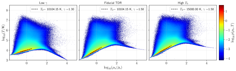
Figure 2: Joint, volume-weighted distribution of the temperature and density of baryons in our simulation at $z=2.2$. Center: the fiducial $(T_{0},\gamma)$ parameter case (values obtained by fitting a power-law through gas temperatures and densities). Left: the case with rescaled temperatures for a lower $\gamma$ than the fiducial and the same $T_{0}$. This can be seen to affect the slope of the TDR by a twisting of the 2D distribution. Right: the case with rescaled temperatures for a higher $T_{0}$ than the fiducial and the same $\gamma$. The entire distribution is shifted along the $\log_{10}(T/$K) axis, keeping the shape the same. (Note that the color-bar label is using shorthand for $p(\log_{10}(\rho_{\mathrm{b}}/\bar{\rho}_{\mathrm{b}}),\log_{10}(T/$K$))$.)

The baryon component in our simulation can be seen to follow a very tight temperature-density relation (TDR) that can be modelled by a power-law of the form (Hui & Gnedin, 1997)

$$T=T_{0}\bigg{(}\frac{\rho_{\text{b}}}{\bar{\rho}_{\text{b}}}\bigg{)}^{\gamma-1},$$ (1)

where $\bar{\rho}_{\text{b}}$ is the mean density of the gas, and $T_{0}$ (a temperature at the mean gas density) and $\gamma$ (adiabatic power-law index) are the two free parameters of this model. Indeed, a strong systematic $\rho_{\mathrm{b}}$-$T$ relationship is visually apparent in a slice through our simulation box (Figure 1). We perform a linear least-squares fit of the above relation through our simulation in the range $-0.5<\log_{10}(\rho_{\text{b}}/\bar{\rho}_{\text{b}})<0.5$ and $\log_{10}(T/\text{K})<4$. The best-fit (fiducial) values are $T_{0}=10104.15$ K and $\gamma=1.58$. While a range of works have demonstrated the potential of using different summary statistics of the Ly$\alpha$ forest as probes to measure $T_{0}$ and $\gamma$ (see e.g. Gaikwad et al., 2020), in this work we highlight a first field-level framework for inference of these two thermal parameters of the IGM.

The following strategy is adopted for sampling the parameter space of $(T_{0},\gamma)$ to produce labelled data for the supervised training of the inference machine. Both the parameters are varied by a small amount at a time, $\log T_{0}\to\log T_{0}+\log x$ and $\gamma\to\gamma+y$ to obtain a new TDR. We then rescale the simulated temperatures at every cell of the simulation by $T\to x\cdot(\rho_{\text{b}}/\bar{\rho}_{\text{b}})^{y}\cdot T$ at fixed densities $\rho_{\text{b}}$ to appropriately incorporate the scatter off the TDR into our mock data, effectively conserving the underlying $T$-$\rho_{\mathrm{b}}$ distribution rather than drawing from a pure power-law. This procedure is illustrated in Figure 2 with the help of the full 2D histograms of temperature and density for two individual parameter rescalings as well as the fiducial case.

2.2 Mock Lyman-$\alpha$ Forest

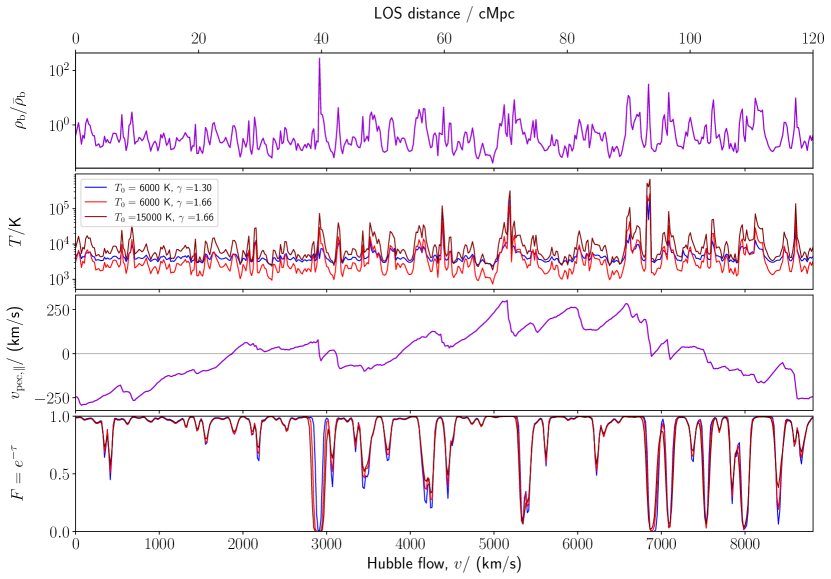
Figure 3: Simulated baryon overdensities, temperatures, line-of-sight peculiar velocity, and transmission along an example skewer through our box for three different temperature-density relations – one pair each for fixed $T_{0}$ and fixed $\gamma$ – to indicate characteristic variations w.r.t the two TDR parameters.The line shifts due to the peculiar velocity component ($v_{\text{pec},\parallel}$) can be easily noticed. Since the rescaling of the temperatures depends on the densities, inhomogeneous differences are seen in the skewer temperatures in the cases with varying $\gamma$. The absorption lines are broader where the temperatures are higher and the amount of broadening is also a function of densities being probed through $\gamma$.

In order to simulate the Ly$\alpha$ forest transmission $F=e^{-\tau}$ ($\tau$ being the optical depth), we first choose $10^{5}$ random lines of sight (a.k.a. skewers) parallel to one of the Cartesian sides (e.g. Z-axis) of the box by picking all consecutive 4096 voxels along that axis while keeping the other two coordinates (X and Y) fixed at a time. The Ly$\alpha$ optical depth at an output pixel in a spectrum is calculated from the information of the density, temperature, and the LOS component of gas peculiar velocity ($v_{\mathrm{pec},\parallel}$) at each corresponding voxel along the given skewer. Here, the gas is reasonably assumed to be in ionization equilibrium among the different species of H and He and further that He is almost completely (doubly) ionized at $z\sim 2.2$ (i.e. $x_{{He\textsc{iii}}}\approx 1$; Miralda-Escudé et al. 2000, Becker et al. 2015) in order to estimate the neutral H density, $n_{{H\textsc{i}}}$ for each of those voxels. The Ly$\alpha$ optical depth at a pixel with Hubble velocity $v$ and gas peculiar velocity $v_{\mathrm{pec},\parallel}$ is estimated as

$$\tau(v)=\frac{\pi e^{2}\lambda_{\mathrm{Ly}\alpha}f_{lu}}{m_{\mathrm{e}}cH(z)}\int n_{{H\textsc{i}}}(v^{\prime})\phi_{\mathrm{D}}\big{(}v^{\prime};v+v_{\mathrm{pec},\parallel},b\big{)}dv^{\prime},$$ (2)

where the rest-frame $\lambda_{\mathrm{Ly}\alpha}=1215.67$ Å, the Ly$\alpha$ oscillator strength $f_{lu}=0.416$, and

$$\phi_{\mathrm{D}}(v;v_{0},b)\equiv\frac{1}{b\sqrt{\pi}}\exp\Bigg{[}-\bigg{(}\frac{v-v_{0}}{b}\bigg{)}^{2}\Bigg{]}$$ (3)

is the Doppler line profile with the temperature-dependent broadening parameter $b=\sqrt{2k_{\mathrm{B}}T/m_{\mathrm{H}}}$. These $\tau$ values are additionally rescaled by a constant factor such that the mean Ly$\alpha$ transmission in our full set of $10^{5}$ skewers matches its observed value of $\bar{F}_{\mathrm{obs}}=0.86$, compatible with Becker et al. (2013).

To mimic observational limitations and minimize the impact of numerical noise in the simulations, we restrict the Fourier modes within the spectra to $k<k^{*}$, $k^{*}=0.18$ s km^-1. This is effectively achieved by smoothing them with a spectral resolution kernel of $R_{\mathrm{FWHM}}\approx 60,000$ and additionally rebinning them by 8-pixel averages, matching the Nyquist sampling limit. The final size of a spectrum in our analysis is thus 512 pixels.

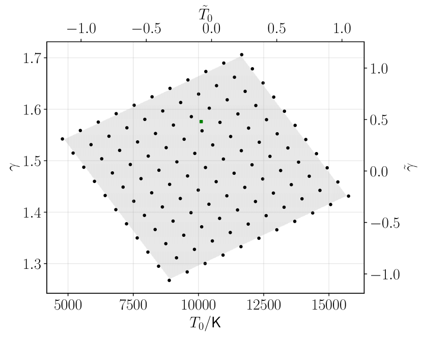
Figure 4: Our sample of thermal models for the various training and test purposes that contains 11$\times$11 (121) distinct $(T_{0},\gamma)$ combinations. The fiducial TDR parameter combination is depicted as the green square. The rescaled $(\tilde{T}_{0},\tilde{\gamma})$ axes are also shown for context (see Section 3.1). This is a uniform grid in a parametrization that captures the well known degeneracy direction in the $(T_{0},\gamma)$ space. The grey-shaded area shows our prior range in this parameter space. Please refer to Appendix A for more details regarding the strategy used for this sampling.

When sampling the $(T_{0},\gamma)$ space, new mock spectra are produced for each parameter combination with the new (rescaled) temperatures and the original densities and line-of-sight peculiar velocities along the same set of skewers.

An example skewer is shown in Figure 3 for three different TDRs. Since the temperature rescaling is a function of $\rho_{\text{b}}/\bar{\rho}_{\text{b}}$ through $\gamma$, characteristic differences in skewer temperatures and Ly$\alpha$ transmission between cases with varying $\gamma$ are visible. In this work, we sample a grid of 11$\times 11$ $(T_{0},\gamma$) combinations as shown in Figure 4 – for each of which we have the same set of $10^{5}$ skewers – for training and testing our deep learning machinery. This grid is oriented in a coordinate system that captures the well-known degeneracy direction in the $(T_{0},\gamma)$ space as identified in many TPS analyses (e.g. Walther et al. 2019) and is motivated by the heuristic argument that it is easiest to train a neural network for inference with an underlying parametrization that captures the most characteristic variations in the data. The exact sampling strategy is further described in Appendix A. We use the grey-shaded region in that figure as our prior range of parameters having a uniform prior distribution in all our further analyses.

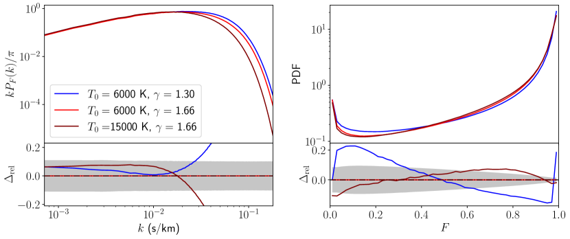
Figure 5: Transmission power spectrum (left) and transmitted PDF (right) computed from our set of $10^{5}$ skewers for three TDR parameter combinations, the same as in Figure 3. The fractional differences between different TDR cases are shown in the corresponding bottom panels with the grey-shaded areas as $1\sigma$ uncertainty ranges (bands drawn from discrete $k$-modes in TPS and discrete histogram bins in TPDF), equivalent of 100 spectra.

2.3 Summary Statistics

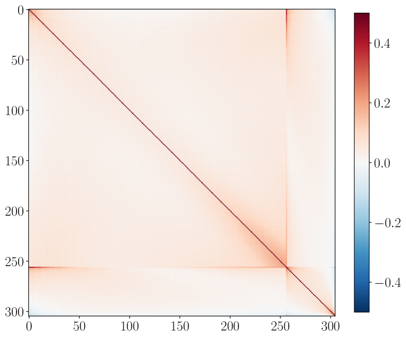
Figure 6: Correlation matrix of the joint summary vector (the first 256 entries being TPS and the later 49 being TPDF) estimated from our set of $10^{5}$ mock spectra for the fiducial thermal model. Notice the mild correlations within the individual summaries and the cross-correlations between the two summaries.

We consider two summary statistics – TPS and TPDF – of the Ly$\alpha$ forest in this work for demonstrating the benefit of field-level inference. The TPS is defined here as the variance of the transmitted “flux contrast” $\delta_{F}\equiv(F-\bar{F})/\bar{F}$ in Fourier space, i.e., $P_{F}(k)\sim\langle\tilde{\delta}(k)^{*}\cdot\tilde{\delta}(k)\rangle$. For a consistent comparison of inference outcomes, we apply the same restriction $k<0.18$ s km^-1 as in the input to our deep learning machinery (see Section 2.2). To obtain the TPDF, we consider the histogram of the transmitted flux $F$ in the full set of skewers over 50 bins of equal width between 0 and 1. For the likelihood analysis with the TPDF we leave the last bin out as it is fully degenerate with the rest due to the normalization of the PDF. The mean TPS and TPDF computed from the $10^{5}$ skewers for three different TDR parameter combinations are shown in Figure 5 along with the relative differences in both the statistics between pairs of TDR models. The uncertainty range shown as a grey band therein corresponds to $1\sigma$ equivalent of 100 spectra. We also compute the joint covariance matrix of the concatenated summary vector of TPS and TPDF from our full set of mock spectra by the estimator

$$\mathbf{C_{s}}=\frac{1}{N-1}\sum_{i=1}^{N}(\mathbf{s}_{i}-\mathbf{\bar{s}})^{T}(\mathbf{s}_{i}-\mathbf{\bar{s}}),$$ (4)

where $N=10^{5}$ and $\mathbf{s}$ is a vector of which the first 256 entries are the Fourier modes in the TPS ($k<k^{*}$) and the later 49 entries are the bins in the TPDF, $F\in[0,1)$. The joint correlation matrix for a thermal model from our sample is shown in Figure 6. Mild correlations among relatively close entries within the TPS or the TPDF can be observed as well as moderate cross-correlations between the two summary statistics.

For inference with these summary statistics, we cubic-spline interpolate both (the TPDF per histogram bin and the TPS per discrete $k$-mode) as a function of the parameters $(T_{0},\gamma)$ to obtain an emulator over our prior range as depicted in Figure 4 where we assume a flat (uniform) prior in both the parameters. We verified that choosing a different interpolation scheme, e.g. linear, does not strongly affect the results of the inference.

3 Field-level Inference Machinery

As described in Section 2, we have simulated Ly$\alpha$ forest absorption profiles (spectra) from hydrodynamic simulations having known thermal $(T_{0},\gamma)$ parameter values. The aim of our machinery is to learn the characteristic variations in the spectra (i.e., at field-level) w.r.t. those parameters in order first to distinguish between two adjacent thermal models and ultimately also to provide an uncertainty estimate as well as a point estimate of the parameter values whereby Bayesian inference can be performed. Thus framed, this is a very well-suited problem for application of supervised machine learning. The output of a fully-trained deep neural network can be used as a model (emulator) for a newly-learned, optimal “summary statistic” of the Ly$\alpha$ transmission field that is fully degenerate with the thermal parameters, hence carrying most of the relevant information about them that the full field offers.

In the following we describe our framework in detail, with special focus on the neural network architecture and training.

3.1 Overview

The general structure of inference with Ly$\alpha$NNA entails a feed-forward 1D ResNet neural network called “Sansa” that connects an underlying input information vector (transmission field) to an output “summary vector” that can be conveniently mapped to the thermal parameters $(T_{0},\gamma)$. Ideally, we expect this summary vector to be a direct actual estimate of the parameters itself, however, due to a limited prior range of thermal models available for training, a systematic (quantifiable) bias is observed in the pure network estimates (see Appendix B). Nonetheless, these estimates can be mapped to the parameters via a tractable linear transformation. For brevity our network encompasses this mapping such that its output is a direct estimate of the parameters $\mathbf{\tilde{\pi}}=(\tilde{T}_{0}$, $\tilde{\gamma})$. As an estimate of its own uncertainty of a given prediction, the network also returns a parameter covariance matrix $\tilde{\mathbf{C}}$. Since our two parameters have dynamic ranges different by orders of magnitude, we linearly rescale them as $T_{0}\to\tilde{T}_{0}$ and $\gamma\to\tilde{\gamma}$, to fall in the same range $\sim(-1,1)$. This bijective mapping ensures numerical stability of the point estimates by the networks and is a common practice for deep learning regression schemes. The output covariance matrix (and its inverse) must be positive-definite as a mathematical requirement. This is ensured in our framework in a way similar to Fluri et al. (2019) by a Cholesky decomposition of the form

$$\tilde{\mathbf{C}}\mathbf{{}^{-1}}=\mathbf{L}{\mathbf{L}}^{T},$$ (5)

where $\mathbf{L}$ is a lower triangular matrix. Our network predicts the three independent components of that matrix ($\log{L_{11}}$, $\log{L_{22}}$, $L_{12}$ to further ensure uniqueness) rather than the covariance matrix directly. The network is optimized following a Gaussian negative log-likelihood loss (hereinafter NL3),

$$\mathcal{L}(\tilde{\pi})=\log|\tilde{\mathbf{C}}|+(\tilde{\pi}-\hat{\pi})\tilde{\mathbf{C}}\mathbf{{}^{-1}}(\tilde{\pi}-\hat{\pi})^{T},$$ (6)

where $\hat{\pi}=(\hat{T}_{0},\hat{\gamma})$ are the true parameter labels. This can be seen as an extension of the conventional mean-squared error, MSE $=(\tilde{\pi}-\hat{\pi})(\tilde{\pi}-\hat{\pi})^{T}$, in the presence of a network-estimated covariance. It can be noted that the covariance matrix does not have any labels and is primarily a way to regularize network predictions under a Gaussian likelihood assumption.

3.2 Architecture

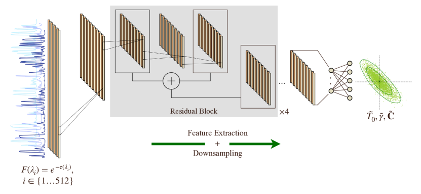
Figure 7: A schematic representation of the architecture of Sansa. It comprises a 1D residual convolutional neural network with four residual blocks in series for extracting crucial features from the spectra of size 512 pixels, followed by a fully-connected layer to map the outcome to the parameter point predictions $\mathbf{\tilde{\pi}}$ and a covariance estimate $\mathbf{\tilde{C}}$ over 5 output neurons.

We build our architecture using the open-source Python package TensorFlow/Keras (Chollet et al., 2015). The neural network for field-level inference with Ly$\alpha$NNA is called Sansa and consists of a 1D ResNet (He et al., 2015a), a residual convolutional neural network that extracts useful features from spectra and turns them into a “summary” vector which can then be used for inference of model parameters. Figure 7 shows a schematic representation of the architecture of Sansa. The input layer consists of 512 spectral units. This input is passed through four residual blocks in series with varying numbers of input/output units, each block having the same computational structure as illustrated in Figure 8. Each residual block is followed by a batch-normalization and an average-pooling layer to downsample the data vectors consecutively. A ResNet architecture is particularly attractive because of its ease of convergence during training owing to predominantly learning the residual mappings that could conveniently be driven to zero if identity maps are the most optimal in intermediate layers. This is achieved by introducing “skip-connections” in a sequential convolutional architecture that fulfil the role of identity (linear) functions. The residual blocks can more easily adapt to those linear mappings than having to train non-linear layers to mimic them. A special advantage of the skip-connections is that they do not introduce more parameters than a sequential counterpart. Our neural network has a total of 136,784 trainable parameters that are tuned via back-propagation. We use the TensorFlow in-built leaky ReLU (rectified linear unit) function for all the non-linear activations in the residual blocks with the negative-slope of 0.3. The resultant set of feature-tensors is flattened into a single vector of size 128 and mapped to the output vector $(\tilde{T}_{0},\tilde{\gamma},\log L_{11},\log L_{22},L_{12})$ with a fully-connected, unbiased linear layer. We regularize the network kernels with a very small L2 weight decay ($\mathcal{O}(10^{-7})$ in the convolutional layers, $\mathcal{O}(10^{-8})$ in the fully connected layer). We also use a dropout (Srivastava et al., 2014) of 0.14 after each residual block during training for encouraging generalization.

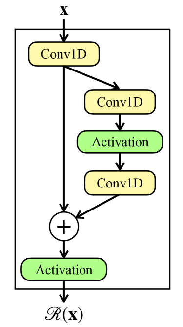
Figure 8: A residual block in Sansa. An input vector $\mathbf{x}$ is first passed through a convolutional layer and a copy of the output tensor is made which consecutively goes through a pair of convolutional layers introducing nonlinearity, all the while preserving the shape of the output tensor. The outcome is then algebraically added to the earlier copy (i.e. a parallel, identity function) and the sum is passed through a nonlinear activation to obtain the final outcome of the block. The latter two convolutional layers thus learn a residual nonlinear mapping.

3.3 Training

All convolutional kernels in Sansa are initialized following the approach of Glorot & Bengio (2010) and the weights in the final linear layers are initialized similarly to He et al. (2015b). After a preliminary convergence test w.r.t. training data-set size, we chose a training set consisting of 24,000 spectra from each thermal model in our sample. Moreover, we have a separate validation set for monitoring overfitting viz. 1/3 the size of the training set with an equivalent distribution of spectra among thermal models. The network is trained by minimizing the NL3 loss function in Eq. (6). Additionally, three other metrics are monitored during the training: $\log|\tilde{\mathbf{C}}|$, $\chi^{2}=(\tilde{\pi}-\hat{\pi})\tilde{\mathbf{C}}\mathbf{{}^{-1}}(\tilde{\pi}-\hat{\pi})^{T}$, and the MSE. Notice that the loss function is simply the sum of the first two metrics.

The training is performed by repeatedly cycling through the designated training data-set in randomly chosen batches of a fixed size. Each cycle through the data is deemed an “epoch”, and each back-propagation action on a batch is termed a “step of training”.

We expect the $\chi^{2}$ metric to optimally take the value $\sim N_{\mathrm{par}}$ because of the underlying Gaussian assumption (in our case $N_{\mathrm{par}}=2$). The improvement of the network during training is then in large parts due to a decrement in $\log|\tilde{\mathbf{C}}|$ which indicates that the network becomes less uncertain of its estimates as the training progresses. The state of a network is said to be improving if the value of NL3 decreases and the network $\chi^{2}$ remains close to 2 for data unseen during back-propagation, the validation set. Therefore, we deem the best state of the network to be occuring at the epoch during training at which the validation NL3 is minimal while the validation $|\chi^{2}-2|<\epsilon$, for a small $\epsilon=0.05$. We use the Adam optimizer (Kingma & Ba, 2014) with an initial learning-rate of $2\times 10^{-5}$ and a learning-rate schedule in the form of a stepwise exponential decay of 2.5$\%$ every ten epochs. The Adam moment parameters have the values $\beta_{1}=0.99$ and $\beta_{2}=0.999$. We performed a Bayesian hyperparameter tuning for fixing the values of kernel weight decays, the dropout rate, and the optimizer moment $\beta_{1}$ parameter. Please refer to Appendix C for a further description of our strategy for choosing optimal hyperparameters for our network architecture and training. We present the progress of the network’s training quantified by the four metrics mentioned above in Appendix D.

3.4 Ensemble Learning

The initialization of our network weights (kernels) as well as the training over batches and epochs is a stochastic process. This introduces a bias in the network predictions that can be traded for variance in a set of randomly initialized and trained networks. Essentially, if the errors in different networks’ predictions are uncorrelated, then combining the predictions of multiple such networks helps in improving the accuracy of the predictions. It has been shown that a “committee” of neural networks could outperform even the best-performing member network (Dietterich, 2000). This falls under the umbrella of “ensemble learning”.

Once we have an optimal set of hyperparameter values for Sansa, we train ten neural networks with the exact same architecture and the learning hyperparameters but initializing the network weights with different pseudo-random seeds and training with differently shuffled batches of the data-set. The output predictions by all the member networks of this committee of $N_{\textsc{Sansa}}=10$ neural networks are then combined in the form of a weighted averaging of the individual predictions to obtain the final outcome (this is commonly known as bootstrap aggregating or “bagging”; see e.g. Breiman 2004). For a given input spectrum $x$, let $\mathcal{S}_{i}(x)$ denote the output point predictions by the $i$th network in our committee. Then the combined prediction of the committee is

$$\mathcal{S}(x)=\frac{1}{N_{\textsc{Sansa}}}\sum_{i}\frac{1}{|\mathbf{\tilde{C}}_{i}(x)|}\mathcal{S}_{i}(x),$$ (7)

where $\mathbf{\tilde{C}}_{i}(x)$ is the output estimate of the covariance matrix by the $i$th network for the input spectrum $x$. This combination puts more weight on less uncertain network predictions and thus is optimally informed by the individual network uncertainties. Even with such a small number of cognate members, we observe slight improvements w.r.t. the best-performing member as discussed in Appendix E. All the output point predictions by Sansa considered in the following part of the text are implicitly assumed to be that of the committee and not of an individual network unless specified otherwise.

3.5 Inference

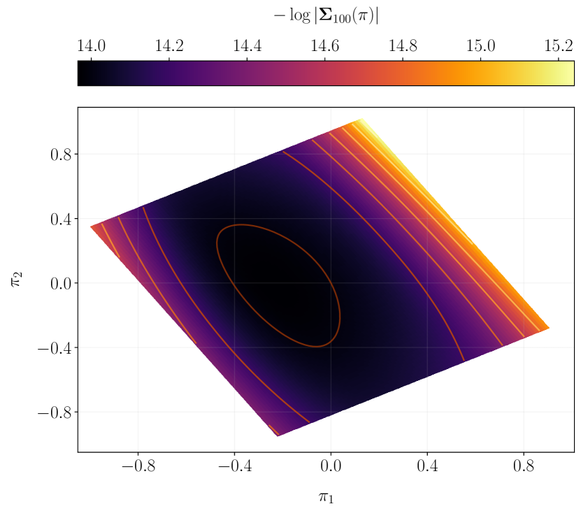
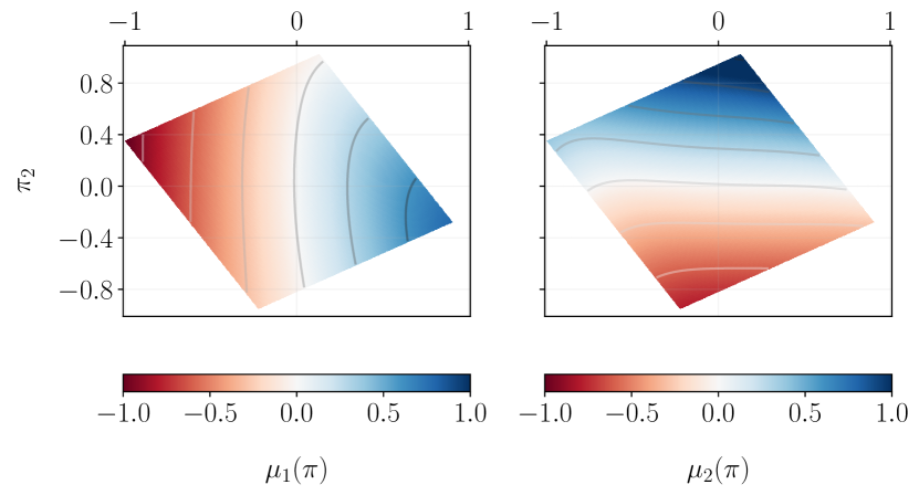
Figure 9: The likelihood model of inference with Sansa over our prior range for the rescaled $\pi$ parameters. The top panel shows a measure of the covariance model $\mathbf{\Sigma(\pi)}$ and the bottom panels the model for the two rescaled parameters, $\mu_{1}\equiv\tilde{T}_{0}$ and $\mu_{2}\equiv\tilde{\gamma}$. Notice the orientation of the covariance model in the degeneracy direction in the parameter space. The model for the mean fairly approximate $\mu_{i}(\pi)=\pi_{i}$ as expected.

We perform Bayesian inference of the model parameters with Sansa as well as the traditional summary statistics introduced in Section 2.3. In all the cases, we assume a Gaussian likelihood and a uniform prior over the range shown in Figure 4. For inference with Sansa we create an emulator for a likelihood analysis in the following way. A test set of spectra for a given truth $(\hat{T}_{0},\hat{\gamma})$ are fed into Sansa and a corresponding set of parameter point estimates $(\tilde{T}_{0},\tilde{\gamma})$ are obtained. Owing to our optimization strategy (described in Section 3.3) these network predictions have an inherent scatter that is consistent with a network covariance estimate $\mathbf{\tilde{C}}$. A mean point prediction $\bar{\pi}=(\bar{T}_{0},\bar{\gamma})$ and a covariance matrix is estimated from the scatter of the point estimates. This is performed for each of our 121 thermal models in the test sample. We then cubic-spline interpolate the mean network point prediction and the scatter covariance over our prior range of thermal parameters $\mathbf{\pi}$ to obtain a model (emulator)$\big{[}\mathbf{\mu(\pi)},\mathbf{\Sigma(\pi)}\big{]}$. The advantage of creating such a model for the likelihood is that the inference results of our machinery could, in principle, be combined with other probes of interest to further constrain our knowledge of the thermal state of IGM. This emulator is then used to perform an MCMC analysis for getting posterior constraints with a likelihood function,

$$\log L_{N}(\mathbf{\pi})\sim-\frac{1}{2}\Big{[}\log|\mathbf{\Sigma}_{N}(\pi)|-(\bar{\pi}_{N}-\mu(\pi))\mathbf{\Sigma}_{N}\mathbf{{}^{-1}(\pi)}(\bar{\pi}_{N}-\mu(\pi))^{T}\Big{]},$$ (8)

where $\bar{\pi}_{N}$ is the mean network point prediction for a given set of $N$ test spectra and $\mathbf{\Sigma}_{N}(\pi)=\mathbf{\Sigma}(\pi)/N$ quantifies the uncertainty in the mean point estimate for the given data-set size. We show this model in Figure 9. The degeneracy direction in the parameter space is retained as seen in the covariance model, $\mathbf{\Sigma}_{100}(\pi)$. The model for the mean parameter values, $\mu(\pi)$, consists of rather smoothly varying functions approximating $\mu_{1,2}(\pi_{1},\pi_{2})=\pi_{1,2}$, conforming to our expectation.

4 Results and Discussion

In this section, we show the results of doing mock inference with our machinery as described in Section 3 and compare them with a summary-based approach (see Section 2.3 for more details on the summaries used). We investigate a few different test scenarios for establishing robustness of our inference pipeline.

We consider a test set of spectra that are distinct from those used in training and validation to evaluate the performance of our inference pipeline for previously unseen data (note that we build the likelihood model for Sansa using the validation set). This set consists of 4,000 spectra for a given underlying true thermal model $(\hat{T}_{0},\hat{\gamma})$. In Figure 10, we show the output scatter of point estimates by Sansa for the fiducial TDR, $\hat{T}_{0}=10104.15$ K and $\hat{\gamma}=1.58$, with contours of 68% and 95% probability (note that this model is off the training grid, as shown in Figure 4). For comparison, we also plot the posterior contours (obtained by Sansa following the strategy outlined in Section 3.1), inflated to emulate the uncertainty equivalent of one input spectrum. A very good agreement is observed between both the cases, suggesting that a cubic-spline interpolation of the scatter covariance is a sufficiently good emulator for a likelihood analysis as discussed in Section 3.5.

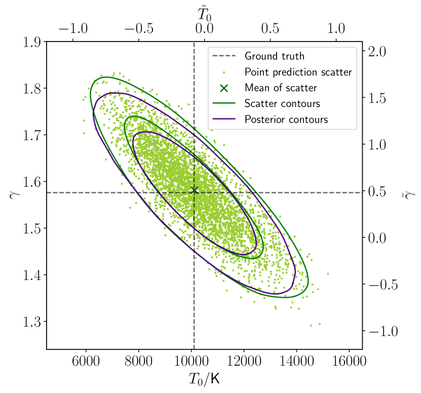
Figure 10: Scatter of point predictions for the test set of spectra from our fiducial TDR model shown here with the 68% and 95% contours (green). The contours of the posterior distribution (red) obtained by Sansa with the procedure outlined in Section 3.1, inflated to match the information equivalent of one spectrum, follow the scatter contours very closely. Sansa also recovers the true parameters (dashed) with a very good accuracy, as indicated by the mean of the point prediction scatter (green cross).

We perform additional tests to establish the robustness of the network performance under physically meaningless modifications of the spectra. These include rolling them along the spectral axis (allowed since the underlying skewers follow periodic boundary conditions) and flipping the direction of the spectral axis (i.e., a “mirror-spectrum”). These modification do not change the physical characteristics of the spectra dictated by the thermal state of the IGM and hence carry the same information of the TDR parameters. We perform inference with Sansa with the 4,000 test spectra from the fiducial thermal model while (i) rolling them by a quarter of a skewer (i.e., 128 pixels), labelled as “Rolled-q”, (ii) rolling them by a semi-skewer (i.e., 256 pixels), labelled as “Rolled-s”, and (iii) flipping them along the spectral axis, labelled as “Flipped”. Since Sansa has a convolutional architecture, we expect such mathematical modifications of the input spectra to affect the inference outcome marginally. The posterior contours for all three cases are compared with the unmodified case in Figure 11. Indeed, the shape and size of all the contours agree extremely well with each other and the ground truth remains within the 68% contours. A good metric for comparison of the posterior constraints among the different cases can be expressed as

Table 1: $\chi^{2}_{\mathbf{\Delta}}$ values for different test scenarios for Sansa

Test	$\chi^{2}_{\mathbf{\Delta}}$
Original	2.02
Rolled-q	2.30
Rolled-s	2.40
Flipped	2.38

$$\chi^{2}_{\mathbf{\Delta}}\equiv\langle\mathbf{\Delta C^{-1}}\mathbf{\Delta}^{T}\rangle,$$ (9)

where $\mathbf{\Delta}_{i}=(\pi_{i}-\hat{\pi})$ is a point in the posterior MCMC sample, $\mathbf{C}$ is a covariance matrix of $\pi$ estimated from the posterior sample and the average $\langle\rangle$ is taken over the entire sample. For the different test scenarios described above, we measured the $\chi^{2}_{\mathbf{\Delta}}$ values (Table 1). For the test with unmodified spectra, this value is the smallest of all, although in all the modified cases it is also very close to each other and not too divergent from $N_{\mathrm{par}}=2$. This indeed points toward the robustness of Sansa’s performance under such augmentations of the data-sets even though they are not used while training the pipeline.

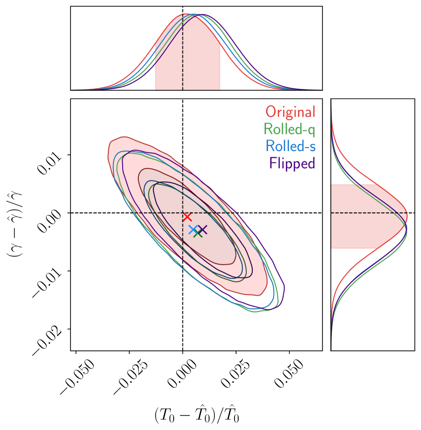
Figure 11: A comparison of posterior contours for different test scenarios with modified input spectra. “Rolled-q” and “rolled-s” denote the rollings of the spectral axis by 128 and 256 pixels, respectively. All of the contours carry an information equivalent of 100 skewers. A mean (expectation) value of all the posterior distributions are also shown with crosses of the corresponding colors. In all the cases, the ground truth falls within the 68% credibility contours.

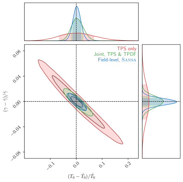
Figure 12: Posterior contours obtained by Sansa for the underlying fiducial thermal model. The posterior contours from the two traditional summary statistics are shown for comparison: (i) TPS only and (ii) joint constraints of TPS and TPDF where the cross-correlations of the summaries are accounted for by a joint covariance matrix. In terms of the size of the contours, the Sansa constraints are tighter than the TPS-only ones by a factor 5.65 and the joint constraints by 1.71, corroborating the claim that Sansa recovers relevant information for inference that is not carried by the TPS and/or the TPDF.

We compare the inference outcome of Sansa with the traditional summary statistics (TPS and TPDF) based procedure in terms of the area of the posterior contours ($\propto\sqrt{|\mathbf{C}|}$) as a figure of merit (FoM). We present the posterior constraints on $(\pi-\hat{\pi})/\hat{\pi}$ obtained by a MCMC analysis of TPS only, TPS and TPDF jointly, and Sansa for the fiducial thermal model in Figure 12. Evidently, the joint constraints of the two summary statistics are tighter than the TPS-only case as there is more information of the thermal parameter in the former. However, by far the field-level constraints by Sansa are tighter than both the traditional summary statistics cases, namely, a factor of 5.65 tighter compared to the TPS-only case and a factor of 1.71 tighter compared to the joint constraints in FoM. Indeed, the TPS is only a two-point statistic of the transmission field that has a highly non-Gaussian one-point PDF itself. Combining TPS and TPDF provides some more leverage, however, it still fails to account for some relevant parts of the information for inference. As illustrated by Figure 12, Sansa provides a remedy to the lost information by trying to optimally extract all the features of relevance at field-level.

5 Conclusion

We built a convolutional neural network architecture called Sansa for inference of the thermal parameters $(T_{0},\gamma)$ of the IGM with the Ly$\alpha$ forest at field-level. We trained this using a large set of mock spectra extracted from the nyx hydrodynamic simulations. For estimating posterior constraints, we created a reasonably robust pipeline that relies on the point predictions of the parameters and the uncertainty estimates by our neural network and that can in principle be easily combined with multiple other probes of the thermal state of the IGM. A comparison of our results with those of traditional summary statistics (TPS and TPDF in particular) revealed an improvement of posterior constraints in area of the credible regions by a factor 5.65 w.r.t. TPS-only and 1.71 w.r.t. a joint analysis of TPS and TPDF. Having a convolutional architecture, our neural network framework is mostly robust against physically meaningless modifications (e.g., rolling, flipping) of spectra, even though these are not applied to augment the data-set it is trained with.

However, our neural network that is trained with noiseless mock spectra for inference fails for spectra with even very small realistic noise (as small as CNR of 500 per 6 km/s). Indeed, our framework must be adapted for use with noisy spectra by retraining Sansa with data-sets containing artificially added noise that varies on-the-fly during training (to prevent learning from the noise).

Moreover, in the spirit of creating a robust pipeline for highly realistic spectral data-sets, a plethora of physical and observational systematic effects (such as limited spectral resolution, sky-lines, metal absorption lines, continuum fitting uncertainty, damped Ly$\alpha$ systems) must also be incorporated in the training data. This warrants a further careful investigation into training supervised deep learning inference algorithms with a variety of accurately modeled systematics added to our mock Ly$\alpha$ forest data-sets and we plan to carry it out in upcoming works.

Data Availability

The data/code pertaining to the analyses carried out in this paper shall be made publicly available.

Appendix A Orthogonal basis of the parameters

Heuristically, the training of the network is most efficient when our training sample captures the most characteristic variations in the data w.r.t. the two parameters of interest, $T_{0}$ and $\gamma$. Indeed, as found by many previous analyses (e.g., Walther et al. 2019), there appears to be an axis of degeneracy in the said parameter space given by the orientation of the elongated posterior contours. This presents us with an alternative parametrization of the space accessible via an orthogonalization of a parameter covariance matrix. By doing a mock likelihood analysis with a linear-interpolation emulator of the TPS on a pre-existing grid of thermal models, we first obtain a (rescaled) parameter covariance matrix $\mathbf{C}$ and then diagonalize that such that $\mathbf{\Lambda=V}^{T}\mathbf{CV}$ is a $2\times 2$ diagonal matrix ($\mathbf{V}$ symmetric). An “orthogonal” representation of the parameters can then be found by a change of basis,

$$\mathbf{A}^{T}=\mathbf{V\pi}^{T},$$ (10)

where $\mathbf{A}=(\alpha,\beta)$ and $\mathbf{\pi}=(T_{0},\gamma)$. In the above definition, $\beta$ represents the degeneracy direction in the $\pi$ parameters and $\alpha$ corresponds to the axis of the most characteristic deviation. Thence, we sample the parameter space for training with an 11$\times$11 regular grid in the orthogonal parameter space.

Appendix B Biases due to a limited prior range

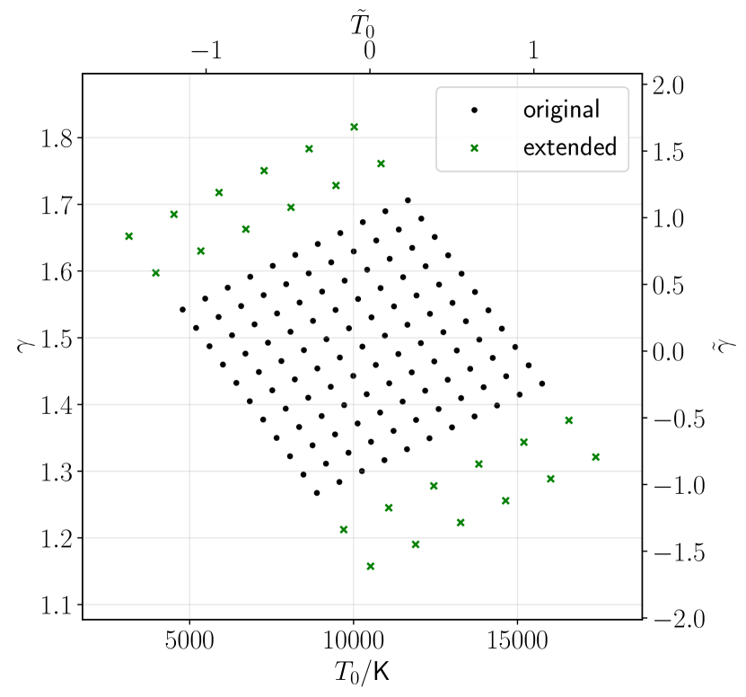
Figure 13: An extended grid of thermal models for regularizing the point predictions of Sansa. The extension is sparser than the actual training grid as it is only used for rectifying the skewed network predictions for models on the original grid by implicitly allowing a larger prior volume during training. No further test (or network validation) is performed for the models on the extended grid.

After a cursory network training we observed that when the true labels fall close to the edges of our prior range set by the training sample as shown in Figure 4, the mean network predictions are biased toward the center of that space. We also found that in the central region of our prior space, all the network predictions are roughly gaussian-distributed but closer to the edges of that prior they are more skewed, i.e., the mode of the distribution is closer to the ground truth than the median. To regularize this, we sampled an extended, sparser grid of thermal models along the degeneracy direction $\beta$ (in which Sansa provides weaker constraints), to augment our training data-set as shown in Figure 13. After retraining Sansa on this extended grid, we observed that a (quantifiable) bias still exists (Figure 14) but the predictions have mostly gaussianized. The mean point predictions for each of the thermal models on the original grid along a given orthogonal parameter axis fall on approximately a straight line, and hence we can perform a linear transformation of all the raw network predictions such that they satisfy our expectation, $\tilde{\pi}=\hat{\pi}$. This tractable transformation can be represented as follows. In the orthogonal parameters,

$$\mathbf{\tilde{A}}^{T}_{\text{f}}=\mathbf{M\tilde{A}}^{T}_{\text{i}}+\mathbf{c}^{T},$$ (11)

where $\mathbf{\tilde{A}}=(\tilde{\alpha},\tilde{\beta})$ is a point prediction vector in the orthogonal basis, $\mathbf{M}$ is a diagonal matrix and the subscripts “i” and “f” denote the original and transformed states of the vector respectively. This linear transformation is also shown for each parameter $\alpha$ and $\beta$ independently in Figure 14.

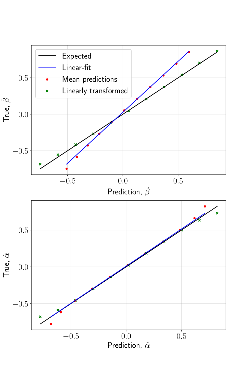
Figure 14: Mean point predictions on the validation set from a network trained on an extended grid as shown in Figure 13 and a straight line fit of each independent orthogonal parameter (averaged over the other). The mean predictions after applying the linear transformation can be seen to follow the expected $y=x$ behavior.

Note that since the change of basis is also a linear operation, the overall transformation in $\pi$ parameters is linear and preserves the gaussianity of the point predictions. Following Eq. (10), the transformation applied to the actual parameters $\tilde{\pi}$ looks like

$$\tilde{\pi}^{T}_{\mathrm{f}}=\mathbf{W}\tilde{\pi}^{T}_{\mathrm{i}}+\mathbf{d}^{T},$$ (12)

where $\mathbf{W=V^{-1}MV}$ and $\mathbf{d}=\mathbf{cV^{-1}}$ due to the symmetric $\mathbf{V}$. All the network covariance estimates $\mathbf{\tilde{C}}$ can also be linearly mapped with a matrix operation $\mathbf{\tilde{C}}\to\mathbf{W\tilde{C}W}^{T}$. We use our validation set to fit the linear transformation parameters, $\mathbf{W}$ and $\mathbf{d}$, for each trained neural network in the committee (the two parameter combinations (true labels) closest to the prior boundaries in each orthogonal parameter are not considered for this fitting). The full neural network Sansa presented in this paper has this tractable linear transformation incorporated as a final, unbiased layer.

Appendix C Hyperparameter optimization

As in every deep learning implementation, our algorithm is defined by a large set of hyperparameters that must be tuned in order to arrive at the best possible location on the bias-variance trade-off. Our hyperparameters include the dropout rate, the amplitude of the kernel regularization ($l_{2}$), number of residual blocks, number of filters and kernel-size in each residual block, weight-initialization, amount of downsampling per pooling layer, size of the batches of training data, Adam $\beta_{1}$ parameter, etc. Two strategies were adopted to explore this vast hyperparameter space. Hyperparameters having a finite number of discrete possible values (e.g. architecture in the residual parts) were manually tuned with informed heuristic choices of values to try. The size of the training batches is chosen in accordance with the learning rate such that the back-propagation steps are minimally stochastic and simultaneously exploratory of the weight-landscape. The rest of the hyperparameters having continuous spectra were tuned with a Bayesian optimization algorithm — based on a Gaussian process surrogate and an upper confidence bound (UCB) acquisition — for an optimal search of the space and an economical use of the resources. This was performed using the pre-defined routines of the python package Keras-Tuner (O’Malley et al. 2019).

Appendix D Training progress

We show the learning curves for Sansa in Figure 15 containing the four network metrics — MSE, $\chi^{2}$, $\log|\mathbf{\tilde{C}}|$ and the NL3 loss — for the best-performing network in our committee . Following our expectation, the values of the loss, MSE, and $\log|\mathbf{\tilde{C}}|$ decrease for the training and validation sets over the initial epochs and eventually the validation loss stops improving. On the other hand, $\chi^{2}$ for training converges to $\sim 2$ and that for validation fluctuates around the same value with a slow overall gain and a decrease in the amplitude of the fluctuations over the course of training. We restore the network to its state at an epoch $j^{*}$ at which the loss value is minimal while $|\chi^{2}-2|<0.05$ for the validation set. This helps us make sure that the network predictions are generalized enough and regularized under the Gaussian likelihood cost function. For this network $j^{*}=1140$. The same qualitative behavior is observed for all the networks in our committee.

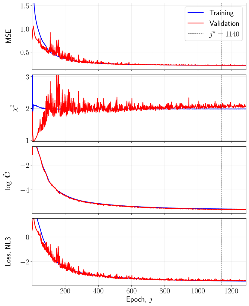
Figure 15: Learning curves of the best-performing network in the committee of Sansa. This network is trained for $\sim 1500$ epochs with a patience of 150 epochs for early-stopping. The best state of the network that can be possibly achieved is determined by the minimal value of NL3 while $|\chi^{2}-2|<0.05$ for the validation set and that occurs at epoch $j^{*}=1140$ during training.

Appendix E Single network vs. committee

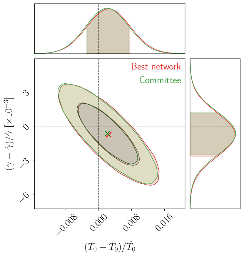
Figure 16: Comparison of the posterior contours obtain by the committee with those by the best-performing network in the committee for the fiducial thermal model with information equivalent of 1,000 spectra. The committee constraints are $\sim$6% tighter than those of the best member network.

As mentioned in Section 3.4, combining outputs of multiple similar neural networks is shown to improve the eventual outcome. Motivated by this, we employed a committee of ten networks with the same architecture but having different initial weights and training with different random batches. In practice, the likelihood model of inference described in Section 3.5 can be built for each individual network in the committee the same way as for the committee itself since the procedure relies purely on the predictions of the network(s) from the validation set. Hence, it is possible to compare the posterior constraints of an individual network with that of the committee. We present a comparison of the committee with the best-performing member network in Figure 16 and Table 2 for our test set of spectra from the fiducial thermal model. The constraints by the committee are 5.6% tighter than the best network in FoM and the value of $\chi^{2}_{\mathbf{\Delta}}$ is slightly smaller for the committee than for the best-performing network. Even though $N_{\textsc{Sansa}}=10$ is statistically a small number of sample members in a committee, the aggregate results of the ensemble are still somewhat better than the best-performing network, conforming to the popular findings.

Table 2: $\chi^{2}_{\mathbf{\Delta}}$ values for Sansa committee and the best-performing member

	$\chi^{2}_{\mathbf{\Delta}}$
Best network	2.26
Committee	2.19

References

- Almgren et al. (2013) Almgren, A. S., Bell, J. B., Lijewski, M. J., Lukić, Z., & Van Andel, E. 2013, ApJ, 765, 39
- Armengaud et al. (2017) Armengaud, E., Palanque-Delabrouille, N., Yèche, C., Marsh, D. J. E., & Baur, J. 2017, MNRAS, 471, 4606
- Becker et al. (2011) Becker, G. D., Bolton, J. S., Haehnelt, M. G., & Sargent, W. L. W. 2011, MNRAS, 410, 1096
- Becker et al. (2015) Becker, G. D., Bolton, J. S., Madau, P., et al. 2015, MNRAS, 447, 3402
- Becker et al. (2013) Becker, G. D., Hewett, P. C., Worseck, G., & Prochaska, J. X. 2013, MNRAS, 430, 2067
- Boera et al. (2019) Boera, E., Becker, G. D., Bolton, J. S., & Nasir, F. 2019, ApJ, 872, 101
- Boera et al. (2014) Boera, E., Murphy, M. T., Becker, G. D., & Bolton, J. S. 2014, MNRAS, 441, 1916
- Bolton et al. (2014) Bolton, J. S., Becker, G. D., Haehnelt, M. G., & Viel, M. 2014, MNRAS, 438, 2499
- Bolton et al. (2008) Bolton, J. S., Viel, M., Kim, T. S., Haehnelt, M. G., & Carswell, R. F. 2008, MNRAS, 386, 1131
- Boonkongkird et al. (2023) Boonkongkird, C., Lavaux, G., Peirani, S., et al. 2023, arXiv e-prints, arXiv:2303.17939
- Breiman (2004) Breiman, L. 2004, Machine Learning, 24, 123
- Busca & Balland (2018) Busca, N. & Balland, C. 2018, QuasarNET: Human-level spectral classification and redshifting with Deep Neural Networks
- Busca et al. (2013) Busca, N. G., Delubac, T., Rich, J., et al. 2013, A&A, 552, A96
- Chabanier et al. (2023) Chabanier, S., Emberson, J. D., Lukić, Z., et al. 2023, MNRAS, 518, 3754
- Chabanier et al. (2019) Chabanier, S., Palanque-Delabrouille, N., Yèche, C., et al. 2019, J. Cosmology Astropart. Phys., 2019, 017
- Chollet et al. (2015) Chollet, F. et al. 2015, Keras, https://keras.io
- Croft et al. (1998) Croft, R. A. C., Weinberg, D. H., Katz, N., & Hernquist, L. 1998, ApJ, 495, 44
- Cuceu et al. (2023) Cuceu, A., Font-Ribera, A., Nadathur, S., Joachimi, B., & Martini, P. 2023, Phys. Rev. Lett., 130, 191003
- Dawson et al. (2013) Dawson, K. S., Schlegel, D. J., Ahn, C. P., et al. 2013, AJ, 145, 10
- DESI Collaboration et al. (2022) DESI Collaboration, Abareshi, B., Aguilar, J., et al. 2022, AJ, 164, 207
- Dietterich (2000) Dietterich, T. G. 2000, in Multiple Classifier Systems (Berlin, Heidelberg: Springer Berlin Heidelberg), 1–15
- du Mas des Bourboux et al. (2020) du Mas des Bourboux, H., Rich, J., Font-Ribera, A., et al. 2020, ApJ, 901, 153
- Fluri et al. (2019) Fluri, J., Kacprzak, T., Lucchi, A., et al. 2019, Phys. Rev. D, 100, 063514
- Fluri et al. (2018) Fluri, J., Kacprzak, T., Refregier, A., et al. 2018, Phys. Rev. D, 98, 123518
- Gaikwad et al. (2020) Gaikwad, P., Rauch, M., Haehnelt, M. G., et al. 2020, MNRAS, 494, 5091
- Gaikwad et al. (2021) Gaikwad, P., Srianand, R., Haehnelt, M. G., & Choudhury, T. R. 2021, MNRAS, 506, 4389
- Garzilli et al. (2012) Garzilli, A., Bolton, J. S., Kim, T. S., Leach, S., & Viel, M. 2012, MNRAS, 424, 1723
- Glorot & Bengio (2010) Glorot, X. & Bengio, Y. 2010, in Proceedings of Machine Learning Research, Vol. 9, Proceedings of the Thirteenth International Conference on Artificial Intelligence and Statistics, ed. Y. W. Teh & M. Titterington (Chia Laguna Resort, Sardinia, Italy: PMLR), 249–256
- Gordon et al. (2023) Gordon, C., Cuceu, A., Chaves-Montero, J., et al. 2023, arXiv e-prints, arXiv:2308.10950
- Gunn & Peterson (1965) Gunn, J. E. & Peterson, B. A. 1965, ApJ, 142, 1633
- Gupta et al. (2018) Gupta, A., Matilla, J. M. Z., Hsu, D., & Haiman, Z. 2018, Phys. Rev. D, 97, 103515
- Harrington et al. (2022) Harrington, P., Mustafa, M., Dornfest, M., Horowitz, B., & Lukić, Z. 2022, ApJ, 929, 160
- He et al. (2015a) He, K., Zhang, X., Ren, S., & Sun, J. 2015a, arXiv e-prints, arXiv:1512.03385
- He et al. (2015b) He, K., Zhang, X., Ren, S., & Sun, J. 2015b, arXiv e-prints, arXiv:1502.01852
- Hiss et al. (2019) Hiss, H., Walther, M., Oñorbe, J., & Hennawi, J. F. 2019, ApJ, 876, 71
- Hu et al. (2022) Hu, T., Khaire, V., Hennawi, J. F., et al. 2022, MNRAS, 515, 2188
- Huang et al. (2021) Huang, L., Croft, R. A. C., & Arora, H. 2021, MNRAS, 506, 5212
- Hui & Gnedin (1997) Hui, L. & Gnedin, N. Y. 1997, MNRAS, 292, 27
- Iršič et al. (2017) Iršič, V., Viel, M., Haehnelt, M. G., Bolton, J. S., & Becker, G. D. 2017, Phys. Rev. Lett., 119, 031302
- Jacobus et al. (2023) Jacobus, C., Harrington, P., & Lukić, Z. 2023, arXiv e-prints, arXiv:2308.02637
- Kacprzak & Fluri (2022) Kacprzak, T. & Fluri, J. 2022, Phys. Rev. X, 12, 031029
- Karaçaylı et al. (2023) Karaçaylı, N. G., Martini, P., Guy, J., et al. 2023, arXiv e-prints, arXiv:2306.06316
- Kingma & Ba (2014) Kingma, D. P. & Ba, J. 2014, arXiv e-prints, arXiv:1412.6980
- Lee et al. (2015) Lee, K.-G., Hennawi, J. F., Spergel, D. N., et al. 2015, ApJ, 799, 196
- Liang et al. (2023) Liang, Y., Melchior, P., Lu, S., Goulding, A., & Ward, C. 2023, arXiv e-prints, arXiv:2302.02496
- Lidz et al. (2010) Lidz, A., Faucher-Giguère, C.-A., Dall’Aglio, A., et al. 2010, ApJ, 718, 199
- Lukić et al. (2015) Lukić, Z., Stark, C. W., Nugent, P., et al. 2015, MNRAS, 446, 3697
- Lynds (1971) Lynds, R. 1971, ApJ, 164, L73
- McDonald et al. (2000) McDonald, P., Miralda-Escudé, J., Rauch, M., et al. 2000, ApJ, 543, 1
- McGreer et al. (2015) McGreer, I. D., Mesinger, A., & D’Odorico, V. 2015, MNRAS, 447, 499
- Meiksin (2000) Meiksin, A. 2000, MNRAS, 314, 566
- Melchior et al. (2022) Melchior, P., Liang, Y., Hahn, C., & Goulding, A. 2022, arXiv e-prints, arXiv:2211.07890
- Miralda-Escudé et al. (2000) Miralda-Escudé, J., Haehnelt, M., & Rees, M. J. 2000, ApJ, 530, 1
- Moriwaki et al. (2023) Moriwaki, K., Nishimichi, T., & Yoshida, N. 2023, Reports on Progress in Physics, 86, 076901
- Oñorbe et al. (2017) Oñorbe, J., Hennawi, J. F., Lukić, Z., & Walther, M. 2017, ApJ, 847, 63
- O’Malley et al. (2019) O’Malley, T., Bursztein, E., Long, J., et al. 2019, KerasTuner, https://github.com/keras-team/keras-tuner
- Palanque-Delabrouille et al. (2015) Palanque-Delabrouille, N., Yèche, C., Baur, J., et al. 2015, J. Cosmology Astropart. Phys., 2015, 011
- Palanque-Delabrouille et al. (2020) Palanque-Delabrouille, N., Yèche, C., Schöneberg, N., et al. 2020, J. Cosmology Astropart. Phys., 2020, 038
- Parks et al. (2018) Parks, D., Prochaska, J. X., Dong, S., & Cai, Z. 2018, Monthly Notices of the Royal Astronomical Society, 476, 1151
- Planck Collaboration et al. (2020) Planck Collaboration, Aghanim, N., Akrami, Y., et al. 2020, A&A, 641, A6
- Ravoux et al. (2023) Ravoux, C., Karim, M. L. A., Armengaud, E., et al. 2023, arXiv e-prints, arXiv:2306.06311
- Ribli et al. (2019) Ribli, D., Pataki, B. Á., Zorrilla Matilla, J. M., et al. 2019, MNRAS, 490, 1843
- Rogers & Peiris (2021) Rogers, K. K. & Peiris, H. V. 2021, Phys. Rev. Lett., 126, 071302
- Schaye et al. (2000) Schaye, J., Theuns, T., Rauch, M., Efstathiou, G., & Sargent, W. L. W. 2000, MNRAS, 318, 817
- Seljak et al. (2006) Seljak, U., Slosar, A., & McDonald, P. 2006, J. Cosmology Astropart. Phys., 2006, 014
- Slosar et al. (2013) Slosar, A., Iršič, V., Kirkby, D., et al. 2013, J. Cosmology Astropart. Phys., 2013, 026
- Srivastava et al. (2014) Srivastava, N., Hinton, G., Krizhevsky, A., Sutskever, I., & Salakhutdinov, R. 2014, J. Mach. Learn. Res., 15, 1929–1958
- Telikova et al. (2019) Telikova, K. N., Shternin, P. S., & Balashev, S. A. 2019, ApJ, 887, 205
- Theuns & Zaroubi (2000) Theuns, T. & Zaroubi, S. 2000, MNRAS, 317, 989
- Ďurovčíková et al. (2020) Ďurovčíková, D., Katz, H., Bosman, S. E. I., et al. 2020, MNRAS, 493, 4256
- Viel et al. (2013) Viel, M., Becker, G. D., Bolton, J. S., & Haehnelt, M. G. 2013, Phys. Rev. D, 88, 043502
- Viel et al. (2009) Viel, M., Bolton, J. S., & Haehnelt, M. G. 2009, MNRAS, 399, L39
- Viel et al. (2005) Viel, M., Lesgourgues, J., Haehnelt, M. G., Matarrese, S., & Riotto, A. 2005, Phys. Rev. D, 71, 063534
- Walther et al. (2021) Walther, M., Armengaud, E., Ravoux, C., et al. 2021, J. Cosmology Astropart. Phys., 2021, 059
- Walther et al. (2019) Walther, M., Oñorbe, J., Hennawi, J. F., & Lukić, Z. 2019, ApJ, 872, 13
- Wang et al. (2022) Wang, R., Croft, R. A. C., & Shaw, P. 2022, MNRAS, 515, 1568
- Wolfson et al. (2021) Wolfson, M., Hennawi, J. F., Davies, F. B., et al. 2021, MNRAS, 508, 5493
- Yèche et al. (2017) Yèche, C., Palanque-Delabrouille, N., Baur, J., & du Mas des Bourboux, H. 2017, J. Cosmology Astropart. Phys., 2017, 047
- Zaldarriaga (2002) Zaldarriaga, M. 2002, ApJ, 564, 153