Detecting Axion Dark Matter with Black Hole Polarimetry

Abstract

The axion, as a leading dark matter candidate, is the target of many on-going and proposed experimental searches based on its coupling to photons. Ultralight axions that couple to photons can also cause polarization rotation of light which can be probed by cosmic microwave background. In this work, we show that a large axion field is inevitably developed around black holes due to the Bose-Einstein condensation of axions, enhancing the induced birefringence effects. Therefore, we propose measuring the modulation of supermassive black hole imaging polarization angles as a new probe to the axion-photon coupling of axion dark matter. The oscillating axion field around black holes induces polarization rotation on the black hole image, which is detectable and distinguishable from astrophysical effects on the polarization angle, as it exhibits distinctive temporal variability and frequency invariability. We present the range of axion-photon couplings within the axion mass range $10^{-21}\text{--}10^{-16}\,\text{eV}$ that can be probed by the Event Horizon Telescope. The axion parameter space probed by black hole polarimetry will expand with the improvement in sensitivity on the polarization measurement and more black hole polarimetry targets with determined black hole masses.

I Introduction

Figure 1: The schematic diagram of the polarimetry of supermassive black holes (SMBH) with the axion star surrounding it. In this diagram, the small black circle denotes the SMBH, the large cyan circular cloud denotes the axion star in SMBH’s gravitational background, and $R_{*}$ denotes the radius of the axion star. When the light produced near the vicinity of the SMBH (orange dotted line) propagates through the axion star to the earth, the light’s polarization angle (blue solid arrowed lines) is rotated by the oscillating axion field with a rotation angle $\Delta\phi_{\text{polar}}$. Such variation on the polarization also has the time modulation with an angular frequency $\omega_{a}\sim m_{a}$, and the modulation is coherent over the size of the axion star.

The axion, proposed to solve a fundamental puzzle in strong interactions, is also a viable dark matter candidate [1, 2, 3, 4, 5, 6, 7, 8]. The current spectrum of axion expands to models that do not solve the puzzle, which motivates us to consider a broader range of axion parameters [9]. Laboratory searches for axions in the ultralight mass ranges ($m_{a}\lesssim 10^{-11}\,\text{eV}$) have also been proposed and performed. These experimental methods include magnetometers [10, 11, 12, 13, 14, 15, 16], cavities [17, 18, 19, 20, 21, 22, 23, 24, 25, 26, 27, 28, 29], and optical interferometers [30, 31, 32, 33]. On the other hand, astrophysical and cosmological observations placed the strongest bound on axion parameters in this mass range, such as the spinning down of black holes from superradiance [34, 35, 36], recurrent axinovae [37], spectral distortion [38, 39, 40, 41, 42], X-ray observations [43, 44, 45, 46, 47, 48, 49, 50], Gamma-ray observations [51, 52, 53, 54, 55, 56, 57], solar basin [58, 59], heating of dwarf galaxies [60, 61, 62], cosmic axion background [63, 64, 65], finite density effects inside stellars [66, 67], radio telescope [68, 69, 70, 71], and solar telescope [72, 73, 74]. In this work, we propose a complementary search on axions using the measurements on the modulation of electric vector position angle (EVPA) of black hole images. The polarization angle in the vicinity of black holes will experience birefringence effects from the dense axion field, which is developed through axion dark matter accretion onto black holes.

The axion field with masses $\lesssim 10^{-18}\,\text{eV}$, if accounts for the dark matter density, can rotate the polarization of light passing through it, which is known as the cosmic birefringence effect. It can be probed in cosmic microwave background (CMB) polarization measurements [75, 76, 77]. Extensive searches for axionlike polarizations in CMB have been recently performed by BICEP/Keck [78], POLARBEAR [79], and SPT-3G [80]. Other polarimetric observations can detect axion strings or axion dark matter are studied in Ref. [81, 82, 83, 84, 85, 86, 87, 88, 89, 90]. In our proposal, the axion field value is greatly enhanced compared to its expectation value predicted by the cosmic dark matter density due to the formation of axion stars in the gravitational potential well of black holes, increasing our sensitivity to axion-photon couplings. The first image of supermassive black holes (SMBH) M87^∗ by Event Horizon Telescope [91] opens the window into the new physics beyond the standard model that is only accessible around the Schwarzschild radius of black holes. Our axion stars near the supermassive black holes mostly have a size much larger than the Schwarzschild radius, therefore it does not necessarily require such high spatial resolution. The polarimetric studies of Event Horizon Telescope Targets have been performed actively with interferometric observations [92], further enabling us to use black hole polarimetry to study the birefringence effects induced by axion stars with larger radii.

Therefore, the crucial question becomes if the axion star formation rate is large enough to build up a large axion field value around the SMBH. Assuming axion is the dark matter, the self-scattering of ultralight axions is greatly enhanced due to the large phase density. Both numerical and analytical studies confirmed the formation of axion stars (sometimes called solitons) in dense dark matter halos from the gravitational scattering of axion waves or from the quartic self-couplings [93, 94, 95, 96, 97, 98, 99, 100], which provide us the tools to study the axion field value after the axion star formed. In current studies of axion stars, stable configurations of axion fields are numerically solved, with the dilute branch of axion stars being balanced by their gravity and kinetic pressure, while the dense branch is unstable due to the emission of relativistic axions [101, 102, 103]. In this work, we obtain a solution of stable axion field configurations in the black hole background, which allows a much larger stabilized axion field than the usual dilute branch. Stable axion stars around black holes will provide a significant and unique photon signal with a modulating polarization angle. Similar ideas were proposed in the context of axion cloud generated by black hole superradiance [104, 105, 106]. In our proposal, a broader axion mass range is probed with individual black holes since we do not rely on the axion cloud generated by superradiance. Our work demonstrates the great potential of using black hole polarimetry as detectors of axion dark matter, which will motivate both observational efforts on supermassive black holes and theoretical progress on the exact axion star formation rate in the black hole background.

II Axion Stars around black holes

In the following, we will study the solution of axion stars around black holes and the formation rate of such objects in the limit that the black hole is dominating the gravitational interaction, which will enable us to calculate the axion field value. Solving axion electrodynamics in the presence of axion fields, one would obtain modified Maxwell’s equations under which photons with different polarizations will propagate differently. The polarization angle shift induced by the axion field is [75, 76]

$$\Delta\phi_{\rm polar}=\frac{g_{a\gamma\gamma}}{2}[a_{\rm source}-a_{\rm earth}],$$ (1)

where $a_{\rm source}$ and $a_{\rm earth}$ are the axion field values at source and earth respectively. They are related to the energy density of axions $\rho_{a}$ and the axion mass $m_{a}$

$$a=\sqrt{2\rho_{a}/m_{a}^{2}}{\rm cos}(m_{a}t).$$ (2)

Therefore, if there is a significant difference in the axion amplitude between the source and the earth, the polarization angle shift can be large. It is crucial to calculate the axion field value developed around black holes to determine the exact value of the polarization angle induced by axions. We will study a new solution of stable axion stars around black holes and the formation rate of those axion stars to determine the axion field value.

II.1 Stable Axion Field Configuration Around Black Holes

The axion Lagrangian we consider in this work is

$$\begin{aligned} \mathcal{L}=-\frac{1}{4}F^{2}+\frac{1}{4}g_{a\gamma\gamma}aF\widetilde{F}+\frac{1}{2}\partial_{\mu}a\partial^{\mu}a-V(a),\end{aligned}$$ (3)

where the axion potential can be expressed as the quartic self-coupling and the mass term

$$\begin{aligned} V(a)\simeq\frac{1}{2}m_{a}^{2}a^{2}-\frac{\lambda}{4!}a^{4}.\end{aligned}$$ (4)

The quartic coupling can be related to the axion decay constant as $\lambda=m_{a}^{2}/f_{a}^{2}$. Axion-photon couplings can be parametrized as $g_{a\gamma\gamma}=c_{\gamma}\alpha_{\text{em}}/(2\pi f_{a})$ where $c_{\gamma}$ is a model-dependent constant. Although typically $c_{\gamma}\sim 1$, it could be enhanced in various models [107, 108]. We will treat $g_{a\gamma\gamma}$ as a free parameter and study the phenomenology of axion stars with axion-photon couplings.

We will study the axion star solution under the assumption $M_{\text{BH}}\gg M_{*}$, where $M_{*}$ is the axion star’s mass. For the moment we neglect the axion self-interactions arising from the axion potential, which will appear later when we calculate the critical mass of axion stars above which axion fields cannot remain stable. To describe axion’s profile in the background of the black hole quantitatively, we solve the Klein-Gordon equation

$$\begin{aligned} \nabla_{\mu}\nabla^{\mu}a=-V^{\prime}(a)\end{aligned}$$ (5)

in the black hole background, where $\nabla_{\mu}$ is the covariant derivative in the curved background of the black hole. To solve the time-dependent profile of axion, we write the axion profile as

$$\begin{aligned} a(r,t)=f_{a}\,\Theta(r)\cos(\omega_{a}t),\end{aligned}$$ (6)

where $\Theta(r)$ is the spatial-dependent part of the oscillation angle. The Schrodinger-Newton-type equation that governs the spatial part of the axion fields is written as

$$\boldsymbol{\nabla}^{2}\Theta=2\left(m^{2}_{a}\Phi+\frac{m^{2}_{a}-\omega^{2}_{a}}{2}\right)\Theta,$$ (7)

where

$$\begin{aligned} \Phi(r)\simeq-\frac{GM_{\text{BH}}}{r}\end{aligned}$$ (8)

is the gravitational potential of the black hole. Here, we have made the assumption $R_{*}\gg GM_{\rm BH}$, therefore the black hole can be approximated by a point-like source. Because we focus on the region where $M_{\text{BH}}\gg M_{*}$, we ignore the axion’s back reaction to the BH background. The contribution of the gravitational field of the BH has not been included in previous studies but is essential in this work to generate a significantly enhanced axion field in stable axion stars.

Noting that Eq. (7) has the same form as the Schrodinger equation for the electron radial wavefunction of the Hydrogen, we obtain the eigenfunction

$$\begin{aligned} \Theta(r)=\Theta_{0}\,e^{-GM_{\text{BH}}m_{a}^{2}r},\end{aligned}$$ (9)

and the eigenfrequency

$$\begin{aligned} \omega_{a}=m_{a}\sqrt{1-\left(GM_{\text{BH}}m_{a}\right)^{2}}.\end{aligned}$$ (10)

$\Theta(r)$ in Eq. (9) is the profile of the axion star in the ground state, which is spherically symmetric. $\omega_{a}$ in Eq. (10) is axion’s oscillation frequency given the ground state profile. The coefficient $\Theta_{0}$ represents $\Theta(r=0)$ and it needs to be determined by the amount of the mass accreted onto the gravitational potential well of black holes. A similar discussion on the ultralight particle in the gravitational background, referred to as the “gravitational atom”, can be found in [109, 110, 111]. From Eq. (9), we find that the axion star radius is

$$\begin{aligned} R_{*}\sim\frac{1}{GM_{\text{BH}}m_{a}^{2}},\end{aligned}$$ (11)

which is independent of the mass of the axion star. This is distinctly different from the mass-radius relation of self-gravitating axion stars which obeys $R_{*}^{\text{self}}\sim 1/(GM_{*}m_{a}^{2})$. Such difference can be explained by the difference in the gravitational energy of these two kinds of axion stars. For stable configurations, the gradient energy balances the gravitational energy, therefore the radii of these two axion stars have different $M_{*}$-dependence.

To estimate the axion star’s mass, we use the formula

$$\begin{aligned} M_{*}=\int d^{3}\boldsymbol{r}\,\rho_{*}\sim\rho_{*}R_{*}^{3},\end{aligned}$$ (12)

where $\rho_{*}$ is the energy density of axion star. We have

$$\begin{aligned} \rho_{*}\simeq\Big{\langle}\frac{1}{2}\dot{a}^{2}+\frac{1}{2}\nabla a^{2}+\frac{1}{2}m_{a}^{2}a^{2}-\frac{\lambda}{4!}a^{4}\Big{\rangle},\end{aligned}$$ (13)

where $\langle\cdots\rangle$ represents the time-averaged values, the first term is the oscillation energy, the second term is the gradient energy, the third term is the potential energy from axion’s mass term, and the fourth term is the potential energy from axion’s self-interaction. From Eq. (9), we find that the gradient energy is suppressed by an extra $(GM_{\text{BH}}m_{a})^{2}$ factor, therefore it is negligible when $GM_{\text{BH}}m_{a}\ll 1$. Before axion star’s mass reaches the critical value, the energy contribution from the self-interaction can also be neglected. Therefore, the axion star’s energy density can be approximately written as

$$\begin{aligned} \rho_{*}\sim m_{a}^{2}f_{a}^{2}\Theta_{0}^{2}.\end{aligned}$$ (14)

Substituting Eq. (11) and Eq. (14) into Eq. (12), we have

$$\begin{aligned} M_{*}\sim\frac{f_{a}^{2}\Theta_{0}^{2}}{G^{3}M_{\text{BH}}^{3}m_{a}^{4}},\end{aligned}$$ (15)

which reveals the relation between $M_{*}$ and $\Theta_{0}$. From Eq. (1), we have

$$\begin{aligned} \mathinner{\!\left\lvert\Delta\phi_{\text{polar}}\right\rvert}\simeq\frac{1}{2}g_{a\gamma\gamma}\Theta_{0}f_{a},\end{aligned}$$ (16)

where $\mathinner{\!\left\lvert\cdots\right\rvert}$ denotes the amplitude of oscillation. Combining Eq. (15) and Eq. (16), we can write the amplitude of polarization angle as

$$\begin{aligned} \mathinner{\!\left\lvert\Delta\phi_{\text{polar}}\right\rvert}\sim g_{a\gamma\gamma}\left(G^{3}M_{\text{BH}}^{3}m_{a}^{4}M_{*}\right)^{1/2},\end{aligned}$$ (17)

which depends on the mass of the axion star.

With self-interaction, only axion stars with mass smaller than some critical value $M_{*}<M_{*}^{\rm max}$ are stable against Bosenova [112, 113]. Otherwise, the axion star will radiate the relativistic axions until its mass falls below the critical mass. In what follows, we will calculate the critical mass $M_{*}^{\max}$ of the axion star in the BH background. In the total energy of the axion star, the relevant components are the gradient energy, $E_{*}^{\text{grad}}$, responsible for the kinetic pressure that stabilizes axion stars, and the attractive self-energy, $E_{*}^{\lambda}$, that causes Bosenova. These energy components of axion stars can be written as

$$\begin{aligned} E_{*}^{\lambda}\simeq-\frac{\lambda G^{3}m_{a}^{2}M_{\text{BH}}^{3}M_{*}^{2}}{128\pi}\end{aligned}$$ (18)

and

$$\begin{aligned} E_{*}^{\text{grad}}\simeq\frac{1}{2}G^{2}m_{a}^{2}M_{\text{BH}}^{2}M_{*}.\end{aligned}$$ (19)

The exact coefficients of these energy components are calculated in Appendix. B. The critical mass is reached when$\mathinner{\!\left\lvert\frac{E_{*}^{\lambda}}{E_{*}^{\text{grad}}}\right\rvert}=\frac{1}{6}.$ This ratio is obtained by minimizing the total energy of axion stars and looking for viable solutions of mass-radius relation. See more discussions in Appendix. C. Hence, we obtain

$$\begin{aligned} M_{*}^{\max}=\frac{32\pi}{3\lambda GM_{\text{BH}}}.\end{aligned}$$ (20)

The critical mass can increase if the self-coupling of axions is smaller. Since a larger axion star mass corresponds to a larger axion field value, the maximum $f_{a}$ with a critical star formation will achieve the largest field value induced by axion stars. The maximum polarization angle one can achieve with the maximum allowed axion star is thus given by

$$\begin{aligned} \mathinner{\!\left\lvert\Delta\phi_{\text{polar}}^{\max}\right\rvert}\sim 2g_{a\gamma\gamma}f_{a}GM_{\text{BH}}m_{a}.\end{aligned}$$ (21)

Note that a large $f_{a}$ will correspond to a better sensitivity to the probe of axion-photon coupling $g_{a\gamma\gamma}$ since a larger critical star mass can be achieved. We will discuss what is the largest $f_{a}$ which still allows the formation of axion stars at the critical mass later.

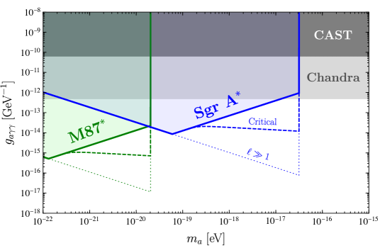
Figure 2: The range of axion-photon couplings that can be probed by the birefringence effect of axion stars in black hole images. Here we use M87^∗ and Sgr A^∗ to discuss the detection capabilities, taking the precision of polarimetric measurement as $3^{\circ}$ for both of them. The masses of M87^∗ and Sgr A^∗ are taken to be $6.5\times 10^{9}M_{\odot}$ [114] and $4.2\times 10^{6}M_{\odot}$ [115] respectively. The shaded parameter space shows the sensitivity by considering axion star formation from gravity only. In the region where $m_{a}$ is relatively small, $t_{H}<t_{\text{decay}}$ and the solid lines obey $g_{a\gamma\gamma}\propto m_{a}^{-3/4}$. In the region where $m_{a}$ is large, $t_{H}>t_{\text{decay}}$, from which we have $g_{a\gamma\gamma}\propto m_{a}^{3/4}$. The dashed "critical" curve encloses the parameter space expanded by including the formation rate from self-interactions where $f_{a}$ is chosen to form critical stars that maximize $\Delta\phi_{\text{polar}}$. The parameter space above the dotted curve shows the potential maximal sensitivity when the decay rate of axion stars $\Gamma\propto(GM_{\text{BH}}m_{a})^{5+4\ell}$ is suppressed for excited states with large $\ell$.

.

II.2 Axion Star Formation at Halo Center

Axions, originally unbound from each other, can form axion stars near black holes in the presence of self-scattering in dense environments. The consequence of axion star formation will populate dense axion clouds around supermassive black holes as gravitational atoms since the SMBH will accrete and absorb the axion star formed in the galactic center [116]. In our work, the enhancement in the axion star formation rate from BHs is not considered. In the following, we will study the formation rate of axion stars in NFW halos and determine the axion field value. The relevant timescale in this problem is the scattering timescale between axions as wave-like particles, which approximately gives the condensation timescale of axion stars in simulations of axion fields. If we consider both gravity and self-interaction, the condensation time scale is [97]

$$\tau=\frac{\tau_{\rm self}\tau_{\text{gr}}}{\tau_{\text{gr}}+\tau_{\rm self}}.$$ (22)

The gravitational condensation time is given by

$$\tau_{\text{gr}}=\frac{b}{48\pi^{3}}\frac{m_{a}^{3}v^{6}}{G_{N}^{2}\rho_{a}^{2}\log\left(m_{a}vR\right)}~{},$$ (23)

and the self-interaction condensation time is

$$\begin{aligned} \tau_{\rm self}=\frac{64dm_{a}^{7}v^{2}}{3\pi\rho_{a}^{2}\lambda^{2}}~{}.\end{aligned}$$ (24)

The parameters $b,d\sim\mathcal{O}(1)$ are numerical coefficients extracted from numerical simulations [117]. In this work, we focus on the scenario where the axion self-coupling strength is given by $\lambda=m_{a}^{2}/f_{a}^{2}$. These are standard formulas that calculate the relaxation scale of axion gas with a given velocity distribution and agree surprisingly well with the axion star formation timescale found in numerical simulations [95, 96, 97, 98]. The velocities and densities should be calculated from halo parameters. Since the halo central density is higher and the velocity is smaller than the halo outskirts, axion star formation rate will be enhanced compared to the halo outskirts. In the post-inflationary scenario of axions, axion miniclusters will form in early times and evolve with time [118], greatly enhancing the axion star formation rate subject to the disruption effect of axion miniclusters in galaxies [119, 120]. Here we do not consider the enhancement from axion miniclusters but focus on the axion star formation in the standard massive dark matter halos. We considered the halo density in the region where the enclosed dark matter mass is the same as the black hole mass, which characterizes the halo environment in the vicinity of supermassive black holes. The detailed calculations are presented in Appendix. D. The characteristic mass scale of axion star can be estimated by equating the virial velocity of the axion star and the halo velocity, which gives [95, 96]

$$\overline{M}_{*}\approx\frac{3\,v}{G_{N}m_{a}}$$ (25)

where $v$ is the velocity of axion waves in dark matter halos. The mass growth of axion stars is found to exhibit a power-law growth after the initial thermalization

$$M_{*}(t)=\overline{M}_{*}\left(\frac{t}{\tau}\right)^{1/2},$$ (26)

where $\tau$ is the condensation time scale given in Eq. 22. It is still debatable if such power-law growth can be extrapolated to masses $M\gg\overline{M_{*}}$ [96, 121]. However, for the parameter space of interest in this paper, the axion stars we are considering are very light and within the mass range where the power law growth is applicable. Since the ground state of the gravitational atom can be absorbed by black holes, one should also include the decay time, $t_{\rm decay}$, of axion star solutions near black holes [122, 123, 124]. The lifetime of axion stars in the ground state is much shorter than those in excited states. Since we do not have a population analysis for the occupancy number of different eigenstates, we assume all the axion stars are in the ground state, which will be the conservative limit. If the lifetime of ground state $t_{\rm decay}$ is much shorter than Hubble time $t_{H}$, one could determine the axion star mass using

$$\begin{aligned} M_{*}\simeq\overline{M}_{*}\,\left(\frac{t_{\rm decay}}{\tau}\right)^{1/2}\,\end{aligned}$$ (27)

If $t_{H}$ is smaller than $t_{\text{decay}}$, we replace $t_{\text{decay}}$ in Eq. (27) by $t_{H}$. It is worth emphasizing again that we use the standard formation rate for the axion stars in the galactic center, which should be a conservative calculation. The axion star itself can help capture more axions [111] and the BH may enhance the accretion rate of axions.

III Axion Sensitivities from black hole polarimetry

Now we will apply our previous calculations to obtain the sensitivity of black hole polarimetry to axion dark matter. Using the axion star mass, one can derive the sensitivity on $g_{a\gamma}$ with the formula in Eq. (17). The axion parameter space that can be probed by the polarimetric measurements of M87^∗ and Sgr A^∗ is presented in Fig. 2. The sensitivity of EHT observations on the polarization angle rotation is taken as 3^∘. There are two competing effects that determine the sensitivities. In general, a large star formation rate will lead to heavier critical axion stars, which provides better sensitivities to lighter axions due to the large Bose enhancements. The decay of axion stars near black holes should also be taken into account, which suppresses the sensitivities when $GM_{\rm BH}m_{a}$ is close to 1. On the other hand, a larger value $GM_{\rm BH}m_{a}$ corresponds to more enhancements on the axion field value of critical stars, which tends to make the sensitivities better. Therefore, we see the sensitivity is almost flattened in a wide range of axion masses, as shown in Fig. 2. Note that the axion decay constant $f_{a}$ is also a crucial part of the story to calculate the axion parameter space that can be probed. A large self-interaction can enhance the formation rate of axion stars, which can expand the discovery space for axion parameters until the critical mass of axion stars is reached, as shown in Fig. 2. But axion star formation can happen even without self-interactions, which will give us the most conservative estimation in the sensitivity to axion parameters from black hole polarimetry, as shown in the shaded region of Fig. 2.

The black hole polarimetry has to resolve the size of the axion star for probing the polarization rotation induced by axion stars. It is challenging to resolve the near horizon region of supermassive black holes if they are at high redshifts. The required angular resolution to probe axions is given by $\sim R_{*}/D_{s}$ where $R_{*}$ is the axion star radius given in Eq. (11) and $D_{s}$ is the comoving distance of the supermassive black hole. Space interferometry in the future will provide a better angular resolution with longer baselines [125], which can resolve axion stars near supermassive black holes much more precisely. Therefore, we expect polarimetric imaging of the near horizon region of supermassive black holes will also serve as competitive axion searches in the future, with great potential to discover axion dark matter.

IV Conclusion

In this work, we systematically study the axion star configuration, axion star formation rate, and the axion birefringence effect around supermassive black holes and propose black hole polarimetry as sensitive axion dark matter detectors. The axion birefringence effect is distinguishable from astrophysical effects on the rotation of polarization angle since it is frequency-independent and modulating at the time scale of $1/m_{a}$ coherently over the size of an axion star. Therefore, if a large axion field value is developed around supermassive black holes, it will become a potential discovery machine for axion dark matter. In our study, a new stable solution of axion stars in the gravitational background of black holes is obtained, and the axion star mass is calculated based on the condensation timescale of axion waves considering both gravitational and axionic self-couplings, showing that a large axion field around black holes is indeed possible for a broad range of parameter space. The maximal mass of axion stars is determined by the axion self-coupling, where a stronger self-coupling corresponds to a smaller maximal mass and larger axion star formation rate. We studied the axion star formation rate using analytical models motivated by numerical simulations. The axion star formation rate from gravity is already significant and the self-coupling of axions can further enhance it, expanding the parameter space that can be probed. When the maximal mass of axion stars is achieved with a sufficiently large axion self-coupling but not too strong to reduce the maximum mass, more axion parameters can be probed. The exact law for the growth of the mass of axion stars is still being actively studied and future numerical studies might change the axion star mass predicted in this work. However, our calculation is conservative as we only considered the condensation of axion waves in dark matter halos, which has been extensively studied in the literature. We did not include the possible enhancements in the formation rate from the gravitational potential of black holes. We show that polarimetric imaging of the near-horizon region of supermassive black holes which can resolve the axion star profile will provide sensitive probes to axion-photon couplings. . Future observations with the next-generation Event Horizon Telescope will greatly expand the axion mass range it can probe with more sources and improve the sensitivity on the axion-photon coupling constant $g_{a\gamma\gamma}$ with better measurements on the polarization angle. Black hole polarimetry will be not only interesting in astrophysics but also provide one of the best complimentary searches on the nature of dark matter.

Appendix A Axion Star Configuration in SMBH Background

In this section, we solve the axion star configuration in the SMBH background. In the SMBH background, the axion field obeys the Klein-Gordon in curved spacetime, which is written as

$$\begin{aligned} \frac{1}{\sqrt{-g}}\partial_{\mu}(\sqrt{-g}g^{\mu\nu}\partial_{\nu}a)=-V^{\prime}(a).\end{aligned}$$ (28)

The metric of the SMBH background in the Newtonian limit is

$$\begin{aligned} g_{\mu\nu}=\text{diag}\big{(}1+2\Phi,-(1-2\Phi)-r^{2},-r^{2}\sin^{2}\theta\big{)},\end{aligned}$$ (29)

where $\Phi$ represents the gravitational potential. In Eq. (29), we use the Newtonian approximation because we focus on the region where $r\gg GM_{\text{BH}}$. Neglecting the axion self-interaction, doing the time average, and neglecting the higher order terms, we write Eq. (28) as

$$\begin{aligned} \boldsymbol{\nabla}^{2}\Theta=2\left(m^{2}_{a}\Phi+\frac{m^{2}_{a}-\omega^{2}_{a}}{2}\right)\Theta,\end{aligned}$$ (30)

where the spatial Laplace operator can be written as

$$\begin{aligned} \boldsymbol{\nabla}^{2}=\frac{\partial^{2}}{\partial r^{2}}+\frac{2}{r}\frac{\partial}{\partial r}\end{aligned}$$ (31)

because the axion’s ground state configuration is spherically symmetric.

In the Newtonian limit, the gravitational potential obeys the Poisson equation, i.e., the linearized Einstein equation. Here, we have

$$\begin{aligned} \boldsymbol{\nabla}^{2}\Phi=4\pi G\rho_{\text{tot}},\end{aligned}$$ (32)

where

$$\begin{aligned} \rho_{\text{tot}}=\rho_{*}+\rho_{\rm BH}.\end{aligned}$$ (33)

Here, $\rho_{*}$ denotes the density of the axion star and $\rho_{\text{BH}}$ denotes the density of the black hole. Because we focus on the region where $r\gg GM_{\text{BH}}$, we approximately have

$$\begin{aligned} \rho_{\rm BH}\simeq M_{\text{BH}}\delta^{(3)}(r).\end{aligned}$$ (34)

Because we focus on the situation where $M_{\text{BH}}\gg M_{*}$, after solving Eq. (32), we have

$$\begin{aligned} \Phi\simeq-\frac{GM_{\text{BH}}}{r}.\end{aligned}$$ (35)

After substituting Eq. (35) and imposing the boundary condition $\Theta(r\rightarrow\infty)=0$, we get the ground state solution

$$\begin{aligned} \Theta(r)=\Theta_{0}\exp\left(-GM_{\text{BH}}m_{a}^{2}r\right)\end{aligned}$$ (36)

with the eigenfrequency

$$\begin{aligned} \omega_{a}=m_{a}\sqrt{1-\left(GM_{\text{BH}}m_{a}\right)^{2}}.\end{aligned}$$ (37)

From Eq. (36), we know that the radius of the axion star is $R_{*}\sim 1/GM_{\text{BH}}m_{a}^{2}$. When $r\gg R_{*}$, the axion field decreases exponentially. To be more specific, we define $R_{*}$ to be radius which envelopes $99\%$ of the axion star mass, then we have

$$\begin{aligned} R_{*}=\frac{c_{99}}{GM_{\text{BH}}m_{a}^{2}},\quad\text{where $c_{99}\simeq 4.2$}.\end{aligned}$$ (38)

From Eq. (37), we find that to have a stable axion configuration, we need

$$\begin{aligned} m_{a}\leq\frac{1}{GM_{\text{BH}}},\end{aligned}$$ (39)

otherwise the axion’s oscillation frequency is imaginary which means that the axion is absorbed by the black hole when its size is comparable with the black hole’s event horizon.

Appendix B Axion Star Enery in SMBH Background

In this section, we will do a detailed calculation of the axion star’s energy in SMBH background. The axion’s energy density can be written as

$$\begin{aligned} \rho_{*}=\frac{\omega^{2}_{a}f_{a}^{2}\Theta^{2}}{4}+\frac{f_{a}^{2}}{4}\left(\frac{d\Theta}{dr}\right)^{2}+\frac{m_{a}^{2}f_{a}^{2}\Theta^{2}}{4}-\frac{\lambda f_{a}^{4}\Theta^{4}}{64},\end{aligned}$$ (40)

where we do the time-average over the time-oscillation terms. In Eq. (40), the first term denotes the oscillation energy density, the second term denotes the gradient energy density, the third term denotes the potential energy density from axion’s mass term, and the fourth term denotes the potential energy density from axion’s self-interaction.

Based on the discussion above, the total energy of axion star can be written as

$$\begin{aligned} E^{\text{tot}}_{*}=E^{\text{osc}}_{*}+E^{\text{grad}}_{*}+E^{\text{mass}}_{*}+E^{\lambda}_{*}+E^{\text{grav}}_{*}.\end{aligned}$$ (41)

Each term in Eq. (41) can be written as

$$\left\{\begin{aligned} &E_{*}^{\text{osc}}=\int d^{3}\boldsymbol{r}\,\frac{\omega_{a}^{2}f_{a}^{2}\Theta^{2}}{4}=\frac{\pi f_{a}^{2}\omega_{a}^{2}\Theta_{0}^{2}}{4G^{3}m_{a}^{6}M_{\text{BH}}^{3}}\\ &E_{*}^{\text{grad}}=\int d^{3}\boldsymbol{r}\,\frac{f_{a}^{2}}{4}\left(\frac{d\Theta}{dr}\right)^{2}=\frac{\pi f_{a}^{2}\Theta_{0}^{2}}{4Gm_{a}^{2}M_{\text{BH}}}\\ &E_{*}^{\text{mass}}=\int d^{3}\boldsymbol{r}\,\frac{m_{a}^{2}f_{a}^{2}\Theta^{2}}{4}=\frac{\pi f_{a}^{2}\Theta_{0}^{2}}{4G^{3}m_{a}^{4}M_{\text{BH}}^{3}}\\ &E_{*}^{\lambda}=-\int d^{3}\boldsymbol{r}\,\frac{\lambda f_{a}^{4}\Theta^{4}}{64}=-\frac{\pi\lambda f_{a}^{4}\Theta_{0}^{4}}{512G^{3}m_{a}^{6}M_{\text{BH}}^{3}}\\ &E_{*}^{\text{grav}}=-\int d^{3}\boldsymbol{r}\,\frac{GM_{\text{BH}}\rho_{*}}{r}\simeq-\frac{\pi f_{a}^{2}\Theta_{0}^{2}}{2Gm_{a}^{2}M_{\text{BH}}}\end{aligned}\right..$$ (42)

When $GM_{\text{BH}}m_{a}\ll 1$, $\omega_{a}\simeq m_{a}$, therefore we have

$$\begin{aligned} M_{*}\simeq E^{\text{osc}}_{*}+E^{\text{mass}}_{*}\simeq\frac{\pi\Theta_{0}^{2}f_{a}^{2}}{2G^{3}M_{\text{BH}}^{3}m_{a}^{4}},\end{aligned}$$ (43)

where contributions from $E^{\text{grad}}_{*}$ and $E^{\lambda}_{*}$ are negligible. Representing $\Theta_{0}$ in terms of $M_{*}$ using Eq. (43), we can write the gradient energy listed in Eq. (42) as

$$\begin{aligned} E^{\text{grad}}_{*}\simeq\frac{Gm_{a}^{2}M_{\text{BH}}^{2}M_{*}}{2}.\end{aligned}$$ (44)

Similarly, we can write the self-interaction energy listed in Eq. (42) as

$$\begin{aligned} E^{\lambda}_{*}\simeq\frac{\lambda\,G^{3}m_{a}^{2}M_{\text{BH}}^{3}M_{*}^{2}}{128\pi},\end{aligned}$$ (45)

and the gravitational energy listed in Eq. (42) as

$$\begin{aligned} E_{*}^{\text{grav}}\simeq-G^{2}m_{a}^{2}M_{\text{BH}}^{2}M_{*}.\end{aligned}$$ (46)

Substituting Eq. (43) into the equation $\Delta\phi_{\text{polar}}\simeq g_{a\gamma\gamma}\Theta_{0}f_{a}/2$, we have

$$\begin{aligned} \Delta\phi_{\text{polar}}\simeq g_{a\gamma\gamma}\left(\frac{G^{3}M_{\text{BH}}^{3}m_{a}^{4}M_{*}}{2\pi}\right)^{1/2}.\end{aligned}$$ (47)

Substituting Eq. (20) into Eq. (47), we can write the rotation angle of the light polarization at the critical mass as

$$\begin{aligned} \Delta\phi^{\max}_{\text{polar}}\simeq\frac{4}{\sqrt{3}}\,g_{a\gamma\gamma}f_{a}\,GM_{\text{BH}}m_{a}.\end{aligned}$$ (48)

Therefore if axions with larger $f_{a}$ can form axion stars at critical masses, the polarization rotation angle will be larger.

Appendix C Critical Mass of the Axion Star in SMBH Background

In this section, we derive the axion star’s critical mass $M_{*}^{\max}$ in the SMBH background with $M_{*}\ll M_{\text{BH}}$ based on the variation principle. Here we have the energy of the axion star, i.e.,

$$\begin{aligned} E_{*}=c_{1}\frac{M_{*}}{2m_{a}^{2}R_{*}^{2}}-c_{2}\frac{\lambda M_{*}^{2}}{12m_{a}^{4}R_{*}^{3}}-c_{3}\frac{GM_{*}M_{\text{BH}}}{R_{*}},\end{aligned}$$ (49)

where the first term is the gradient energy, the second term is the energy from the axion self-interaction, the third term is the gravitational energy of the axion star in the SMBH background. Comparing Eq. (49) with Eq. (38), Eq. (44), Eq. (45), and Eq. (46), we can determine that

$$\begin{aligned} c_{1}=c_{99}^{2},\,c_{2}=\frac{3c_{99}^{3}}{32\pi},\,c_{3}=c_{99}.\end{aligned}$$ (50)

It is worth noting that the numerical values of $c_{1}$, $c_{2}$ in Eq. (50) are different from self-gravitating axion stars where $c_{1}\simeq 9.9$, $c_{2}\simeq 0.85$ [102, 126, 127].

Doing the variation of Eq. (49) and imposing the condition $dE_{*}/dR_{*}=0$ for the configuration’s stability, we have

$$\begin{aligned} R_{*}=\frac{c_{1}}{2c_{3}GM_{\text{BH}}m_{a}^{2}}\left[1\pm\sqrt{1-\frac{c_{2}c_{3}}{c_{1}^{2}}\lambda GM_{*}M_{\text{BH}}}\right].\end{aligned}$$ (51)

In the weak coupling limit where $\lambda$ is negligible, we have $R_{*}\simeq c_{99}/GM_{\text{BH}}m_{a}^{2}$. This is consistent with the result in Eq. (38). However, the axion star is unstable and starts to explode if $M_{*}$ becomes too large. If the axion star stays in a stable configuration, $R_{*}$ in Eq. (51) has to be a real number. This requires that

$$\begin{aligned} M_{*}\leq M_{*}^{\max}=\frac{32\pi}{3\lambda GM_{\text{BH}}}.\end{aligned}$$ (52)

During the axion accretion around the SMBH, the axion star’s mass grows as $M_{*}\propto t^{1/2}$ until $M_{*}\simeq M_{*}^{\max}$. Afterward, the axion star triggers bosenova and maintains a mass $\sim M_{*}^{\max}$. After the Bosenova, the axion field value is only changed by an $\mathcal{O}(1)$ factor, so the conclusion will not be changed qualitatively.

Before ending this section, we want to comment on the different $M_{*}\text{-}R_{*}$ relation for the axion star in the SMBH background and the self-gravitating axion star. As shown in Eq. 51, the black hole mass replaces the axion star mass in the usual axion star mass-radius relation. This is easily understandable because the gravitational potential of axion stars is more important in self-gravitating axion stars while the gravity of black holes is dominating in our case. Therefore, the gravitational potential of black holes naturally holds the axion stars, and axion stars become more compact from the gravitational pull of black holes.

Appendix D Axion Accretion in SMBH Background

Figure 3: The axion parameter space that leads to the formation of axion stars at critical masses near the supermassive black holes is plotted. A smaller $f_{a}$ is ideal for forming critical stars because the formation rate of axion stars is enhanced with a small $f_{a}$ and the corresponding critical mass of axion star is also small. However, it is not required to obtain the sensitivity since axion stars can also form with gravitational interactions. We again considered axion star formation near both M87^∗ and Sgr A^∗. The light gray region is the axion parameter space excluded by the superradiance of SMBHs [34, 35, 36]. Ultralight axion dark matter with masses lighter than $10^{-21}\,\text{eV}$ is excluded by Lyman-$\alpha$ forest [128, 129, 130, 131, 132, 133]. The ultra-faint dwarf galaxies may also place a limit on the dark matter mass to be heavier than $10^{-19}\text{eV}$ [60]. The gray region on the upper left corner shows the constraints from structure formation [134, 135, 136, 111].

In this section, we discuss the accretion of the axion within the background of the SMBH. Axion mass accumulates around the SMBH obeying the power law growth. This effect leads to the mass growth of the axion star. In the meantime, because the part of the axion star inside the horizon of the SMBH is absorbed, it experiences exponential decay. Considering these two competing effects, we have

$$\begin{aligned} \frac{dM_{*}}{dt}=\frac{\overline{M}^{2}_{*}}{\tau}\frac{1}{M_{*}}-M_{*}\Gamma_{\text{decay}},\end{aligned}$$ (53)

where $M_{*}$ begins to evolve from zero to nonzero values at $t=0$. In the right-hand side of Eq. (53), the first term represents the accumulation of axions obeying the power law $M_{*}(t)\propto t^{1/2}$. $\tau$ represents axion’s relaxation time including both the gravitational interaction and the self-interaction. $\overline{M}_{*}$ is the characteristic mass of the axion star. The second term represents the exponential decay of the axion star in the gravitational field of SMBH, which appears as the imaginary part of the energy eigenvalue. From [122, 123, 124], we know that the decay rate is

$$\begin{aligned} \Gamma_{\text{decay}}\sim(m_{a}\Omega_{\text{BH}}-\omega_{a})\times(GM_{\text{BH}}m_{a})^{5+4\ell},\end{aligned}$$ (54)

where $\Omega_{\text{BH}}$ is the spin of the black hole, $\ell$ is the angular momentum quantum number, and $\omega_{a}$ is the real part of the axion oscillation frequency $\omega_{a}=m_{a}\sqrt{1-\left(GM_{\text{BH}}m_{a}\right)^{2}}$. Because we focus on the region where $m_{a}\ll 1/GM_{\text{BH}}$, there is $\omega_{a}\simeq m_{a}$. For the axion star in the ground state, we have $\ell=0$, therefore the inverse of the decay time is

$$\begin{aligned} t_{\text{decay}}^{-1}\sim m_{a}\times(GM_{\text{BH}}m_{a})^{5}.\end{aligned}$$ (55)

During the universe’s evolution, the mass of an axion star grows over time with a power law until the two terms in the left-hand side of Eq. (53) cancel with each other. Given that the age of the universe is $t_{H}\simeq 1/H_{0}$, today’s axion star mass is

$$\begin{aligned} M_{*}=\overline{M}_{*}\times\left(\frac{\min(t_{\text{decay}},t_{H})}{\tau}\right)^{1/2}\end{aligned}$$ (56)

before $M_{*}$ reaches the critical mass $M_{*}^{\max}$.

To calculate $\tau$ in Eq. (56), we need to know $\rho_{a}$. To specify this, we choose $\rho_{a}$ to be the energy density at $r=r_{0}$, where $r_{0}$ satisfies

$$\begin{aligned} M_{\text{halo}}(r<r_{0})\simeq M_{\text{BH}}.\end{aligned}$$ (57)

In the region where $r>r_{0}$, the SMBH’s gravitational field is subdominant, therefore the axions in this region do not feel the existence of SMBH. Moreover, because the axion accretion time mostly depends on the outside mass shell, therefore using $\rho_{a}$ at $r=r_{0}$ is a conservative approach.

We assume that the axion halo has the NFW profile

$$\begin{aligned} \rho_{\text{NFW}}(r)=\frac{\rho_{s}}{\frac{r}{r_{s}}\left(1+\frac{r}{r_{s}}\right)^{2}}.\end{aligned}$$ (58)

If the halo mass integration is cut-off at $r_{200}$, where $r_{200}$ is the radius where the averaged halo density is $200$ times of the average matter density $\rho_{m}$, we have

$$\begin{aligned} \rho_{s}=\frac{\Delta_{200}\rho_{m}c^{3}}{3f(c)}\,\,\,\,\,\text{and}\,\,\,\,\,r_{s}=\left(\frac{M_{\text{halo}}}{4\pi\rho_{s}f(c)}\right)^{1/3},\end{aligned}$$ (59)

where

$$\begin{aligned} f(c)=\log(1+c)-\frac{c}{1+c},\end{aligned}$$ (60)

and $\Delta_{200}=200$. Here, $c$ is the DM halo’s concentration factor and is generally chosen to be $c\sim 10$. To solve $r_{0}$, we substitute Eq. (59) and Eq. (60) into Eq. (57), and then do the Talyor expansion over $r_{0}/r_{s}$ given that $r_{0}\ll r_{s}$. After some algebra, we have

$$\begin{aligned} r_{0}\simeq\left(\frac{M_{\text{BH}}}{2\pi r_{s}\rho_{s}}\right)^{1/2}.\end{aligned}$$ (61)

We also have that

$$\begin{aligned} v_{0}=\left(\frac{2GM_{\text{BH}}}{r_{0}}\right)^{1/2}\end{aligned}$$ (62)

and

$$\begin{aligned} \rho_{0}=\frac{\rho_{s}}{\frac{r_{0}}{r_{s}}\left(1+\frac{r_{0}}{r_{s}}\right)^{2}}.\end{aligned}$$ (63)

Substituting Eq. (63) and Eq. (62) into the formula of the condensation timescale, we will be able to calculate the axion star formation rate. For example, the condensation timescale caused by self-interactions can be expressed as

$$\begin{aligned} \tau_{\rm self}\simeq\frac{64dm_{a}^{3}f_{a}^{4}v^{2}_{0}}{3\pi\rho_{0}^{2}}.\end{aligned}$$ (64)

The gravitational condensation time is given by

$$\tau_{\text{gr}}\simeq\frac{b}{48\pi^{3}}\frac{m_{a}^{3}v^{6}_{0}}{G^{2}\rho^{2}_{0}\log\left(m_{a}v_{0}R\right)}~{}.$$ (65)

Based on Eq. (56) and Eq. (65), we can explain the power law behavior of the solid lines in Fig. 2, where the gravitational condensation dominates. When $m_{a}$ is small, the decay rate is suppressed, which leads to $t_{H}<t_{\text{decay}}$. Thus we have $M_{*}\simeq\overline{M}_{*}(t_{H}/\tau_{\text{gr}})^{1/2}\propto m_{a}^{-5/2}$. Because $\rho_{*}\sim M_{*}/R_{*}^{3}$, we have $\Delta\phi_{\text{polar}}\propto g_{a\gamma\gamma}m_{a}^{3/4}$. Given the determined $\Delta\phi_{\text{polar}}$, we conclude that the solid contours obey $g_{a\gamma\gamma}\propto m_{a}^{-3/4}$. When $t_{\text{decay}}<t_{H}$, we have $M_{*}\simeq\overline{M}_{*}(t_{\text{decay}}/\tau_{\text{gr}})^{1/2}$. From Eq. (55), we have $t_{\text{decay}}\propto m_{a}^{-6}$, which leads to $M_{*}\propto m_{a}^{-11/2}$. Therefore, we have $\Delta\phi_{\text{polar}}\propto g_{a\gamma\gamma}m_{a}^{-3/4}$, from which we have $g_{a\gamma\gamma}\propto m_{a}^{3/4}$.

It is worth noting that the gravitational interaction will dominate over self-interaction if $f_{a}>M_{\rm pl}\,v$ during the formation of axion stars. Also note that the power law growth $M_{*}(t)\propto t^{1/2}$ is only a benchmark model and the power law index may be different. For example, the halo profile may contribute to the power law growth. If a star is formed within a small radius of the halo, which is the situation here, the mass contained in this region is small. For an NFW profile, the mass contained within $r$ is

$$\begin{aligned} M(r)|_{r\rightarrow 0}=4\pi\rho_{s}r_{s}^{3}f(r/r_{s})\simeq 2\pi\rho_{s}r_{s}r^{2}.\end{aligned}$$ (66)

At a small radius, the mass enclosed will form an axion star when all the axion waves are scattered with each other and thermalized. The formation timescale dominated by self-interactions is $\tau_{\rm self}\propto v^{2}/\rho^{2}$. At a small radius of an NFW halo, the dark matter density and velocity scale as $\rho\propto 1/r$ and $v\propto\sqrt{r}$. Therefore, $M(t)\propto r^{2}\propto t^{2/3}$. Similarly, if gravity dominates the axion star formation, $\tau_{gr}\propto v^{6}/\rho^{2}\propto r^{5}$ at a small radius and the mass growth power law is given by $M(t)\propto t^{2/5}$. One may use a different power law index for the growth behavior of axion stars but this should not change the result significantly.

In Ref. [111], the growth of axion stars is further enhanced by the axion star itself since it will capture axions that are originally unbound, triggering exponential growth on the axion star mass before it reaches the critical mass. Such capture rate may not be relevant in our case since the dark matter environment is so dense and the scattering of axion waves is already significant enough to form axion stars. As shown in Eq. 53, the growth term from external axion scattering is $\overline{M_{*}}^{2}/(\tau{M_{*}})$ while axion star capture will introduce a new growth term $M_{*}/\tau$, which is subdominant when $M_{*}<\overline{M_{*}}$.

In Fig. 3, we plot the $m_{a}\text{-}f_{a}$ plane that leads to the formation of critical stars near supermassive black holes. Both $m_{a}$ and $f_{a}$ are relevant for the formation and growth of axion stars as well as their critical mass. When the critical mass is reached, the sensitivity to axion-photon couplings is maximized. It is worth noting that our calculation has been conservative because we considered the decay of axion stars near black holes using the decay rate of axion stars in the ground state. The large decay rate of axion stars when $GM_{\rm BH}m_{a}\sim 1$ is the reason why a small $f_{a}$ is needed to form critical stars at the high mass end. Future simulations of axion fields might be able to determine the exact axion state distributions and we will have a better understanding of the axion parameter space that leads to the formation of critical stars.

References

- Peccei and Quinn [1977] R. D. Peccei and H. R. Quinn, Phys. Rev. Lett. 38, 1440 (1977).
- Weinberg [1978] S. Weinberg, Phys. Rev. Lett. 40, 223 (1978).
- Wilczek [1978] F. Wilczek, Phys. Rev. Lett. 40, 279 (1978).
- Kim [1979] J. E. Kim, Phys. Rev. Lett. 43, 103 (1979).
- Abbott and Sikivie [1983] L. F. Abbott and P. Sikivie, Phys. Lett. B 120, 133 (1983).
- Dine and Fischler [1983] M. Dine and W. Fischler, Phys. Lett. B 120, 137 (1983).
- Preskill et al. [1983] J. Preskill, M. B. Wise, and F. Wilczek, Phys. Lett. B 120, 127 (1983).
- Peccei [2008] R. D. Peccei, Lect. Notes Phys. 741, 3 (2008), arXiv:hep-ph/0607268 .
- Arvanitaki et al. [2010] A. Arvanitaki, S. Dimopoulos, S. Dubovsky, N. Kaloper, and J. March-Russell, Phys. Rev. D 81, 123530 (2010), arXiv:0905.4720 [hep-th] .
- Sikivie et al. [2014] P. Sikivie, N. Sullivan, and D. B. Tanner, Phys. Rev. Lett. 112, 131301 (2014), arXiv:1310.8545 [hep-ph] .
- Kahn et al. [2016] Y. Kahn, B. R. Safdi, and J. Thaler, Phys. Rev. Lett. 117, 141801 (2016), arXiv:1602.01086 [hep-ph] .
- Ouellet et al. [2019] J. L. Ouellet et al., Phys. Rev. Lett. 122, 121802 (2019), arXiv:1810.12257 [hep-ex] .
- Gramolin et al. [2021] A. V. Gramolin, D. Aybas, D. Johnson, J. Adam, and A. O. Sushkov, Nature Phys. 17, 79 (2021), arXiv:2003.03348 [hep-ex] .
- Salemi et al. [2021] C. P. Salemi et al., Phys. Rev. Lett. 127, 081801 (2021), arXiv:2102.06722 [hep-ex] .
- Zhang et al. [2022] Z. Zhang, D. Horns, and O. Ghosh, Phys. Rev. D 106, 023003 (2022), arXiv:2111.04541 [hep-ex] .
- Brouwer et al. [2022] L. Brouwer et al. (DMRadio), Phys. Rev. D 106, 112003 (2022), arXiv:2203.11246 [hep-ex] .
- Jaeckel and Ringwald [2008] J. Jaeckel and A. Ringwald, Phys. Lett. B 659, 509 (2008), arXiv:0707.2063 [hep-ph] .
- Ehret et al. [2009] K. Ehret et al. (ALPS), Nucl. Instrum. Meth. A 612, 83 (2009), arXiv:0905.4159 [physics.ins-det] .
- Caspers et al. [2009] F. Caspers, J. Jaeckel, and A. Ringwald, JINST 4, P11013, arXiv:0908.0759 [hep-ex] .
- Ehret et al. [2010] K. Ehret et al., Phys. Lett. B 689, 149 (2010), arXiv:1004.1313 [hep-ex] .
- Redondo and Ringwald [2011] J. Redondo and A. Ringwald, Contemp. Phys. 52, 211 (2011), arXiv:1011.3741 [hep-ph] .
- Bähre et al. [2013] R. Bähre et al., JINST 8, T09001, arXiv:1302.5647 [physics.ins-det] .
- Betz et al. [2013] M. Betz, F. Caspers, M. Gasior, M. Thumm, and S. W. Rieger, Phys. Rev. D 88, 075014 (2013), arXiv:1310.8098 [physics.ins-det] .
- Ballou et al. [2015] R. Ballou et al. (OSQAR), Phys. Rev. D 92, 092002 (2015), arXiv:1506.08082 [hep-ex] .
- Janish et al. [2019] R. Janish, V. Narayan, S. Rajendran, and P. Riggins, Phys. Rev. D 100, 015036 (2019), arXiv:1904.07245 [hep-ph] .
- Berlin et al. [2020] A. Berlin, R. T. D’Agnolo, S. A. R. Ellis, C. Nantista, J. Neilson, P. Schuster, S. Tantawi, N. Toro, and K. Zhou, JHEP 07 (07), 088, arXiv:1912.11048 [hep-ph] .
- Berlin et al. [2021] A. Berlin, R. T. D’Agnolo, S. A. R. Ellis, and K. Zhou, Phys. Rev. D 104, L111701 (2021), arXiv:2007.15656 [hep-ph] .
- Gao and Harnik [2021] C. Gao and R. Harnik, JHEP 07, 053, arXiv:2011.01350 [hep-ph] .
- Berlin et al. [2022] A. Berlin et al., (2022), arXiv:2203.12714 [hep-ph] .
- DeRocco and Hook [2018] W. DeRocco and A. Hook, Phys. Rev. D 98, 035021 (2018), arXiv:1802.07273 [hep-ph] .
- Obata et al. [2018] I. Obata, T. Fujita, and Y. Michimura, Phys. Rev. Lett. 121, 161301 (2018), arXiv:1805.11753 [astro-ph.CO] .
- Liu et al. [2019] H. Liu, B. D. Elwood, M. Evans, and J. Thaler, Phys. Rev. D 100, 023548 (2019), arXiv:1809.01656 [hep-ph] .
- Fedderke et al. [2023] M. A. Fedderke, J. O. Thompson, R. Cervantes, B. Giaccone, R. Harnik, D. E. Kaplan, S. Posen, and S. Rajendran, (2023), arXiv:2304.11261 [hep-ph] .
- Baryakhtar et al. [2021] M. Baryakhtar, M. Galanis, R. Lasenby, and O. Simon, Phys. Rev. D 103, 095019 (2021), arXiv:2011.11646 [hep-ph] .
- Mehta et al. [2020] V. M. Mehta, M. Demirtas, C. Long, D. J. E. Marsh, L. Mcallister, and M. J. Stott, (2020), arXiv:2011.08693 [hep-th] .
- Ünal et al. [2021] C. Ünal, F. Pacucci, and A. Loeb, JCAP 05, 007, arXiv:2012.12790 [hep-ph] .
- Fox et al. [2023] P. J. Fox, N. Weiner, and H. Xiao, (2023), arXiv:2302.00685 [hep-ph] .
- Mirizzi et al. [2005] A. Mirizzi, G. G. Raffelt, and P. D. Serpico, Phys. Rev. D 72, 023501 (2005), arXiv:astro-ph/0506078 .
- Mirizzi et al. [2009] A. Mirizzi, J. Redondo, and G. Sigl, JCAP 08, 001, arXiv:0905.4865 [hep-ph] .
- Tashiro et al. [2013] H. Tashiro, J. Silk, and D. J. E. Marsh, Phys. Rev. D 88, 125024 (2013), arXiv:1308.0314 [astro-ph.CO] .
- Mukherjee et al. [2018] S. Mukherjee, R. Khatri, and B. D. Wandelt, JCAP 04, 045, arXiv:1801.09701 [astro-ph.CO] .
- Chang et al. [2023] J. H. Chang, R. Ebadi, X. Luo, and E. H. Tanin, Phys. Rev. D 108, 075013 (2023), arXiv:2305.03749 [hep-ph] .
- Wouters and Brun [2013] D. Wouters and P. Brun, Astrophys. J. 772, 44 (2013), arXiv:1304.0989 [astro-ph.HE] .
- Marsh et al. [2017] M. C. D. Marsh, H. R. Russell, A. C. Fabian, B. P. McNamara, P. Nulsen, and C. S. Reynolds, JCAP 12, 036, arXiv:1703.07354 [hep-ph] .
- Reynolds et al. [2020] C. S. Reynolds, M. C. D. Marsh, H. R. Russell, A. C. Fabian, R. Smith, F. Tombesi, and S. Veilleux, Astrophys. J. 890, 59 (2020), arXiv:1907.05475 [hep-ph] .
- Dessert et al. [2019] C. Dessert, A. J. Long, and B. R. Safdi, Phys. Rev. Lett. 123, 061104 (2019), arXiv:1903.05088 [hep-ph] .
- Buschmann et al. [2021] M. Buschmann, R. T. Co, C. Dessert, and B. R. Safdi, Phys. Rev. Lett. 126, 021102 (2021), arXiv:1910.04164 [hep-ph] .
- Dessert et al. [2020] C. Dessert, J. W. Foster, and B. R. Safdi, Phys. Rev. Lett. 125, 261102 (2020), arXiv:2008.03305 [hep-ph] .
- Dessert et al. [2022] C. Dessert, A. J. Long, and B. R. Safdi, Phys. Rev. Lett. 128, 071102 (2022), arXiv:2104.12772 [hep-ph] .
- Reynés et al. [2021] J. S. Reynés, J. H. Matthews, C. S. Reynolds, H. R. Russell, R. N. Smith, and M. C. D. Marsh, Mon. Not. Roy. Astron. Soc. 510, 1264 (2021), arXiv:2109.03261 [astro-ph.HE] .
- Mirizzi and Montanino [2009] A. Mirizzi and D. Montanino, JCAP 12, 004, arXiv:0911.0015 [astro-ph.HE] .
- Horns et al. [2012] D. Horns, L. Maccione, A. Mirizzi, and M. Roncadelli, Phys. Rev. D 85, 085021 (2012), arXiv:1203.2184 [astro-ph.HE] .
- Meyer et al. [2013] M. Meyer, D. Horns, and M. Raue, Phys. Rev. D 87, 035027 (2013), arXiv:1302.1208 [astro-ph.HE] .
- Ajello et al. [2016] M. Ajello et al. (Fermi-LAT), Phys. Rev. Lett. 116, 161101 (2016), arXiv:1603.06978 [astro-ph.HE] .
- Meyer et al. [2017] M. Meyer, M. Giannotti, A. Mirizzi, J. Conrad, and M. A. Sánchez-Conde, Phys. Rev. Lett. 118, 011103 (2017), arXiv:1609.02350 [astro-ph.HE] .
- Meyer and Petrushevska [2020] M. Meyer and T. Petrushevska, Phys. Rev. Lett. 124, 231101 (2020), [Erratum: Phys.Rev.Lett. 125, 119901 (2020)], arXiv:2006.06722 [astro-ph.HE] .
- Mastrototaro et al. [2022] L. Mastrototaro, P. Carenza, M. Chianese, D. F. G. Fiorillo, G. Miele, A. Mirizzi, and D. Montanino, Eur. Phys. J. C 82, 1012 (2022), arXiv:2206.08945 [hep-ph] .
- Van Tilburg [2021] K. Van Tilburg, Phys. Rev. D 104, 023019 (2021), arXiv:2006.12431 [hep-ph] .
- DeRocco et al. [2022] W. DeRocco, S. Wegsman, B. Grefenstette, J. Huang, and K. Van Tilburg, Phys. Rev. Lett. 129, 101101 (2022), arXiv:2205.05700 [hep-ph] .
- Dalal and Kravtsov [2022] N. Dalal and A. Kravtsov, Phys. Rev. D 106, 063517 (2022), arXiv:2203.05750 [astro-ph.CO] .
- Wadekar and Wang [2022] D. Wadekar and Z. Wang, Phys. Rev. D 106, 075007 (2022), arXiv:2111.08025 [hep-ph] .
- Wadekar and Wang [2023] D. Wadekar and Z. Wang, Phys. Rev. D 107, 083011 (2023), arXiv:2211.07668 [hep-ph] .
- Dror et al. [2021] J. A. Dror, H. Murayama, and N. L. Rodd, Phys. Rev. D 103, 115004 (2021), [Erratum: Phys.Rev.D 106, 119902 (2022)], arXiv:2101.09287 [hep-ph] .
- Langhoff et al. [2022] K. Langhoff, N. J. Outmezguine, and N. L. Rodd, Phys. Rev. Lett. 129, 241101 (2022), arXiv:2209.06216 [hep-ph] .
- Nitta et al. [2023] T. Nitta et al. (ADMX), Phys. Rev. Lett. 131, 101002 (2023), arXiv:2303.06282 [hep-ex] .
- Hook and Huang [2018] A. Hook and J. Huang, JHEP 06, 036, arXiv:1708.08464 [hep-ph] .
- Balkin et al. [2022] R. Balkin, J. Serra, K. Springmann, S. Stelzl, and A. Weiler, (2022), arXiv:2211.02661 [hep-ph] .
- Huang et al. [2018] F. P. Huang, K. Kadota, T. Sekiguchi, and H. Tashiro, Phys. Rev. D 97, 123001 (2018), arXiv:1803.08230 [hep-ph] .
- Caputo et al. [2018] A. Caputo, C. P. n. Garay, and S. J. Witte, Phys. Rev. D 98, 083024 (2018), [Erratum: Phys.Rev.D 99, 089901 (2019)], arXiv:1805.08780 [astro-ph.CO] .
- Safdi et al. [2019] B. R. Safdi, Z. Sun, and A. Y. Chen, Phys. Rev. D 99, 123021 (2019), arXiv:1811.01020 [astro-ph.CO] .
- Caputo et al. [2019] A. Caputo, M. Regis, M. Taoso, and S. J. Witte, JCAP 03, 027, arXiv:1811.08436 [hep-ph] .
- Raffelt [1986] G. G. Raffelt, Phys. Rev. D 33, 897 (1986).
- Anastassopoulos et al. [2017] V. Anastassopoulos et al. (CAST), Nature Phys. 13, 584 (2017), arXiv:1705.02290 [hep-ex] .
- O’Hare et al. [2020] C. A. J. O’Hare, A. Caputo, A. J. Millar, and E. Vitagliano, Phys. Rev. D 102, 043019 (2020), arXiv:2006.10415 [astro-ph.CO] .
- Harari and Sikivie [1992] D. Harari and P. Sikivie, Phys. Lett. B 289, 67 (1992).
- Fedderke et al. [2019] M. A. Fedderke, P. W. Graham, and S. Rajendran, Phys. Rev. D 100, 015040 (2019), arXiv:1903.02666 [astro-ph.CO] .
- Diego-Palazuelos et al. [2022] P. Diego-Palazuelos et al., Phys. Rev. Lett. 128, 091302 (2022), arXiv:2201.07682 [astro-ph.CO] .
- Ade et al. [2022] P. A. R. Ade et al. (BICEP/Keck), Phys. Rev. D 105, 022006 (2022), arXiv:2108.03316 [astro-ph.CO] .
- Adachi et al. [2023] S. Adachi et al. (POLARBEAR), Phys. Rev. D 108, 043017 (2023), arXiv:2303.08410 [astro-ph.CO] .
- Ferguson et al. [2022] K. R. Ferguson et al. (SPT-3G), Phys. Rev. D 106, 042011 (2022), arXiv:2203.16567 [astro-ph.CO] .
- Agrawal et al. [2020] P. Agrawal, A. Hook, and J. Huang, JHEP 07, 138, arXiv:1912.02823 [astro-ph.CO] .
- Liu et al. [2020] T. Liu, G. Smoot, and Y. Zhao, Phys. Rev. D 101, 063012 (2020), arXiv:1901.10981 [astro-ph.CO] .
- Yuan et al. [2021] G.-W. Yuan, Z.-Q. Xia, C. Tang, Y. Zhao, Y.-F. Cai, Y. Chen, J. Shu, and Q. Yuan, JCAP 03, 018, arXiv:2008.13662 [astro-ph.HE] .
- Jain et al. [2021] M. Jain, A. J. Long, and M. A. Amin, JCAP 05, 055, arXiv:2103.10962 [astro-ph.CO] .
- Yin et al. [2022] W. W. Yin, L. Dai, and S. Ferraro, JCAP 06 (06), 033, arXiv:2111.12741 [astro-ph.CO] .
- Liu et al. [2023] T. Liu, X. Lou, and J. Ren, Phys. Rev. Lett. 130, 121401 (2023), arXiv:2111.10615 [astro-ph.HE] .
- Castillo et al. [2022] A. Castillo, J. Martin-Camalich, J. Terol-Calvo, D. Blas, A. Caputo, R. T. G. Santos, L. Sberna, M. Peel, and J. A. Rubiño Martín, JCAP 06 (06), 014, arXiv:2201.03422 [astro-ph.CO] .
- Yao et al. [2023] R.-M. Yao, X.-J. Bi, J.-W. Wang, and P.-F. Yin, Phys. Rev. D 107, 043031 (2023), arXiv:2209.14214 [astro-ph.HE] .
- Hagimoto and Long [2023] R. Hagimoto and A. J. Long, JCAP 09, 024, arXiv:2306.07351 [astro-ph.CO] .
- Fortin and Sinha [2023] J.-F. Fortin and K. Sinha, JCAP 08, 042, arXiv:2303.17641 [astro-ph.HE] .
- Akiyama et al. [2019a] K. Akiyama et al. (Event Horizon Telescope), Astrophys. J. Lett. 875, L5 (2019a), arXiv:1906.11242 [astro-ph.GA] .
- Goddi et al. [2021] C. Goddi et al. (ALMA), Astrophys. J. Lett. 910, L14 (2021), arXiv:2105.02272 [astro-ph.GA] .
- Kolb and Tkachev [1993] E. W. Kolb and I. I. Tkachev, Phys. Rev. Lett. 71, 3051 (1993), arXiv:hep-ph/9303313 .
- Schive et al. [2014] H.-Y. Schive, M.-H. Liao, T.-P. Woo, S.-K. Wong, T. Chiueh, T. Broadhurst, and W. Y. P. Hwang, Phys. Rev. Lett. 113, 261302 (2014), arXiv:1407.7762 [astro-ph.GA] .
- Levkov et al. [2018] D. G. Levkov, A. G. Panin, and I. I. Tkachev, Phys. Rev. Lett. 121, 151301 (2018), arXiv:1804.05857 [astro-ph.CO] .
- Eggemeier and Niemeyer [2019] B. Eggemeier and J. C. Niemeyer, Phys. Rev. D 100, 063528 (2019), arXiv:1906.01348 [astro-ph.CO] .
- Chen et al. [2022a] J. Chen, X. Du, E. W. Lentz, and D. J. E. Marsh, Phys. Rev. D 106, 023009 (2022a), arXiv:2109.11474 [astro-ph.CO] .
- Chan et al. [2022] J. H.-H. Chan, S. Sibiryakov, and W. Xue, (2022), arXiv:2207.04057 [astro-ph.CO] .
- Glennon et al. [2023] N. Glennon, N. Musoke, and C. Prescod-Weinstein, Phys. Rev. D 107, 063520 (2023), arXiv:2302.04302 [astro-ph.CO] .
- Jain et al. [2023] M. Jain, W. Wanichwecharungruang, and J. Thomas, (2023), arXiv:2310.00058 [astro-ph.CO] .
- Eby et al. [2016a] J. Eby, P. Suranyi, and L. C. R. Wijewardhana, Mod. Phys. Lett. A 31, 1650090 (2016a), arXiv:1512.01709 [hep-ph] .
- Visinelli et al. [2018] L. Visinelli, S. Baum, J. Redondo, K. Freese, and F. Wilczek, Phys. Lett. B 777, 64 (2018), arXiv:1710.08910 [astro-ph.CO] .
- Eby et al. [2019] J. Eby, M. Leembruggen, L. Street, P. Suranyi, and L. C. R. Wijewardhana, Phys. Rev. D 100, 063002 (2019), arXiv:1905.00981 [hep-ph] .
- Chen et al. [2020] Y. Chen, J. Shu, X. Xue, Q. Yuan, and Y. Zhao, Phys. Rev. Lett. 124, 061102 (2020), arXiv:1905.02213 [hep-ph] .
- Chen et al. [2022b] Y. Chen, Y. Liu, R.-S. Lu, Y. Mizuno, J. Shu, X. Xue, Q. Yuan, and Y. Zhao, Nature Astron. 6, 592 (2022b), arXiv:2105.04572 [hep-ph] .
- Chen et al. [2022c] Y. Chen, C. Li, Y. Mizuno, J. Shu, X. Xue, Q. Yuan, Y. Zhao, and Z. Zhou, JCAP 09, 073, arXiv:2208.05724 [hep-ph] .
- Farina et al. [2017] M. Farina, D. Pappadopulo, F. Rompineve, and A. Tesi, JHEP 01, 095, arXiv:1611.09855 [hep-ph] .
- Agrawal et al. [2018] P. Agrawal, J. Fan, M. Reece, and L.-T. Wang, JHEP 02, 006, arXiv:1709.06085 [hep-ph] .
- Banerjee et al. [2020a] A. Banerjee, D. Budker, J. Eby, H. Kim, and G. Perez, Commun. Phys. 3, 1 (2020a), arXiv:1902.08212 [hep-ph] .
- Banerjee et al. [2020b] A. Banerjee, D. Budker, J. Eby, V. V. Flambaum, H. Kim, O. Matsedonskyi, and G. Perez, JHEP 09, 004, arXiv:1912.04295 [hep-ph] .
- Budker et al. [2023] D. Budker, J. Eby, M. Gorghetto, M. Jiang, and G. Perez, (2023), arXiv:2306.12477 [hep-ph] .
- Eby et al. [2016b] J. Eby, M. Leembruggen, P. Suranyi, and L. C. R. Wijewardhana, JHEP 12, 066, arXiv:1608.06911 [astro-ph.CO] .
- Levkov et al. [2017] D. G. Levkov, A. G. Panin, and I. I. Tkachev, Phys. Rev. Lett. 118, 011301 (2017), arXiv:1609.03611 [astro-ph.CO] .
- Akiyama et al. [2019b] K. Akiyama et al. (Event Horizon Telescope), Astrophys. J. Lett. 875, L6 (2019b), arXiv:1906.11243 [astro-ph.GA] .
- GRAVITY Collaboration et al. [2019] GRAVITY Collaboration, R. Abuter, A. Amorim, M. Bauböck, J. P. Berger, H. Bonnet, W. Brandner, Y. Clénet, V. Coudé Du Foresto, P. T. de Zeeuw, J. Dexter, G. Duvert, A. Eckart, F. Eisenhauer, N. M. Förster Schreiber, P. Garcia, F. Gao, E. Gendron, R. Genzel, O. Gerhard, S. Gillessen, M. Habibi, X. Haubois, T. Henning, S. Hippler, M. Horrobin, A. Jiménez-Rosales, L. Jocou, P. Kervella, S. Lacour, V. Lapeyrère, J. B. Le Bouquin, P. Léna, T. Ott, T. Paumard, K. Perraut, G. Perrin, O. Pfuhl, S. Rabien, G. Rodriguez Coira, G. Rousset, S. Scheithauer, A. Sternberg, O. Straub, C. Straubmeier, E. Sturm, L. J. Tacconi, F. Vincent, S. von Fellenberg, I. Waisberg, F. Widmann, E. Wieprecht, E. Wiezorrek, J. Woillez, and S. Yazici, A&A 625, L10 (2019), arXiv:1904.05721 [astro-ph.GA] .
- Davies and Mocz [2020] E. Y. Davies and P. Mocz, Mon. Not. Roy. Astron. Soc. 492, 5721 (2020), arXiv:1908.04790 [astro-ph.GA] .
- Chen et al. [2021] J. Chen, X. Du, E. W. Lentz, D. J. E. Marsh, and J. C. Niemeyer, Phys. Rev. D 104, 083022 (2021), arXiv:2011.01333 [astro-ph.CO] .
- Xiao et al. [2021] H. Xiao, I. Williams, and M. McQuinn, Phys. Rev. D 104, 023515 (2021), arXiv:2101.04177 [astro-ph.CO] .
- Kavanagh et al. [2021] B. J. Kavanagh, T. D. P. Edwards, L. Visinelli, and C. Weniger, Phys. Rev. D 104, 063038 (2021), arXiv:2011.05377 [astro-ph.GA] .
- Shen et al. [2022] X. Shen, H. Xiao, P. F. Hopkins, and K. M. Zurek, (2022), arXiv:2207.11276 [astro-ph.GA] .
- Dmitriev et al. [2023] A. S. Dmitriev, D. G. Levkov, A. G. Panin, and I. I. Tkachev, (2023), arXiv:2305.01005 [astro-ph.CO] .
- Detweiler [1980] S. L. Detweiler, Phys. Rev. D 22, 2323 (1980).
- Baryakhtar et al. [2017] M. Baryakhtar, R. Lasenby, and M. Teo, Phys. Rev. D 96, 035019 (2017), arXiv:1704.05081 [hep-ph] .
- Baumann et al. [2019] D. Baumann, H. S. Chia, J. Stout, and L. ter Haar, JCAP 12, 006, arXiv:1908.10370 [gr-qc] .
- Gurvits et al. [2022] L. I. Gurvits et al., Acta Astronaut. 196, 314 (2022), arXiv:2204.09144 [astro-ph.IM] .
- Ruffini and Bonazzola [1969] R. Ruffini and S. Bonazzola, Phys. Rev. 187, 1767 (1969).
- Membrado et al. [1989] M. Membrado, J. Abad, A. F. Pacheco, and J. Sanudo, Phys. Rev. D 40, 2736 (1989).
- Iršič et al. [2017] V. Iršič, M. Viel, M. G. Haehnelt, J. S. Bolton, and G. D. Becker, Phys. Rev. Lett. 119, 031302 (2017), arXiv:1703.04683 [astro-ph.CO] .
- Kobayashi et al. [2017] T. Kobayashi, R. Murgia, A. De Simone, V. Iršič, and M. Viel, Phys. Rev. D 96, 123514 (2017), arXiv:1708.00015 [astro-ph.CO] .
- Armengaud et al. [2017] E. Armengaud, N. Palanque-Delabrouille, C. Yèche, D. J. E. Marsh, and J. Baur, Mon. Not. Roy. Astron. Soc. 471, 4606 (2017), arXiv:1703.09126 [astro-ph.CO] .
- Zhang et al. [2018] J. Zhang, J.-L. Kuo, H. Liu, Y.-L. S. Tsai, K. Cheung, and M.-C. Chu, Astrophys. J. 863, 73 (2018), arXiv:1708.04389 [astro-ph.CO] .
- Nori et al. [2019] M. Nori, R. Murgia, V. Iršič, M. Baldi, and M. Viel, Mon. Not. Roy. Astron. Soc. 482, 3227 (2019), arXiv:1809.09619 [astro-ph.CO] .
- Rogers and Peiris [2021] K. K. Rogers and H. V. Peiris, Phys. Rev. Lett. 126, 071302 (2021), arXiv:2007.12705 [astro-ph.CO] .
- Arvanitaki et al. [2015] A. Arvanitaki, J. Huang, and K. Van Tilburg, Phys. Rev. D 91, 015015 (2015), arXiv:1405.2925 [hep-ph] .
- Fan [2016] J. Fan, Phys. Dark Univ. 14, 84 (2016), arXiv:1603.06580 [hep-ph] .
- Cembranos et al. [2018] J. A. R. Cembranos, A. L. Maroto, S. J. Núñez Jareño, and H. Villarrubia-Rojo, JHEP 08, 073, arXiv:1805.08112 [astro-ph.CO] .