Bayesian Optimization of Function Networks with Partial Evaluations

Abstract

Bayesian optimization is a framework for optimizing functions that are costly or time-consuming to evaluate. Recent work has considered Bayesian optimization of function networks (BOFN), where the objective function is computed via a network of functions, each taking as input the output of previous nodes in the network and additional parameters. Exploiting this network structure has been shown to yield significant performance improvements. Existing BOFN algorithms for general-purpose networks are required to evaluate the full network at each iteration. However, many real-world applications allow evaluating nodes individually. To take advantage of this opportunity, we propose a novel knowledge gradient acquisition function for BOFN that chooses which node to evaluate as well as the inputs for that node in a cost-aware fashion. This approach can dramatically reduce query costs by allowing the evaluation of part of the network at a lower cost relative to evaluating the entire network. We provide an efficient approach to optimizing our acquisition function and show it outperforms existing BOFN methods and other benchmarks across several synthetic and real-world problems. Our acquisition function is the first to enable cost-aware optimization of a broad class of function networks.

Keywords Bayesian Optimization  $\cdot$ Grey-Box Methods  $\cdot$ Function Networks

1 Introduction

Bayesian optimization (BO) (Močkus,, 1975; Jones et al.,, 1998) has emerged as a versatile framework for optimizing functions with costly or time-consuming evaluations. BO has proved its efficacy in a variety of applications, including hyperparameter tuning of machine learning models (Snoek et al.,, 2012), materials design (Frazier et al.,, 2008; Zhang et al.,, 2020), vaccine manufacturing (Rosa et al.,, 2022), and pharmaceutical product development (Sano et al.,, 2020).

In many applications, such as manufacturing (Ghasemi et al.,, 2018), epidemic model calibration (Garnett,, 2002), machine learning pipeline optimization (Xin et al.,, 2021), or robotic control (Plappert et al.,, 2018), objective functions are often computed by evaluating a network of functions where each function takes as input the outputs of its parent nodes. Consider the function network in Figure 1. It represents the multiple stages of a manufacturing process. The process begins with a raw material described by $x_{1}$. This raw material is used to produce an intermediate part described by $y_{1}$ through a process $f_{1}$. Similarly, a second raw material described by $x_{2}$ is used to produce another intermediate part described by $y_{2}$. The parts (with properties $y_{1}$ and $y_{2}$), together with another raw material described by $x_{3}$, are assembled in a process $f_{3}$ to make the final product, the quality of which is denoted by $y_{3}$. Our goal is to choose $x_{1},x_{2},x_{3}$ to maximize $y_{3}$.

Figure 1: An example function network in the manufacturing problem.

Astudillo and Frazier, 2021a showed that utilizing intermediate outputs in the network, i.e., $y_{1}$ and $y_{2}$, to decide which design parameters $x=(x_{1},x_{2},x_{3})$ to evaluate significantly improves the performance of BO methods. However, this and other prior work has not leveraged the ability to perform partial evaluations of the function network, i.e., the ability to evaluate a subset of nodes in the network and use this information to decide the design variables of subsequent nodes and potentially even to pause the evaluation process. As we shall see later, doing so can significantly boost performance, especially in situations where evaluation cost varies significantly across nodes. To illustrate, suppose that evaluating $f_{1}$ is much cheaper than evaluating $f_{2}$. Then, it may be beneficial to focus our initial resources on understanding the possible range of values taken by $y_{1}$ before making too many evaluations of $f_{2}$.

In this work, we introduce a BO algorithm that outperforms existing methods by taking advantage of the ability to perform partial evaluations. This algorithm iteratively selects a node in the function network and an input at which to evaluate it with the goal of identifying the global optimum within a limited budget.

Our contributions are summarized as follows:

1. We introduce a Bayesian optimization framework for function networks that allow partial evaluations.

2. We propose a knowledge-gradient-based acquisition function (KGFN) that, to our knowledge, is the first to enable partial evaluations in a general function network and in a cost-aware fashion.

3. We propose an approximation of KGFN that can be optimized more efficiently.

4. We demonstrate the benefits of exploiting partial evaluations through several numerical experiments, including both synthetic and real-world applications with a variety of network structures.

1.1 Related Work

Our framework aligns with the concept of grey-box BO (Astudillo and Frazier, 2021b, ), where the objective function is not treated entirely as a black box. Instead, the (known) network structure is utilized to improve sampling decisions. BO of functions with a composite or network structure has been previously considered in the literature. For instance, Uhrenholt and Jensen, (2019) considered objective functions that are a sum of squared errors, while a more general setting where the objective function is the composition of a costly (vector-valued) inner function and a cheap outer function was studied by Astudillo and Frazier, (2019) and Jain et al., (2023). Astudillo and Frazier, 2021a pioneered BO of function networks, introducing a probabilistic model that exploits function network structures. This model was paired with the expected improvement (EI) acquisition function (Jones et al.,, 1998) to produce the first BO method to optimize function networks.

The ability to perform partial evaluations in the context of BO of function networks has been studied for specific network structures. Specifically, Kusakawa et al., (2022) considered function networks constituted by a single chain of nodes and developed an algorithm that can pause an evaluation at an intermediate node. However, their approach, utilizing an EI-based acquisition function, cannot be easily extended to quantify the “benefit” of evaluating a single node in a more general function network. Outside the function networks setting, Hernández-Lobato et al., (2016) and Daulton et al., (2023) considered partial evaluations in constrained and multi-objective BO, respectively.

2 Problem and Statistical Model

2.1 Problem Statement

Following the setup in Astudillo and Frazier, 2021a , we consider a sequence of functions $f_{1},f_{2},\ldots,f_{K}$, arranged as nodes in a network representing the evaluation process. Specifically, the network structure is encoded as a directed acyclic graph $\mathcal{G}=(\mathcal{V},\mathcal{E}),$ where $\mathcal{V}=\{1,2,\ldots,K\}$ and $\mathcal{E}=\{(i,j):f_{j}\text{ takes the output of }f_{i}\text{ as input}\}$ denote the sets of nodes and edges, respectively.

Let $J(k)$ denote node $k$’s parent nodes. We assume, without loss of generality, that nodes are ordered such that $j<k$ for all $j\in J(k)$. We also let $I(k)\subseteq\{1,2,\ldots,d\}$ denote the set of components of the function network’s input vector $x\in\mathbb{X}\subset\mathbb{R}^{d}$ taken as an input by each $f_{k}$. We denote by $y_{k}(x)=f_{k}(z_{k})$ the output of node $k$ under input $x$, where $z_{k}=(y_{J(k)}(x),x_{I(k)})\in\mathbb{Z}_{k}:=\mathbb{Y}_{J(k)}\times\mathbb{X}_{k}$ consists of outputs of node $k$’s parent nodes $y_{J(k)}$ and additional input parameters $x_{I(k)}$. While each $f_{k}$ has the flexibility to be either single-output or multi-output, we constrain the final function node, $f_{K}$ to scalar-valued for simplicity. Nevertheless, our methodology can readily accommodate a vector-valued $f_{K}$.

For each node $k$, we assume that there is an associated known evaluation cost function $c_{k}(\cdot)$. Our goal is to maximize the final node’s function value, i.e., $y_{K}(x)$, while minimizing cumulative cost.

In this work, we focus on networks satisfying the following conditions. These conditions facilitate the derivation of our acquisition function. However, as discussed below, some of these conditions may be relaxed.

Condition 1 (Downstream Evaluation)

Evaluating a node $f_{k}$ at $z_{k}=(y_{J(k)}(x),x_{I(k)})$ requires that outputs from $y_{J(k)}(x)$ be attained beforehand.

Condition 2 (Reusablility)

The outputs of intermediate nodes are reusable, i.e., they can be repeatedly combined with new sets of controllable variables and outputs from other nodes at their child nodes.

Condition 3 (Non-Overlapping)

For any $j>i$, if node $f_{j}$ is not reachable from node $f_{i}$, then $I(i)\cap I(j)=\emptyset$ and $J(i)\cap J(j)=\emptyset$.

These conditions are prevalent in practical scenarios. Taking the manufacturing problem as an example: Condition 1 requires that evaluation of a downstream process rely on obtaining necessary outputs from its upstream processes beforehand. While Condition 2 may not be strictly met in the manufacturing setting, it can be considered as approximately satisfied in scenarios like large batch production. Another example where Condition 2 applies is in machine learning pipeline optimization, where previously fitted models can be saved and reused.

Condition 3 ensures that the evaluation of a downstream node is possible by avoiding situations where a valid combination of parent nodes’ outputs is absent. More precisely, without this condition, it is probable that even if we have evaluations for a node’s parent nodes, these evaluations come from different design points that are incompatible with each other, rendering the evaluation of this downstream node infeasible. In addition, if two function nodes are not reachable from each other, then they are likely not closely related, hence justifying Condition 3.

Our approach can be extended when these conditions are not met. Specifically, when Conditions 1 and 2 are not satisfied, our approach works regardless of whether Condition 3 is satisfied. In fact, in such scenarios, optimizing the acquisition function is even simpler than the routine outlined in Section 4. When only Condition 3 is violated, we hypothesize that our algorithm does not work well, as discussed above.

2.2 Statistical Model

In this work, we model functions $f_{1},f_{2},\ldots,f_{K}$ as being sampled from independent Gaussian process (GP) prior distributions. Let $\mu_{0,k}$ and $\Sigma_{0,k}$ be the prior mean and covariance functions of $f_{k}$, respectively, for $k=1,\ldots,K$. We denote by $\mathcal{D}_{n}$ the collection of past observations evaluated at each node of the function network, i.e., $\mathcal{D}_{n}=\{(z_{j,k},y_{j,k})_{j=1}^{n_{k}}\}_{k=1}^{K}$, where $n_{k}$ is the number of observations at node $k$ and $\sum_{k=1}^{K}n_{k}=n$.

The observations at each node $k$, $\{(z_{j,k},y_{j,k})\}_{j=1}^{n_{k}}$, result in a GP posterior distribution over $f_{k}$ with posterior mean $\mu_{n,k}$ and covariance functions $\Sigma_{n,k}$ which is, again, independent of the posterior GPs associated with other functions in the network. Given any input $z_{k}$ for a node $k$, posterior mean $\mu_{n,k}(z_{k})$ and standard deviation $\sigma_{n,k}(z_{k})=\Sigma_{n,k}(z_{k})^{1/2}$ can be computed in closed form (see Williams and Rasmussen, (2006) for details). The posterior distributions over $f_{1},\ldots,f_{K}$ further imply a posterior distribution of a final node value $y_{K}$. Due to the network structure, the posterior distribution of $y_{K}$ at $x\in\mathbb{X}$ is no longer Gaussian. However, sampling from the posterior can be done efficiently, as we discuss in Section 4.2.

Our acquisition function, formally defined in Section 3, is constructed based on these posterior distributions and evaluation costs $c_{k}(\cdot)$. It quantifies the benefits of performing one additional partial evaluation at a specific node. Our BO algorithm then decides to evaluate at a node $k^{*}$ with input $z^{*}_{k^{*}}$ yielding the maximum value of this acquisition function.

3 The KGFN Acquisition Function

Motivated by our goal to improve the solution quality while minimizing cumulative cost, we aim to decide which node to evaluate and at which input in a cost-effective fashion at each iteration. Let $\nu_{n}(x)$ denote the posterior mean of $y_{K}(x)$ given $\mathcal{D}_{n}$. Assuming risk-neutrality, the solution we would select if we were to stop at time $n$ would be the $x$ that maximizes the posterior mean of the final node’s value, i.e.,

$$\nu^{*}_{n}=\max_{x\in\mathbb{X}}\nu_{n}(x).$$ (1)

Now, suppose one additional evaluation at a single function node is allowed. For a node $k$ with a given input $z_{k}$, observing $f_{k}(z_{k})$ would result in an updated posterior over $f_{k}$, which further yields an updated posterior mean function of the final node value $\nu_{n+1}(\cdot)$ and hence an updated maximum of the final function node’s posterior mean, $\nu_{n+1}^{*}$. The difference between the two quantities, i.e., $\nu^{*}_{n+1}-\nu^{*}_{n}$, measures the increment in the expected solution quality.

Before evaluating $f_{k}(z_{k})$, this increment is a random variable. Taking the expectation of this increment with respect to $y_{k}=f_{k}(z_{k})$ and dividing it by the cost of evaluation $c_{k}(z_{k})$, we formally define our knowledge gradient acquisition function for function networks with partial evaluations (KGFN) by

$$\alpha_{n,k}(z_{k})=\frac{\mathbb{E}_{y_{k}}[\nu_{n+1}^{*}]-\nu_{n}^{*}}{c_{k}(z_{k})}.$$ (2)

This acquisition function aligns with the original knowledge gradient (Frazier et al.,, 2008; Wu and Frazier,, 2016). Moreover, it is cost-ware (in that it favors lower-cost evaluations at the same expected quality) and is similar in nature to the acquisitions proposed in Wu et al., (2020) and Daulton et al., (2023).

In each iteration, our decision is to evaluate at node $k^{*}$ with inputs $z^{*}_{k^{*}}$ such that

$$(k^{*},z^{*}_{k^{*}})\in\operatorname*{arg\,max}_{k\in\{1,\ldots,K\}}\operatorname*{arg\,max}_{z_{k}\in\mathbb{Z}_{k}}\ \alpha_{n,k}(z_{k}).$$ (3)

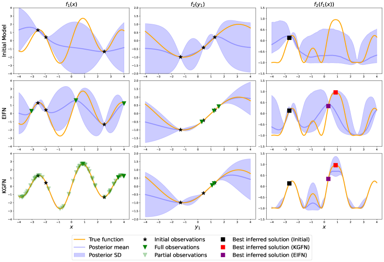
Figure 2: Comparison of EIFN and KGFN on a 1-D synthetic two-stage function network $f_{2}(f_{1}(\cdot))$. The top row, from left to right, shows the initial models for $f_{1}(\cdot)$, $f_{2}(\cdot)$ and $f_{2}(f_{1}(\cdot))$. Similarly, the second and third rows show the resulting models upon budget depletion by EIFN and KGFN. Each true function is represented by an orange curve, while blue curves and shaded blue areas denote posterior mean functions and posterior uncertainty, respectively. Black stars indicate the initial three points fully evaluated across the network for both algorithms. Dark green triangles represent the locations of full network evaluations. Light green triangles represent partial observations where only the first node was evaluated by KGFN. Black, purple and red squares correspond to the initial and two final best inferred solutions identified by EIFN and KGFN, respectively.

3.1 Advantages of Partial Evaluations

In this section, we illustrate the benefits of performing partial evaluations, as permitted by KGFN, through a simple example of a two-stage function. Consider $f_{1}(x)=\sin(x)+2\sin(2x)$ with domain $x\in[-4,4]$, and $f_{2}(y)=\sin(3(y-1)/4)$, which takes as input the output of $f_{1}$. Further, suppose evaluation costs are constant at $c_{1}=1$ for the first stage and $c_{2}=50$ for the second stage. We analyze the behaviors of two acquisition functions: expected improvement of function networks (EIFN), which leverages the network structure and requires full evaluations in each iteration, and KGFN from (2) which allows for partial evaluations and makes decisions in a cost-aware manner.

As shown in Figure 2, both EIFN and KGFN begin with three initial observations (black stars), evaluated across the full network. The initial models for $f_{1}(\cdot)$, $f_{2}(\cdot)$ and $f_{2}(f_{1}(\cdot))$ are presented in the first row of Figure 2. Both algorithms are allocated an evaluation budget of 153, equivalent to performing three full network evaluations. The second and third rows show the evaluations and resulting models upon budget depletion, using EIFN and KGFN, respectively. We find that EIFN makes decisions towards to the goal of identifying the global maximum using the composite network model (third column) without realizing that the first function node is more complicated and its evaluation is more cost-effective. Therefore, EIFN first chooses to evaluate in a region close to the initial best inferred point (black square) and then performs two full evaluations, exploring areas with high uncertainty, such as the boundary at $x=4$, and its best inferred point upon budget depletion (purple square).

In comparison, KGFN takes evaluation costs into account and allocates the budget more efficiently. It first inquires information about the first function node through multiple evaluations (light green triangles) and then evaluates the second node only at the points that it believes will maximize the goal of improving the expected solution quality. This behavior yields a more efficient sampling policy which, in turn, results in a more accurate composite function model and a better best inferred solution (red square).

4 Maximization of KGFN

For simplicity, for the remainder of this paper, we consider cases where $f_{1},\ldots,f_{K}$ are single-output functions.. To solve (3), a natural approach would be to iterate over the set of nodes $\mathcal{V}=\{1,\ldots,K\}$ and individually solve

$$z_{k}^{*}\in\operatorname*{arg\,max}_{z_{k}\in\mathbb{Z}_{k}}\alpha_{n,k}(z_{k}).$$ (4)

Recall that $z_{k}$ consists of $y_{J(k)}\in\mathbb{Y}_{J(k)}$, a combination of outputs from its parent nodes and $x_{I(k)}\in\mathbb{X}_{k}$, some components of the design point $x$. Here, $\mathbb{Y}_{J(k)}$ is a discrete set of combinations of parent nodes’ outputs that have been previously attained. Therefore at each node $k$, the number of KGFN optimization problems (4) is equal to the number of output combinations, which can be huge for complex networks. In addition, another challenge in solving (4) is nested expectations: the outer expectation is with respect to the random variable $f_{k}(z_{k})$ and the inner one is the expectation of the final node value given $\mathcal{D}_{n}$ and $f_{k}(z_{k})$, i.e., $\nu_{n+1}(\cdot)$. In this section, we describe how to compute an approximate solution to (4).

To achieve this goal, we utilize a method called sample average approximation (SAA) (Kim et al.,, 2015). This approach hinges on Monte Carlo (MC) estimates of $\alpha_{n,k}(z_{k})$ in (2), which are deterministic given a set of finite number of random variables independent of $z_{k}$, to provide a differentiable approximation to the acquisition function. This is similar to the approach adopted by Astudillo and Frazier, 2021a . We further relax and thus speed up this estimation through discretization of the design space, optimizing this approximation instead of directly maximizing $\alpha_{n,k}(z_{k})$.

4.1 Monte Carlo Estimation of KGFN

We articulate our method for estimating the value of the KGFN acquisition involving nested expectations.

Understanding that the KGFN acquisition function takes the expectation over the observation $y_{k}=f_{k}(z_{k})$ that results from observing a node $k$ at inputs $z_{k}$, we first use the reparametrization trick (Kingma and Welling,, 2013) to generate samples from the distribution of $f_{k}(z_{k})$. Following Balandat et al., (2020), we call these fantasy samples. We generate $I$ independent standard normal random variables $U^{(i)}$, $i=1,\ldots,I$ and let

$$\hat{y}^{(i)}_{k}=\mu_{n,k}(z_{k})+\sigma_{n,k}(z_{k})U^{(i)}$$

denote these fantasy samples, where $\mu_{n,k}(\cdot)$ and $\sigma_{n,k}(\cdot)$ are the mean and standard deviation of the GP for node $k$ after having observed $n$ samples. Throughout this section, we take the perspective that $n$ samples have already been observed and we are deciding how to allocate sample $n+1$.

Each fantasy sample, if actually observed, would generate a new posterior distribution. Let $\nu_{n+1}^{(i)}(x;z_{k})$ be this new posterior mean of the objective function value at $x$, conditioned on having observed $\hat{y}^{(i)}_{k}$ (we discuss its computation in the next section). Then, an unbiased approximation to the KGFN acquisition is

$$\left[\frac{1}{I}\sum_{i=1}^{I}\max_{x}\nu_{n+1}^{(i)}(x;z_{k})-\nu_{n}^{*}\right]/\,c_{k}(z_{k}).$$

4.2 Estimation of the Posterior Mean

We now describe computation of the posterior mean, $\nu_{n+1}^{(i)}(x;z_{k})$. To explain our approach, we first describe how to generate a sample of the objective function value $y_{K}(x)$ under a particular posterior distribution. This approach is general but we describe it specifically for the posterior that defines $\nu_{n+1}^{(i)}(x;z_{k})$. This is the posterior that conditions on $n$ previous samples and a new observation $\hat{y}^{(i)}_{k}$ of $f_{k}$ at $z_{k}$, which we refer to as the fantasy-$i$ posterior.

We first generate a standard normal random vector $W^{(j)}=(W_{1}^{(j)},W_{2}^{(j)},\ldots,W_{K}^{(j)})^{T}\sim\mathcal{N}(0,I_{K})$ for a single $j$. We include the integer index $j$ because later we will repeat this for several such samples. Then, we recursively define, over all $\ell=1,\ldots,K$, for a generic input $x$ and the proposed point to sample $z_{k}$,

$$\begin{split}\hat{z}^{(i,j)}_{\ell}(x;z_{k})&:=(\hat{y}^{(i,j)}_{J(\ell)}(x;z_{k}),x_{I(\ell)})\\ \hat{y}^{(i,j)}_{\ell}(x;z_{k})&=\mu_{n+1,\ell}^{(i)}(\hat{z}^{(i,j)}_{\ell}(x;z_{k}))\\ &+\sigma_{n+1,\ell}^{(i)}(\hat{z}^{(i,j)}_{\ell}(x;z_{k}))W_{\ell}^{(j)},\end{split}$$ (5)

where $\mu_{n+1,\ell}^{(i)}(\cdot)$ and $\sigma_{n+1,\ell}^{(i)}(\cdot)$ are the mean and standard deviation of the GP for node $\ell$ under the fantasy-$i$ posterior. We use the notation $\hat{y}^{(i,j)}_{\ell}(\cdot;z_{k})$ and $\hat{z}^{(i,j)}_{\ell}(\cdot;z_{k})$ to indicate dependence on $U^{(i)}$, $W^{(j)}$ and the proposed point to measure $z_{k}$.

Given $x$, we can approximate its final node value’s posterior mean $\nu_{n+1}^{(i)}(x;z_{k})$ by drawing many samples independently from a $K$-dimensional standard Gaussian distribution and averaging the resulting final node value samples obtained via (5). For $J$ samples, this estimate is $\frac{1}{J}\sum_{j=1}^{J}\hat{y}^{(i,j)}_{K}\left(x;z_{k}\right)$.

4.3 Putting the Pieces Together

We can now write the following MC estimator for the KGFN acquisition function:

$$\hat{\alpha}_{n,k}(z_{k})=\frac{\frac{1}{I}\sum_{i=1}^{I}\max\limits_{x\in\mathbb{X}}\frac{1}{J}\sum_{j=1}^{J}\hat{y}^{(i,j)}_{K}\left(x;z_{k}\right)-\nu^{*}_{n}}{c_{k}(z_{k})}.$$ (6)

The samples $W^{(j)}$ that drive this MC approximation are shared across all $x$ rather than generated independently. This method of common random variables reduces variance in the MC estimator of KGFN.

To speed up computation of $\hat{\alpha}_{n,k}(z_{k})$, we discretize the set over which we take the maximum for each fantasy-$i$ model in (6) (detailed in Section 4.4). Alternatively, it is possible to replicate the $x$ variable for each index $i$, creating a collection of $x^{(i)}$ variables and then maximize

$$\frac{1}{IJ}\sum_{i=1}^{I}\sum_{j=1}^{J}\hat{y}^{(i,j)}_{K}\left(x^{(i)};z_{k}\right)-\nu^{*}_{n}$$ (7)

jointly over $z_{k}$ and $x^{(i)}$’s in a one-shot fashion similar to Balandat et al., (2020). However, this approach results in an optimization problem where the dimension grows linearly in $I$. This results in an substantial increase in computational time when optimizing the one-shot acquisition. In Appendix B, we compare one-shot optimization and the optimization-via-discretization approach we propose below in terms of computational time and solution quality.

4.4 Optimizing KGFN via Discretization

Following the heuristic initialization method for one-shot optimization in Daulton et al., (2023), we assume that having a single additional observation would not significantly shift the location of the posterior mean maximizer of the updated model from its previous location $x^{*}_{n}$, which can be readily obtained by solving (1). Building on this assumption, to speed up KGFN optimization, we incorporate a discretization method inspired by Frazier et al., (2009); Ungredda et al., (2022) in the algorithm. Specifically, we discretize the domain of maximization problem for $x$ in (6) from the network domain $\mathbb{X}$ to some discrete set of potential candidate solutions $\mathbb{A}$.

Constructing the discrete set $\mathbb{A}$ can be done through several heuristic approaches. Here, we construct $\mathbb{A}$ by taking into account two goals: firstly, exploring the whole domain, and secondly, exploiting the location of the current $x^{*}_{n}$ based on the assumption made above. Hence, in each iteration, we form $\mathbb{A}$ by (i) sampling $N_{R}$ points uniformly across the entire domain $\mathbb{X}$, and (ii) randomly generating $N_{L}$ local points around $x^{*}_{n}$. We define a local point $x\in\mathbb{X}$ to be the ones whose distance $d(x,x^{*}_{n})\leq r||x^{*}_{n}||_{2},$ for some positive parameter $r>0.$ We also include the point $x_{n}^{*}$ itself to $\mathbb{A}$. Therefore, we further approximate $\hat{\alpha}_{n,k}(z_{k})$ in (6) by replacing the domain of the inner maximization by $\mathbb{A}$.

We maximize $\hat{\alpha}_{n,k}(z_{k})$ by enumerating all available (previously evaluated) $y_{J(k)}(x)$ and maximize the acquisition function over $I(k)$ input parameters for each $y_{J(k)}(x)$ using gradients with respect to $I(k)$, which we compute using auto-differentiation. Since $\hat{\alpha}_{n,k}(z_{k})$ is deterministic, we use determinsitic gradient based methods, which has been shown to be fast and effective acquisition optimizers (Daulton et al.,, 2020).

5 Numerical Experiments

We compare the performance of KGFN against several benchmarks, including a random sampling baseline (Random), a standard version of expected improvement (EI), expected improvement for function networks (EIFN), and Thompson sampling for function networks (TSFN). TSFN represents a simple acquisition function leveraging network structures constructed by a series of GP realizations sampled from posterior distributions. All algorithms were implemented in BoTorch (Balandat et al.,, 2020).

We assess performance on several function network structures, including single sequential networks, a multi-process network and a multi-output network. Specifically, we explore two synthetic functions inspired by typical networks in materials design and manufacturing operations, as well as two real-world applications.

In all experiments, each algorithm begins with $2d+1$ points chosen at random over the input space $\mathbb{X}\subseteq\mathbb{R}^{d}$. Each point $x\in\mathbb{X}$ is fully evaluated across the entire network (i.e., we observe $y_{k}(x)$ for $k=1,\cdots,K$). Then, at each iteration, each algorithm sequentially selects a point to evaluate. All four baselines choose a point $x\in\mathbb{X}$ and evaluate the entire network. In contrast, KGFN can take advantage of partial evaluations by selecting both a node $k$ and its input $z_{k}\in\mathbb{Z}_{k}$ to evaluate at each iteration.

We compare performance based on the inference regret $\max_{x}y_{K}(x)-y_{K}(x^{*}_{n})$. Plots show $y_{K}(x^{*}_{n})$, which is the value of the global optimum, $\max_{x}y_{K}(x)$, minus the inference regret. Averaging over 30 replications, we report the means of this metric and $\pm 2$ standard errors over budget used.

5.1 Synthetic Test Problems

(a)

(b)

(c)

Figure 3: Function network structures explored in the numerical experiments: (a) Ackley and FreeSolv, (b) Manu-GP, and (c) Pharm.

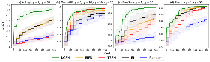
Figure 4: Optimization performance comparing between our proposed KGFN algorithm and benchmarks including EIFN, TSFN, EI and Random on four experiments: (a) Ackley, (b) Manu-GP, (c) FreeSolv, and (d) Pharm.

Ackley6D (Ackley)

We design this problem as a two-stage function network (Figure 3(a)), where the first stage takes a 6-dimensional input and the second stage takes as an input the output of the first stage. The function $f_{1}$ in the first node is the negated Ackley function (Jamil and Yang,, 2013) and the function in the second node is $f_{2}(y_{1})=-y_{1}\times\sin(\frac{5y_{1}}{6\pi})$. This network structure is commonly found in materials design, sequential operations and multi-fidelity settings. In many applications, the early stages in a path through the function network are cheaper-to-evaluate than subsequent stages. For example, the first node can be approximation or partial evaluation of a subsequent node. Therefore, we assume that the costs of evaluations have an ascending order, with $c_{1}=1$ and $c_{2}=50$.

Manufacturing Network (Manu-GP)

Motivated by the manufacturing application from Figure 1, we construct a two-process network where the outputs of the two processes are combined at a final node (Figure 3(b)). The first process has two sequential nodes and its initial input is 2-dimensional. The second process has one node which takes a different 2-dimensional input. This network structure is typical in scenarios where individual components are produced through independent processes and combined to create a final product (e.g., chemical synthesis processes). In this experiment, we employ a sample path drawn from a GP prior for each function node. This is intended to emulate the variations in the characteristics of intermediate/final products, with respect to different design parameters. Since different processes typically have different levels of complexities resulting in heterogeneous costs, here we assume that in the first process $c_{1}=5$ and $c_{2}=10$, and in the second process $c_{3}=10$. Considering that the final stage usually involves both component assembly and product quality assessment, we assume the final stage incurs a relatively high cost, $c_{4}=25$.

5.2 Real-World Applications

Molecular design (FreeSolv)

We utilize the FreeSolv dataset (Mobley and Guthrie,, 2014), which consists of calculated and experimental hydration-free energies of 642 small molecules. A continuous representation is derived from the SMILES representation of each molecule through a variational autoencoder model (Gómez-Bombarelli et al.,, 2018). We apply principal component analysis (PCA) to reduce the dimension of representations to three. In the context of materials design, our objective is to minimize the experimental free energy. Hence, we formulate this problem as a two-stage function network (Figure 3(a)) where the first node takes the 3-dimensional representation of molecules as input and returns the negative calculated free energy. The second node takes the negative calculated free energy as input and returns the negative experimental free energy (our target for maximization). Instead of optimizing over a finite set of candidates, we fit GP surrogate models for both of the two functions based on the entire available dataset. Similar to the Ackley problem, we assume $c_{1}=1$ and $c_{2}=50$.

Pharmaceutical Product Development (Pharm)

An orally disintegrating tablet (ODT) is a drug dosage form designed to dissolve on the tongue. To ensure the production of high-quality ODTs, we must consider two crucial properties: disintegration time $(f_{1})$ and tensile strength ($f_{2}$). We employ surrogate models proposed in Sano et al., (2020) for these two target properties as functions of four input variables in the production process. In the same study, a simple deterministic score function $(f_{3})$, which combines these two targets, is proposed to measure the ODT quality (Figure 3(c)). Here, our goal is to find a set of values for the four input variables that maximizes the score function $f_{3}$. While both target properties are equally significant in determining the quality of the ODT, their measurements typically involve varying levels of complexity. To mirror this, we set $c_{1}=1$ and $c_{2}=50$. Furthermore, the $f_{3}$ score function is known and its evaluation is cost-free. Therefore, it is not included as a node in the KGFN optimization process. Even though $f_{1}$ and $f_{2}$ have overlapping inputs $x$, violating Condition 3, KGFN is still capable of solving this problem as $f_{3}$ is not included in the optimization.

5.3 Results and Discussion

Figure 4 illustrates the performance of KGFN compared to benchmark algorithms in various experiments. Due to requiring full evaluations of function networks, all benchmark algorithms exhibit ladder shapes in their performance curves. KGFN outperforms all benchmarks across all experiments.

In the FreeSolv and Ackley experiments, we observe a behavior similar to the toy example discussed in Section 3.1, where KGFN intelligently allocates the budget to learn the first function node before deciding to explore the second node, and only in regions with high potential values. To examine the impact of evaluation cost on performance, we conduct a sensitivity analysis, varying the evaluation cost of the second in the FreeSolv problem (detailed in Appendix D). When the evaluation costs of the two nodes are equal, KGFN tends to execute full evaluations and achieves performance comparable to the benchmark algorithms. The benefits of partial evaluations become more substantial when the evaluation cost of the second node becomes higher.

Comparing the results across different test problems, we observe that KGFN shows more outstanding performance when downstream nodes in the function network exhibit strong correlations with their parent nodes (Ackley and FreeSolv) and involve higher evaluation costs. This is often the case in real world applications. For example, computer simulators are often engineered to predict the behavior of real-world systems they model while being more cost-effective because they do not require additional resources such as actual materials and trained personnel. In addition, despite the simple networks explored in the numerical experiments, they demonstrate KGFN’s capacity to handle a diverse range of network structures, including sequential networks, multi-process networks and multi-output networks with known objectives.

6 Conclusion

We consider optimizing objectives represented by a network of functions, where individual nodes can be evaluated separately. We develop a new BO acquisition function, KGFN, that makes intelligent decisions about which nodes to evaluate. Our numerical experiments on both synthetic and real-world problems demonstrate that our approach can significantly reduce budget expenditure and provide higher-quality solutions.

While our approach offers substantial advantages through partial evaluations, it has several limitations. First, optimizing KGFN consumes substantial computational resources as it considers all nodes and available outputs at each iteration, which could be challenging for larger networks. However, in many real-world applications where node evaluations are costly and time-consuming, an improved query strategy can outweigh the added computation time, ultimately reducing budget expenditure. Additionally, the opportunity exists to extend and integrate the stock reduction technique presented in Kusakawa et al., (2022), designed for cascade-type networks, to a broader range of network structures to reduce the number of optimization problems considered in KGFN. We leave this as a direction for future work.

Second, our approach is not directly applicable to networks with overlapping inputs. However, one could potentially adapt a network to the framework by reconstructing the network to group nodes that share the same inputs, at the potential loss of some network structure.

Last, our algorithm, like many other KG-based acquisition functions, looks only a single step ahead. An interesting future research direction would be to explore multi-step lookahead acquisition functions for function networks, though this would further increase computational complexity.

Acknowledgments

We thank Eytan Bakshy for their valuable feedback. PB would like to thank DPST scholarship project granted by IPST, Ministry of Education, Thailand for providing financial support. PF was supported by AFOSR FA9550-19-1-0283 and FA9550-20-1-0351.

Supplementary Materials for
Bayesian Optimization of Function Networks With
Partial Evaluations

Appendix A Pseudo-Code for the KGFN Algorithm

We present the pseudo-code for implementing Bayesian optimization with the KGFN acquisition function, supplementing the descriptions in Section 4. Algorithm 1 outlines the BO loop employing the KGFN algorithm. Algorithm 2 describes the computation of the MC estimate of the acquisition value. Algorithm 3 describes how we estimate the posterior mean of the final function node via MC simulation, which is necessary for Algroithm 2. We defer the discussion of acquisition optimization to Appendix B, where we compare our implementation, optimization-via-discretization, against a commonly used approach, one-shot optimization.

Algorithm 1 Bayesian Optimization using KGFN

input:
      $c_{k}(\cdot)$, the evaluation cost function for node $k$, $k=1,\ldots,K$
      $B$, the total evaluation budget
      $\mu_{0,k}(\cdot)$ and $\sigma_{0,k}(\cdot)$, the mean and standard deviation of the GP for node $k$, $k=1,\ldots,K$ (fitted using initial observations)
output: the point with the largest posterior mean at the final function node

1:$n\leftarrow 0$

2:$b\leftarrow 0$

3:while $b<B$ do

4:     $n\leftarrow n+1$

5:     for $k=1,\ldots,K$ do

6:         identify the set of combinations of previously evaluated $y_{J(k)}(x)$, $\mathbb{Y}_{J(k)}$

7:         if $\mathbb{Y}_{J(k)}=\emptyset$ then

8:              $\hat{\alpha}_{n,k}^{*}\leftarrow-1$

9:         else

10:              $\hat{\alpha}_{n,k}^{*}\leftarrow\max_{z\in\mathbb{Y}_{J(k)}\times\mathbb{X}_{I(k)}}\hat{\alpha}_{n,k}(z)$ where $\hat{\alpha}_{n,k}(\cdot)$ is computed using Algorithm 2

11:              $z_{k}^{*}\leftarrow\operatorname*{arg\,max}_{z\in\mathbb{Y}_{J(k)}\times\mathbb{X}_{I(k)}}\hat{\alpha}_{n,k}(z)$

12:              if $c_{k}(z_{k}^{*})>B-b$ then

13:                  $\hat{\alpha}_{n,k}^{*}\leftarrow-1$

14:              end if

15:         end if

16:     end for

17:     if $\max_{k}\hat{\alpha}_{n,k}^{*}=-1$ then

18:         break

19:     else

20:         $k^{*}\leftarrow\operatorname*{arg\,max}_{k\in\{1,\ldots,K\}}\hat{\alpha}_{n,k}^{*}$

21:         obtain $y_{k^{*}}=f_{k^{*}}(z^{*}_{k^{*}})$

22:         update the GP model for node $k^{*}$ with the additional observation $(z^{*}_{k^{*}},y_{k^{*}})$

23:         $b\leftarrow b+c_{k^{*}}(z_{k^{*}}^{*})$

24:     end if

25:end while

return $\operatorname*{arg\,max}_{x\in\mathbb{X}}\hat{\nu}_{n}(x)$, an estimate of $\nu_{n}(x)$ given in Algorithm 3 using a gradient-based method

Algorithm 2 MC Estimate of $\alpha_{n,k}(z_{k})$

input:
      $k$, the node to be evaluated
      $z_{k}$, the input for node $k$
      $c_{k}(\cdot)$, the evaluation cost function for node $k$
      $I$, the number of fantasy observations to create
      $J$, the number of MC samples for estimating the posterior mean of the final function node
      $\mu_{n,\ell}(\cdot)$ and $\sigma_{n,\ell}(\cdot)$, the mean and standard deviation of the GP for node $\ell$, $\ell=1,\ldots,K$
output: $\hat{\alpha}_{k,n}(z_{k})$, the estimated acquisition value

1:solve $\max_{x\in\mathbb{X}}\hat{\nu}_{n}(x)$, an estimate of $\nu_{n}(x)$ given in Algorithm 3 using a gradient-based method and obtain $\hat{\nu}_{n}^{*}$

2:generate $I$ independent standard normal random variables $U^{(i)}$, $i=1,\ldots,I$

3:for $i=1,\ldots,I$ do

4:     $\hat{y}_{k}^{(i)}\leftarrow\mu_{n,k}(z_{k})+\sigma_{n,k}(z_{k}){U}^{(i)}$

5:     update the posterior of GP for node $k$ with the additional observation $\left(z_{k},\hat{y}_{k}^{(i)}\right)$

6:     solve $\max_{x\in\mathbb{X}}\hat{\nu}^{(i)}_{n+1}(x)$ to obtain $\hat{\nu}_{n+1}^{(i)*}$ for fantasy-$i$ model using Algorithm 3

7:end for

8:$\hat{\alpha}_{k,n}(z_{k})\leftarrow\frac{1}{c_{k}(z_{k})}\left(\frac{1}{I}\sum_{i=1}^{I}\hat{\nu}^{(i)*}_{n+1}-\hat{\nu}_{n}^{*}\right)$

9:return $\hat{\alpha}_{k,n}(z_{k})$

Algorithm 3 Posterior Mean Estimate of the Final Function Node via MC Simulation

input:
      $x\in\mathbb{X}$, a design point of the function network
      $J$, the number of MC samples
      $\mu_{\ell}(\cdot)$ and $\sigma_{\ell}(\cdot)$, the mean and standard deviation of the GP for node $\ell$, for $\ell=1,\ldots,K$
output: $\hat{\nu}(x)$, the estimated posterior mean

1:generate $J$ independent samples $W^{(j)}=\left(W_{1}^{(j)},W_{2}^{(j)},\ldots,W_{K}^{(j)}\right)^{T}$ for $j=1,\ldots,J$ from $\mathcal{N}(0,I_{K})$;

2:for $j=1,\ldots,J$ do

3:     for $\ell=1,\ldots,K$ do

4:         define $\hat{z}^{(j)}_{\ell}(x):=(\hat{y}^{(j)}_{J(\ell)}(x),x_{I(\ell)})$

5:         $\hat{y}^{(j)}_{\ell}(x)\leftarrow\mu_{\ell}(\hat{z}^{(j)}_{\ell}(x))+\sigma_{\ell}(\hat{z}^{(j)}_{\ell}(x))W_{\ell}^{(j)}$

6:     end for

7:end for

8:$\hat{\nu}(x)\leftarrow\frac{1}{J}\sum_{j=1}^{J}\hat{y}^{(j)}_{K}(x)$

9:return $\hat{\nu}(x)$

Appendix B Additional Details on Acquisition Function Optimization

We describe model configuration and hyperparameters used to optimize the acquisition functions used in our numerical experiments. Moreover, we present a comparison between the one-shot optimization and optimization-via-discretization approaches for optimizing the KGFN acquisition.

B.1 Hyperparameters in Acquisition Function Optimization

In our experiments, all methods utilize independent GPs with zero mean functions and the Mateŕn 5/2 kernel genton2001classes, with automatic relevance determination (ARD). The lengthscales of the GPs are assumed to have Gamma priors: for the Ackley, FreeSolv and Pharm problems, Gamma(3, 6); for the Manu-GP problem, Gamma(5, 2). The outputscale parameters are assumed to have Gamma(2, 0.15) priors in all problems. The lengthscales and outputscales are then estimated via maximum a posteriori (MAP) estimation.

In KGFN, we estimate the posterior mean of a function network’s final node value with $J=64$ quasi-MC samples using Sobol sequences balandat2020botorch. For EIFN, we follow the implementation in astudillo2021bayesian, using $J=128$.

To provide MC estimates for the KGFN acquisition value, we use $I=8$ fantasy models. As described in Section 4.4, we optimize the KGFN acquisition function via discretization, replacing the domain of the optimization problem in line 6 of Algorithm 2 by a discrete set of candidate solutions $\mathbb{A}$. We include in $\mathbb{A}$ the current maximizer of the final node posterior mean $x_{n}^{*}$, $N_{R}=10$ points selected randomly from the domain $\mathbb{X}$, $N_{L}=10$ local points satisfying $d(x,x_{n}^{*})\leq r\|x^{*}_{n}\|_{2}$ where $r=0.2$.

When optimizing EIFN, TSFN, or KGFN for a problem with $d$-dimensional function network input, we use $100d$ raw samples for initialization and $10d$ starting points for multi-start optimization. We set the number of initializations to 100 and the number of restarts to 20 when optimizing the standard EI acquisition function.

All algorithms are implemented in the open source BoTorch package balandat2020botorch. We extend the implementation outlined in astudillo2021bayesian to enable partial evaluations for function networks.

B.2 Comparison Between One-Shot Optimization and Optimization-Via-Discretization

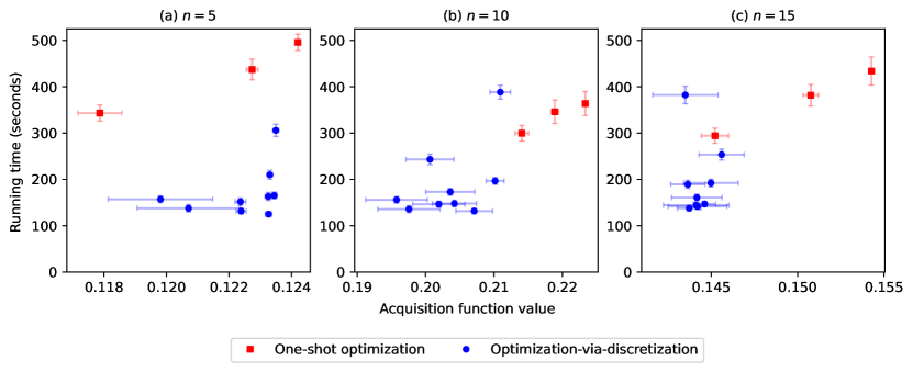
Figure B.1: Comparison between one-shot optimization and optimization-via-discretization in terms of acquisition value attained and computational time, on the Ackley6D problem with different numbers of fully-evaluated points: (a) $n=5$, (b) $n=10$, and (c) $n=15$. Both the value averaging over 100 trials and the standard error are presented.

We perform a comparison analysis between two popular methods for optimizing KG-based acquisition functions, one-shot optimization and optimization-via-discretization.

The one-shot optimization method, proposed by Balandat et al., (2020), has gained popularity in optimizing non-myopic acquisition functions in recent years jiang2020efficient, astudillo2021multi, daulton2023hvkg. This method effectively addresses the nested optimization problem, a common challenge encountered when optimizing KG. However, it introduces its own challenges – namely, by turning the nested optimization problem into a single high-dimensional (and typically more difficult) optimization problem, the one-shot optimization approach can be more likely to get stuck in local optima and result in high computational time (due to the higher number of optimization variables, and the potential of the numerical optimization failing to converge).

Optimization-via-discretization, first introduced in frazier2009knowledge, is a commonly used alternative technique for optimizing KG ungredda2022efficient, buckingham2023bayesian. This method accelerates KG optimization by discretizing the domain of the inner optimization problem. Nevertheless, it has its own limitation, as the discretization will lead to less accurate solution for the inner optimization problem, potentially resulting in sub-optimal outcomes, especially in higher dimensions (due to the coarser coverage of the space).

Our method follows the optimization-via-discretization approach. However, rather than selecting points randomly within the domain or arranging them in a grid, we intelligent choose the points that form the discrete set for the inner optimization problem (see Section 4.4).

To better understand the performance of one-shot optimization and optimization-via-discretization in the context of optimizing KGFN, we conduct a comparison analysis. Specifically, we examine both approaches under different configurations using the Ackley6D test problem. We consider problem instances where we have access to 5, 10, and 15 full evaluations of the function network. These observations are held fixed and used to fit GP network models. We seek to optimize KGFN at the first function node.

For both approaches, we explore three choices for the number of fantasy models, $I=2,4$, and 8, for estimating the KGFN acquisition values. In the optimization-via-discretization approach, we consider three discrete set sizes for the inner optimization problem: $|\mathbb{A}|=11$ ($N_{R}=N_{L}=5$), $|\mathbb{A}|=21$ ($N_{R}=N_{L}=10$), and $|\mathbb{A}|=41$ ($N_{R}=N_{L}=20$). We measure performance in terms of both true acquisition function value of the selected candidates (approximated by the MC estimator described in Algorithm 2, with $I=512$ and $J=128$) and computational time (measured in seconds), averaging over 100 trials.

We observe that although one-shot optimization demonstrates the best performance in terms of acquisition value attained, optimization-via-discretization can attain comparable acquisition value with significantly reduced running time (see Figure B.1). For the setup used in our experiments ($I=8$ and $|\mathbb{A}|=21$), optimization-via-discretization achieves slightly lower acquisition value compared to the best-performing one-shot optimization method with $I=8$ (0.60%, 5.9%, and 6.02% lower for the problem instances with 5, 10, and 15 fully evaluated points, respectively). However, it significantly reduces the average running time compared to the best-performing one-shot optimization algorithm, by 66.7%, 45.9%, and 55.8%. The significant reduction in running time, along with the marginal loss in acquisition values, justifies the employment of the discretization approach in our experiments. The full comparison analysis results are summarized in Table B.1.

Table B.1: Comparisons between one-shot optimization and optimization-via-discretization on the Ackley6D test problem, with 5, 10, and 15 design points fully evaluated across the network. Performances are reported in terms of acquisition function value obtained and running time. Both the value averaging over 100 trials and the standard error are reported. Numbers in boldface denote the highest acquisition function value and the shortest running time.

(a) Number of fully evaluated points: 5
Method	Num of fantasy models $I$	Size of discrete set $|\mathbb{A}|$	Avg. acqf. val.	Avg. running time (seconds)
One-shot	2	NA	$0.11787\pm 0.00070$	$343\pm 17$
	4	NA	$0.12274\pm 0.00019$	$437\pm 22$
	8	NA	$\mathbf{0.12420\pm 0.00004}$	$496\pm 18$
Discretization	2	11	$0.12239\pm 0.00016$	$\mathbf{132\pm 6\;}$
	2	21	$0.11236\pm 0.00017$	$151\pm 8\;$
	2	41	$0.11981\pm 0.00167$	$157\pm 8\;$
	4	11	$0.12070\pm 0.00164$	$138\pm 8\;$
	4	21	$0.12325\pm 0.00010$	$163\pm 9\;$
	4	41	$0.12330\pm 0.00009$	$210\pm 10$
	8	11	$0.12326\pm 0.00011$	$125\pm 6\;$
	8	21	$0.12345\pm 0.00009$	$165\pm 7\;$
	8	41	$0.12350\pm 0.00009$	$306\pm 13$
(b) Number of fully evaluated points: 10
Method	Num of fantasy models $I$	Size of discrete set $|\mathbb{A}|$	Avg. acqf. val.	Avg. running time (seconds)
One-shot	2	NA	$0.2141\pm 0.0010$	$300\pm 17$
	4	NA	$0.2190\pm 0.0005$	$346\pm 25$
	8	NA	$\mathbf{0.2234\pm 0.0002}$	$364\pm 26$
Discretization	2	11	$0.2071\pm 0.0027$	$\mathbf{132\pm 6\;}$
	2	21	$0.2019\pm 0.0038$	$147\pm 6\;$
	2	41	$0.2036\pm 0.0036$	$173\pm 7\;$
	4	11	$0.1976\pm 0.0045$	$136\pm 8\;$
	4	21	$0.1958\pm 0.0045$	$156\pm 7\;$
	4	41	$0.2006\pm 0.0035$	$243\pm 11$
	8	11	$0.2042\pm 0.0032$	$148\pm 7\;$
	8	21	$0.2102\pm 0.0013$	$197\pm 8\;$
	8	41	$0.2109\pm 0.0014$	$388\pm 15$
(c) Number of fully evaluated points: 15
Method	Num of fantasy models $I$	Size of discrete set $|\mathbb{A}|$	Avg. acqf. val.	Avg. running time (seconds)
One-shot	2	NA	$0.1452\pm 0.0008$	$294\pm 16$
	4	NA	$0.1508\pm 0.0005$	$382\pm 23$
	8	NA	$\mathbf{0.1543\pm 0.0001}$	$434\pm 30$
Discretization	2	11	$0.1437\pm 0.0007$	$\mathbf{138\pm 6\;}$
	2	21	$0.1446\pm 0.0006$	$147\pm 6\;$
	2	41	$0.1436\pm 0.0010$	$189\pm 9\;$
	4	11	$0.1442\pm 0.0017$	$142\pm 6\;$
	4	21	$0.1442\pm 0.0015$	$161\pm 7\;$
	4	41	$0.1456\pm 0.0013$	$253\pm 12$
	8	11	$0.1441\pm 0.0020$	$144\pm 5\;$
	8	21	$0.1450\pm 0.0016$	$192\pm 8\;$
	8	41	$0.1435\pm 0.0020$	$382\pm 19$

Appendix C Additional Details on Numerical Experiments

We provide more details on the numerical experiments presented in the main manuscript.

C.1 Ackley6D (Ackley)

We design the Ackley synthetic test problem as a two-stage function network (Figure 3(a)). The first function node is the 6-dimensional negated Ackley function ackley2012connectionist:

$$f_{1}(x)=20\exp\left(-0.2\sqrt{\frac{1}{6}\sum_{i=1}^{6}x_{i}^{2}}\right)+\exp\left(\frac{1}{6}\sum_{i=1}^{6}\cos{(2\pi x_{i})}\right)-20-\exp(1),$$

where $x_{i}\in[-2,2]$ for $i=1,\ldots,6$. The second function node, which takes as an input the output of the first function node, is defined as follows

$$f_{2}(y)=-y\sin{\left(\frac{5y}{6\pi}\right)}.$$

C.2 Manufacturing Network (Manu-GP)

Motivated by real-world manufacturing applications where several intermediate parts are produced and then assembled to create a final product, we formulate this second test problem involving two processes, each of which takes a two-dimensional input (Figure 3(b)). The first process consists of two sequential sub-processes, denoted as $f_{1}$ and $f_{2}$. The first sub-process takes $x_{1},x_{2}$ as inputs and returns $y_{1}$ which is taken by the second sub-process to produce an output $y_{2}$. The second process, $f_{3}$, takes $x_{3}$ and $x_{4}$ as input and produces an output $y_{3}$. The outputs $y_{2}$ and $y_{3}$ are then combined in the final process $f_{4}$ to produce a final output $y_{4}$, which we aim to maximize. This experiment is designed to mimic a manufacturing scenario. Here, we set each input $x_{i}\in[-1,1]$, for $i=1,\ldots,4$.

For each function node, we draw a sample path from a GP prior with the Matérn 5/2 kernel genton2001classes. Notably, we choose different lengthscales in the kernels for difference function nodes: 0.631 for $f_{1}$, 1 for $f_{2}$, 1 for $f_{3}$, and 3 for $f_{4}$. The outputscale parameter in the kernel is set to 0.631 for all functions but $f_{4}$, which has outputscale equal to 10. We show the drawn sample paths for each of the function nodes in Figure C.2.

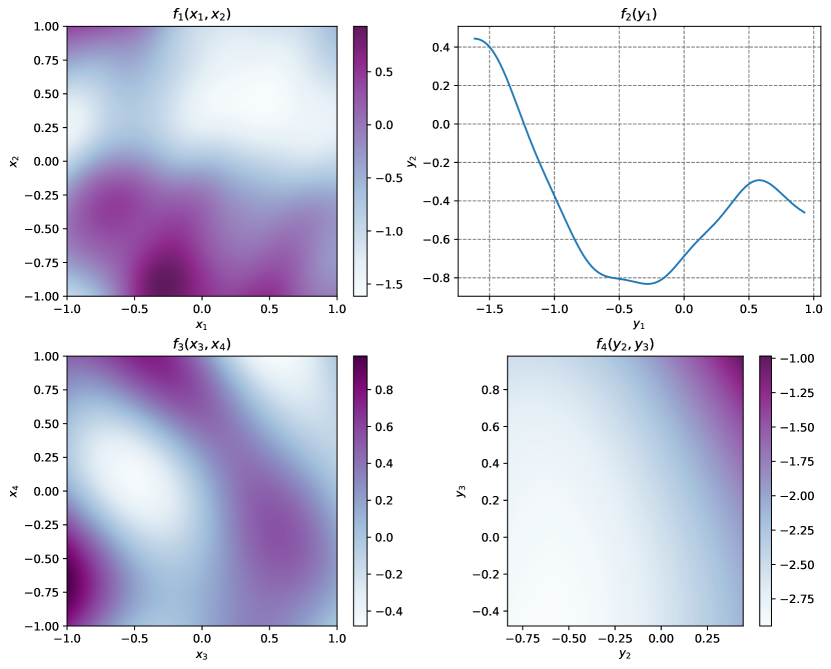
Figure C.2: The sample paths drawn from GP priors for the manufacturing problem.

C.3 Molecular Design (FreeSolv)

We obtain the FreeSolv dataset from mobley2014freesolv, which comprises both calculated and experimental free energies (in kcal/mol) for 642 small molecules. Since lower free energy is preferred, we negate free energy (both calculated and experimental), setting our objective to maximizing the negative experimental free energy.

To represent each small molecule in a continuous space, we utilize a variational autoencoder trained on the Zinc dataset as studied in gomez2018automatic, resulting in a 196-dimensional representation in the unit cube, i.e., $x\in[0,1]^{196}$. We reduce the dimentionality of the representation to three through the standard principal component analysis (PCA) technique.

We then utilize the entire dataset to train two GP models, and use the posterior mean of the trained model as the underlying functions in the function network (Figure 3(a)):

1. $f_{1}$ takes a three-dimensional representation as input and predicts the negative calculated free energy $y_{1}$;

2. $f_{2}$ takes the negative calculated free energy as input and predicts the negative experimental free energy (shown in Figure C.3).

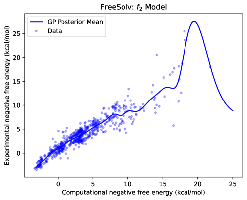
Figure C.3: The posterior mean function of the GP fitted between calculated and experimental free energies.

C.4 Pharmaceutical Product Development (Pharm)

In this test problem, we tackle the challenge of manufacturing orally disintegration tablets (ODTs) that meet pharmaceutical standards, focusing on two crucial properties: disintegration time ($f_{1}$) and tensile strength ($f_{2}$). To model these properties, we adopt the neural network (NN) models proposed in sano2020application.

Specifically, the two properties are defined as functions of four parameters describing the production process, namely, $\beta$ form D-mannitol ratio in the total D-mannitol $(x_{1})$, L-HPC ratio in a formulation $(x_{2})$, granulation fluid level $(x_{3})$ and compression force $(x_{4})$. Each parameter $x_{i}$ is constrained to the range $[-1,1]$. The fitted NN models are shown as follows:

$$f_{1}(x) =-3.95+9.20\times(1+\exp(-(0.32+5.06x_{1}-4.07x_{2}-0.36x_{3}-0.34\times x_{4}))^{-1}$$

$$\qquad+9.88\times(1+\exp(-(-4.83+7.43x_{1}+3.46x_{2}+9.19x_{3}+16.58x_{4})))^{-1}$$

$$\qquad+10.84\times(1+\exp(-7.90-7.91x_{1}-4.48x_{2}-4.08x_{3}-8.28x_{4}))^{-1}$$

$$\qquad+15.18\times(1+\exp(-(9.41-7.99x_{1}+0.65x_{2}+3.14x_{3}+0.31x_{4})))^{-1}.$$

and

$$f_{2}(x) =1.07+0.62\times(1+\exp(-(3.05+0.03x_{1}\textendash 0.16x_{2}+4.03x_{3}-0.54x_{4})))^{-1}$$

$$\qquad+0.65\times(1+\exp(-(1.78+0.60x_{1}-3.19x_{2}+0.10x_{3}+0.54x_{4})))^{-1}$$

$$\qquad-0.72\times(1+\exp(-(0.01+2.04x_{1}-3.73x_{2}+0.10x_{3}-1.05x_{4})))^{-1}$$

$$\qquad-0.45\times(1+\exp(-(1.82+4.78x_{1}+0.48x_{2}-4.68x_{3}-1.65x_{4})))^{-1}$$

$$\qquad-0.32\times(1+\exp(-(2.69+5.99x_{1}+3.87x_{2}+3.10x_{3}-2.17x_{4})))^{-1},$$

To measure the quality of a tablet, the same study introduced a score function $f_{3}$ (treated as a known function in our experiment), which combines the two properties $f_{1}$ and $f_{2}$:

$$f_{3}=\frac{(60-f_{1})}{60}\times\frac{f_{2}}{1.5},$$

where the first term aims to ensure that the disintegration time is not too long (less than 60 seconds), and the second term aims to ensure that the tensile strength is large enough for production and distribution.

Appendix D Sensitivity Analysis for Evaluation Costs

We conduct a sensitivity study to examine the impact of cost functions on the optimization performance across three experiments with two nodes to evaluate: Ackley, FreeSolv and Pharm. In these experiments, we investigate three cost function scenarios: (a) $c_{1}=1,c_{2}=1$; (b) $c_{1}=1,c_{2}=10$; and (c) $c_{1}=1,c_{2}=50$, which correspond to the situations where both nodes have similar evaluation costs, where one node has a higher evaluation cost than the other, and where one node has an exceptionally high evaluation cost, respectively. The evaluation budgets for each problem are set to 50, 150, and 700 in the three scenarios.

The performance curves, shown in Figures D.4, reveal that performing partial evaluations notably improve optimization performance, especially when the costs of the two nodes are dramatically different. On the other hand, in the equal-cost scenario, KGFN takes less advantage of partial evaluating, tending to complete full evaluations in sequential networks (Ackley and FreeSolv), and choose to evaluate the two properties in Pharm problem equal number of times.

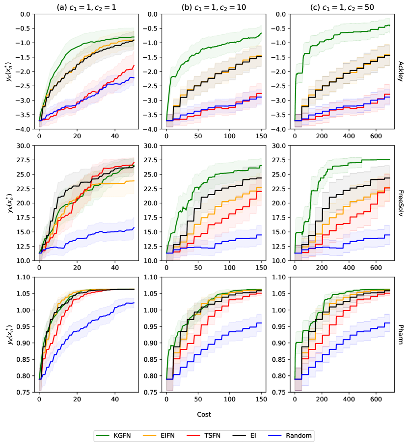
Figure D.4: Cost sensitivity analysis for (from top to bottom) Ackley, FreeSolv and Pharm problems with different costs: (a) $c_{1}=1,c_{2}=1$; (b) $c_{1}=1,c_{2}=10$; and (c) $c_{1}=1,c_{2}=50$. The performance metric is the true objective value at the maximizer of final function node’s posterior mean versus the budget spent.

ref apalike

References

- Alvarez et al., (2012) Alvarez, M. A., Rosasco, L., Lawrence, N. D., et al. (2012). Kernels for vector-valued functions: A review. Foundations and Trends® in Machine Learning, 4(3):195–266.