Sparse Training of Discrete Diffusion Models for Graph Generation

Abstract

Generative models for graphs often encounter scalability challenges due to the inherent need to predict interactions for every node pair. Despite the sparsity often exhibited by real-world graphs, the unpredictable sparsity patterns of their adjacency matrices, stemming from their unordered nature, leads to quadratic computational complexity. In this work, we introduce SparseDiff, a denoising diffusion model for graph generation that is able to exploit sparsity during its training phase. At the core of SparseDiff is a message-passing neural network tailored to predict only a subset of edges during each forward pass. When combined with a sparsity-preserving noise model, this model can efficiently work with edge lists representations of graphs, paving the way for scalability to much larger structures. During the sampling phase, SparseDiff iteratively populates the adjacency matrix from its prior state, ensuring prediction of the full graph while controlling memory utilization. Experimental results show that SparseDiff simultaneously matches state-of-the-art in generation performance on both small and large graphs, highlighting the versatility of our method.

1 Introduction

Random graph models have been foundational in graph generation, with a rich legacy spanning several decades (Erdős et al., 1960; Aiello et al., 2000; Barabási, 2013). However, recent interest has gravitated towards learned graph models, primarily due to their enhanced ability to represent intricate data distributions. Traditional frameworks like generative adversarial networks (De Cao & Kipf, 2018) and variational autoencoders (Simonovsky & Komodakis, 2018) predominantly addressed graphs with a maximum of 9 nodes. This limitation was somewhat alleviated with the advent of denoising diffusion models (Niu et al., 2020; Jo et al., 2022; Vignac et al., 2023a), elevating capacity to roughly 100 nodes. However, these models are still not scaled for broader applications like transportation (Rong et al., 2023) or financial system anomaly detection (Li et al., 2023).

The primary bottleneck of many generative graph models is their computational complexity. While many natural graphs are sparse, the unordered nature graphs makes it challenging to exploit this trait. Without a predetermined sparsity pattern, models frequently make exhaustive predictions for every node pair, constraining them to a ceiling of $\sim$200 nodes (Vignac et al., 2023a). Proposed methods to circumvent this issue include imposing a node ordering (Dai et al., 2020), assembling sub-graphs (Limnios et al., 2023), generating hierarchically (Karami, 2023; Jang et al., 2023), and conditioning the generation on a sampled degree distribution (Chen et al., 2023). These methods, designed for large graphs, implicitly make assumptions on the data distribution which sometimes reflect in a poor ability to model very constrained graphs such as molecules (Chen et al., 2023; Kong et al., 2023).

To address these limitations, we propose SparseDiff, a generative model for graphs that exploits sparsity in its training phase by adopting edge list representations. SparseDiff defines a discrete denoising diffusion model that comprises three primary components:

1. A noise model designed to retain sparsity throughout the diffusion process;

2. A loss function computed on a set of random node pairs;

3. A sparse graph transformer rooted in the message-passing framework.

During the sampling process, our model iterates over pairs of nodes and progressively builds the predicted graph. Setting it apart from other scalable models, SparseDiff harnesses sparsity inherently without imposing additional assumptions on the data distribution. As a result, it also encompasses dense denoising diffusion models as a limit case.

We show across a wide range of benchmarks that despite its simplicity, SparseDiff matches the generation performance of scalable models on large graphs. It also achieves comparable results to state-of-the-art dense models on small molecular datasets, making our model fit for all graph sizes. Overall, SparseDiff provides high controllability over GPU usage and thus extends the capabilities of current discrete graph models, making them suitable for significanlty larger graphs.

(a) Ego training set ($50$ to $399$ nodes).

(b) Generated Ego graphs.

(c) Protein training set ($100$ to $500$ nodes).

(d) Generated Protein graphs.

Figure 1: Samples from SparseDiff trained on large graphs.

2 Related Work

2.1 Denoising diffusion models for graphs

Diffusion models (Sohl-Dickstein et al., 2015; Ho et al., 2020) have gained increasing popularity as generative models due to their impressive performance across generative tasks in computer vision (Dhariwal & Nichol, 2021; Ho et al., 2022; Poole et al., 2022), protein generation (Baek et al., 2021; Ingraham et al., 2022) or audio synthesis (Kong et al., 2020). They can be trained by likelihood maximization (Song et al., 2020; Kingma et al., 2021), which provides stability gains over generative adversarial networks, and admit a stochastic differential equation formulation (Song et al., 2020). Two core components define these models. The first is a Markovian noise model, which iteratively corrupts a data point $x$ to a noisy sample $z^{t}$ until it conforms to a predefined prior distribution. The second component, a denoising network, is trained to revert the corrupted data to a less noisy state. This denoising network typically predicts the original data $x$ or, equivalently, the added noise $\epsilon$.

After the denoising network has been trained, it can be used to sample new objects. First, some noise $z^{T}$ is sampled from a prior distribution. The denoising network is then iteratively applied to this object. At each time step, a distribution $p_{\theta}(z^{t-1}|z^{t})$ is computed by marginalizing over the network prediction $p_{\theta}(x)$:

$$p_{\theta}(z^{t-1}|z^{t})=\int_{x}q(z^{t-1}|z^{t},x)~{}dp_{\theta}(x),$$

and a new object is sampled from this distribution. While this integral is in general difficult to evaluate, two prominent frameworks allow for its efficient computation: Gaussian diffusion (Ho et al., 2020) and discrete diffusion (Austin et al., 2021).

When tailored to graph generation, initial diffusion models employed Gaussian noise on the adjacency matrices (Niu et al., 2020; Jo et al., 2022). They utilized a graph attention network to regress the added noise $\epsilon$. Given that $\epsilon=z^{t}-z$, regressing the noise is, up to an affine transformation, the same as regressing the clean graph, which is a discrete object. Recognizing the inherent discreteness of graphs, subsequent models (Vignac et al., 2023a; Haefeli et al., 2022) leveraged discrete diffusion. They recast graph generation as a series of classification tasks, preserving graph discreteness and achieving top-tier results. However, they made predictions for all pairs of nodes, which restricted their scalability.

2.2 Scalable Graph Generation

Efforts to enhance the scalability of diffusion models for graph generation have mainly followed two paradigms: subgraph aggregation and hierarchical refinement.

Subgraph Aggregation

This approach divides larger graphs into smaller subgraphs, which are subsequently combined. Notably, SnapButton (Yang et al., 2021) enhances autoregressive models (Liu et al., 2018; Liao et al., 2019; Mercado et al., 2021) by merging subgraphs. Meanwhile, BiGG (Dai et al., 2020) deconstructs adjacency matrices using a binary tree data structure, gradually generating edges with an autoregressive model. One notable limitation of autoregressive models is the breaking of permutation equivariance due to node ordering dependency. To counter this, (Kong et al., 2023) proposed learning the node ordering – a task theoretically at least as hard as isomorphism testing. Separately, SaGess (Limnios et al., 2023) trains a dense DiGress model to generate subgraphs sampled from a large graph, and then merges these subgraphs.

Hierarchical Refinement

This class of methods initially generates a rudimentary graph, which undergoes successive refinements for enhanced detail (Yang et al., 2021; Karami, 2023). Illustrative of this approach, the HGGT model (Jang et al., 2023) employs a $K^{2}$-tree representation. Specifically for molecular generation, fragment-based models, such as (Jin et al., 2018; 2020; Maziarz et al., 2022), adeptly assemble compounds using pre-defined molecular fragments.

A unique approach outside these paradigms was presented by Chen et al. (2023), who initially generated a node degree distribution ${\bm{d}}^{0}$ for the nodes, and subsequently crafted an adjacency matrix ${\bm{A}}$ conditioned on this distribution, preserving sparsity. Despite the universal feasibility of this factorization, the ease of learning the conditional distribution $p_{\theta}({\bm{A}}|{\bm{d}}^{0})$ remains incertain, as there does not even always exist undirected graphs that satisfy a given degree distribution.

Overall, scalable generation models typically either introduce a dependence on node orderings, or rely heavily on the existence of a community structure in the graphs. In contrast, the SparseDiff model described in next section aims at making no assumption besides sparsity, which results in very good performance across a wide range of graphs.

3 SparseDiff: Sparse Denoising Diffusion for Large Graph Generation

We introduce the Sparse Denoising Diffusion model (SparseDiff), designed to bolster the scalability of discrete diffusion models by adopting edge list representations of graphs. While our primary focus is on graphs with discrete node and edge attributes, our model can be readily extended to accommodate continuous node attributes as well.

A graph $G$, composed of $n$ nodes and $m$ edges, is denoted as a triplet $({\bm{E}},{\bm{X}},{\bm{Y}})$. Here, ${\bm{E}}\in\mathbb{N}^{2\times m}$ represents the edge list detailing indices of endpoints, while the node and edge attributes are encapsulated using a one-hot format in ${\bm{X}}\in\{0,1\}^{n\times a}$ and ${\bm{Y}}\in\{0,1\}^{m\times b}$, respectively.

The method’s schematic is depicted in Fig. 2. SparseDiff integrates three key components for training using sparse representations: a noise model that preserves sparsity in the graphs, a graph transformer that operates on sparse representations, and a loss function computed on random pairs of nodes. This integration facilitates efficient model training. However, it is crucial to note that during sampling, our model’s complexity remains quadratic in $n$.

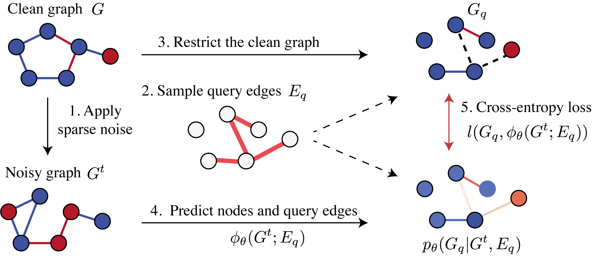
Figure 2: Overview of SparseDiff. In order to train a denoising neural network without considering all pairs of nodes, SparseDiff combines i) a noise model that preserves sparsity during diffusion; ii) a graph transformer $\phi_{\theta}$ implemented within the message-passing framework; iii) a loss function computed on a subset ${\bm{E}}_{q}$ of all pairs of nodes. Together, these components allow for using edge lists and training diffusion models on significantly larger graphs than dense methods.

3.1 Sparsity-preserving noise model

Our framework requires a noise model that preserves the sparsity of edges during diffusion. This rules out Gaussian-based models, and we therefore build our model on the discrete diffusion framework of Austin et al. (2021).

In discrete diffusion, adding noise means jumping from state to state, i.e., sampling a state from a categorical distribution. The transition probabilities are given by a Markov transition matrix ${\bm{Q}}^{t}$ for each time step $t$, where ${\bm{Q}}^{t}[i,j]$ is the probability of transitioning from state $i$ to state $j$ . In the context of graph generation, the states corresponds to the possible node types or edge types, one particular state for the edges being ”no edge”. The noise model is a product over nodes and edges, which means that nodes and edges are corrupted independently. In batch form, the noise model can therefore be written $q(G^{t}|G^{t-1})=({\bm{X}}^{t-1}{\bm{Q}}^{t}_{\bm{X}},{\bm{Y}}^{t-1}{\bm{Q}}^{t}_{{\bm{Y}}})$, where ${\bm{Q}}^{t}_{\bm{X}}$ and ${\bm{Q}}^{t}_{{\bm{Y}}}$ refers to the transition matrix at step $t$ for nodes and edges respectively, while ${\bm{Y}}\in\mathbb{N}^{n\times n\times b}$ contains all edge features in dense format. Since the noise model is markovian, there noise does not need to be added recursively, and $q(G^{t}|G)$ can be obtained by multiplying the Markov transition matrices: $q(G^{t}|G)=({\bm{X}}\bar{\bm{Q}}^{t}_{\bm{X}},{\bm{Y}}\bar{\bm{Q}}^{t}_{{\bm{Y}}})$, with $\bar{{\bm{Q}}}^{t}={\bm{Q}}^{1}{\bm{Q}}^{2}\ldots{\bm{Q}}^{t}$ for ${\bm{X}}$ and ${\bm{Y}}$ respectively.

As the Markov transition matrices are user-specified, several choices are possible. Uniform transitions are the most commonly used model (Hoogeboom et al., 2021; Austin et al., 2021; Yang et al., 2023), but they do not preserve sparsity in the diffusion process. The two noise models that do not result in dense noisy graphs are absorbing transitions, used in (Kong et al., 2023; Chen et al., 2023), and marginal transitions. In this work, we choose to use the marginal transitions as they are supported by theoretical analysis (Ingraham et al., 2022; Vignac et al., 2023a). In the marginal transition model, the probability of transitioning to a state is proportional to the marginal probability of that state in the data. In the context of graphs, this means that jumping to the state ”no edge” will be very likely, as it is the dominant label in the data. Formally, if ${\bm{p}}_{\bm{X}}$ and ${\bm{p}}_{\bm{E}}$ are the marginal distribution of node and edge types and ${\bm{p}}^{\prime}$ is the transpose of ${\bm{p}}$, the marginal transition matrices for nodes and edges are defined by:

$${\bm{Q}}^{t}_{{\bm{X}}}=\alpha^{t}{\bm{I}}+\beta^{t}\mathbf{1}_{\alpha}{\bm{p}}_{\bm{X}}\text{\ \ and\ \ }{\bm{Q}}^{t}_{{\bm{Y}}}=\alpha^{t}{\bm{I}}+\beta^{t}\mathbf{1}_{\alpha}{\bm{p}}^{\prime}_{\bm{Y}}$$

While standard discrete diffusion models simply compute transition probabilities using a product ${\bm{Y}}{\bm{Q}}^{t}_{{\bm{Y}}}\in\mathbb{R}^{n\times n\times b}$, this multiplication is not directly compatible with sparse representations of graphs. As a result, we adopt a three-step approach to sample noisy graphs without using dense tensors. First, we compute ${\bm{Y}}{\bm{Q}}^{t}_{{\bm{Y}}}\in\mathbb{R}^{m\times b}$ for edges of the clean graph $G$ and sample from this categorical distribution. Next, we determine the number of new edges to add to this list. This number follows a binomial distribution $\mathcal{B}(\bar{m}_{t},k)$ with $\bar{m}_{t}=n(n-1)/2-m_{t}$ draws and a success rate of $k=1-{\bm{Q}}^{t}[0,0]$, where $\bar{m}_{t}$ is the number of non-existing edges and ${\bm{Q}}^{t}[0,0]$ is the probability of staying in the state ”no edge”. Finally, we sample positions for these new edges uniformly from the set of non-occupied entries in the adjacency matrix edges, with an efficient algorithm detailed in Appendix A.2.

We note that our choice of noise model does not guarantee that the noisy graph is always sparse. However, it is the case with high probability, as stated by the following lemma, which is an application of Desolneux et al. (2008) (cf. Appendix B).

Lemma 3.1.

(High-probability bound on the sparsity of the noisy graph)
Consider a graph with $n$ nodes and $m$ edges. We denote by $k$ the edge ratio $m/(n(n-1)/2)$. Let $m_{t}$ denote the number of edges in the noisy graph $G^{t}$ sampled from the marginal transition model. Then, for $n$ sufficiently large and $k<1/4$, for any $k<r<1$, we have:

$$log(\mathrm{P}[\frac{2m_{t}}{n(n-1)}\geq r])\sim-\frac{n(n-1)}{2}(rlog\frac{r}{k}+(1-k)log\frac{1-r}{1-k})$$ (1)

This lemma shows that, in large and sparse graphs, the probability that the fraction of edges in the noisy graph is higher than $r>k$ decreases exponentially with the graph size. For instance, for $k$ small and $r=2k$, this probability can be written with $c_{1}e^{-c_{2}n^{2}k}$ for two constants $c_{1}$ and $c_{2}$.

3.2 Prediction on a subset of pairs

In discrete denoising diffusion for graphs such as (Vignac et al., 2023a; Haefeli et al., 2022), a neural network is trained to predict the clean graph, i.e., the class of each node and each pair. This results in a quadratic space and time complexity. In order to avoid this limitation, SparseDiff only makes prediction for a random subset $E_{q}$ of the edges that we call ”query edges”. For this purpose, we introduce a parameter $\lambda$ which corresponds to a fraction of pairs that are sampled uniformly in each forward pass. In our implementation, $\lambda$ was treated as a constant and chosen to balance GPU usage, but it could be chosen as a decreasing function of the number of nodes as well.

Equipped with a well-defined diffusion model, the denoising network $\phi_{\theta}$ is trained to predict the clean data distribution represented by $\hat{p}^{G}=\prod_{1\leq i\leq n}\hat{p}^{X}_{i}\times\prod_{(i,j)\in{\bm{E}}_{q}}\hat{p}^{Y}_{ij}$. This network is trained by minimizing the cross-entropy loss between the predicted distribution and the clean graph, which is simply a sum over nodes and edges thanks to the cartesian product structure of the noise:

$$l(\hat{p}^{G},G)=\sum_{1\leq i\leq n}\operatorname{cross-entropy}(x_{i},\hat{p}^{X}_{i})+\frac{c}{\lambda}\sum_{(i,j)\in E_{q}}\operatorname{cross-entropy}(y_{ij},\hat{p}^{Y}_{ij}),$$

where the constant $c$ (set to 5 in our experiments) balances the importance of nodes and edges.

3.3 Sparse Message-Passing Transformer

Figure 3: Definition of the noisy graph $G^{t}$, the query graph $G_{q}$, and the computational graph $G_{c}$, with an edge proportion $\lambda=0.16$. The noisy graph $G^{t}$ is the result of our sparsity-preserving noising process, the query graph $G_{q}$ consists of a fraction $\lambda$ of randomly chosen edges, and the computational graph $G_{c}$ is the union of the noisy and query graphs. Self-loops are not included in the calculation.

The final component of the Sparse Diffusion Model is a memory-efficient graph neural network. In previous diffusion models for graphs, the main complexity bottleneck lay in the need to encode features for all pairs of nodes, leading to a computation complexity that scaled as $O(l~{}n^{2}~{}d_{e})$, where $l$ is the number of layers and $d_{e}$ the dimensionality of edge activations. To address this issue, it is necessary to avoid learning embeddings for all pairs of nodes. Fortunately, as our noisy graphs are sparse, edge lists representations can be leveraged. These representations can be efficiently used within message-passing neural networks (MPNNs) architectures (Scarselli et al., 2008; Gilmer et al., 2017) through the use of specialized librairies such as Pytorch Geometric (Fey & Lenssen, 2019) or the Deep Graph Library (Wang, 2019).

The denoising network of SparseDiff has to deal with two simulatenous constraints. First, it needs to make predictions for the query edges $E_{q}$. Second, in contrast to previous diffusion models, it cannot compute activations for all pairs of nodes. Edge predictions, although not possible within most message-passing architectures, are however common in the context of link prediction for knowledge graphs (Zhang & Chen, 2018; Chamberlain et al., 2022; Boschin, 2023). We therefore first consider a link prediction approach to our problem, detailed below.

A first approach: graph learning as a link prediction problem

Instead of storing activations for pairs of edges, link predictions models typically only store representations for the nodes. In this framework, a graph neural network that learns embeddings for each node is coupled with a auxiliary module that predicts edges. In the simplest setting, this module can simply compute the cosine similarity between node representations. However, our model needs to predict edge features as well, which implies that we need to learn the edge prediction model. In practice, we parametrize this module by a symmetrized multi-layer perceptron that takes the representations ${\bm{x}}_{i}^{\textit{out}}$ and ${\bm{x}}_{j}^{\textit{out}}$ of both endpoints as input:

$$\hat{\bm{e}}_{ij}=\operatorname{MLP}({\bm{x}}_{i}^{\textit{out}},{\bm{x}}_{j}^{\textit{out}})+\operatorname{MLP}({\bm{x}}_{j}^{\textit{out}},{\bm{x}}_{i}^{\textit{out}})$$

While this approach is very memory efficient, we find that it has a slow convergence and poor overall performance in practice (cf. ablations in Appendix D.6). In particular, we could not replicate the performance of dense denoising diffusion models, even on datasets of small graphs. This suggests that reconstructing the graph from node representations only, which is theoretically proved to be possible (Maehara & Rödl, 1990), might be hard to achieve in practice.

Second approach: learning representations for edges

Based on the previous findings, we consider an approach that stores activations for pairs of nodes. The list of pairs for which we store activations will define our computational graph $G_{c}$, i.e., the graph that is used by the message-passing architecture. This graph contains all nodes with their noisy features ${\bm{X}}^{t}$, as well as a list of edges denoted ${\bm{E}}_{c}$. In order to bypass the need for an edge prediction module, the computational graph should contain the list of query edges sampled previously, i.e., ${\bm{E}}_{q}\in{\bm{E}}_{c}$. Furthermore, this graph should ideally contain all information about the noisy graph, which imposes ${\bm{E}}^{t}\in{\bm{E}}_{c}$. As a result of these two constraints, we define the computational graph as the union of the noisy and query edge lists. Since these two graphs are sparse, the computational graph used in our message-passing architecture is guaranteed to be sparse as well.

One extra benefit of using a computational graph that with more edges than the noisy graph only is that it acts as a graph rewiring mechanism. Introducing edges in the computational graph that do not exist in the input graph provides the message-passing network with shortcuts, which is known to help the propagation of information and alleviate over-squashing issues (Alon & Yahav, 2020; Topping et al., 2021; Di Giovanni et al., 2023).

Architecture

Our denoising network architecture builds upon the message-passing transformer architecture developed in (Shi et al., 2020). These layers integrate the graph attention mechanism (Veličković et al., 2017) within a Transformer architecture by adding normalization and feed-forward layers. In contrast to previous architectures used in denoising networks for graphs such as (Jo et al., 2022) or (Haefeli et al., 2022), the graph attention mechanism is based on edge list representations and is able to leverage the sparsity of graphs.

We however incorporate several elements of (Vignac et al., 2023a) to improve performance. Similarly to their model, we internally manipulate graph-level features (such as the time information), as they are able to store information more compactly. Features for the nodes, edges, and graphs all depend on each other thanks to the use of PNA pooling layers (Corso et al., 2020) and FiLM layers (Perez et al., 2018).

Finally, similarly to standard graph transformer networks, we use a set of features as structural and positional encodings. These features, that include information about the graph Laplacian and cycle counts, are detailed in Appendix C. As highlighted in (Vignac et al., 2023a), these features can only be computed when the noisy graphs are sparse, which is an important benefit of discrete diffusion models. We note that not all these encodings can be computed in sub-quadratic time. However, we find that this is not an issue in practice for the graphs that we consider as these features are not back-propagated through. On graphs with 500 nodes, computing these features is for example 5 times faster than the forward pass itself. On larger graphs, these encoding might however be removed for more efficient computations.

3.4 Sampling

Once the denoising network has been trained, it can be used to sample new graphs. Similarly to other diffusion models for graphs, we first sample a number of nodes and keep this number constant during diffusion. We then sample a random graph from the prior distribution $G^{T}\sim\prod_{i=1}^{n}\operatorname{Cate}({\bm{p}}_{\bm{X}})\times\prod_{1\leq i<j\leq n}\operatorname{Cate}({\bm{p}}_{\bm{Y}})$, where ${\bm{p}}_{\bm{X}}$ and ${\bm{p}}_{\bm{Y}}$ are the marginal probabilities of each class in the data and $\operatorname{Cate}({\bm{p}})$ denotes the categorical distribution with probabilities ${\bm{p}}$. Note that in the particular case of unattributed graphs, sampling from this prior distribution amounts to sampling an Erdos-Renyi graph. As previously, this graph can be sampled without using dense representations by i) sampling a number of edges to add from a categorical distribution, ii) sampling uniformly locations for these edges, and iii) sampling their edge type.

After the graph $G^{T}$ has been sampled, the denoising network can be applied recursively in order to sample previous time step. Unfortunately, the full graph cannot be predicted at once, as this would require quadratic memory. Furthermore, it would also create a distribution shift: as the message passing network has been trained on computational graphs $G_{c}^{t}$ that are sparse, it should not be used at sampling time on dense query graphs.

We therefore use an iterative procedure, illustrated in Fig. 4, to populate the matrix of predictions. At each iteration, we sample $\lambda n(n-1)/2$ edges among the unfilled entries of the adjacency matrix, and use the message-passing network to predict these edges. The node features are only predicted at the last of these iterations. This procedure results in $\lceil\frac{1}{\lambda}\rceil$ calls to the denoising diffusion model at each diffusion step. Our procedure therefore results in quadratic time complexity at sampling time, which is, as noted earlier, difficult to avoid without making assumptions on the data distribution.

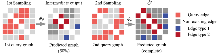
Figure 4: Visualization of the iterative sampling process, with a query edge proportion

4 Experiments

We conduct experiments to present the capability of SparseDiff across a wide range of graphs. SparseDiff matches state-of-the-art performance on datasets of small molecules (QM9, Moses), while being simulatenously very competitive on datasets of larger graphs (Planar, SBM, Protein, Ego). We compare the performance of SparseDiff to GraphNVP (Madhawa et al., 2019), DiGress (Vignac et al., 2023a), Spectre (Martinkus et al., 2022), GraphRNN (You et al., 2018), GG-GAN (Krawczuk et al., 2017), JDSS (Jo et al., 2022), as well as several scalable models: HiGen (Karami, 2023), EDGE (Chen et al., 2023), BiGG (Dai et al., 2020) and HGGT (Jang et al., 2023), and GraphARM (Kong et al., 2023).

4.1 Molecule generation

Since our method admits dense models as a limit when $\lambda=1$, it should match their performance on datasets of small graphs. We verify this capability on the QM9, and Moses molecular datasets used in DiGress (Vignac et al., 2023a). The QM9 dataset (Wu et al., 2018) that contains molecules with up to 9 heavy atoms can either be treated with implicit or explicit hydrogens. The Moses benchmark (Polykovskiy et al., 2020), based on ZINC Clean Leads, contains drug-sized molecules and features many tools to assess the model performance. Since QM9 contains charged atoms, we incorporate formal charges as an additional discrete node feature that is learned during diffusion, similarly to (Vignac et al., 2023b). For fair comparison, we also apply this improvement to DiGress.

Table 1: Molecule generation on QM9 with implicit hydrogens (mean and std over 5 samplings). For fair comparison, DiGress was modified to handle formal charges and benchmarked. While there is no major benefit to using sparsity on small graph, SparseDiff is very competitive, while other scalable models have a poor FCD metric, indicating that they does not correctly model the data.

Class	Method	Valid $(\%)\uparrow$	Unique $(\%)\uparrow$	Connected $(\%)\uparrow$	FCD $\downarrow$
Dense	SPECTRE	$87.3\hskip 11.38092pt$	$35.7\hskip 11.38092pt$	-	-
	GraphNVP	$83.1\hskip 11.38092pt$	$99.2\hskip 11.38092pt$	-	-
	GDSS	$95.7\hskip 11.38092pt$	$98.5\hskip 11.38092pt$	-	-
	DiGress	$99.2\hskip 11.38092pt$	$95.9\hskip 11.38092pt$	$99.5$	$0.15$
	DiGress + charges	$99.3{\scriptstyle\pm{.0}}$	$95.9{\scriptstyle\pm{.2}}$	$99.4{\scriptstyle\pm{.2}}\hskip 7.11317pt$	$0.15{\scriptstyle\pm{.01}}$
Sparse	GraphARM	$90.3\hskip 11.38092pt$	-	-	1.22
	EDGE	$99.1\hskip 11.38092pt$	$\bm{100}\hskip 11.38092pt$	-	$0.46$
	HGGT	$99.2\hskip 11.38092pt$	$95.7\hskip 11.38092pt$	-	0.40
	SparseDiff(ours)	$\bm{99.6}{\scriptstyle\pm{.04}}$	$99.7{\scriptstyle\pm{.01}}$	$\bm{99.7}{\scriptstyle\pm{.02}}$	$\bm{0.11}{\scriptstyle\pm{.01}}$

For QM9 dataset, we assess performance by checking the proportion of connected graphs, the molecular validity of the largest connected component (measured by the success of RDKit sanitization), uniqueness over 10.000 molecules. Additionally, we use the Frechet ChemNet Distance (FCD) (Preuer et al., 2018) which measures the similarity between sets of molecules using a pretrained neural network. In Table 1, we observe that SparseDiff overall achieves the best performance on QM9 with implicit hydrogens. In particular, it clearly outperforms other scalable methods on the FCD metric, showing that such methods are not well suited to small and very structured graphs.

Results for QM9 with explicit hydrogens and the MOSES dataset are presented in Tables 5 (Appendix D.3), and Table 6 (Appendix D.4). We find that SparseDiff compares similarly to the DiGress model, which is expected as small graphs are not very sparse.

4.2 Large graph generation

Table 2: Unconditional generation on the Stochastic Block Model (SBM) and Planar datasets. A SBM graph is valid if it passes a statistical test for the stochastic block model, while a planar graph is valid if it is planar and connected. Results are presented in the form of ratios: $\operatorname{MMD}(\text{generated},\text{test})^{2}/\operatorname{MMD}(\text{train},\text{test})^{2}$. VUN: valid, unique & novel graphs.

Dataset	Stochastic block model				Planar
Model	Deg.$\downarrow$	Clust.$\downarrow$	Orbit$\downarrow$	V.U.N.$\uparrow$	Deg. $\downarrow$	Clust. $\downarrow$	Orbit$\downarrow$	V.U.N.$\uparrow$
GraphRNN	6.9	1.7	3.1	5%	24.5	9.0	2508	0%
GRAN	14.1	1.7	2.1	25%	3.5	1.4	1.8	0%
GG-GAN	4.4	2.1	2.3	25%	–	–	–	–
SPECTRE	1.9	1.6	1.6	53%	2.5	2.5	2.4	25%
DiGress	$\bm{1.6}$	$\bm{1.5}$	1.7	$\bm{74}\%\hskip 7.11317pt$	$\bm{1.4}$	$\bm{1.2}$	$\bm{1.7}$	$75$%
HiGen	2.4	$\bm{1.5}$	$\bm{1.4}$	–	–	–	–	–
SparseDiff	$\bm{2.0}{\scriptstyle\pm{1.6}}$	$\bm{1.5}{\scriptstyle\pm{.0}}$	$\bm{1.4}{\scriptstyle\pm{.1}}$	$56\%{\scriptstyle\pm{8.5}}$	$3.6{\scriptstyle\pm{1.7}}$	$\bm{1.4}{\scriptstyle\pm{.4}}$	$3.4{\scriptstyle\pm{1.2}}$	$\bm{88}\%{\scriptstyle\pm{7}}$

Table 3: Unconditional generation on graphs with up to 500 nodes. On such graphs, dense models such as DiGress clearly fail, whereas SparseDiff presents competitive performance on most metrics. Results are presented in the form of ratios: $\operatorname{MMD}(\text{generated},\text{test})^{2}/\operatorname{MMD}(\text{train},\text{test})^{2}$.

Dataset	Class	Model	Degree $\downarrow$	Clustering $\downarrow$	Orbit $\downarrow$	Spectre $\downarrow$	RBF $\downarrow$
Protein	Dense	GRAN	6.7	7.1	40.6	5.7	–
		DiGress	$18.4{\scriptstyle\pm{2.3}}$	$14.8{\scriptstyle\pm{2.1}}$	$16.0{\scriptstyle\pm{5.5}}$	$5.9{\scriptstyle\pm{1.1}}$	5.2
	Sparse	DRuM	6.3	9.7	10.8	3.3	–
		BiGG	$\bm{0.3}$	3.7	$\bm{7.1}$	5.0	–
		HiGen	4.0	6.4	7.3	2.8	–
		SparseDiff	$10.3{\scriptstyle\pm{1.1}}$	$\bm{3.4}{\scriptstyle\pm{.2}}$	$15.1{\scriptstyle\pm{2.0}}$	$\bm{1.6}{\scriptstyle\pm{.07}}$	$\bm{3.4}{\scriptstyle\pm{.7}}$
Ego	Dense	DiGress	354	$\bm{0.9}$	100	–	5.3
	Sparse	EDGE	290	17.3	43.3	–	4.0
		HiGen	$\bm{9.5}$	4.9	$\bm{2.4}$	$\bm{2.9}$	–
		SparseDiff	$\bm{9.5}{\scriptstyle\pm{3.5}}$	$5.4{\scriptstyle\pm{.2}}$	$\bm{2.5}{\scriptstyle\pm{.1}}$	$\bm{3.6}{\scriptstyle\pm{1.1}}$	$\bm{3.9}{\scriptstyle\pm{1.0}}$

We also evaluate our model on datasets of graphs with increasing size: first, a dataset of Planar graphs (with 64 nodes per graph) which tests the ability of a model to generate graphs without edge crossings. Then, a dataset drawn from the Stochastic Block Model (SBM) (Martinkus et al., 2022) with 2 to 5 communities. SBM graphs contains up to $200$ nodes, which is the largest size used in dense diffusion models such as DiGress (Vignac et al., 2023a). Finally, we use the Ego (Sen et al., 2008) and Protein (Dobson & Doig, 2003) datasets that feature graphs with up to $500$ nodes. Ego is sourced from the CiteSeer (Giles et al., 1998) dataset, captures citation relationships, while Protein represents amino acids connected when they are within 6 Angstroms of each other. Statistics for these datasets can be found in Appendix D.2.

Additionally, MMD metrics, commonly used in graph generation tasks, produce small values that are challenging to directly compare. To address this, we report the metrics divided by $\operatorname{MMD}(\text{training},\text{test})^{2}$, and provide raw numbers in Appendix D.5.

In addition to the MMD metrics, we report the validity of generated graphs for the SBM dataset, which is the fraction of graphs that pass a statistical test for the stochastic block model. For the Planar dataset, validity corresponds to the fraction of graphs that are planar and connected. We also use the RBF MMD metric defined in Thompson et al. (2022), which measures the diversity and fidelity of generated graphs using a randomly parametrized GNN.

Results are presented in Tables 2 and 3. We observe that dense models can achieve very good results on the SBM and planar graphs, which are not too large, but fail on larger graphs. The reason is that a tiny batch size (of 2 on a 32Gb GPU) needs to be used for such graphs, which makes training very slow. SparseDiff is competitive with both dense and scalable models on most metrics of all datasets, despite not being tailored to large graphs only. We however note that evaluation on these datasets is typically done by sampling only a small number of graphs, which makes results very brittle across different samplings from the same model. We therefore strongly advocate for reporting results over several samplings for fair comparison, which should for instance prevent results inferior to $1.0$ from appearing. ‘

5 Conclusion

In this study, we introduce SparseDiff, a scalable discrete denoising diffusion model for graph generation. SparseDiff permits the use of edge list representations by predicting only a subset of edges at once. Experimental results demonstrate that SparseDiff exhibits very good performance across all graph sizes, whereas other scalable methods tend to perform poorly on small, structured graphs. SparseDiff enhances the capabilities of discrete diffusion models to process larger datasets, thereby broadening its applicability, including tasks such as generating large biological molecules and community graphs, among others.

Appendix A Algorithm

A.1 Generation Algorithm

In the process of graph generation, we employ an iterative approach to construct the adjacency matrix. During each iteration, a random set of query edges, counting a proportion denoted by $\lambda$, is drawn without repetition from all edges until the entire matrix is populated. It is worth noting that when $\lambda$ does not evenly divide 1, the last iteration may result in a different number of query edges. To maintain consistency in the number of query edges, we adopt a strategy in such cases: we utilize the last $\lambda$ percent of edges from the dataset. This suggests that a small portion of edges will be repeatedly sampled during generation, but given that their predicted distribution should remain the same, this strategy will not change any mathematical formulation behind. Besides, the nodes are only sampled once across all iterations. To enhance clarity and facilitate understanding, we provide Algorithm 1 as the following.

Sample the number of nodes $n$ from the training data distribution

Sample $G^{T}\sim q_{\bm{X}}(n)\times q_{\bm{Y}}(n)$ $\triangleright$ Random graph

for t = T to 1 do

       Permute ${\bm{E}}(n)$ $\triangleright$ Permuted list of all pairs between $n$ nodes

       Partition ${\bm{E}}(n)$ to ${\bm{E}}_{p}=[{\bm{E}}_{1},...,{\bm{E}}_{1/\lambda}]$

       Create the empty graph $G_{t-1}$

       for i = 1 to $1/\lambda$ do

             Obtain the query graph $G_{q}$ from ${\bm{E}}_{p}$ $\triangleright$ $G_{q}$ contains edges in ${\bm{E}}_{p}[i]$

             $z\leftarrow f(G^{t},t)$ $\triangleright$ Optional: structural and spectral encoding

             $\hat{p}^{\bm{X}},\hat{p}^{\bm{Y}}_{q}\leftarrow\phi_{\theta}(G^{t},G_{q},z)$ $\triangleright$ Sparse forward pass

             Sample query edge labels ${\bm{Y}}^{q}$ according to $\hat{p}^{\bm{Y}}_{q}$

             Add ${\bm{Y}}^{q}_{existing}$ to $G^{t-1}$ $\triangleright$ Only add existing edges to keep sparsity

             if i==0 then

                   Sample node labels ${\bm{X}}$ according to $\hat{p}^{\bm{X}}$

                   Update ${\bm{X}}$ to $G^{t-1}$ $\triangleright$ Update nodes only once

                  

             end if

            

       end for

      

end for

return $G^{0}$

Algorithm 1 Sampling from SparseDiff

A.2 Sparse noise model

We design a special algorithm to apply noise to graph data in a sparse manner. The fundamental idea behind this algorithm is to treat separately existing and non-existing edges. In sparse graphs, the number of edges typically scales sub-quadratically with the number of nodes, denoted as $n$, while the quadratic space complexity mainly stems from the non-existing edges. Even after sampling, newly emerging edges (those transitioning from non-existing to existing) also exhibit a linear scale concerning $n$. Thus, we initially employ binomial sampling to estimate the count of these emerging edges denoted as $m_{new}$. Subsequently, we randomly select $m_{new}$ edges from the pool of all non-existing edges and assign them random labels following the noised edge distribution, while the remaining non-existing edges maintain their non-existent state. This algorithm enables the replication of the traditional diffusion process without necessitating the adjacency matrix of size $n^{2}$, but only with the edge list composed by $m^{t}+m_{new}$ edges. The most challenging aspect of this algorithm is the random selection of a specific number (i.e. $m_{new}$) of emerging edges from the entire set of non-existing edges without introducing the adjacency matrix. Due to the algorithm’s complexity and the technical intricacies involved, a more detailed discussion is discussed later in Appendix A.4.

A.3 Uniform edges sampling for batched graphs

In the context of sparse training, we assume that maintaining the same distribution of edge types as in dense graphs within each graph is beneficial for training. To illustrate, consider a graph where non-existent edges account for $90\%$ of the total edges. In sparse training, on average, the non-existent edges should also constitute $90\%$ of the query edges ${\bm{E}}_{q}$. This assumption implies that we need to perform query edge sampling separately for each graph in order to maintain the distribution within each graph. When a batch contains graphs of varying sizes, simultaneously selecting a proportion of $\tau$ query edges in each graph is not straightforward. For this purpose, an efficient sampling algorithm has been devised and can be viewed in our codes later.

We also apply a permutation to the node ordering in each graph. The absence of this step can negatively impact training performance due to symmetry.

A.4 Uniform Sampling for non-existing edges

When sampling non-existing edges, a common approach is to use the adjacency matrix, which can be problematic for large graphs due to its quadratic size. The same challenge arises in the final step of sampling sparse noise.

Consider a graph with $5$ nodes, featuring $4$ existing edges and $6$ pairs of nodes that are not connected. The condensed indices of the existing edges are $0$, $3$, $4$, and $6$. If the objective is to sample $2$ non-existing edges, you can start by randomly selecting two indices from the range $[0,...,5]$, which corresponds to the 6 non-existing edges. For example, if indices $[2,3]$ are randomly chosen, where $2$ denotes the position of the third non-existing edge, and $3$ represents the fourth non-existing edge. These condensed indices are then inserted in the list of non-existing edges. Upon amalgamation with the existing edges, the final set of edges will become $[5,7]$. This approach allows us to efficiently sample non-existing edges while ensuring the proper placement of existing edges within the sampled set. Given the high complexity of the coding, please refer to our codes for more details.

Appendix B Proof of Lemma 3.1

The lemma for noisy graph with guaranteed sparsity comes from directly from the proposition regarding the tail behavior of a binomial distribution (Desolneux et al., 2008) as follows:

Proposition B.1.

(Tail behavior of a binomial distribution)

Let $X_{i},i=1,...l$ be independent Bernoulli random variables with parameter $0<p<\frac{1}{4}$ and let $S_{l}=\sum^{l}_{i=1}X_{i}$. Consider a constant $p<r<1$ or a real function $p<r(l)<1$. Then according to the Hoeffding inequality, $\mathcal{B}(l,k,p)=\mathbb{P}[S_{l}\geq k]$ satisfies:

$$-\frac{1}{l}log\mathcal{P}[S_{l}\geq rl]\geq rlog\frac{r}{p}+(1-p)log\frac{1-r}{1-p}$$ (2)

For sparse graphs, the edge ratio $k$ is clearly smaller than $\frac{1}{4}$. Consider then Bernoulli random variables with parameter $k$ and a constant $k<r<1$ with $n(n-1)/2$ (i.e. number of all node pairs in an undirected graph) draws, and note sampled existing edge number $S_{n(n-1)/2}$ as $m_{t}$, we have:

$$log(\mathbb{P}[\frac{m_{t}}{n(n-1)/2}\geq r])\leq-\frac{n(n-1)}{2}[rlog\frac{r}{k}+(1-k)log\frac{1-r}{1-k}]$$ (3)

Appendix C Structural and Positional Encodings

During training, we augment model expressiveness with additional encodings. To make thing clear, we divide them into encodings for edges, for nodes, and for graphs.

Encoding for graphs

We first incorporate graph eigenvalues, known for their critical structural insights, and cycle-counts, addressing message-passing neural networks’ inability to detect cycles (Chen et al., 2020). The first requires $n^{3}$ operations for matrix decomposition, the second $n^{2}$ for matrix multiplication, but both are optional in our model and do not significantly limit scalability even with graphs up to size $500$. In addition to the previously mentioned structural encodings, we integrate the degree distribution to enhance the positional information within the graph input, which is particularly advantageous for graphs with central nodes or multiple communities. Furthermore, for graphs featuring attributed nodes and edges, the inclusion of node type and edge type distributions also provides valuable benefits.

Encoding for nodes

At the node level, we utilize graph eigenvectors, which are fundamental in graph theory, offering valuable insights into centrality, connectivity, and diverse graph properties.

Encoding for edges

To aid in edge label prediction, we introduce auxiliary structural encodings related to edges. These include the shortest distance between nodes and the Adamic-Adar index. The former enhances node interactions, while the latter focuses on local neighborhood information. Due to computational constraints, we consider information within a 10-hop radius, categorizing it as local positional information.

Molecular information

In molecular datasets, we augment node features by incorporating edge valency and atom weights. Additionally, formal charge information is included as an additional node label for diffusion and denoising during training, as formal charges have been experimentally validated as valuable information (Vignac et al., 2023b).

Appendix D Additional Experiments

D.1 MMD metrics

In our research, we carefully select specific metrics tailored to each dataset, with a primary focus on four widely recognized Maximum Mean Discrepancy (MMD) metrics. These metrics utilize the total variation (TV) distance, as detailed in (Martinkus et al., 2022). They encompass node degree (Deg), clustering coefficient (Clus), orbit count (Orb), and graph spectra (Spec). The first three local metrics compare the degree distributions, clustering coefficient distributions, and the occurrence of all 4-node orbits within graphs between the generated and training samples. Additionally, we extend our analysis to include the comparison of graph spectra by computing the eigenvalues of the normalized graph Laplacian, providing complementary insights into the global properties of the graphs.

D.2 Statistics of the datasets

To provide a more comprehensive overview of the various scales found in existing graph datasets, we present here key statistics for them. These statistics encompass the number of graphs, the range of node numbers, the range of edge numbers, the edge fraction for existing edges, and the query edge proportion $\lambda$ used for training, i.e. the proportion of existing edges among all node pairs. In our consideration, we focus on undirected graphs. Therefore, when counting edges between nodes $i$ and $j$, we include the edge in both directions.

Table 4: Statistics for the datasets employed in our experiments.

Name	Graph number	Node range	Edge range	Edge Fraction ($\%$)	$\lambda$ ($\%$)
QM9	133,885	[2,9]	[2, 28]	[20, 56]	50
QM9(H)	133,885	[3, 29]	[4, 56]	[7.7, 44]	50
Moses	1,936,962	[8, 27]	[14, 62]	[8.0, 22]	50
Planar	200	[64, 64]	[346, 362]	[8.4, 8.8]	50
SBM	200	[44, 187]	[258, 2258]	[6.0, 17]	25
Ego	757	[50, 399]	[112, 2124]	[1.2, 11]	10
Protein	918	[100, 500]	[372, 3150]	[8.9, 6.7]	10

D.3 QM9 with explicit hydrogens

We additionally report the results for QM9 with explicit hydrogens in Table 5. Having explicit hydrogens makes the problem more complex because the resulting graphs are larger. We observe that SparseDiff achieves better validity than DiGress and has comparable results on other metrics when both are utilizing charges.

Table 5: Unconditional generation on QM9 with explicit hydrogens. On small graphs such as QM9, sparse models are not beneficial, but SparseDiff still achieves very good performance.

Model	Connected	Valid$\uparrow$	Unique$\uparrow$	Atom stable$\uparrow$	Mol stable$\uparrow$
DiGress	–	$95.4$	$97.6$	$98.1$	$79.8$
DiGress + charges	98.6	97.7	$96.9$	99.8	97.0
SparseDiff	98.1	$97.9$	$96.9$	99.7	95.7

D.4 MOSES benchmark evaluation

Moses is an extensive molecular dataset with larger molecular graphs than QM9, offering a much more comprehensive set of metrics. While autoregressive models such as GraphINVENT are recognized for achieving higher validity on this dataset, both SparseDiff and DiGress exhibit advantages across most other metrics. Notably, SparseDiff closely aligns with the results achieved by DiGress, affirming the robustness of our method on complex datasets.

Table 6: Mean and standard deviation across 5 samplings on the MOSES benchmark. SparseDiff has similar performance to DiGress, despite a shorter training time.

Model	Connected $\uparrow$	Valid $(\%)\uparrow$	Unique $(\%)\uparrow$	Novel $(\%)\uparrow$	Filters $(\%)\uparrow$
GraphINVENT	–	$\bm{96.4}\hskip 12.23447pt$	$99.8\hskip 12.23447pt$	–	$95.0\hskip 12.23447pt$
DiGress	–	$85.7\hskip 11.38092pt$	$\bm{100.0}\hskip 12.23447pt$	$95.0\hskip 12.23447pt$	$\bm{97.1}\hskip 12.23447pt$
SparseDiff	$98.2{\scriptstyle\pm{.0}}$	$86.7{\scriptstyle\pm{.2}}$	$\bm{100.0}{\scriptstyle\pm{.0}}$	$\bm{96.3}{\scriptstyle\pm{.1}}$	$96.7{\scriptstyle\pm{.1}}$
Model	FCD $\downarrow$	SNN $(\%)\uparrow$	Scaf $(\%)\uparrow$	Frag $(\%)\uparrow$	IntDiv $(\%)\uparrow$
GraphINVENT	$1.22\hskip 15.6491pt$	$\bm{53.9}\hskip 11.38092pt$	$12.7\hskip 15.6491pt$	$98.6\hskip 12.23447pt$	$\bm{85.7}\hskip 12.23447pt$
DiGress	$\bm{1.19}\hskip 15.6491pt$	$52.2\hskip 11.38092pt$	$\bm{14.8}\hskip 15.6491pt$	$\bm{99.6}\hskip 12.23447pt$	$85.3\hskip 12.23447pt$
SparseDiff	$1.35{\scriptstyle\pm{.02}}$	$51.0{\scriptstyle\pm{.0}}$	$14.2{\scriptstyle\pm{1.7}}$	$\bm{99.6}{\scriptstyle\pm{.0}}$	$85.5{\scriptstyle\pm{.0}}$
Model	Filters $(\%)\uparrow$	logP $(e^{-2})\downarrow$	SA $\downarrow$	QED $(e^{-3})\downarrow$	Weight $(\%)\downarrow$
GraphINVENT	$95.0\hskip 12.23447pt$	$\bm{0.67}\hskip 8.5359pt$	$4.5\hskip 12.23447pt$	$\bm{0.25}\hskip 15.6491pt$	$16.1\hskip 12.23447pt$
DiGress	$\bm{97.1}\hskip 12.23447pt$	$3.4\hskip 12.23447pt$	$\bm{3.6}\hskip 12.23447pt$	$2.91\hskip 15.6491pt$	$1.42\hskip 11.38092pt$
SparseDiff	$96.7{\scriptstyle\pm{.1}}$	$8.0{\scriptstyle\pm{.4}}$	$7.9{\scriptstyle\pm{.3}}$	$4.17{\scriptstyle\pm{.33}}$	$\bm{1.25}{\scriptstyle\pm{.1}}$

D.5 Raw results

To ease comparison with other methods, Table 7 provides the raw numbers (not presented as ratios) for the SBM, Planar, Ego, and Protein datasets. Not that this table contains the FID metrics from (Thompson et al., 2022), that we did not include in the main text. The reason is that we found this metric to be very brittle, with some evaluations giving a very large value that would dominate the mean results.

Table 7: Raw results on the SBM, Planar, Protein and Ego datasets.

Model	Deg (e-3)$\downarrow$	Clus (e-2)$\downarrow$	Orb (e-2)$\downarrow$	Spec (e-3)$\downarrow$	FID$\downarrow$	RBF MMD (e-2)$\uparrow$
SBM
Training set	0.8	3.32	2.55	5.2	16.83	3.13
SparseDiff	$1.6{\scriptstyle\pm{1.3}}$	$4.97{\scriptstyle\pm{0.04}}$	$3.46{\scriptstyle\pm{0.04}}$	$4.3{\scriptstyle\pm{0.7}}$	$5.71{\scriptstyle\pm{7.01}}$	$5.04{\scriptstyle\pm{0.21}}$
Planar
Training set	0.2	3.10	0.05	6.3	0.19	3.20
SparseDiff	$0.7{\scriptstyle\pm{0.4}}$	$4.47{\scriptstyle\pm{1.38}}$	$0.17{\scriptstyle\pm{0.06}}$	$6.8{\scriptstyle\pm{0.8}}$	$4.51{\scriptstyle\pm{1.76}}$	$5.27{\scriptstyle\pm{0.50}}$
Protein
Training set	0.3	0.68	0.32	0.9	5.74	0.68
SparseDiff	$3.1{\scriptstyle\pm{0.0}}$	$2.28{\scriptstyle\pm{0.10}}$	$4.82{\scriptstyle\pm{.64}}$	$1.4{\scriptstyle\pm{.1}}$	$4.83{\scriptstyle\pm{1.48}}$	$2.29{\scriptstyle\pm{.48}}$
Ego
Training set	0.2	1.0	1.20	1.4	1.21	1.23
SparseDiff	$1.9{\scriptstyle\pm{0.7}}$	$5.37{\scriptstyle\pm{0.24}}$	$2.09{\scriptstyle\pm{.17}}$	$5.0{\scriptstyle\pm{1.5}}$	$16.15{\scriptstyle\pm{12.86}}$	$4.83{\scriptstyle\pm{1.18}}$

D.6 Ablations

This part presents 2 ablation experiments that motivate our approach. SparseDiff builds upon an experimental observation and a hypothesis. Firstly, our experiments demonstrate that relying solely on node features for link prediction yields unsatisfactory results. This observation encouraged us to design the computational graph that contains all edges to be predicted (i.e. query edges) as the input graph. Secondly, we hypothesized that preserving the same distribution of edge types as observed in dense graphs for loss calculation is advantageous for training. This hypothesis requires to only calculate losses on uniformly sampled query edges.

D.6.1 Link Prediction

Table 8: Influence of including edges features for edge prediction.

Model	Deg $\downarrow$	Clus $\downarrow$	Orb$\downarrow$	Spec$\downarrow$	FID$\downarrow$	RBF MMD$\downarrow$
Link Pred	0.0043	0.0721	0.0275	0.0344	1.51e6	0.0315
SparseDiff	$\textbf{0.0019}{\scriptstyle\pm{.00}}$	$\bm{0.0537}{\scriptstyle\pm{.00}}$	$0.0299{\scriptstyle\pm{.00}}$	$\bm{0.0050}{\scriptstyle\pm{.00}}$	$\bm{16.1}{\scriptstyle\pm{12.9}}$	$0.0483{\scriptstyle\pm{.01}}$

In this experiment, we intentionally avoided to use easily learnable molecular datasets that come with rich supplementary encodings. Instead, we chose to conduct the experiments on a large dataset, namely Ego, to assess their performance. In Table 8, a model that does not specifically include edge features for edge prediction performs much worse on all metrics except on RBF MMD and orbit. This observation shows that, despite that a model can also leverage the information of existing edges into node features, the lack of non-existing edges participating directly in training still ruins its performance.

D.6.2 Query edges with proper distribution

Table 9: Influence of edge loss distribution on EGO dataset.

Loss based on	Deg $\downarrow$	Clus $\downarrow$	Orb$\downarrow$	Spec$\downarrow$	FID$\downarrow$	RBF MMD$\downarrow$
Comp graph	0.0021	0.0566	$\bm{0.0270}$	0.0100	28.2	$\bm{0.0396}$
Query graph	$\textbf{0.0019}{\scriptstyle\pm{.00}}$	$\bm{0.0537}{\scriptstyle\pm{.00}}$	$0.0299{\scriptstyle\pm{.00}}$	$\bm{0.0050}{\scriptstyle\pm{.00}}$	$\bm{16.1}{\scriptstyle\pm{12.9}}$	$0.0483{\scriptstyle\pm{.01}}$

In order to emphasize the importance of preserving the edge distribution when computing losses, we conduct an experiment where we assess the performance of a model trained using all computational edges as opposed to solely using query edges. The former results in an increased emphasis on existing edges during training compared to SparseDiff. Similarly, we use the Ego dataset for initial experiments. Table 9 shows that using edges of the computational graph $G_{c}$ results in worse performance on most of the metrics, which indicates the importance of keeping a balanced edge distribution for loss calculation.

Appendix E Visualization

(a) Training graphs.

(b) Generated graphs.

Figure 5: Visualization for Moses dataset.

(a) Training graphs.

(b) Generated graphs.

Figure 6: Visualization for Planar dataset.

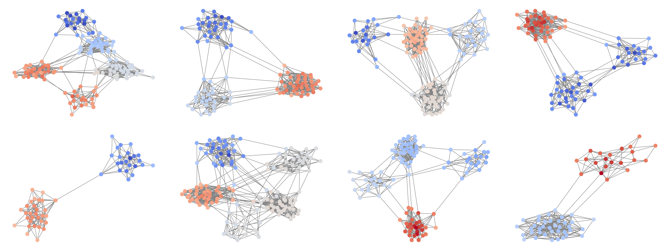
(a) Training graphs.

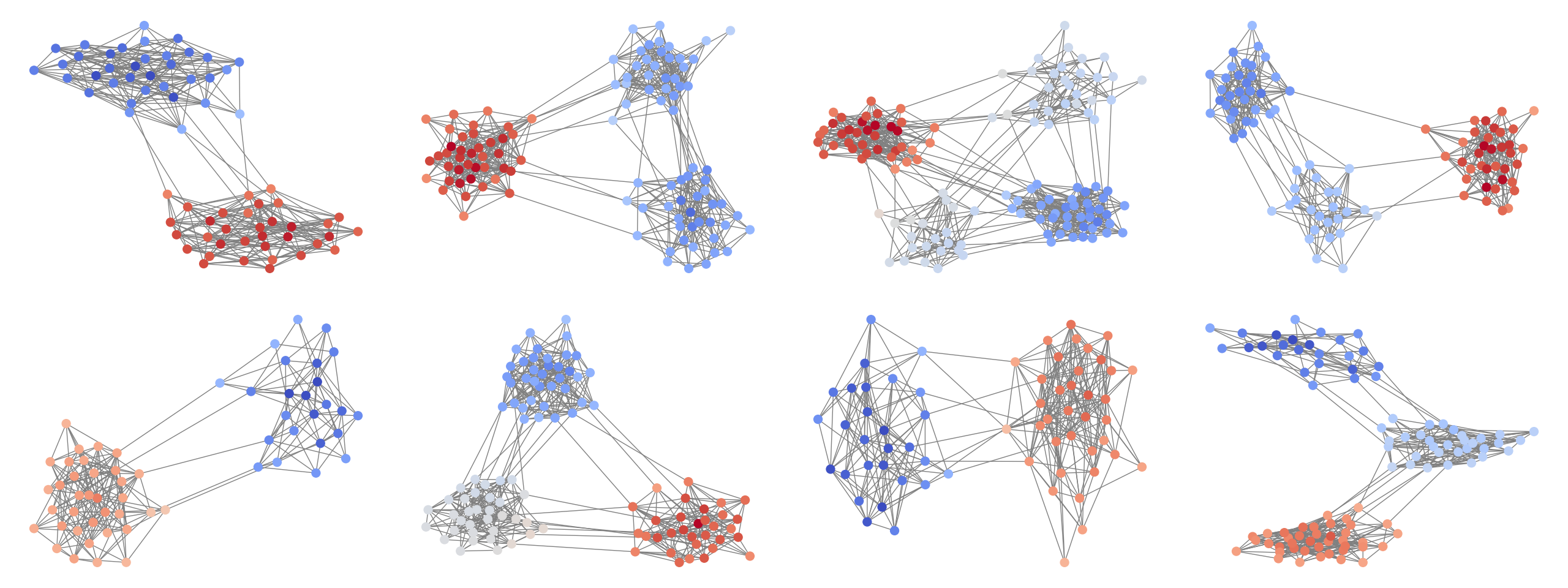
(b) Generated graphs.

Figure 7: Visualization for SBM dataset.

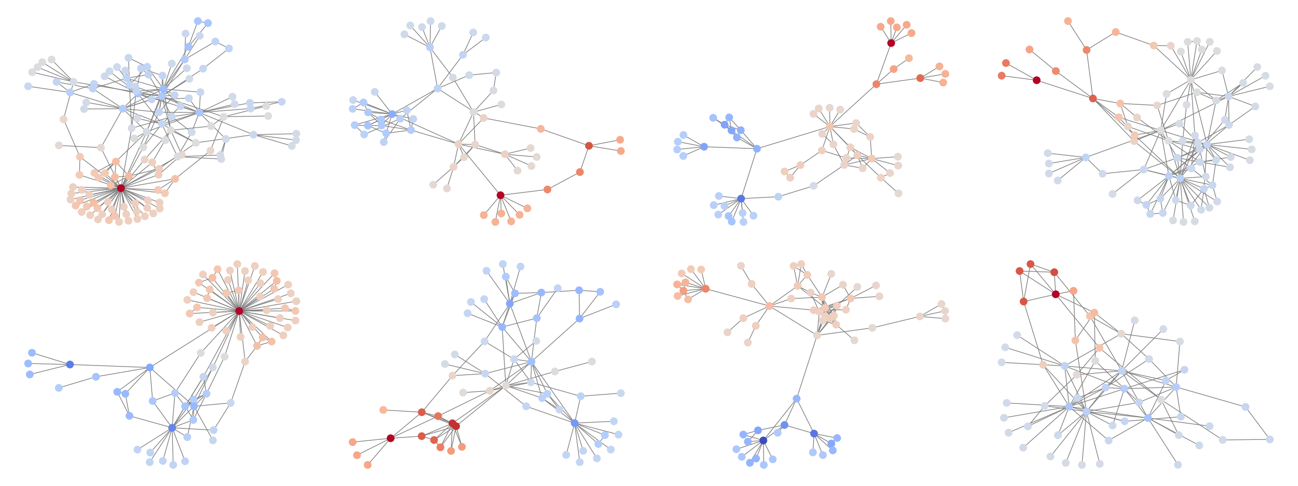
(a) Training graphs.

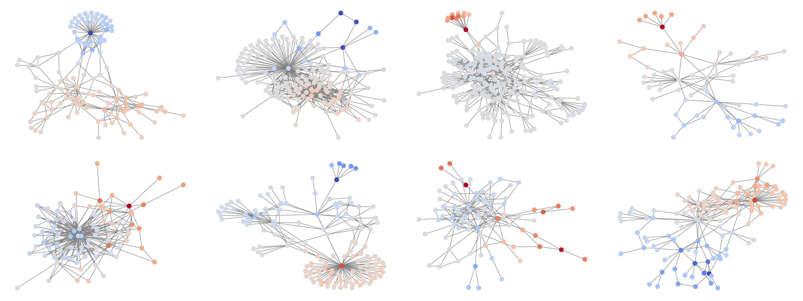
(b) Generated graphs.

Figure 8: Visualization for Ego dataset.

(a) Training graphs.

(b) Generated graphs.

Figure 9: Visualization for Protein dataset.

References

- Aiello et al. (2000) William Aiello, Fan Chung, and Linyuan Lu. A random graph model for massive graphs. In ACM Symposium on Theory of computing, 2000.
- Alon & Yahav (2020) Uri Alon and Eran Yahav. On the bottleneck of graph neural networks and its practical implications. arXiv preprint arXiv:2006.05205, 2020.
- Austin et al. (2021) Jacob Austin, Daniel Johnson, Jonathan Ho, Daniel Tarlow, and Rianne van den Berg. Structured denoising diffusion models in discrete state-spaces. In Advances in Neural Information Processing Systems, volume 34, 2021.
- Baek et al. (2021) Minkyung Baek, Frank DiMaio, Ivan Anishchenko, Justas Dauparas, Sergey Ovchinnikov, Gyu Rie Lee, Jue Wang, Qian Cong, Lisa N Kinch, R Dustin Schaeffer, et al. Accurate prediction of protein structures and interactions using a three-track neural network. Science, 373(6557):871–876, 2021.
- Barabási (2013) Albert-László Barabási. Network science. Philosophical Transactions of the Royal Society A: Mathematical, Physical and Engineering Sciences, 371(1987), 2013.
- Boschin (2023) Armand Boschin. Machine learning techniques for automatic knowledge graph completion. PhD thesis, Institut polytechnique de Paris, 2023.
- Chamberlain et al. (2022) Benjamin Paul Chamberlain, Sergey Shirobokov, Emanuele Rossi, Fabrizio Frasca, Thomas Markovich, Nils Hammerla, Michael M Bronstein, and Max Hansmire. Graph neural networks for link prediction with subgraph sketching. arXiv preprint arXiv:2209.15486, 2022.
- Chen et al. (2023) Xiaohui Chen, Jiaxing He, Xu Han, and Li-Ping Liu. Efficient and degree-guided graph generation via discrete diffusion modeling. arXiv preprint arXiv:2305.04111, 2023.
- Chen et al. (2020) Zhengdao Chen, Lei Chen, Soledad Villar, and Joan Bruna. Can graph neural networks count substructures? In Advances in neural information processing systems, volume 33, 2020.
- Corso et al. (2020) Gabriele Corso, Luca Cavalleri, Dominique Beaini, Pietro Liò, and Petar Veličković. Principal neighbourhood aggregation for graph nets. Advances in Neural Information Processing Systems, 2020.
- Dai et al. (2020) Hanjun Dai, Azade Nazi, Yujia Li, Bo Dai, and Dale Schuurmans. Scalable deep generative modeling for sparse graphs. In International Conference on Machine Learning. PMLR, 2020.
- De Cao & Kipf (2018) Nicola De Cao and Thomas Kipf. Molgan: An implicit generative model for small molecular graphs. In ICML Workshop on Theoretical Foundations and Applications of Deep Generative Models, 2018.
- Desolneux et al. (2008) Agnés Desolneux, Lionel Moisan, and Jean-Michel Morel. Estimating the binomial tail. From Gestalt Theory to Image Analysis: A Probabilistic Approach, pp. 47–63, 2008.
- Dhariwal & Nichol (2021) Prafulla Dhariwal and Alexander Nichol. Diffusion models beat gans on image synthesis. In Advances in Neural Information Processing Systems, 2021.
- Di Giovanni et al. (2023) Francesco Di Giovanni, Lorenzo Giusti, Federico Barbero, Giulia Luise, Pietro Lio, and Michael M. Bronstein. On over-squashing in message passing neural networks: The impact of width, depth, and topology. In Proceedings of the 40th International Conference on Machine Learning, 2023.
- Dobson & Doig (2003) Paul D. Dobson and Andrew J. Doig. Distinguishing enzyme structures from non-enzymes without alignments. Journal of molecular biology, 2003.
- Erdős et al. (1960) Paul Erdős, Alfréd Rényi, et al. On the evolution of random graphs. Publ. math. inst. hung. acad. sci, 1960.
- Fey & Lenssen (2019) Matthias Fey and Jan Eric Lenssen. Fast graph representation learning with pytorch geometric. arXiv preprint arXiv:1903.02428, 2019.
- Giles et al. (1998) C. Lee Giles, Kurt D. Bollacker, and Steve Lawrence. Citeseer: An automatic citation indexing system. In Proceedings of the Third ACM Conference on Digital Libraries. Association for Computing Machinery, 1998.
- Gilmer et al. (2017) Justin Gilmer, Samuel S Schoenholz, Patrick F Riley, Oriol Vinyals, and George E Dahl. Neural message passing for quantum chemistry. In International conference on machine learning. PMLR, 2017.
- Haefeli et al. (2022) Kilian Konstantin Haefeli, Karolis Martinkus, Nathanaël Perraudin, and Roger Wattenhofer. Diffusion models for graphs benefit from discrete state spaces. arXiv preprint arXiv:2210.01549, 2022.
- Ho et al. (2020) Jonathan Ho, Ajay Jain, and Pieter Abbeel. Denoising diffusion probabilistic models. In Advances in Neural Information Processing Systems. Curran Associates, Inc., 2020.
- Ho et al. (2022) Jonathan Ho, William Chan, Chitwan Saharia, Jay Whang, Ruiqi Gao, Alexey Gritsenko, Diederik P Kingma, Ben Poole, Mohammad Norouzi, David J Fleet, et al. Imagen video: High definition video generation with diffusion models. arXiv preprint arXiv:2210.02303, 2022.
- Hoogeboom et al. (2021) Emiel Hoogeboom, Didrik Nielsen, Priyank Jaini, Patrick Forré, and Max Welling. Argmax flows and multinomial diffusion: Learning categorical distributions. In Advances in Neural Information Processing Systems, volume 34, 2021.
- Ingraham et al. (2022) John Ingraham, Max Baranov, Zak Costello, Vincent Frappier, Ahmed Ismail, Shan Tie, Wujie Wang, Vincent Xue, Fritz Obermeyer, Andrew Beam, et al. Illuminating protein space with a programmable generative model. bioRxiv, 2022.
- Jang et al. (2023) Yunhui Jang, Dongwoo Kim, and Sungsoo Ahn. Hierarchical graph generation with k2-trees. arXiv preprint arXiv:2305.19125, 2023.
- Jin et al. (2018) Wengong Jin, Regina Barzilay, and Tommi Jaakkola. Junction tree variational autoencoder for molecular graph generation. In International conference on machine learning. PMLR, 2018.
- Jin et al. (2020) Wengong Jin, Regina Barzilay, and Tommi Jaakkola. Hierarchical generation of molecular graphs using structural motifs. In International Conference on Machine Learning. PMLR, 2020.
- Jo et al. (2022) Jaehyeong Jo, Seul Lee, and Sung Ju Hwang. Score-based generative modeling of graphs via the system of stochastic differential equations. arXiv preprint arXiv:2202.02514, 2022.
- Karami (2023) Mahdi Karami. Higen: Hierarchical graph generative networks. arXiv preprint arXiv:2305.19337, 2023.
- Kingma et al. (2021) Diederik Kingma, Tim Salimans, Ben Poole, and Jonathan Ho. Variational diffusion models. Advances in neural information processing systems, 2021.
- Kong et al. (2023) Lingkai Kong, Jiaming Cui, Haotian Sun, Yuchen Zhuang, B. Aditya Prakash, and Chao Zhang. Autoregressive diffusion model for graph generation, 2023. URL https://openreview.net/forum?id=98J48HZXxd5.
- Kong et al. (2020) Zhifeng Kong, Wei Ping, Jiaji Huang, Kexin Zhao, and Bryan Catanzaro. Diffwave: A versatile diffusion model for audio synthesis. arXiv preprint arXiv:2009.09761, 2020.
- Krawczuk et al. (2017) Igor Krawczuk, Pedro Abranches, Andreas Loukas, and Volkan Cevher. Gg-gan: A geometric graph generative adversarial network. arXiv preprint arXiv:1711.0826, 2017.
- Li et al. (2023) Xujia Li, Yuan Li, Xueying Mo, Hebing Xiao, Yanyan Shen, and Lei Chen. Diga: Guided diffusion model for graph recovery in anti-money laundering. In Proceedings of the 29th ACM SIGKDD Conference on Knowledge Discovery and Data Mining, 2023.
- Liao et al. (2019) Renjie Liao, Yujia Li, Yang Song, Shenlong Wang, Charlie Nash, William L. Hamilton, David Duvenaud, Raquel Urtasun, and Richard Zemel. Efficient graph generation with graph recurrent attention networks. In NeurIPS, 2019.
- Limnios et al. (2023) Stratis Limnios, Praveen Selvaraj, Mihai Cucuringu, Carsten Maple, Gesine Reinert, and Andrew Elliott. Sagess: Sampling graph denoising diffusion model for scalable graph generation. arXiv preprint arXiv:2306.16827, 2023.
- Liu et al. (2018) Qi Liu, Miltiadis Allamanis, Marc Brockschmidt, and Alexander Gaunt. Constrained graph variational autoencoders for molecule design. Advances in neural information processing systems, 31, 2018.
- Madhawa et al. (2019) Kaushalya Madhawa, Katushiko Ishiguro, Kosuke Nakago, and Motoki Abe. Graphnvp: An invertible flow model for generating molecular graphs. arXiv preprint arXiv:1905.11600, 2019.
- Maehara & Rödl (1990) Hiroshi Maehara and Vojtech Rödl. On the dimension to represent a graph by a unit distance graph. In Graphs and Combinatorics. Springer, 1990.
- Martinkus et al. (2022) Karolis Martinkus, Andreas Loukas, Nathanaël Perraudin, and Roger Wattenhofer. Spectre: Spectral conditioning helps to overcome the expressivity limits of one-shot graph generators. arXiv preprint arXiv:2204.01613, 2022.
- Maziarz et al. (2022) Krzysztof Maziarz, Henry Richard Jackson-Flux, Pashmina Cameron, Finton Sirockin, Nadine Schneider, Nikolaus Stiefl, Marwin Segler, and Marc Brockschmidt. Learning to extend molecular scaffolds with structural motifs. In International Conference on Learning Representations (ICLR), 2022.
- Mercado et al. (2021) Rocío Mercado, Tobias Rastemo, Edvard Lindelöf, Günter Klambauer, Ola Engkvist, Hongming Chen, and Esben Jannik Bjerrum. Graph networks for molecular design. Machine Learning: Science and Technology, 2021.
- Niu et al. (2020) Chenhao Niu, Yang Song, Jiaming Song, Shengjia Zhao, Aditya Grover, and Stefano Ermon. Permutation invariant graph generation via score-based generative modeling. In International Conference on Artificial Intelligence and Statistics. PMLR, 2020.
- Perez et al. (2018) Ethan Perez, Florian Strub, Harm De Vries, Vincent Dumoulin, and Aaron Courville. Film: Visual reasoning with a general conditioning layer. In Proceedings of the AAAI Conference on Artificial Intelligence, volume 32, 2018.
- Polykovskiy et al. (2020) Daniil Polykovskiy, Alexander Zhebrak, Benjamin Sanchez-Lengeling, Sergey Golovanov, Oktai Tatanov, Stanislav Belyaev, Rauf Kurbanov, Aleksey Artamonov, Vladimir Aladinskiy, Mark Veselov, et al. Molecular sets (moses): a benchmarking platform for molecular generation models. In Frontiers in pharmacology. Frontiers Media SA, 2020.
- Poole et al. (2022) Ben Poole, Ajay Jain, Jonathan T Barron, and Ben Mildenhall. Dreamfusion: Text-to-3d using 2d diffusion. arXiv preprint arXiv:2209.14988, 2022.
- Preuer et al. (2018) Kristina Preuer, Philipp Renz, Thomas Unterthiner, Sepp Hochreiter, and Gunter Klambauer. Fréchet chemnet distance: a metric for generative models for molecules in drug discovery. Journal of chemical information and modeling, 58(9):1736–1741, 2018.
- Rong et al. (2023) Can Rong, Jingtao Ding, Zhicheng Liu, and Yong Li. City-wide origin-destination matrix generation via graph denoising diffusion. arXiv preprint arXiv:2306.04873, 2023.
- Scarselli et al. (2008) Franco Scarselli, Marco Gori, Ah Chung Tsoi, Markus Hagenbuchner, and Gabriele Monfardini. The graph neural network model. In IEEE transactions on neural networks. IEEE, 2008.
- Sen et al. (2008) Prithviraj Sen, Galileo Namata, Mustafa Bilgic, Lise Getoor, Brian Gallagher, and Tina Eliassi-Rad. Collective classification in network data. In The AI Magazine, 2008.
- Shi et al. (2020) Yunsheng Shi, Zhengjie Huang, Shikun Feng, Hui Zhong, Wenjin Wang, and Yu Sun. Masked label prediction: Unified message passing model for semi-supervised classification. arXiv preprint arXiv:2009.03509, 2020.
- Simonovsky & Komodakis (2018) Martin Simonovsky and Nikos Komodakis. Graphvae: Towards generation of small graphs using variational autoencoders. In International conference on artificial neural networks. Springer, 2018.
- Sohl-Dickstein et al. (2015) Jascha Sohl-Dickstein, Eric A. Weiss, Niru Maheswaranathan, and Surya Ganguli. Deep unsupervised learning using nonequilibrium thermodynamics. In Proceedings of the 32nd International Conference on Machine Learning, ICML, 2015.
- Song et al. (2020) Yang Song, Jascha Sohl-Dickstein, Diederik P Kingma, Abhishek Kumar, Stefano Ermon, and Ben Poole. Score-based generative modeling through stochastic differential equations. arXiv preprint arXiv:2011.13456, 2020.
- Thompson et al. (2022) Rylee Thompson, Boris Knyazev, Elahe Ghalebi, Jungtaek Kim, and Graham W Taylor. On evaluation metrics for graph generative models. arXiv preprint arXiv:2201.09871, 2022.
- Topping et al. (2021) Jake Topping, Francesco Di Giovanni, Benjamin Paul Chamberlain, Xiaowen Dong, and Michael M Bronstein. Understanding over-squashing and bottlenecks on graphs via curvature. arXiv preprint arXiv:2111.14522, 2021.
- Veličković et al. (2017) Petar Veličković, Guillem Cucurull, Arantxa Casanova, Adriana Romero, Pietro Lio, and Yoshua Bengio. Graph attention networks. arXiv preprint arXiv:1710.10903, 2017.
- Vignac et al. (2023a) Clement Vignac, Igor Krawczuk, Antoine Siraudin, Bohan Wang, Volkan Cevher, and Pascal Frossard. Digress: Discrete denoising diffusion for graph generation. In The Eleventh International Conference on Learning Representations, 2023a.
- Vignac et al. (2023b) Clément Vignac, Nagham Osman, Laura Toni, and Pascal Frossard. Midi: Mixed graph and 3d denoising diffusion for molecule generation. In ECML/PKDD, 2023b.
- Wang (2019) Minjie Yu Wang. Deep graph library: Towards efficient and scalable deep learning on graphs. In ICLR workshop on representation learning on graphs and manifolds, 2019.
- Wu et al. (2018) Zhenqin Wu, Bharath Ramsundar, Evan N. Feinberg, Joseph Gomes, Caleb Geniesse, Aneesh S. Pappu, Karl Leswing, and Vijay Pande. Moleculenet: a benchmark for molecular machine learning. In Chem. Sci. The Royal Society of Chemistry, 2018.
- Yang et al. (2023) Dongchao Yang, Jianwei Yu, Helin Wang, Wen Wang, Chao Weng, Yuexian Zou, and Dong Yu. Diffsound: Discrete diffusion model for text-to-sound generation. In IEEE/ACM Transactions on Audio, Speech, and Language Processing. IEEE, 2023.
- Yang et al. (2021) Shuai Yang, Xipeng Shen, and Seung-Hwan Lim. Revisit the scalability of deep auto-regressive models for graph generation. In 2021 International Joint Conference on Neural Networks (IJCNN), 2021.
- You et al. (2018) Jiaxuan You, Rex Ying, Xiang Ren, William Hamilton, and Jure Leskovec. Graphrnn: Generating realistic graphs with deep auto-regressive models. In International conference on machine learning. PMLR, 2018.
- Zhang & Chen (2018) Muhan Zhang and Yixin Chen. Link prediction based on graph neural networks. In Advances in neural information processing systems, volume 31, 2018.