RigLSTM: Recurrent Independent Grid LSTM for Generalizable Sequence Learning

Abstract

Sequential processes in real-world often carry a combination of simple subsystems that interact with each other in certain forms. Learning such a modular structure can often improve the robustness against environmental changes. In this paper, we propose recurrent independent Grid LSTM (RigLSTM), composed of a group of independent LSTM cells that cooperate with each other, for exploiting the underlying modular structure of the target task. Our model adopts cell selection, input feature selection, hidden state selection, and soft state updating to achieve a better generalization ability on the basis of the recent Grid LSTM for the tasks where some factors differ between training and evaluation. Specifically, at each time step, only a fraction of cells are activated, and the activated cells select relevant inputs and cells to communicate with. At the end of one time step, the hidden states of the activated cells are updated by considering the relevance between the inputs and the hidden states from the last and current time steps. Extensive experiments on diversified sequential modeling tasks are conducted to show the superior generalization ability when there exist changes in the testing environment. Source code is available at https://github.com/ziyuwwang/rig-lstm.

1 Introduction

Recurrent neural networks (RNNs) [1] have been widely used in research areas need learning time-evolving sequential patterns and characterizing real-world dynamic processes, such as language modeling [2], image/video captioning [3, 4, 5, 6], event sequence prediction [7, 8], video generation [9, 10], and reinforcement learning for intelligent agents [11, 12]. However, traditional RNNs, such as GRUs [13] and LSTMs [14], do not explicitly consider the modular structures in these tasks, which are very common in real-world applications. A typical example could be predictions of ball motions in the game of billiards. Once, a player hits the cue ball, each ball will move independently according to physical laws, occasionally colliding with other balls or the edge of the table. Thus, each ball can be seen as an independent component, having its own state and only interacts sparsely with others. The state prediction of the whole game at a certain time is a composition of predictions of all these individual components. Models that consider subsystems of the target task may better capture the underlying compositional structure, and thus better generalize across situations where a small subset of factors change while most of them remain invariant.

To model modular structures, a possible way is to introduce sparsely interacting independent components into the model. In such model, the components communicate with others occasionally and update their states only when they are involved. A certain component is corresponding to a certain part of the environment. Thus, when the environment changes, only a fraction of relevant components has to be changed. Therefore, models adopt such designs will be robust to the changing environment.

One of the most intuitive ways to realize the above concern in the temporal sequence related problems is to introduce multiple components into a single recurrent unit. For example, Relational Memory Core (RMC) [15] exploits a set of memories that can interact via multi-head attention to enhance the ability of complex sequence modeling. Recurrent Independent Mechanism (RIM) [16] takes a further step, and employs a set of recurrent cells in one unit. These cells have independent transition dynamics, and will be activated only when they are relevant to the current inputs. The activated cells communicate with the other cells after state updating. In RIM, the inputs to all the activated cell are the same. However, since the cells are independent and they capture different aspects of the target task, it is necessary to provide an efficient way for each cell to select relevant information from the input. Moreover, the activated cells obtain the information of states from other cells via its own hidden state which can absorb relevant information from other cell with communication mechanism. Thus, if a certain cell is not activated in the last time step, it will not know the states of other cells during its own in-cell transition updating. Therefore, the information propagation of states among cells is not efficient enough. Lastly, to prevent the problem of vanishing or exploding gradients, RIM exploits residual connections as in [15], which are not related to the input at the current time step and other cells. However, it might be better to employ information from input and other cells to determine how much information should flow from previous hidden state to the current hidden state.

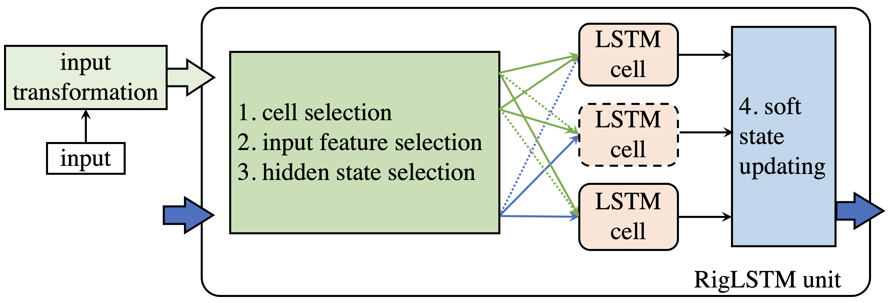
Figure 1: An illustration of the unit of recurrent independent Grid LSTM (RigLSTM). The RigLSTM contains multiple LSTM cells, and four steps are performed at each time step inside the unit, i.e., cell selection, input feature selection, hidden state selection and soft state updating.

In this paper, based on the above observations on RIM, a novel recurrent unit called recurrent independent Grid LSTM (RigLSTM) is proposed, which is illustrated in Fig. 1, aiming at facilitating uncovering and exploiting the modular structures for sequence modeling tasks with environment changes during testing. In the RigLSTM unit, we propose cell selection, input feature selection, hidden state selection, and soft state updating to overcome the concerns mentioned above. The RigLSTM unit contains multiple LSTM cells and each cell are expected to perform independently. At a certain time step, the input are first transformed into multiple feature vectors, which can be seen as features from multiple views. Different view can provide different information needed by the following steps. Then, the relevance scores between the input features and the hidden states are computed, based on which the cell selection step is performed. Only the activated cells can select relevant input features and hidden states of other cell as input to update their states independently. At last, the soft state updating is employed to facilitate information flow from previous time step to the current time step. Experiments are conducted on multiple sequence modeling tasks across different domains to show that our model has a stronger generalization ability when there exist changes between training and testing environments. The main contributions of the paper are summarized as follows:

• For generalizable sequence learning, we propose input feature selection, cell selection, and hidden state selection, integrated with Grid LSTM, to allow for modularization, and decomposition of the input sequence into different subsystems. The specialization and modularization factorize the model into a few simpler and meaningful elements, leading to a more robust system than a homogeneous system [17] and a more light-weighted model than a direct ensemble [18].

• To ease training for the setting with environment changes during testing, we proposed soft state updating to propagate information from previous time step. The proposed method considers the current inputs and the states of others cells, which is ignored in other methods.

• Extensive experiments are conducted on diversified tasks and domains to evaluate the promising generalization ability of our approach, which can serve as an enhanced building block for LSTM, at the cost of moderately prolonged inference time. The source code will be made publicly available at the link: https://github.com/ziyuwwang/rig-lstm.

The rest of the paper is organized as follows. Section 2 introduces the related work and our main approach is presented in Section 3. The extensive empirical studies across different tasks are given in Section 4 and Section 5 concludes this paper.

2 Related Work

Our work is related to the modularity of neural network, multiple components and information flow through time in the recurrent models. We will give a brief summarization of these related areas and discuss the relationships with our work.

2.1 Modularity in Neural Networks

A network can be designed to be composed of several modules, and each module perform a distinct function. Thus, the whole network can be seen as a combination of module with different specialisms.

In [19], the authors designed neural module networks for the visual question answering. Several types of module are proposed, and questions are decomposed into linguistic substructures, which are then used to dynamically instantiate the network. A routing mechanism was proposed in [20] for the setting of multi-task learning. A routing network consists of two components, a router and a set of function blocks. Given an input, the router selects a function block to apply and pass the output back to the router recursively. The whole network is trained with reinforcement learning. Thus, the routing network composes different function blocks for each input dynamically. Similarly, a modular network was proposed in [21]. The modular networks model the probability of the modular to be chosen, and the whole network is trained with generalized Viterbi EM, without any artificial regularization. In [22], the relationships between systematic generalization and the module layout were studied on a synthetic VQA dataset. And it was found that end-to-end training do not facilitate systematic generalization and explicit regularization are required.

Most of the above models do not consider multiple activation and relevant input selection at a certain time step. However, these are the considered in our model.

2.2 Recurrent Models with Multiple Components

For complex sequence modeling, many works focus on splitting the memory cell or the hidden state into sub-groups. In Clockwork RNN [23], the authors proposed to divide the hidden state into groups with equal size, which are then updated with different frequencies. The interactions between groups occur periodically. While IndRNN [24] treats each single element in the hidden state separately, and the elements are updated completely independently. Grid LSTM [25] uses multiple recurrent cells and arranges them in a multidimensional grid. Except for vectors and sequences, it can be even applied to higher dimensional data like images. To enlarge the capacity of recurrent memory, Neural Turing Machines (NTM) [26], Differential Neural Computers (DNC) [27], and the more recent Memory Networks (MN) [28, 29] consider introducing external memory modules, which supports reading and writing operations based on the attention mechanism. For an explicit separation of memories, the Relational Memory Core (RMC) [15] introduces a matrix version of memory that is able to incorporate new inputs through a self-attention mechanism. Recurrent Entity Networks (EntNet) [30] develops a dynamic version of external memory for characterizing a sequence in a non-parallel way.

Recently, Recurrent Independent Mechanisms (RIM) [16] employs multiple RNN cells in a single recurrent unit, and it adopts a competing strategy to activate the relevant cells and a communication mechanism to allow cell to know the states of other cells at each certain time step. The designs are also adopted and improved by following works. Bidirectional recurrent independent mechanisms (BRIM) [31] combines bottom-up and top-down signals dynamically using attention, which leads to reliable performance improvements. In [32], the authors combined meta-learning with modular structure, and showed that meta-learning the modular structure among tasks helps achieve faster adaptation in reinforcement learning.

In RIM, the inactivated cells are updated with default dynamics. The activated cells also communicate with each other to exchange useful information. However, the irrelevant inputs are also fed into the cells, which leads to bad effects in forming specializations. Moreover, the communication in RIM does not consider the transition dynamic of the individual cells. Our work will exploit cell selection, input feature selection, hidden state selection, soft state updating that integrated with Grid LSTM to overcome these drawbacks of RIM.

2.3 Recurrent Models with Information Flow through Time

To facilitate the training and improving the generalization ability, information from previous hidden states is exploited at the current time step in some specially designed models. Zoneout [33] randomly keeps some hidden units unchanged from a previous time step. By preserving some part of hidden units, the information is more easily propagated through time. The recurrent highway network (RHN) [34] introduces a gating function to combine the previous hidden state and the current hidden state, which helps propagate the gradient flow. Thus, the recurrent depth can be significantly increased in RHN. RIM [16] and RMC [15] exploit residual connections from previous hidden states to help propagate information through time.

In this paper, we propose a soft state updating mechanism to combine the hidden states from the previous time step and the current step, by considering the contents of the current input and the states of the other cells. Our method aims to propagate gradient information, and enhance specialization among the cells for the tasks existing environment changes during testing.

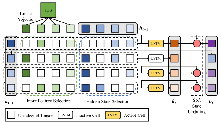
Figure 2: Recurrent Independent Grid LSTM (RigLSTM). The input is transformed to multiple tensors and selected by hidden states of each cell. Hidden vectors are selected by similar rules. The selected input and hidden vectors are concatenated and fed into LSTM cells. Only the LSTM cells with the highest sum of similarity scores with input vectors are activated, which are updated by the soft states updating mechanism. It combines newly computed hidden states with old ones.

3 Recurrent Independent Grid LSTM

In this section, we will give a brief introduction of Grid LSTM [25] as background. Then, we will present our model. Lastly, we will discuss the differences between our model and RIM.

3.1 Preliminaries on Grid LSTM

For an LSTM cell [35], the cell comprises a hidden vector $\bm{h}_{t-1}\in\mathbb{R}^{d}$ and a memory vector $\bm{c}_{t-1}\in\mathbb{R}^{d}$, where $d$ is the size of hidden state vector. Taking a vector $\bm{x}_{t}\in\mathbb{R}^{D}$ as input, where $D$ is the dimensionality of the input feature vector, the computation process inside an LSTM cell at time step $t$ is expressed as:

$$\bm{f}_{t} =\sigma(\bm{W}_{f}\bm{H}_{t}),$$ (1)

$$\bm{i}_{t} =\sigma(\bm{W}_{i}\bm{H}_{t}),$$ (2)

$$\bm{o}_{t} =\sigma(\bm{W}_{o}\bm{H}_{t}),$$ (3)

$$\bm{g}_{t} =\operatorname{tanh}(\bm{W}_{g}\bm{H}_{t}),$$ (4)

$$\bm{c}_{t} =\bm{f}_{t}\odot\bm{c}_{t-1}+\bm{i}_{t}\odot\bm{g}_{t},$$ (5)

$$\bm{h}_{t} =\bm{o}_{t}\odot\operatorname{tanh}(\bm{c}_{t}),$$ (6)

where $\sigma$ is the logistic sigmoid function and $\bm{W}_{f},\bm{W}_{i},\bm{W}_{o},\bm{W}_{g}\in\mathbb{R}^{(D+d)\times d}$ are all linear transformation matrices. $\bm{H}_{t}$ is the concatenation of the input $\bm{x}_{t}$ and the previous hidden vector $\bm{h}_{t-1}$, whihc can expressed as

$$\bm{H}_{t}=\left[\bm{x}_{t},\bm{h}_{t-1}\right],$$ (7)

where $[\cdot,\cdot]$ is the concatenation operator that stacks column vectors vertically to form a new column vector. The above process is denoted as:

$$\bm{h}_{t},\bm{c}_{t}=\operatorname{LSTM}\left(\bm{H}_{t},\bm{c}_{t-1};\bm{W}\right),$$ (8)

where $\bm{W}$ is the set of trainable parameters, i.e., $\bm{W}_{f},\bm{W}_{i},\bm{W}_{o}$ and $\bm{W}_{g}$.

Grid LSTM [25] is a recurrent unit that contains $N$ LSTM cells, and each cell update its own states individually. At time step $t$, we denote the hidden state vectors of the LSTM cells as $\bm{h}^{1}_{t},...,\bm{h}^{N}_{t}$, and memory vectors as $\bm{c}^{1}_{t},...,\bm{c}^{N}_{t}$. Given an input $\bm{x}_{t}$, the Grid LSTM is updated as

$$\bm{h}^{1}_{t},\bm{c}^{1}_{t} =\operatorname{LSTM}\left(\bm{H}_{t},\bm{c}^{1}_{t-1};\bm{W}^{1}\right),$$ (9)

$$\ ...,$$ (10)

$$\bm{h}^{N}_{t},\bm{c}^{N}_{t} =\operatorname{LSTM}\left(\bm{H}_{t},\bm{c}^{N}_{t-1};\bm{W}^{N}\right),$$ (11)

where $\bm{H}_{t}$ is defined as

$$\bm{H}_{t}=\left[\bm{x}_{t},\bm{h}^{1}_{t-1},\cdots,\bm{h}^{N}_{t-1}\right].$$ (12)

$\bm{W}^{k}$ is a collection of transformation matrices for the $k$-th LSTM cell. Each LSTM cell inside a Grid LSTM has distinct parameter matrices $\bm{W}^{k}_{f},\bm{W}^{k}_{i},\bm{W}^{k}_{o},\bm{W}^{k}_{g}$, and updates with individual dynamics. In this way, the Grid LSTM unit enables all internal LSTM cells to communicate with each other while operate independently.

3.2 Recurrent Independent Grid LSTM

The overall structure of our model is illustrated in Fig. 2. We can see that our model contains several LSTM cells, and each cell is designed to update with independent transition dynamics. At a certain time step, the input is firstly transformed into multiple vectors to provide different views for the cells, since each cell might need different aspects of the input. Then, a subset of cells are activated, and each activated cell selects transformed input features and relevant cell states as its inputs to update the state according its own transition dynamics. At last, to facilitate information flow through time, the soft updating is exploited.

The details about our model will be presented in the following subsections. To provide clear descriptions, the notations are summarized in the Table I.

TABLE I: A summery of notations used in the paper.

Notation	Meaning
$d$	The dimentionality of LSTM hidden states.
$N$	The number of LSTM cells in one unit.
$K$	The number of input feature vectors.
$K_{x}$	The number of selected input feature vectors.
$K_{h}$	The number of selected hidden state vectors.
$K_{a}$	The number of selected cells.
$S_{t}^{j}$	The set of top $K_{x}$ inputs.
$R_{t}^{j}$	The set of top $K_{h}$ hidden states.
$C_{t}^{j}$	The set of top $K_{a}$ cells selected.
$\mathbf{H}_{t}^{j}$	The input for the $j$-th LSTM cell at time step $t$.
$\mathbf{h}_{t}^{j}$	The hidden state of the $j$-th LSTM cell at time step $t$ after regular update.
$\tilde{\mathbf{h}}_{t}^{j}$	The hidden state of the $j$-th LSTM cell at time step $t$ after soft updating.
$\mathbf{h}_{t-1}^{k,j}$	The $k$-th input hidden state for the $j$-th LSTM cell at time step $t$ after hidden state selection.
$\mathbf{x}_{t}^{k,j}$	The $k$-th input for the $j$-th LSTM cell at time step $t$ after input selection.

3.2.1 Input Transformation

In our model, the cells are expected to be responsible for a certain aspect of the whole system. Thus, the inputs needed for each cell might be different. To facilitate each cell to form specialization, the input feature is transformed into multiple feature vectors with linear transformation to provide different views of the input for the cells. Ideally, each cell only absorbs information from the views needed. Specifically, the input $\bm{x}_{t}$ at time step $t$ is first transformed into $K$ vectors $\bm{x}^{1}_{t},\bm{x}^{2}_{t},...,\bm{x}^{K}_{t}\in\mathbb{R}^{d}$, which can be seen as multiple views of the input.

3.2.2 Cell Selection

A similarity score between the $k$-th input feature vector and the $j$-th LSTM cell is computed as:

$$s_{k,j}=\bm{x}^{k}_{t}\cdot\bm{h}^{j}_{t},$$ (13)

where $\cdot$ is the inner product between two vectors.

The proposed model is designed to dynamically select the LSTM cells that are relevant to the current input. For the $j$-th LSTM cell, the relevance score is computed as

$$s_{j}=\sum_{k}s_{k,j},$$ (14)

where $s_{k,j}$ is the score defined in Eq. (13). Thus, the relevance score is the sum of the scores between the $K$ inputs and the LSTM cell state. At each time step, the top $K_{a}$ cells are selected (activated), denoted by $C_{t}$. The hidden states of the selected LSTM cells are updated with the soft state updating, which will be described below. The hidden state vectors and memory vectors of the inactivated LSTM cells remain unchanged.

3.2.3 Input Feature Selection

At each time step, for the $j$-th LSTM cell, we select the top $K_{x}$ out of $K$ input features according to the similarity scores, and denote the collection of top $K_{x}$ inputs as set $S_{t}^{j}$. Then, the input feature vectors for $j$-th LSTM cell are determined by the rules:

$$\bm{x}^{k,j}_{t}=\begin{cases}\bm{x}^{k}_{t}&\bm{x}^{k}_{t}\in S_{t}^{j}\\ \bm{0}&\bm{x}^{k}_{t}\notin S_{t}^{j}.\end{cases}$$ (15)

The proposed input selection strategy is designed to enhance the diversity of each LSTM cell’s input. While the operation of replacing the unselected vectors with all-zeros is for more consistent modeling and easier optimization.

3.2.4 Hidden State Selection

Similar to the input feature vector selection, each LSTM cell also selects the hidden states of relevant cells as inputs, to obtain the information from related cells. The selection is based on the similarity between cells. Since the hidden state vectors have the same dimensionalities, we simply use the inner product between hidden states. For the $j$-th cell, its own hidden vector is to be selected. For the rest $(N-1)$ hidden states, we select the top $K_{h}$, denoted as $R_{t}^{j}$. For the $j$-th LSTM cell, we define

$$\bm{h}^{k,j}_{t-1}=\begin{cases}\bm{h}^{k}_{t-1}&\bm{h}^{k}_{t-1}\in R_{t}^{j}\ \text{or}\ k=j\\ \bm{0}&\bm{h}^{k}_{t-1}\notin R_{t}^{j}\end{cases}$$ (16)

and by combining with the input feature selection, we obtain the input vector $\bm{H}^{j}_{t}$ for the $j$-th LSTM cell:

$$\bm{H}^{j}_{t}=\left[\bm{x}^{1,j}_{t},\cdots,\bm{x}^{K,j}_{t},\bm{h}^{1,j}_{t-1},\cdots,\bm{h}^{N,j}_{t-1}\right].$$ (17)

3.2.5 Soft State Updating

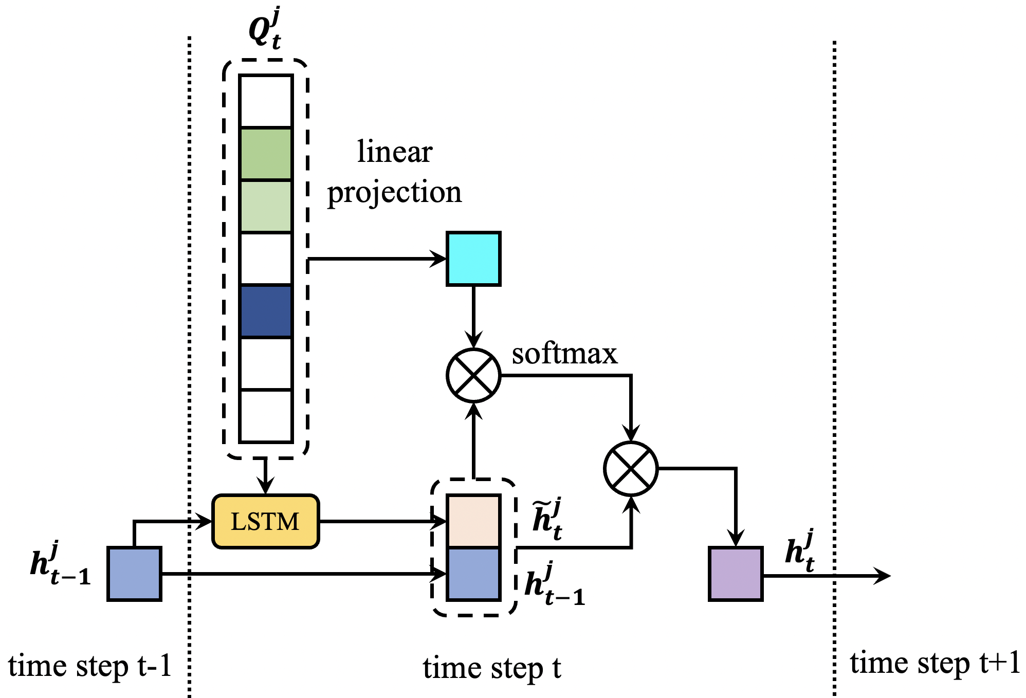
Figure 3: An illustration of the soft state updating mechanism proposed in this paper. For the $j$-th LSTM cell, all relevant inputs and selected hidden states, except its own hidden state, are concatenated into one vector. Then the weights for $\tilde{\bm{h}}^{j}_{t}$ and $\bm{h}^{j}_{t-1}$ are computed by considering the similarities between them. The final hidden state $\bm{h}^{j}_{t}$ is a weighted sum of $\tilde{\bm{h}}^{j}_{t}$ and $\bm{h}^{j}_{t-1}$.

To facilitate information propagation through time and to ease the training, we propose a soft state updating mechanism for activated cells, which is illustrated in Fig. 3.

For the $j$-th LSTM cell, after the regular hidden state update step, we can obtain the hidden states $\tilde{\bm{h}}_{t}$, which is expressed as:

$$\tilde{\bm{h}}^{j}_{t},\bm{c}^{j}_{t} =\operatorname{LSTM}\left(\bm{H}^{j}_{t},\bm{c}^{j}_{t-1};\bm{W}^{j}\right).$$ (18)

All the selected vectors of the $j$-th cell except for $\bm{h}^{j,j}_{t-1}$ are concatenated to form $\bm{Q}^{j}_{t}$, as given by:

$$\bm{Q}^{j}_{t}=\left[\bm{x}^{1,j}_{t},\cdots,\bm{x}^{K,j}_{t},\bm{h}^{1,j}_{t-1},\cdots,\bm{h}^{j-1,j}_{t-1},\bm{h}^{j+1,j}_{t-1},\cdots,\bm{h}^{N,j}_{t-1}\right].$$ (19)

Then, we stack the hidden states from the previous step and the current step to form a matrix

$$\bm{K}^{j}_{t}=\left[\bm{h}^{j}_{t-1};\tilde{\bm{h}}^{j}_{t}\right],$$ (20)

where $[\cdot;\cdot]$ is an operator for $n$ column vectors of size $d$ to form a $d\times n$ matrix. We express the final hidden state as

$$\bm{h}^{j}_{t}=\bm{K}^{j}_{t}\operatorname{softmax}\left(\left(\bm{K}^{j}_{t}\right)^{\top}\bm{W}_{q}\bm{Q}^{j}_{t}\right),$$ (21)

where $\bm{W}_{q}$ is linear transformation matrix. We can see that the combination weights for the previous states and current state are determined by the input feature vectors and the hidden state from all the cells. Thus, the information propagation through time in our model is effected by the context information, which will be showed to be effective for the setting of generalizable sequence learning.

3.3 Differences with RIM

RIM contains three steps, i.e., cell selection, independent hidden state updating and communication among hidden states. The relevant cells are activated by computing the similarity between the hidden states and the input. Only the cells of high similarity with the current input are activated. The activated cells update their state with independent transition dynamics. At last, the updated cells communicate with all the other cells via attention mechanism. We will discuss the differences between our model and RIM on the following aspects in detail.

3.3.1 On Inputs

The input of each LSTM cell in RIM is a weighted sum of an original input and a null input, implying that inputs of the LSTM cells are the same vector multiplied by different coefficients. Thus, the information fed into cells are the same. However, our RigLSTM removes the null input, and transforms the original input into multiple features vectors, each of which captures different information of the original input. Then, each cell selects relevant feature vectors by similarity between the transformed feature vectors and the corresponding hidden states. Therefore, the information fed into the cells in our model are all different. Such distinctness in input will facilitate the cells to form specialization.

3.3.2 On Retrieving Context Information From Other Cells

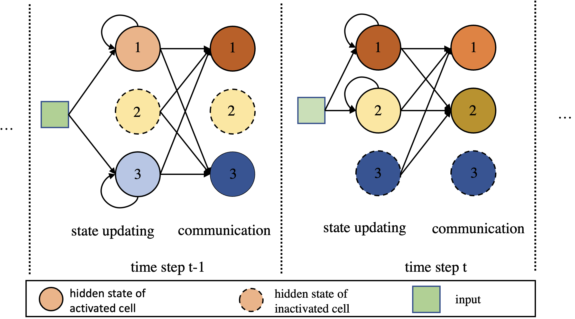
(a) An illustration of retrieving context information in the state updating in RIM. Cell 1 is activated at time step $t$ and $t-1$, and cell 2 is only activated at time step $t$. When performing state updating at time step $t$, cell 1 knows the state of other cells from the communication step performed at time step $t-1$. Cell 2 does not have the chance since it is not activate at time step $t-1$. Thus, the state updating step of cell 2 lacks updated context information. Thus, each cell might have outdated context information.

(b) An illustration of retrieve context information during state updating in the proposed RigLSTM. Each cell selects relevant hidden state of the other cells as input to perform state updating. Even if cell 2 is not activated at time step $t-1$, it still knows the updated state information from all the other cells. Thus, each cell has updated context information.

Figure 4: Comparisons of the ways how to retrieving context information from other cells when performing state updating steps in between RIM and RigLSTM.

The cells in the recurrent unit need to know the states of other cells, so as to cooperate with each other. In RIM, each activated cell performs communication step after updating their own state independently. The cells do not know the states of other cells when performing state updating. However, the state updating step and communication step are combined into one single step in our proposed unit. And the cells in our model update their states knowing the context information.

In RIM, a cell which is activated at the current time step but not activated at the previous time step will lack updated context information when performing state updating. An example is shown in Fig. 4(a). Cell-1 is activated at time step $t$ and $t-1$. Therefore, cell-1 have the context information from other cells implicitly at time step $t$, since the hidden state of cell-1 can retrieve necessary information via communication at time step $t-1$, which will be fed into cell-1 at time step $t$. However, cell-2 does not have a chance to retrieve such information. Cell-2 is only activated at time step $t$, and no retrieving (communication) operation is performed at time step $t-1$. The state of cell-2 is updated with outdated context information.

In RigLSTM, each activated cell selects hidden states from other cell as inputs. Thus, they all know the necessary context information. As shown in Fig. 4(b), cell-2 at the time step $t$ knows the states of cell-1 and cell-2. Therefore, the actions depending on the hidden state of cell-2 is more reliable. The effectiveness will be illustrated with experiments in the following section.

3.3.3 On Information propagation through Time

In RIM, for activated cells, the information of hidden state from previous time step is propagated to the current time step with residual connections. However, in our model, the soft state updating mechanism considers all relevant input features and hidden states from other cells to determine the combination coefficients. Thus, the inputs and the states of other cell can effect information flow through time for the activated cells. Such design can benefit the forming of specialization of the cells, which will be illustrated in the following section.

4 Experiments

We conduct experiments on both synthetic and real-world benchmarks to show the advantages of our models, especially the generalization ability when there exist some changes in testing environments.

4.1 Experimental Settings

The experiments are conducted on a single machine with 256G memory and 96 CPUs (Intel(R) Xeon(R) Platinum 8255C CPU @ 2.50GHz). The models trained with a single NVIDIA Tesla V100 GPU. Four representative tasks are used to compare the performances of competing models. For all the experiments, we use Adam as the optimizer and set the learning rate to 0.0001, if not otherwise specified.

4.2 Sequential Image Classification Task

In line with [25, 16], we consider the task of sending a sequence of pixels of an image into a recurrent model, and predicting its label. The generalization ability is evaluated on data with resolutions different from the training set. Experiments are designed based on the two well-know dataset: MNIST and CIFAR-10.

4.2.1 Experimental Settings

For MNIST, the resolution of training data is set to $14\times 14$, while the competing models are evaluated at three higher resolution settings ($16\times 16$, $19\times 19$, and $24\times 24$). For CIFAR-10, the resolution for training is $16\times 16$, and the resolutions for testing are $19\times 19$, $24\times 24$ and $32\times 32$. Images of various resolutions are obtained by performing a nearest-neighbour sampling method on original images. The images of MNIST [36] are converted into binary digits (0 or 1), and then embedded to dimension of 600. For the colorful images in CIFAR-10 [37], the three channels, of which pixel values are from 0 to 255, are separately embedded to dimension 200 and then concatenated to form the inputs. For RIM, the number of cells in one unit is set to 6. For RigLSTM, we set $K$ and $N$ to 6, and $K_{x}=K_{h}=K_{a}$. The dimensionalities of single cells are both set to 100. For fair comparisons, the LSTM model has a hidden size of 600. We use the same configuration for the other experiments if not otherwise specified.

TABLE II: Test accuracy ($\%$) on the sequential MNIST dataset. All models are trained on images with resolution $14\times 14$, and evaluated at three resolution settings. $N$ is the number of cell in one unit, and $K_{a}$ is the number of activated cell at a certain time step.

Models	($N,K_{a}$)	$16\times 16$	$19\times 19$	$24\times 24$
LSTM [35]	-	84.5	52.2	21.9
RIM [16]	(6, 4)	90.0	73.4	38.1
EntNet [30]	-	89.2	52.4	23.5
RMC [15]	-	89.58	54.23	27.75
Transformers [38]	-	91.2	51.6	22.9
GridLSTM [25]	-	88.32	38.1	20.84
BRIM [31]	-	88.6	74.2	51.4
RigLSTM	(6, 5)	89.50	80.71	59.60

4.2.2 Analysis

The experimental results of all models on MNIST dataset are presented in Table II. We can see that our model greatly improves the performance over the competing methods on most of the settings, especially when the changes on the testing environment are large. Note that almost all the models achieve the performance of about 90% for the $16\times$16 setting, which is a relative easy setting, because the changes between training and testing are small. For the other harder settings, our model achieved the best results. And the gaps between our model and all the other models are quite large. The reuslts on CIFAR-10 are shown in Table III. Similar phenonimenon can also be observed as on MNIST dataset. Thus, our model has the best generalization ability for the setting with environment changes.

We list three examples of cell selection results during testing in Fig 5. And the corresponding input feature selection scores and hidden state selection scores at the $289$-th time step are shown in Fig. 6. From Fig 5, it can be seen that the $5$-th cell (cell-4) is activated mostly on the pixels corresponding to stroke of digit, while the $1$-st cell (cell-0) is activated in the opposite way. It seems that cell-4 is responsible for capturing digit strokes and cell-0 is responsible for capturing the background. This confirms our hypothesis that each LSTM cell in RigLSTM is responsible for different functions and the whole network is well modularized. From Fig. 6, we can see that the similarity scores are quite diverse. The similarity pattern between inputs and cells is more stable than that between hidden states. For example, cell-1 favours the input-4, and cell-4 dislike input-2. The relationship between cells are more complex. It is natural because the inputs from different views provide quite different information, and different cells might need information from a certain view through all time steps. Moreover, the states of cells are effected by the inputs. It is not easy to form a stable relationships between cells. Results in Tables II and III and Figures 6 and  5 indicate that our design helps the cells form specializations, thus our model improve the generalization performance compared with other methods.

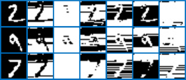
Figure 5: Examples of cells activation patterns when testing three digit images with resolution $24\times 24$ on MNIST dataset. The first column is the digit images, whose pixels are fed into models in the scan line order. Columns $2$ to $7$ show the activation image of 6 LSTM cells, respectively. A white pixel indicates that the LSTM cell is activated at the corresponding time step, while a black pixel indicates not activated.

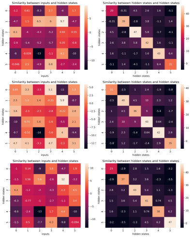
Figure 6: Examples of input selection scores (left column) and hidden state selection scores (right column). The pairs of scores are from the $289$-th time step of the three cases in Fig. 5.

TABLE III: Testing accuracy ($\%$) on sequential CIFAR-10 dataset. All models are trained on resolution $16\times 16$ and evaluated at 3 larger resolutions. $N$ is the number of cell in one unit, and $K_{a}$ is the number of activated cell at a certain time step.

Models	($N,K_{a}$)	$19\times 19$	$24\times 24$	$32\times 32$
LSTM [35]	-	54.4	44.0	32.2
RIM [16]	(6, 4)	56.9	51.4	40.1
RMC [15]	-	49.9	44.3	31.3
Transformers [38]	-	58.5	50.4	43.6
GridLSTM [38]	-	56.6	46.4	35.3
BRIM [31]	-	60.1	57.7	52.2
RigLSTM	(6, 4)	60.5	59.5	54.9

4.2.3 Ablation Study

TABLE IV: Ablation studies on sequential MNIST dataset. Top-1 classification accuracy (%) of variants of RigLSTM are reported.

Models	$16\times 16$	$19\times 19$	$24\times 24$
RigLSTM	89.50	80.71	59.60
$\text{RigLSTM}_{{no}\_{input}\_{trans}}$	86.32	55.28	35.75
$\text{RigLSTM}_{all\_cells}$	91.07	77.13	54.01
$\text{RigLSTM}_{rand\_cells}$	84.13	73.27	50.39
$\text{RigLSTM}_{all\_inputs}$	85.48	71.43	50.61
$\text{RigLSTM}_{rand\_inputs}$	83.5	70.26	48.84
$\text{RigLSTM}_{soft\_inputs}$	86.74	73.29	53.97
$\text{RigLSTM}_{all\_h}$	84.73	71.2	49.71
$\text{RigLSTM}_{rand\_h}$	85.24	73.56	48.35
$\text{RigLSTM}_{soft\_h}$	87.35	74.83	51.38
$\text{RigLSTM}_{no\_soft\_state\_updating}$	90.34	75.86	54.44

We also conduct ablation studies on the sequential MNIST dataset to analyze the effects of input transformation, input feature selection, hidden state selection, cell selection, and soft state update. We revise our model by changing or removing one component at a time to obtain a new model, and test the performance of the new model. The input feature selection and hidden state selection method in our model is a kind of hard selection method, i.e., a candidate of input feature or hidden states can only be selected of unselectied. To verify the necessarity, we design variants that select all input feature or hidden state, or soft selection, i.e., weighting the candidates with normalized scores. The details of these variants are described as follows:

• $\text{RigLSTM}_{{no}\_{input}\_{trans}}$: The input transformation step is removed, and the original input is fed into all the cells.

• $\text{RigLSTM}_{all\_cells}$: All cells are activated.

• $\text{RigLSTM}_{rand\_cells}$: $K_{a}$ cells are randomly activated.

• $\text{RigLSTM}_{all\_inputs}$: All inputs are selected for each LSTM cell.

• $\text{RigLSTM}_{rand\_inputs}$: $K_{x}$ input features are randomly selected for each LSTM.

• $\text{RigLSTM}_{soft\_inputs}$: Select all inputs, and each is weighted by the similarity scores normalized with softmax operation.

• $\text{RigLSTM}_{all\_h}$: All hidden states are selected for each LSTM.

• $\text{RigLSTM}_{rand\_h}$: $K_{h}$ hidden states are randomly selected for the LSTM cells.

• $\text{RigLSTM}_{soft\_h}$: Select all hidden states, and each of them is weighted with similarity scores normalized with softmax operation.

• $\text{RigLSTM}_{no\_soft\_state\_updating}$: Remove the soft state updating step. The hidden state at the end of time step $t$ for the $j$-th cell is $\tilde{\bm{h}}^{j}_{t}$.

The performances of the above models are shown in Table IV. We can see removing or changing any components will achieve worse performance. Thus, all the components, i.e., input transformation, cell selection, input feature selection, hidden state selection and soft state updating are all necessary for the RigLSTM model. The variants with random selection achieve almost the worse performances. It is natural that since it is not possible for the model to determine which input feature or cells will be fed into the model at each time step. Moreover, soft selection method is better than all selection method. For example, the performances on the three test setting of $\text{RigLSTM}_{soft\_h}$ are better than $\text{RigLSTM}_{all\_h}$, and $\text{RigLSTM}_{soft\_inputs}$ is also better than $\text{RigLSTM}_{all\_inputs}$. Thus, selecting relevant information is necessary for the setting existing environment changes when testing. And hard selection is better than soft selection. At last, we can see that our proposed soft state updating mechanism also improve the generalization performance, by comparing $\text{RigLSTM}_{no\_soft\_state\_updating}$ and RigLSTM. The reason might be that the combination of current state and previous states are determined by all the relevant information, including input features, hidden state of other cells. Such design helps the cells to know the context, thus improves the generalization ability.

4.2.4 Complexity Analysis

In this subsection, we compare the inference speed, number of parameters, GPU memory occupation of RigLSTM, LSTM and RIM. For fairness, the same sizes of hidden state are used, and the metrics are obtained on the the sequential MNIST dataset. The results are shown in Table V. We can see that the number of parameters of our model is a little larger than the others, which is mainly due to the increase of input dimensionality in each LSTM cell. For GPU memory usage, our model is better than RIM because the input selection and hidden state selection of LSTM cells are performed sequentially in our implementation, not in an parallel way. This leads to the extension of inference time. We implement RigLSTM in a very straightforward way for easy code reading and modifying, and the inference speed can be improved by more efficient implementations. Overall, RigLSTM trades a small increase in complexity for a significant performance improvement.

TABLE V: Inference time (ms), number of parameters and GPU memory occupation of different models tested on the sequential MNIST dataset. The batch size is 64.

Models	${(N,K_{a})}$	Inference Time			#Para	Memory
		$19\times 19$	$24\times 24$	$32\times 32$
LSTM [35]	-	66.4	93.5	149.1	2.8M	1621M
RIM [16]	(6, 4)	661.2	945.5	1502.4	3.0M	2604M
RigLSTM	(6, 4)	1133.2	1590.4	2550.2	3.6M	1915M

4.3 Bouncing Ball Video Prediction Task

Similar to previous works [16, 39], we evaluate our model by a synthetic “bouncing balls” task, in which multiple balls of different sizes and masses move with an initial setting of velocities. These balls are in motion under the basic laws of Newtonian Dynamics, where each ball will either keep the original movement state or change the state when a collision with the wall or other balls occurs.

4.3.1 Task Description

At each time step, the input is a 64$\times$64 image frame that indicates the current states of the balls. And each pixel is a 0-1 integer scalar, where one indicates that the pixel is part of a ball, and otherwise zero. The task is similar to video prediction, where we aim at predicting the next frame given previous ones. We utilize a CNN-based encoder and decoder for input feature extraction and output frame generation, respectively, in which the details of the encoder and decoder are exactly the same as those used in [39]. Finally, the binary cross-entropy (BCE) loss between predicted and ground-truth frames is adopted for optimization and evaluation.

4.3.2 Experimental Setting

We adopt LSTM [35], GridLSTM [25], Recurrent Independent Mechanisms (RIM) [16], and Recurrent Entity Networks (EntNet) [30] as the baseline models in our experiment. As the authors of RIM did not provide source code for this task, we conduct all the experiments based on our own implementation. Thus, we achieve the best performance of baseline RIM with hyper-parameters different from RIM paper. The dimensionality of input for all recurrent models is 512, and that of hidden state for LSTM is 250. The number of cells for EntNet, RIM, GridLSTM and RigLSTM is 5, with the individual hidden size of 50. There are three datasets of different numbers of balls and settings, abbreviated as 4 balls, 6-8 balls, and curtain, respectively. In specific, in 4 balls dataset, there are four balls moving and colliding during the whole process, while in 6-8 balls dataset the number could vary from 6 to 8. In the curtain dataset, a random rectangular curtain is applied to three moving balls in each frame during the time steps, which may occlude some certain balls at specified time steps. Such a dataset with occlusion is utilized to evaluate the transfer or generalization capability of the models. In each dataset, we have 50,000 sequences for training, and 10,000 sequences each for validation and testing, where each sequence contains 51 time steps of frames. We use learning rate 0.0003 to train each model until convergence (i.e., the validation loss does not decrease in 5 consecutive epochs). For testing, we feed the first 15 frames to generate 10 frames, and evaluate the performance with the loss on these 10 frames.

4.3.3 Analysis

We report the best test BCE loss in 5 runs on different datasets in Table VI: models with multiple cells are usually better than model with only one cell. Thus, employing multiple cells in one unit is necessary for the robustness to the changes in the testing environment. Moreover, our model achieves the best performance in most of the settings, which suggests that the advantages of our novel recurrent unit. To better understand how our model outperforms RIM, we visualize a sample in Fig. 7, which contains 10 frames of ground-truth and predicted results after feeding 15 frames into the models. We compare the predicted frames from RigLSTM (green), RIM (blue) to the ground-truth (pink balls) and see which model gives prediction closer to the ground-truth. As we can see, both RigLSTM’s and RIM’s results move slower than the ground truth, but RigLSTM’s balls can catch up faster comparing to the RIM baseline. Also, the results of RigLSTM are more like balls comparing to some oval-shaped results of RIM.

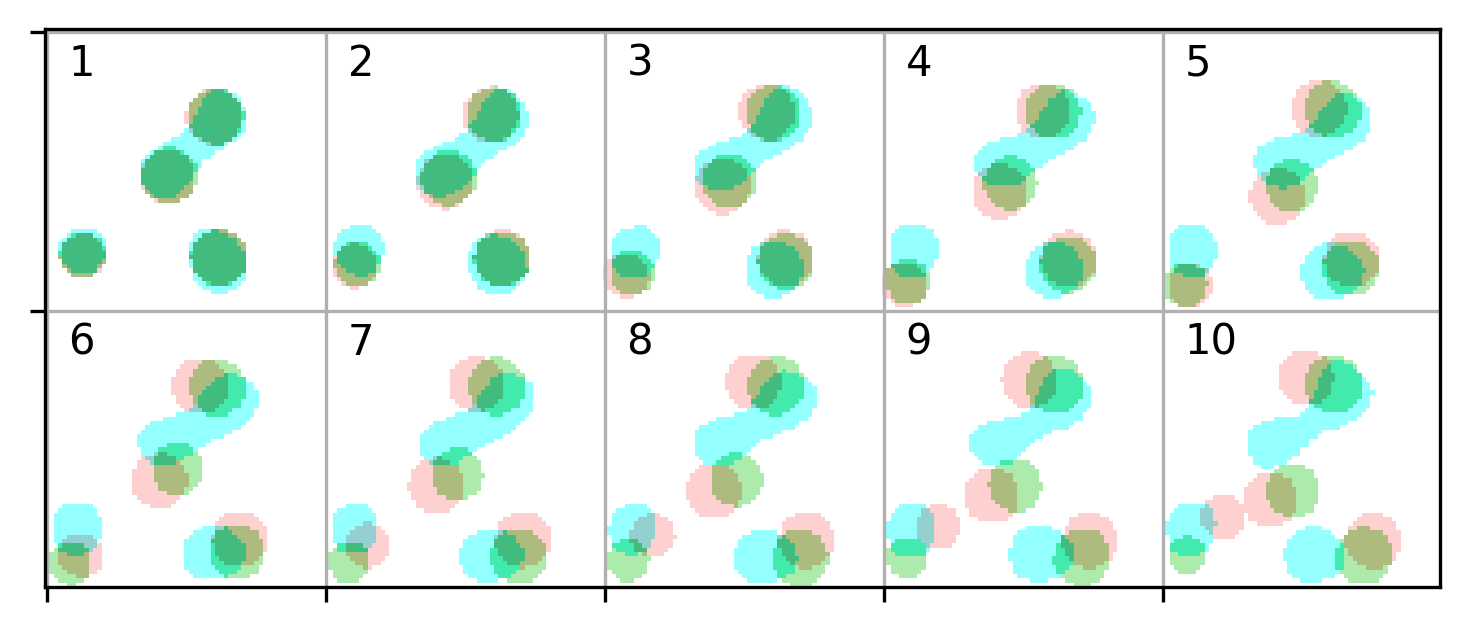
(a) Train on 4 and test on 4.

(b) Train on 4 and test on 678.

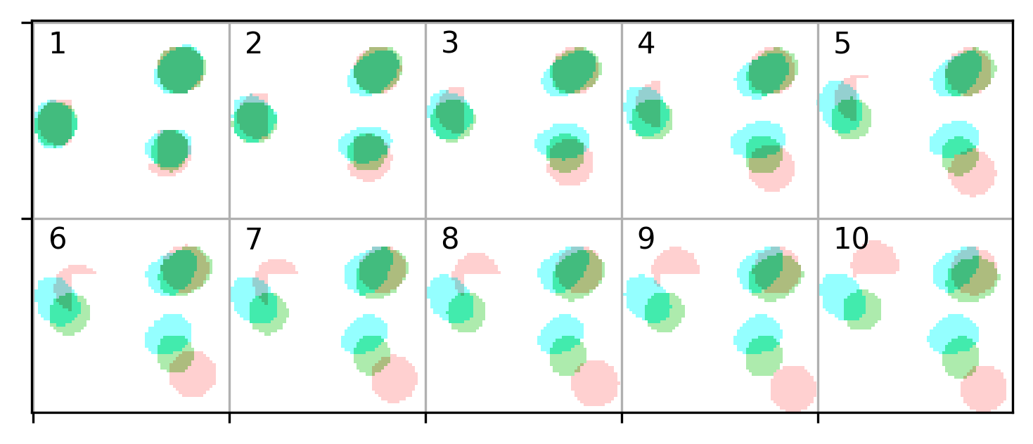
(c) Train on 4 and test with curtain.

Figure 7: Evaluation of RigLSTM and RIM on the Bouncing Ball experiments. The pink, green and blue balls denote predictions of ground-truth, RigLSTM and RIM, respectively.

TABLE VI: Roll-out BCE error (%) of bouncing-balls video prediction. We train each model on 4 balls and 6-8 balls datasets, and evaluate both in-distribution and out-of-distribution performances. Bold denotes the best on each task. For RIM [16] and RigLSTM [25], we set $N=5$, $K_{a}=2$ for the total number of cells and number of activated cells, respectively.

Training	4 balls			6-8 balls
Testing	4 ball	6-8 ball	curtain	6-8 ball	4 ball	curtain
RIM [16]	32.37	57.11	34.81	32.64	44.29	33.71
EntNet [30]	35.37	66.63	36.76	34.91	53.99	41.76
LSTM [35]	39.23	72.76	43.99	28.79	54.53	51.73
GridLSTM [25]	38.36	72.02	43.22	37.36	58.1	47.45
RigLSTM	30.52	49.19	31.72	31.53	42.64	33.51

4.4 Reinforcement Learning on MiniGrid

To evaluate our model on more complex problems, we conduct experiments on reinforcement learning (RL), in which the inputs and the environments are often complicated and challenging.

4.4.1 Task Description

Our experiments are conducted on OpenAI Gym-Minigrid, the world of which is an N$\times$M grid of tiles. Each tile can only contain one object, where an agent could take some certain actions at each time step, e.g., turn left, turn right, move forward, pick up, drop off, etc. For example, in a Door Key environment, an agent needs to pick up a key and and carries it to open the locked door in order to finish the game. In MiniGrid, there are many other environments for training an agent to take actions to accomplish such simple tasks. Therefore, it is a suitable platform to evaluate RigLSTM’s ability of learning a policy in various environments. In order to use reinforcement learning algorithms to guide the agent, we need first to define a reward for it. Note that given a time step $t$, the current situation is binary, i.e., job finished or not. We can give the agent a reward of one if it accomplishes the task within $F_{max}$ frames, otherwise, the reward is zero. In this way, the averaged reward can also be viewed as the success rate of the task.

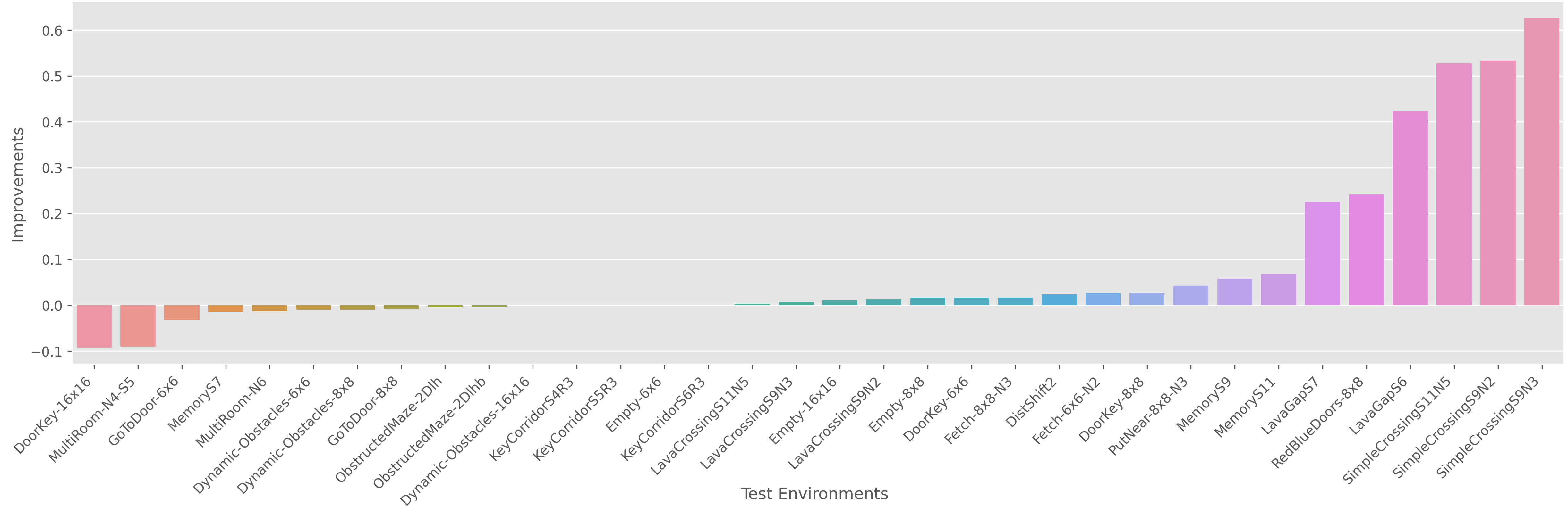
Figure 8: Relative value of rewards of RigLSTM-PPO over RIM-PPO on different tasks in MiniGrid. The mean of three trials is reported for fair comparison.

4.4.2 Experimental Settings

Experiments of this task are also conducted on our own implementation since no source code provided from the authors of RIM. We train our model and RIM [16] across all MiniGrid environments that have different levels of difficulty. All of the models are trained by Proximal Policy Optimization (PPO) [40]. To compare the generalization ability, we train them on the easiest environment and test their performance in all difficulty levels of that game, and then compare the mean rewards. For example, DoorKey environment has four difficulty levels, $5\times 5$, $6\times 6$, $8\times 8$, $16\times 16$. We only train the model on DoorKey-$5\times 5$ environment and test it on all of the four environments. To alleviate the effect of randomness, we conduct the experiments for each model-environment pair for three times with different random seeds and compare the mean rewards. We compare our RigLSTM based PPO (RigLSTM-PPO) with RIM based PPO (RIM-PPO). We use hyper-parameters ($N=4,K_{a}=2$) that perform best in most of the experiments conducted by the original RIM implementation for RIM-PPO, and ($N=4,K_{a}=4,K_{x}=4,K_{h}=4$) for RigLSTM-PPO, while all the other hyperparameters are the same for both models.

4.4.3 Analysis

The final results are shown in Fig. 8. The values in the figure are improvements on rewards comparing to that of RIM-PPO. We can see that using our RigLSTM in PPO can significantly increase the rewards the agents can get on most environments. For example, RigLSTM has the highest improvements in the SimpleCrossing environment, where the agent needs to cross many walls to reach the target point. Comparing to other game settings, small SimpleCrossing environment is generalized to larger environments in the way that the agent only needs to notice where the target is and then moves towards it by avoiding walls. In such a situation, the superiority of the input and hidden states selection mechanism of RigLSTM can greatly help the agent identify its current state and move to the target faster. Thus, RigLSTM often outperforms RIM in this environment.

4.5 Experiments on Multi-digit Copying Task

Digits memorization tasks are widely utilized in evaluating the abilities of recurrent neural networks. Typical memorization tasks, such as the copying task, usually require recurrent models to reproduce the given sequence after receiving a long sequence of blanks to evaluate if a model is able to memorize the input digit sequence. We aim at evaluating the generalization ability when existing environment changes and robustness against complex inputs. And we design a new task for such a purpose.

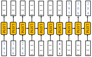
Figure 9: A simple example of 3-digit Copying Task, with $L=3$, $P=3$. At every time step before the dormant phase, 3 digits are fed into the recurrent models. Once the model receive the special token, it starts to produce the output sequence. The accuracy is computed based on the generated sequence.

4.5.1 Task Description

Our task is to memorize a multi-digit sequence. In this new task, the input at each time step is no longer a single digit, but $M$ digits. The model receives a sequence of multi-digit followed by a sequence of blanks, called dormant phase. Then, the model needs to reproduce the input sequence. The goal of models is to reproduce the input sequence. Formally, the input sequence is denoted as $A=\{\bm{a}_{1},\bm{a}_{2},\cdots,\bm{a}_{L}\}$, where $\bm{a}_{i}$ is the input at the $i$-th time step and $\bm{a}_{i}$ is a sequence of $M$ digits. The dormant phase is a sequence of blanks of length $P$. A special token is fed into the model after the $M$-digit sequence and dormant phase as a sign for model to produce the output sequence. An example is illustrated in Fig. 9.

TABLE VII: Testing accuracy ($\%$) on Multi-digit Copying Task. Models are trained with dormant length 50 and evaluated in three dormant length settings ($P=100,200,400$) respectively.

Models	($N,K_{a}$)	$M$	Test Acc ($P=100$)	Test Acc ($P=200$)	Test Acc ($P=400$)
LSTM [35]	-	1	45.38	25.19	16.09
GridLSTM [25]	-	1	50.26	28.43	20.36
RIM [16]	(6, 4)	1	97.75	95.14	84.85
RigLSTM	(6, 4)	1	99.06	98.89	97.66
LSTM [35]	-	2	29.74	11.51	10.70
GridLSTM [25]	-	2	31.25	15.37	14.26
RIM [16]	(6, 4)	2	94.45	89.30	79.59
RigLSTM	(6, 4)	2	98.28	95.43	92.63
LSTM [35]	-	4	25.07	12.81	10.06
GridLSTM [25]	-	4	29.33	15.94	12.11
RIM	(6, 4)	4	75.91	70.80	63.23
RigLSTM	(6, 4)	4	95.61	92.46	89.95
LSTM [35]	-	8	18.52	11.74	10.07
GridLSTM [25]	-	8	21.25	14.09	12.75
RIM [16]	(6, 4)	8	65.46	52.26	42.27
RigLSTM	(6, 4)	8	90.24	87.95	84.59

4.5.2 Experimental Settings

For generalization ability testing, the recurrent models are trained with dormant phase length setting to 50, and evaluated with dormant phase lengths equal to 100, 200 and 400. We set $M$ with varying values, i.e, $1,2,4$ and $8$, to evaluate their abilities when the task becomes difficult. The sequence length $L$ is fixed to 10, and all digits are randomly sampled from $[0,9]$. We take LSTM and RIM as our baseline models, and compare them with our model in terms of testing accuracy.

4.5.3 Analysis and Discussion

The results are shown in Table VII. We can see that our model achieves the best performance under all the settings. For most cases, the performances of LSTM and GridLSTM are rather poor, which proves that special designs are necessary for the testing cases when environment changes. When $M$ is small, e.g., 1 and 2, the task is relatively easy. Both RIM and RigLSTM provide satisfying generalization abilities. However, when the task becomes harder, our model is far better than RIM and the gap also become larger. Thus, RigLSTM performs significantly better than RIM for complex inputs. This might be attributed to the input selection and hidden state design, which makes the cells in our model better at selecting relevant information as inputs. Moreover, as the length of dormant length becomes larger, the performance of all models drops. But RigLSTM can still achieve accuracy $84\%$ for the test with dormant phase length set to 400 and $M=8$, while the accuracy of RIM is only $42\%$. It suggests that RigLSTM is more robust to the changes of dormant phase length. This superiority of our model in the generalization ability may be due to the soft state updating mechanism. Compared with RIM, our state updating design is more effective for propagation of information from previous states. Overall, the designs of cell selection, input transformation and feature selection, hidden state selection and soft state updating greatly improve the generalization ability when environment changes, and help our model achieve far better performance than RIM.

5 Conclusion

We have proposed the recurrent independent Grid LSTM (RigLSTM) for generalizable sequence learning. It aims to decouple and streamline the modeling of underlying modular subsystems with sparse interaction over time. RigLSTM is composed of a group of independent LSTM cells that can actively cooperate with each other. We proposed cell selection, input selection, hidden state selection, and soft state updating, integrated with the Grid LSTM, to exploit the underlying modular structures on sequence modeling tasks. The cell selection forces the cells inside the proposed unit to form specialisms. The input selection helps the LSTM cells to select only relevant input information, the hidden state selection facilitate the LSTM cells to absorb only relevant context information. By virtue of the proposed components, our model enjoys competitive generalization and robustness, which has been validated on diversified sequence modeling tasks. The source code will be made publicly available.

References

- [1] J. L. Elman, “Finding structure in time,” Cognitive Science, vol. 14, no. 2, pp. 179–211, 1990.
- [2] T. Mikolov, M. Karafiát, L. Burget, J. Černockỳ, and S. Khudanpur, “Recurrent neural network based language model,” in InterSpeech, 2010.
- [3] O. Vinyals, A. Toshev, S. Bengio, and D. Erhan, “Show and tell: A neural image caption generator,” in Proceedings of the IEEE conference on computer vision and pattern recognition, 2015, pp. 3156–3164.
- [4] K. Xu, J. Ba, R. Kiros, K. Cho, A. Courville, R. Salakhudinov, R. Zemel, and Y. Bengio, “Show, attend and tell: Neural image caption generation with visual attention,” in International conference on machine learning, 2015, pp. 2048–2057.
- [5] S. Venugopalan, M. Rohrbach, J. Donahue, R. Mooney, T. Darrell, and K. Saenko, “Sequence to sequence-video to text,” in international conference on computer vision, 2015, pp. 4534–4542.
- [6] R. Krishna, K. Hata, F. Ren, L. Fei-Fei, and J. Carlos Niebles, “Dense-captioning events in videos,” in International conference on computer vision, 2017, pp. 706–715.
- [7] H. Mei and J. M. Eisner, “The neural hawkes process: A neurally self-modulating multivariate point process,” in NeurIPS, 2017, pp. 6754–6764.
- [8] S. Xiao, M. Farajtabar, X. Ye, J. Yan, L. Song, and H. Zha, “Wasserstein learning of deep generative point process models,” in NeurIPS, 2017, pp. 3247–3257.
- [9] M. Babaeizadeh, C. Finn, D. Erhan, R. H. Campbell, and S. Levine, “Stochastic variational video prediction,” in International Conference on Learning Representations, 2018.
- [10] E. Denton and R. Fergus, “Stochastic video generation with a learned prior,” in ICML, 2018, pp. 1182–1191.
- [11] M. J. Hausknecht and P. Stone, “Deep recurrent q-learning for partially observable mdps,” in AAAI, 2015, pp. 29–37.
- [12] I. Sorokin, A. Seleznev, M. Pavlov, A. Fedorov, and A. Ignateva, “Deep attention recurrent q-network,” arXiv preprint arXiv:1512.01693, 2015.
- [13] J. Chung, C. Gulcehre, K. Cho, and Y. Bengio, “Empirical evaluation of gated recurrent neural networks on sequence modeling,” arXiv preprint arXiv:1412.3555, 2014.
- [14] S. Hochreiter and J. Schmidhuber, “Long short-term memory,” Neural computation, vol. 9, no. 8, pp. 1735–1780, 1997.
- [15] A. Santoro, R. Faulkner, D. Raposo, J. W. Rae, M. Chrzanowski, T. Weber, D. Wierstra, O. Vinyals, R. Pascanu, and T. P. Lillicrap, “Relational recurrent neural networks,” in NeurIPS, 2018, pp. 7310–7321.
- [16] A. Goyal, A. Lamb, J. Hoffmann, S. Sodhani, S. Levine, Y. Bengio, and B. Schölkopf, “Recurrent independent mechanisms,” arXiv preprint arXiv:1909.10893, 2019.
- [17] J. Schmidhuber, “One big net for everything,” arXiv preprint arXiv:1802.08864, 2018.
- [18] S. Zhang, M. Liu, and J. Yan, “The diversified ensemble neural network,” Advances in Neural Information Processing Systems, vol. 33, 2020.
- [19] J. Andreas, M. Rohrbach, T. Darrell, and D. Klein, “Neural module networks,” in Conference on Computer Vision and Pattern Recognition, 2016, pp. 39–48.
- [20] C. Rosenbaum, T. Klinger, and M. Riemer, “Routing networks: Adaptive selection of non-linear functions for multi-task learning,” arXiv preprint arXiv:1711.01239, 2017.
- [21] L. Kirsch, J. Kunze, and D. Barber, “Modular networks: Learning to decompose neural computation,” Advances in neural information processing systems, vol. 31, 2018.
- [22] D. Bahdanau, S. Murty, M. Noukhovitch, T. H. Nguyen, H. de Vries, and A. Courville, “Systematic generalization: what is required and can it be learned?” arXiv preprint arXiv:1811.12889, 2018.
- [23] J. Koutnik, K. Greff, F. Gomez, and J. Schmidhuber, “A clockwork rnn,” in International Conference on Machine Learning, 2014, pp. 1863–1871.
- [24] S. Li, W. Li, C. Cook, C. Zhu, and Y. Gao, “Independently recurrent neural network (indrnn): Building a longer and deeper rnn,” in Conference on Computer Vision and Pattern Recognition, 2018, pp. 5457–5466.
- [25] N. Kalchbrenner, I. Danihelka, and A. Graves, “Grid long short-term memory,” arXiv preprint arXiv:1507.01526, 2015.
- [26] A. Graves, G. Wayne, and I. Danihelka, “Neural turing machines,” arXiv preprint arXiv:1410.5401, 2014.
- [27] A. Graves, G. Wayne, M. Reynolds, T. Harley, I. Danihelka, A. Grabska-Barwińska, S. G. Colmenarejo, E. Grefenstette, T. Ramalho, J. Agapiou et al., “Hybrid computing using a neural network with dynamic external memory,” Nature, vol. 538, no. 7626, pp. 471–476, 2016.
- [28] J. Weston, S. Chopra, and A. Bordes, “Memory networks,” in ICLR, 2015.
- [29] S. Sukhbaatar, A. Szlam, J. Weston, and R. Fergus, “End-to-end memory networks,” in NeurIPS, 2015, pp. 2440–2448.
- [30] M. Henaff, J. Weston, A. Szlam, A. Bordes, and Y. LeCun, “Tracking the world state with recurrent entity networks,” in International Conference on Learning Representations, 2017.
- [31] S. Mittal, A. Lamb, A. Goyal, V. Voleti, M. Shanahan, G. Lajoie, M. Mozer, and Y. Bengio, “Learning to combine top-down and bottom-up signals in recurrent neural networks with attention over modules,” in International Conference on Machine Learning, 2020, pp. 6972–6986.
- [32] K. Madan, R. N. Ke, A. Goyal, B. B. Schölkopf, and Y. Bengio, “Fast and slow learning of recurrent independent mechanisms,” arXiv preprint arXiv:2105.08710, 2021.
- [33] D. Krueger, T. Maharaj, J. Kramár, M. Pezeshki, N. Ballas, N. R. Ke, A. Goyal, Y. Bengio, A. Courville, and C. Pal, “Zoneout: Regularizing rnns by randomly preserving hidden activations,” arXiv preprint arXiv:1606.01305, 2016.
- [34] J. G. Zilly, R. K. Srivastava, J. Koutnık, and J. Schmidhuber, “Recurrent highway networks,” in International Conference on Machine Learning, 2017, pp. 4189–4198.
- [35] S. Hochreiter and J. Schmidhuber, “Long short-term memory,” Neural Computation, vol. 9, no. 8, pp. 1735–1780, 1997.
- [36] Y. LeCun, L. Bottou, Y. Bengio, and P. Haffner, “Gradient-based learning applied to document recognition,” Proceedings of the IEEE, vol. 86, no. 11, pp. 2278–2324, 1998.
- [37] A. Krizhevsky, G. Hinton et al., “Learning multiple layers of features from tiny images,” Tech Report, 2009.
- [38] A. Vaswani, N. Shazeer, N. Parmar, J. Uszkoreit, L. Jones, A. N. Gomez, L. Kaiser, and I. Polosukhin, “Attention is all you need,” in NeurIPS, 2017, pp. 5998–6008.
- [39] S. van Steenkiste, M. Chang, K. Greff, and J. Schmidhuber, “Relational neural expectation maximization: Unsupervised discovery of objects and their interactions,” in ICLR, 2018.
- [40] J. Schulman, F. Wolski, P. Dhariwal, A. Radford, and O. Klimov, “Proximal policy optimization algorithms,” arXiv preprint arXiv:1707.06347, 2017.