Towards objective and systematic evaluation of bias in medical imaging AI

Abstract

Background. Artificial intelligence (AI) models trained using medical images for clinical tasks often exhibit bias in the form of disparities in performance between subgroups. Since not all sources of biases in real-world medical imaging data are easily identifiable, it is challenging to comprehensively assess how those biases are encoded in models, and how capable bias mitigation methods are at ameliorating performance disparities. In this article, we introduce a novel analysis framework for systematically and objectively investigating the impact of biases in medical images on AI models.

Methods. We developed and tested a framework for conducting controlled in silico trials to assess bias in medical imaging AI using a tool for generating synthetic magnetic resonance images with known disease effects and sources of bias. The feasibility of this framework is showcased by using three counterfactual bias scenarios to measure the impact of simulated bias effects on a convolutional neural network (CNN) classifier and the efficacy of three bias mitigation strategies.

Findings. The analysis revealed that the simulated biases resulted in expected subgroup performance disparities when the CNN was trained on the synthetic datasets. Moreover, reweighing was identified as the most successful bias mitigation strategy for this setup, and we demonstrated how explainable AI methods can aid in investigating the manifestation of bias in the model using this framework.

Interpretation. Developing fair AI models is a considerable challenge given that many and often unknown sources of biases can be present in medical imaging datasets. In this work, we present a novel methodology to objectively study the impact of biases and mitigation strategies on deep learning pipelines, which can support the development of clinical AI that is robust and responsible.

[label1]organization=Biomedical Engineering Graduate Program, University of Calgary,city=Calgary, country=Canada [label2]organization=Department of Radiology, University of Calgary,city=Calgary, country=Canada [label3]organization=Hotchkiss Brain Institute, University of Calgary,city=Calgary, country=Canada [label4]organization=Alberta Children’s Hospital Research Institute, University of Calgary,city=Calgary, country=Canada [label5]organization=Department of Electronics and Electrical Communication Engineering, Indian Institute of Technology,city=Kharagpur, country=India [label6]organization=Department of Pediatrics, University of Calgary,city=Calgary, country=Canada [label7]organization=Department of Community Health Sciences, University of Calgary,city=Calgary, country=Canada [label8]organization=Department of Clinical Neuroscience, University of Calgary,city=Calgary, country=Canada [label9]organization=Department of Electrical and Software Engineering, University of Calgary,city=Calgary, country=Canada

1 Introduction

Artificial intelligence (AI) systems are often praised for having the potential to serve as an objective decision-maker in health care. However, recent studies have shown that AI can produce systematic disparities in performance outcomes between subgroups; such models are considered to be biased or unfair. This is of particular concern in the domain of AI for medical imaging, where the first systems have been approved for assisting clinicians in making diagnostic and treatment decisions for their patients (Yearley et al., 2023). In this context, models may overfit to majority populations in the training data or learn spurious correlations that lead to poor generalization ability. For instance, various studies have found that deep learning models trained on clinical tasks achieve better performance on racial subgroups that represent the majority in the training data (Piçarra and Glocker, 2023; Puyol-Antón et al., 2021; Seyyed-Kalantari et al., 2021). Other studies have shown that models trained on medical images can encode explicit information about image acquisition systems or sociodemographic characteristics (Burns et al., 2023; Gichoya et al., 2022; Souza et al., 2023). This suggests that models could learn these “bias attributes” rather than representations of the disease of interest itself, which may lead to so-called shortcut learning (Banerjee et al., 2023). Given these concerning findings, a considerable amount of recent research has focused on applying and developing strategies to mitigate subgroup performance disparities in clinical models. Noteworthy examples include mitigating racial bias in cardiac segmentation (Puyol-Antón et al., 2021), removing confounders in HIV diagnosis from brain scans (Adeli et al., 2021), pruning to debias chest x-ray(Marcinkevics et al., 2022) and dermatological models (Wu et al., 2022), and harmonizing information related to magnetic resonance (MR) scanners encoded in models (Dinsdale et al., 2021).

Moreover, recent studies have started investigating how biases from medical imaging data are encoded in models (Brown et al., 2023; Glocker et al., 2023; Jones et al., 2023). An improved understanding about this holds great value since it could facilitate the development of models that are inherently robust to such biases. However, it is difficult to comprehensively and objectively assess this phenomenon because medical imaging datasets contain numerous biases or spurious correlations that deep learning models may use, but that we as humans do not know about, cannot fully understand, or have no ability to disentangle (Banerjee et al., 2023). The same is true for studies that evaluate or propose bias mitigation methods – while it is valuable to know that certain techniques are successful in reducing performance disparities between subgroups on certain clinical tasks, it remains unknown if such strategies are correcting for the true sources of bias in images, and if they are also effective when applied to data from populations not represented in the datasets used to evaluate them. Therefore, to objectively and systematically study how biases manifest in deep learning models, and confidently evaluate the robustness of bias mitigation strategies, it is imperative to understand and control the biases in a medical imaging dataset in the first place.

In this study, we introduce and utilize an analysis framework for conducting such systematic investigations of the impact of bias on medical imaging AI. As a key component, we use the recently proposed Simulated Bias in Artificial Medical Images (SimBA) (Stanley et al., 2023) tool for generating structural neuroimaging datasets with user-defined biases. We exploit the controlled and customizable nature of this data-generating mechanism to generate counterfactual subject-paired datasets with biases in different spatial locations of the human brain, or without the presence of bias at all. Thus, with identical model training schemata, we can conduct in silico trials exploring bias in AI, in which we systematically study the impact of different bias manifestations on the same deep learning pipeline. Moreover, we use these synthetic datasets to assess how well existing bias mitigation techniques compensate for the simulated biases by reducing subgroup performance disparities.

2 Methods

2.1 Generation and study of dataset bias

As the basis of this work, we use and extend our recently proposed SimBA (Stanley et al., 2023) tool to generate synthetic T1-weighted brain MR images. Briefly described, morphological variations representing disease, bias, and subject effects are sampled from principal component analysis (PCA)-based generative models of non-linear deformations and are applied to a template image that represents an average brain morphology. In this setup, disease and bias effects are represented by spatially localized deformations, whereas distinct subjects are represented by variation in global brain morphology. This procedure of applying morphological effects to the template image is repeated numerous times to generate a large dataset, where the user specifies the images belonging to each target (disease) class and the images containing bias effects. The whole process is user-defined such that the dataset contains a specified number of images, number of target classes, and proportions of images in each class with or without bias effects, which enables a controlled setup for investigating the impact of bias on deep learning models.

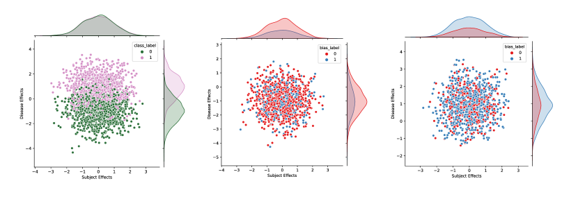
Figure 4: Kernel density estimate/scatter plots of subject and disease effect magnitude sampled from principal component analysis models. The distribution of subject effect magnitude within each target class, or the joint distribution of subject and disease effect magnitudes within each bias group can be identified by deep learning models and lead to performance disparities if there are differences between subgroups. Therefore, it is important to stratify such effects as shown in the figure to minimize this distribution-induced bias. The sampling distributions shown in the figure are identical for each bias scenario. Left: All samples, middle: non-disease class, right: disease class.

In this work, we extend this basic methodology to pre-define stratified distributions of subject and disease effect magnitude. Simply put, this ensures that the subject and disease effect magnitude distributions for each class and bias group are similar, which helps to prevent these distributions from introducing an additional, unwanted source of bias in deep learning models. This significant extension of SimBA is, therefore, crucial for the aim of this work. Further details are depicted in Supplementary Figure 4.

The datasets generated for this study used the SRI24 atlas (Rohlfing et al., 2010) with LPBA40 labels (Shattuck et al., 2008) as the brain template, with dimensions of 173×211×155 voxels and an isotropic resolution of 1 mm³. The morphological effects added to this template were derived from PCA models fit to stationary velocity fields of T1-weighted MRIs (Log-Euclidean framework (Arsigny et al., 2006)), which were obtained via non-linear diffeomorphic registration of 50 images from the IXI (brain development.org, ) database to the SRI24 atlas, as described in Stanley et al. (2023). Each full dataset generated for the experiments in this work is comprised of 2002 three-dimensional images of distinct simulated subjects, with two target classes (“disease”, N=1000, and “non-disease”, N=1002), and two bias groups (“bias”, containing an additional morphological effect, and “non-bias”, which does not contain such an effect). 70% of the images in the disease class were defined to belong to the bias group, while 30% of the images in the non-disease class were defined to belong to the bias group. With this unequal representation of the bias group in each class, it is expected that the deep learning model uses the presence of the bias effect as a shortcut for predicting the disease class, resulting in subgroup performance disparities.

Supplementary Table 2 provides the detailed dataset generation parameters. We defined the disease region, which contains the effects that are meant to act as the prediction target for the deep learning model, as the left insular cortex. Next, we generated datasets for three bias scenarios: 1) No Bias Effect, 2) “Near” Bias Effect (left putamen, adjacent to disease region), and 3) “Far” Bias Effect (right postcentral gyrus, opposite hemisphere as the disease region and on a different axial slice). These three bias scenarios are “paired” such that the images in each dataset contain the same subject effects and disease effects – in other words, each dataset acts as a counterfactual, where the same generated subjects have either no bias effect, or a bias effect in the near or far regions, respectively. Thus, evaluation of a model with identical weight initialization and deterministic training allows for direct comparison of the impact of each bias scenario on the deep learning pipeline. We applied this training schema for prediction of the target class from the imaging data using a convolutional neural network (CNN) (implementation details in A). CNNs automatically extract relevant features from images, making them a commonly used model architecture in medical image analysis where subtle details or patterns can be indicative of diseases or conditions.

2.2 Bias mitigation

To further showcase the utility of this framework, we quantitatively evaluated the efficacy of three conceptually different and representative bias mitigation strategies from the literature for each bias scenario. First, we applied reweighing, a pre-processing strategy proposed by Calders et al. (2009) that adds weights to each image during training to balance the contribution of bias groups in each target class. Second, we applied the in-processing adversarial bias “unlearning” strategy described in Dinsdale et al. (2021) which encourages the feature encoder to unlearn information required to predict the bias group label, while keeping disease classification performance high. Finally, we fine-tuned bias group models, following Puyol-Antón et al. (2021) by pretraining a model on the full dataset, and then training separate models for each bias group until convergence. Implementation details of the bias mitigation strategies are provided in A.

2.3 Evaluation

Model accuracy was used as a metric to determine efficacy in achieving the target prediction task of disease classification, where the disease class is a positive prediction, and the non-disease class is a negative prediction. Subgroup performance disparities, or the difference in true positive rate ($\Delta$TPR) and false positive rate ($\Delta$FPR) between the bias group and the non-bias group, were the primary outcome metrics for measuring bias (Equations 1, 2):

$$\Delta TPR=TPR_{bias\;group}-TPR_{non-bias\;group}$$ (1)

$$\Delta FPR=FPR_{bias\;group}-FPR_{non-bias\;group}$$ (2)

Standard deviations across five model seeds are reported as error values.

Exploiting the benefits of the counterfactual setup, we measured performance disparities relative to the baseline (No Bias) scenario (Equations 3, 4), since there are minimal but non-zero performance disparities due to differences in the underlying disease and subject effect distributions. Thus, any measured relative performance disparity between bias groups can be attributed purely to the presence of the morphological bias effects we wish to study.

$$Relative\;\Delta TPR=\Delta TPR-\Delta TPR_{No\;Bias}$$ (3)

$$Relative\;\Delta FPR=\Delta FPR-\Delta FPR_{No\;Bias}$$ (4)

2.4 Explainability

SmoothGrad (Smilkov et al., 2017) saliency maps were used to explore the extent to which the bias regions influenced the model in predicting the target class. Final saliency maps were generated from an average of 10 images from each bias group that were correctly classified as belonging to either the disease or non-disease class. Quantitative explainability is reported using weighted saliency scores (Stanley et al., 2022), which represents the relative intensity of salient voxels in a given brain region across the whole saliency map.

2.5 Statistics

We performed a two-way repeated measures ANOVA on $\Delta$TPR and $\Delta$FPR with bias scenario (No Bias, Near Bias, Far Bias) and bias mitigation method (naïve, reweighing, unlearning, group models) as the factors. Following significant effects, we performed Shapiro-Wilk tests to check for normality and two-tailed comparison tests (paired t-tests if normality test was passed, otherwise Wilcoxon matched-pairs signed rank test) with Bonferroni correction to compare between specific bias scenarios and mitigation methods (Supplementary Tables 4 and 5). The corrected significance level was $\alpha$=0.005. Analysis was performed in GraphPad Prism 10.0.2.

3 Results

3.1 Naïve model

All models trained using data from the three bias scenarios demonstrate high overall classification accuracy, with 84·81±0·62%, 87·68±0·20%, and 86·77±0·71% for the No Bias, Near Bias, and Far Bias datasets, respectively. The presence of the bias effect resulted in significant performance disparities compared to the No Bias scenario, with a relative $\Delta$TPR of 22·12±2·72% (p$<$0·0001) and $\Delta$FPR of 20·32±2·81% (p$<$0·0001) in the Near Bias scenario, and a relative $\Delta$TPR of 17·35±2·78% (p=0·0002) and relative $\Delta$FPR of 11·88±6·22% (p=0·0008) in the Far Bias scenario. These results indicate that the models likely used the bias effect as a shortcut for predicting the (positive) disease class, since the disease class contains a higher proportion of the bias group compared to the non-disease class. However, the models may have used this shortcut learning to a lesser extent when the bias region is farther from the disease region, as evidenced by the lower relative $\Delta$FPR and $\Delta$TPR in the Far Bias scenario compared to the Near Bias scenario.

Table 1: Performance of each bias mitigation strategy for each bias scenario. Errors are reported as standard deviation across five model seeds. Naïve=No bias mitigation, RW=reweighing, UL=unlearning, GM=group models, TPR=True positive rate, FPR=False positive rate.

Aggregate

Bias Group

Non-Bias Group

Naïve

RW

UL

GM

Naïve

RW

UL

GM

Naïve

RW

UL

GM

Accuracy (%)

No Bias

84.81 ± 0.62

85.01 ± 0.39

79.28 ± 2.76

-

85.24 ± 0.61

85.08 ± 0.64

79.84 ± 6.66

88.23 ± 0.34

84.38 ± 1.18

84.94 ± 0.44

78.73 ± 10.47

87.01 ± 0.78

Near Bias

87.68 ± 0.20

84.33 ± 0.39

86.65 ± 0.72

-

88.21 ± 0.39

84.68 ± 0.29

87.34 ± 1.05

88.06 ± 0.88

87.15 ± 0.75

83.98 ± 0.77

85.98 ± 1.07

87.41 ± 0.83

Far Bias

86.77 ± 0.71

84.89 ± 0.52

85.29 ± 0.99

-

87.10 ± 0.99

85.32 ± 0.36

85.48 ± 2.61

87.90 ± 0.40

86.45 ± 0.69

84.46 ± 0.75

85.10 ± 2.59

87.17 ± 0.71

TPR (%)

No Bias

85.73 ± 1.01

85.00 ± 1.67

80.24 ± 17.02

-

85.44 ± 0.91

84.78 ± 1.65

79.71 ± 20.57

93.44 ± 1.54

86.47 ± 1.61

85.59 ± 1.92

81.18 ± 17.96

70.59 ± 6.15

Near Bias

88.31 ± 0.74

84.44 ± 1.44

89.60 ± 4.34

-

93.89 ± 0.79

84.33 ± 1.44

92.67 ± 3.69

92.67 ± 2.56

73.53 ± 2.08

84.71 ± 1.68

81.4 ± 6.29

72.06 ± 1.80

Far Bias

85.08 ± 2.53

85.89 ± 0.29

85.24 ± 6.48

-

89.56 ± 3.10

85.44 ± 0.25

86.22 ± 5.91

92.67 ± 0.72

73.24 ± 1.92

87.06 ± 0.66

82.65 ± 8.54

72.94 ± 3.83

FPR (%)

No Bias

16.10 ± 1.28

14.98 ± 1.40

21.67 ± 20.70

-

15.28 ± 0.81

14.12 ± 3.05

20.29 ± 20.57

25.29 ± 2.87

16.39 ± 1.64

15.30 ± 0.86

22.19 ± 20.76

6.89 ± 1.26

Near Bias

12.95 ± 0.95

15.78 ± 1.53

16.25 ± 3.73

-

26.84 ± 2.21

14.41 ± 3.35

26.76 ± 6.10

24.12 ± 5.46

7.79 ± 1.63

16.28 ± 1.41

12.35 ± 3.01

6.89 ± 1.13

Far Bias

11.55 ± 1.67

16.10 ± 1.21

14.66 ± 6.13

-

19.41 ± 4.81

15.00 ± 1.61

16.47 ± 6.44

24.71 ± 1.23

8.63 ± 1.18

16.50 ± 1.18

13.99 ± 6.14

7.54 ± 1.25

Saliency maps highlighted both the disease and the corresponding bias region in each of the bias scenarios (Figure 1). Quantitatively, weighted saliency scores demonstrated a higher intensity saliency within the regions affected by the bias effect for both the Near and Far Bias scenarios relative to the No Bias baseline (Figure 3).

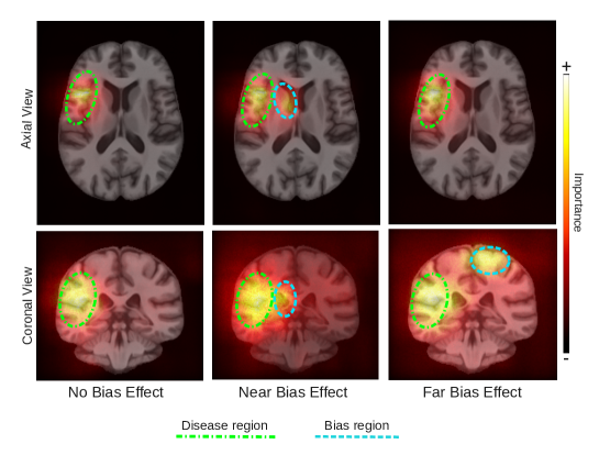
Figure 1: Average SmoothGrad saliency maps of correctly classified “subjects” for the bias group in the disease class, for each bias scenario in the naïve models.

3.2 Bias mitigated models

Each of the bias mitigated models demonstrated high overall classification accuracy, comparable to that of the naïve model (Table 1). It was also observed that all bias mitigation strategies reduce TPR and FPR disparities between the bias groups, albeit to different degrees (Figure 2).

The reweighing strategy almost perfectly mitigated any measured performance disparity between the bias groups, to respective values of relative $\Delta$TPR and relative $\Delta$FPR of 0·44±1·80% and –0·69±1·45% for the Near Bias scenario, and –0·80±0·64% and –0·32±2·13% for the Far Bias scenario.

The unlearning strategy also reduced the performance disparities between groups, although to a lesser degree. More precisely, the relative $\Delta$TPR was reduced to 12·22±3·04% for the Near Bias scenario and 4·60±4·20% for the Far Bias scenario. The relative $\Delta$FPR was reduced to 15·51±4·87% and 3·58±3·01% for the Near and Far Bias scenarios, respectively. Notably, unlearning reduced performance disparities to a greater degree for the Far Bias scenario compared to the Near Bias scenario. For all bias scenarios, the ability of the model to predict the bias label was reduced to chance level (Supplementary Table 6). Performing unlearning with the dataset for the No Bias scenario resulted in lower and more variable model performance across all metrics (Table 1).

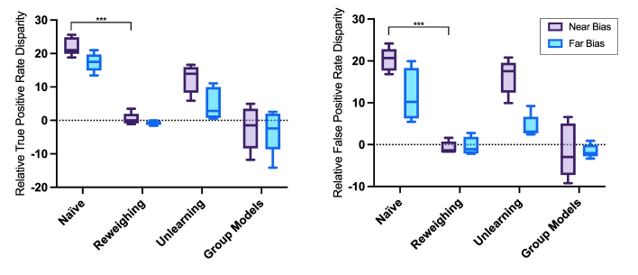
Figure 2: Relative true (left) and false (right) positive rate disparities between bias groups relative to the No Bias baseline for each bias mitigation strategy and bias scenario across five model seeds. Markers indicate significant differences between the naïve model performance ($\Delta$TPR, $\Delta$FPR) and each bias mitigation strategy (two-tailed paired t-test with Bonferroni correction, ***p$<$0·001).

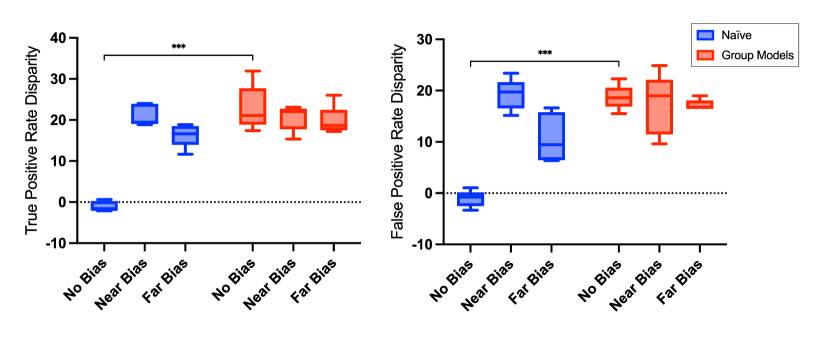
Figure 5: True (left) and false (right) positive rate disparities for the naïve models and group models. ***p$<$0.001.

Training separate models for each bias group also reduced the average $\Delta$TPR and $\Delta$FPR to near-zero, relative to the group models trained on the No Bias dataset. The relative $\Delta$TPR and $\Delta$FPR were –2·25±6·50% and –1·47±6·45% for the Near Bias scenario, and –3·13±6·62% and –1·54±1·59% for the Far Bias scenario. However, it was observed that the group model for the No Bias baseline demonstrated significant subgroup performance disparities compared to the No Bias naïve model ($\Delta$TPR=22·86±5·52%, p=0·0007 and $\Delta$FPR=18·70±2·42%, p=0·0001). Although the No Bias dataset did not have bias effects added, each bias group model was trained on a different number of images from each disease class (Supplementary Table 3), resulting in a typical class imbalance problem. Thus, while the addition of the near and far bias effects did not lead to any further performance disparities into the group models, we instead observed disparities implicitly introduced due to the different levels of bias group representation in each target class (Supplementary Figure 5).

Weighted saliency score results were in line with the efficacy of each bias mitigation strategy (Figure 3). For reweighing and group models, performance disparities were reduced to near-zero, and the corresponding saliency scores were similar to the No Bias baseline. The higher magnitude of performance disparities that remained after unlearning was reflected in the higher bias region saliency scores for this strategy.

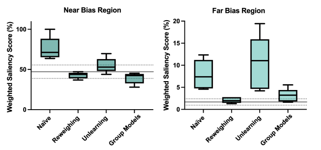
Figure 3: Weighted saliency scores calculated from average saliency maps over five model seeds for the bias group in the disease class for the brain regions most affected by “near” bias effect (left) and “far” bias effect (right). The horizontal line represents the weighted saliency score average ± standard deviation in the corresponding region for the No Bias naïve model.

4 Discussion

Overall, the results of this study highlight the utility and benefits of using the proposed analysis framework for performing a systematic and controlled evaluation of bias in medical imaging AI. We generated counterfactual neuroimaging datasets for three bias scenarios using an extended version of the SimBA tool and simulated in silico trials of each dataset with identical and deterministic deep learning pipelines. Since the exact bias effects that we aim to study in this setup are known, and it is also known how models perform on the counterfactual dataset without bias, the naïve models provide a strong baseline for objectively interpreting results of subsequent analyses. Thus, in the evaluation of each bias mitigation strategy, we can better understand the situations these mitigation strategies are effective in, or the reasons they may fail.

The results showed that reweighing completely mitigated performance disparities caused by the single source of bias we introduced. Thus, several real-world evaluations of reweighing (Larrazabal et al., 2020; Meissen et al., 2023; Puyol-Antón et al., 2021) may have been successful as a result of being applied to subgroups associated with the predominant sources of bias in the data. On the other hand, systematically introducing more complexity (e.g., additional sources of bias) to these synthetic datasets may help to improve our understanding why reweighing fails to alleviate performance disparities in various other real-world datasets (Ioannou et al., 2022; Meissen et al., 2023; Weng et al., 2023; Zhang et al., 2022). For the unlearning strategy, it was found that the model’s ability to predict the bias label was reduced to chance level, but this did not effectively mitigate subgroup performance disparities. This may be due to the bias features and the features necessary for predicting the target class being too similar to be fully disentangled. Understanding why this occurs likely requires deeper investigation into the model’s internal representations of disease and bias effects, which would be a straightforward task with these synthetic datasets since there are only two user-defined effects that the model can use for the prediction task. Furthermore, given the simulated counterfactual No Bias scenario, it can be seen that unlearning applied to this dataset even harms the model, resulting in lower performance on average and higher variability across model seeds. This finding is especially important considering that potential bias attributes in real-world datasets, such as scanner models or self-reported demographics, could be inaccurately labeled. Further work could be performed using this framework to analyze how mislabeling of bias attributes affects the result of this and other mitigation strategies. Moreover, the No Bias counterfactual datasets made it clear that performance disparities in the group models were not caused by the bias effects, but rather by the target class imbalance within each bias group. If this approach was used to de-bias a classification task on real data, the cause of these performance disparities may have been unclear since it could have been related to other subgroup attributes unaccounted for. Finally, we observed that the saliency scores align with performance of the model for each bias mitigation strategy. With knowledge of the exact regions that should be relevant for model decision-making, and of how a particular explainability method manifests in the absence of the bias effect, this framework facilitates a highly objective interpretation of explainable AI in medical imaging. Further work could use this setup for studying the extent to which different explainability methods highlight regions associated with predictive targets or bias effects, or developing new methods that are better at identifying salient regions of medical images.

Although the SimBA tool enables the generation of increasingly complex dataset bias scenarios, real-world medical imaging data can be even more complex than the synthetic data we analyze in this controlled setup. This is because real datasets inherently contain numerous confounding and interacting biases, many of which may be imperceptible to humans. For instance, it may be necessary to account for disease prevalence and population shift when evaluating performance disparities in real data, since the underlying distribution of other subgroup-associated factors may confound analysis. Glocker and colleagues (Glocker et al., 2023) account for this by performing test set resampling to balance the representation of subgroups for a more accurate representation of algorithmic bias. Conversely, using the SimBA data generation tool in our framework, these underlying distribution shifts can be mitigated, as we do here with stratified sampling, or systematically simulated and evaluated by generating datasets with shifts in the distributions of subject or disease effects. Thus, this analysis framework provides a powerful technique for investigating algorithmic encoding of bias and efficacy of bias mitigation strategies on a range of dataset bias scenarios, in which the biases could be represented by localized spatial deformations, sampled distribution of global morphology, or intensity-based simulated artifacts, to name a few. Therefore, models and methods can be studied and benchmarked on fully controlled setups prior to making conclusions on real-world data. The control and flexibility over the dataset composition provided by SimBA, and the ability to rigorously test in silico trials of the same simulated “subjects” with different bias manifestations as we present in this framework facilitates a comprehensive and objective exploration of biases in medical imaging AI, which was not previously possible.

This first feasibility study was limited by restricting the scope to simulation of spatially localized morphological bias effects in structural neuroimaging data and analysis of subsequent impacts on a single CNN model architecture. However, using this structured analysis framework as a baseline, we believe that there are numerous avenues that the research community hoping to gain a better understanding of bias in medical imaging AI can pursue. For instance, the potential relationship between the magnitude of performance disparities and proximity of disease and bias regions warrants further investigation into whether these results are consistent when using vision transformer-like architectures, where the model learns a more complex representation of global and local interactions than what is possible in a standard CNN. Furthermore, this framework could provide particular utility in the development of new bias mitigation strategies (especially unsupervised ones), since the user can ensure that all the sources of bias in the data are being addressed, which is not the case if such a strategy were to be evaluated on real data. Aside from studying other organs, arbitrary biases, and disease effects, clinical knowledge of well-defined pathologies (e.g., lesions) could be integrated to more faithfully model real diseases. Additionally, as users define the disease effects, predictive tasks are not limited to classification, but could also be extended to regression or segmentation scenarios.

In summary, this work introduced a structured framework for analyzing bias manifestation and mitigation in medical imaging AI. The results show that this framework has the potential to greatly improve understanding of bias in medical imaging deep learning pipelines, which alongside studies investigating the impacts of real-world biased data, will support the development of clinical AI tools that are more robust, responsible, and fair.

5 Data Sharing

Datasets, code, and train/validation/test splits are available for download from https://github.com/estanley16/SimBA.

6 Declaration of Interests

The authors have no competing interests to declare.

Appendix A Implementation Details

Model and Training. The convolutional neural network (CNN) we use for all experiments contains five convolutional blocks (filters=32, 64, 128, 256, 512) comprised of 3x3x3 convolution filters, batch normalization, sigmoid activation, and 2x2x2 max pooling, followed by average pooling, 20% dropout, a flatten layer, and a dense classification layer. A batch size of four and learning rate of 1e^-4 was used, and models were trained until convergence, by validation loss early stopping patience=15. For each bias scenario (No Bias, Near Bias, Far Bias), we trained the same model architecture using the same five weight initialization seeds with deterministic GPU state, in which each seed replicate uses the same dataset train, validation, and test splits of 50%/25%/25%. Each split was stratified by subject effects, disease effects, bias group label, and disease class label. Thus, evaluation of each bias scenario is a counterfactual of the same model and same dataset, where the difference is in the absence of the bias effect, or the bias effect in different locations. The models were implemented in Keras/Tensorflow v. 2.10 using a NVIDIA GeForce RTX 3090 GPU.

Reweighing. The weight W for samples in target class D and bias group B is given by:

$$W(B=b|D=d)=\dfrac{P_{exp}(b\land d)}{P_{exp}(b\land d)}$$

Where:

$$P_{exp}(b\land d)=\text{expected probability of an unbiased dataset.}$$

And:

$$P_{act}(b\land d)=\text{actual probability in dataset.}$$

Thus, the weights for each class and bias group are:

$$W(B=1|D=1)=\dfrac{d(\gamma+\alpha)}{\gamma}$$

$$W(B=1|D=0)=\dfrac{(1-d)(\gamma+\alpha)}{\alpha}$$

$$W(B=1=0|D=1)=\dfrac{d(2-\gamma-\alpha)}{1-\gamma}$$

$$W(B=0|D=0)=\dfrac{(1-d)(2-\gamma-\alpha)}{1-\alpha}$$

Where:

$$\alpha=\text{fraction of bias group in non-disease class.}$$

$$\gamma=\text{fraction of bias group in disease class.}$$

$$d=\text{fraction of disease class in full dataset.}$$

Bias Unlearning. The goal of the unlearning strategy is to modify the weights of the feature encoder (i.e., the entire CNN except for the dense classification layer) such that the model is no longer able to predict the bias group while retaining the ability to predict the disease. The same feature encoder backbone was used with two classification heads (i.e., the final dense layer), one for the disease classification and one for the bias group classification. First, the encoder and disease prediction head were trained until convergence. Then, the encoder was frozen and the disease prediction head was replaced with a bias prediction head, which was trained to convergence. Subsequently, the unlearning process takes place, in which the cross-entropy loss for predicting the disease is minimized, while a confusion loss for predicting the bias group is maximized. This iterative training takes place until the disease prediction accuracy has stopped improving and the bias prediction accuracy has stopped decreasing. In our experiments, only five epochs were necessary to unlearn the bias group. Bias prediction results are reported in Supplementary Table 6.

Group Models. First, the model was pre-trained for 5 epochs on the full dataset. Then, using the pre-trained model as a basis, separate models were trained on both the bias and non-bias groups. Accuracy, true positive rates, and false positive rates were computed for each group model individually, and then compared to get the reported subgroup performance disparities.

Appendix B Supplementary Tables

Table 2: SimBA effect sampling parameters.

Subject Disease Class Non-Disease Class Bias Group Non-Bias Group Number of Samples 2002 1000 1002 1003 999 Region Whole brain Left insular cortex Left insular cortex Near: Left putamen Far: Right postcentral gyrus - Sampling Distribution N(0,1)$\in$[-3.5,3.5] N(-1,1) N(1,1) N(2,1) - Number of Principal Components Sampled From 10 1 1 1 - Number of Stratification Bins 10 10 10 - -

Table 3: Composition of dataset splits.

Train Validation Test Disease Non-Disease Disease Non-Disease Disease Non-Disease Non-Bias 140 360 72 176 68 183 Bias 360 145 180 70 180 68

Table 4: True positive rate statistical tests. Bold font indicates groups in comparison test. Two-tailed paired t-test unless indicated by *, then Wilcoxon matched-pairs signed rank test. †significant after Bonferroni correction ($\alpha$=0.005).

Model Bias Scenario P-value Naïve No Bias – Near Bias <0.0001† Naïve No Bias – Far Bias 0.0002† Naïve Near Bias – Far Bias 0.1037 Naïve – Reweighing Near Bias 0.0001† Naïve – Unlearning Near Bias 0.0075 Naïve – Group Models Near Bias 0.8534 Naïve – Reweighing* Far Bias 0.0625 Naïve – Unlearning Far Bias 0.0104 Naïve – Group Models* Far Bias 0.0625 Naïve – Group Models No Bias 0.0007†

Table 5: False positive rate statistical tests. Bold font indicates groups in comparison test. Two-tailed paired t-test unless indicated by *, then Wilcoxon matched-pairs signed rank test. †significant after Bonferroni correction ($\alpha$=0.005).

Model Bias Scenario P-value Naïve No Bias – Near Bias <0.0001† Naïve No Bias – Far Bias 0.0008† Naïve Near Bias – Far Bias 0.0552 Naïve – Reweighing Near Bias 0.0002† Naïve – Unlearning Near Bias 0.0525 Naïve – Group Models Near Bias 0.6071 Naïve – Reweighing Far Bias 0.0058 Naïve – Unlearning* Far Bias 0.0625 Naïve – Group Models Far Bias 0.0289 Naïve – Group Models No Bias 0.0001†

Table 6: Results of bias group prediction after unlearning.

Bias Scenario Bias Prediction Accuracy (%) No Bias 49.94 ± 0.33 Near Bias 47.17 ± 4.23 Far Bias 46.73 ± 7.98

Table 7: Weighted saliency scores (%) for the Near Bias region across five model seeds.

Disease Class Non-Disease Class Bias Scenario Bias Mitigation Strategy Non-Bias Group Bias Group Non-Bias Group Bias Group No Bias Naïve 47.32 ± 7.23 47.18 ± 8.35 30.34 ± 7.55 30.55 ± 6.85 Reweighing 40.97 ± 4.37 39.88 ± 4.73 23.25 ± 5.97 23.48 ± 5.62 Unlearning 46.14 ± 7.66 44.98 ± 6.86 30.67 ± 6.84 29.52 ± 6.51 Group Models 46.91 ± 1.40 45.92 ± 6.64 30.76 ± 7.95 29.53 ± 8.58 Near Bias Naïve 77.09 ± 12.11 75.68 ± 14.42 45.78 ± 7.01 55.81 ± 16.84 Reweighing 41.76 ± 4.45 42.7 ± 3.89 19.22 ± 5.68 20.51 ± 5.52 Unlearning 59.64 ± 13.28 54.97 ± 9.37 36.02 ± 12.65 37.34 ± 13.98 Group Models 42.15 ± 4.03 39.28 ± 6.95 27.1 ± 4.92 21.59 ± 4.70

Table 8: Weighted saliency scores (%) for the Far Bias region across five model seeds.

Disease Class Non-Disease Class Bias Scenario Bias Mitigation Strategy Non-Bias Group Bias Group Non-Bias Group Bias Group No Bias Naïve 1.69 ± 0.76 1.67 ± 0.72 1.22 ± 0.42 1.14 ± 0.32 Reweighing 1.34 ± 0.70 1.31 ± 0.69 1.35 ± 0.67 1.34 ± 0.67 Unlearning 1.13 ± 0.52 1.12 ± 0.53 0.98 ± 0.25 0.95 ± 0.28 Group Models 1.91 ± 0.99 1.5 ± 0.55 1.59 ± 1.00 1.41 ± 0.63 Near Bias Naïve 7.77 ± 3.35 7.85 ± 3.32 7.47 ± 3.56 7.39 ± 3.55 Reweighing 2.23 ± 0.79 2.09 ± 0.66 1.48 ± 0.70 1.48 ± 0.70 Unlearning 10.47 ± 6.04 10.41 ± 6.16 8.66 ± 4.25 8.65 ± 4.46 Group Models 1.91 ± 0.60 3.12 ± 1.53 1.6 ± 0.49 2.64 ± 1.70

Appendix C Supplementary Figures

References

Adeli et al. (2021)
Adeli, E., Zhao, Q., Pfefferbaum, A., Sullivan, E.V., Fei-Fei, L., Niebles, J.C., Pohl, K.M., 2021.
Representation learning with statistical independence to mitigate bias, in: 2021 IEEE Winter Conference on Applications of Computer Vision (WACV), IEEE, Waikoloa, HI, USA. p. 2512–2522.
URL: https://ieeexplore.ieee.org/document/9423445/, doi:10.1109/WACV48630.2021.00256.
Arsigny et al. (2006)
Arsigny, V., Commowick, O., Pennec, X., Ayache, N., 2006.
A log-euclidean framework for statistics on diffeomorphisms, in: Larsen, R., Nielsen, M., Sporring, J. (Eds.), Medical Image Computing and Computer-Assisted Intervention – MICCAI 2006, Springer, Berlin, Heidelberg. p. 924–931.
doi:10.1007/11866565_113.
Banerjee et al. (2023)
Banerjee, I., Bhattacharjee, K., Burns, J.L., Trivedi, H., Purkayastha, S., Seyyed-Kalantari, L., Patel, B.N., Shiradkar, R., Gichoya, J., 2023.
“shortcuts” causing bias in radiology artificial intelligence: Causes, evaluation, and mitigation.
Journal of the American College of Radiology 20, 842–851.
doi:10.1016/j.jacr.2023.06.025.
Brown et al. (2023)
Brown, A., Tomasev, N., Freyberg, J., Liu, Y., Karthikesalingam, A., Schrouff, J., 2023.
Detecting shortcut learning for fair medical ai using shortcut testing.
Nature Communications 14, 4314.
doi:10.1038/s41467-023-39902-7.
Burns et al. (2023)
Burns, J.L., Zaiman, Z., Vanschaik, J., Luo, G., Peng, L., Price, B., Mathias, G., Mittal, V., Sagane, A., Tignanelli, C., Chakraborty, S., Gichoya, J.W., Purkayastha, S., 2023.
Ability of artificial intelligence to identify self-reported race in chest x-ray using pixel intensity counts.
Journal of Medical Imaging 10, 061106.
doi:10.1117/1.JMI.10.6.061106.
Calders et al. (2009)
Calders, T., Kamiran, F., Pechenizkiy, M., 2009.
Building classifiers with independency constraints, in: 2009 IEEE International Conference on Data Mining Workshops, IEEE, Miami, FL, USA. p. 13–18.
URL: http://ieeexplore.ieee.org/document/5360534/, doi:10.1109/ICDMW.2009.83.
Dinsdale et al. (2021)
Dinsdale, N.K., Jenkinson, M., Namburete, A.I.L., 2021.
Deep learning-based unlearning of dataset bias for mri harmonisation and confound removal.
NeuroImage 228, 117689.
doi:10.1016/j.neuroimage.2020.117689.
Gichoya et al. (2022)
Gichoya, J.W., Banerjee, I., Bhimireddy, A.R., Burns, J.L., Celi, L.A., Chen, L.C., Correa, R., Dullerud, N., Ghassemi, M., Huang, S.C., Kuo, P.C., Lungren, M.P., Palmer, L.J., Price, B.J., Purkayastha, S., Pyrros, A.T., Oakden-Rayner, L., Okechukwu, C., Seyyed-Kalantari, L., Trivedi, H., Wang, R., Zaiman, Z., Zhang, H., 2022.
Ai recognition of patient race in medical imaging: a modelling study.
The Lancet Digital Health 4, e406–e414.
doi:10.1016/S2589-7500(22)00063-2.
Glocker et al. (2023)
Glocker, B., Jones, C., Bernhardt, M., Winzeck, S., 2023.
Algorithmic encoding of protected characteristics in chest x-ray disease detection models.
eBioMedicine 89, 104467.
doi:10.1016/j.ebiom.2023.104467.
Ioannou et al. (2022)
Ioannou, S., Chockler, H., Hammers, A., King, A.P., 2022.
A study of demographic bias in cnn-based brain mr segmentation, in: Abdulkadir, A., Bathula, D.R., Dvornek, N.C., Habes, M., Kia, S.M., Kumar, V., Wolfers, T. (Eds.), Machine Learning in Clinical Neuroimaging, Springer Nature Switzerland, Cham. p. 13–22.
doi:10.1007/978-3-031-17899-3_2.
Jones et al. (2023)
Jones, C., Roschewitz, M., Glocker, B., 2023.
The role of subgroup separability in group-fair medical image classification, in: Greenspan, H., Madabhushi, A., Mousavi, P., Salcudean, S., Duncan, J., Syeda-Mahmood, T., Taylor, R. (Eds.), Medical Image Computing and Computer Assisted Intervention – MICCAI 2023, Springer Nature Switzerland, Cham. p. 179–188.
doi:10.1007/978-3-031-43898-1_18.
Larrazabal et al. (2020)
Larrazabal, A.J., Nieto, N., Peterson, V., Milone, D.H., Ferrante, E., 2020.
Gender imbalance in medical imaging datasets produces biased classifiers for computer-aided diagnosis.
Proceedings of the National Academy of Sciences 117, 12592–12594.
doi:10.1073/pnas.1919012117.
Marcinkevics et al. (2022)
Marcinkevics, R., Ozkan, E., Vogt, J.E., 2022.
Debiasing deep chest x-ray classifiers using intra- and post-processing methods, in: Proceedings of the 7th Machine Learning for Healthcare Conference, PMLR. p. 504–536.
URL: https://proceedings.mlr.press/v182/marcinkevics22a.html.
Meissen et al. (2023)
Meissen, F., Breuer, S., Knolle, M., Buyx, A., Müller, R., Kaissis, G., Wiestler, B., Rückert, D., 2023.
(predictable) performance bias in unsupervised anomaly detection URL: http://arxiv.org/abs/2309.14198. arXiv:2309.14198 [cs, eess].
Piçarra and Glocker (2023)
Piçarra, C., Glocker, B., 2023.
Analysing race and sex bias in brain age prediction, in: Wesarg, S., Puyol Antón, E., Baxter, J.S.H., Erdt, M., Drechsler, K., Oyarzun Laura, C., Freiman, M., Chen, Y., Rekik, I., Eagleson, R., Feragen, A., King, A.P., Cheplygina, V., Ganz-Benjaminsen, M., Ferrante, E., Glocker, B., Moyer, D., Petersen, E. (Eds.), Clinical Image-Based Procedures, Fairness of AI in Medical Imaging, and Ethical and Philosophical Issues in Medical Imaging, Springer Nature Switzerland, Cham. p. 194–204.
doi:10.1007/978-3-031-45249-9_19.
Puyol-Antón et al. (2021)
Puyol-Antón, E., Ruijsink, B., Piechnik, S.K., Neubauer, S., Petersen, S.E., Razavi, R., King, A.P., 2021.
Fairness in cardiac mr image analysis: An investigation of bias due to data imbalance in deep learning based segmentation, in: de Bruijne, M., Cattin, P.C., Cotin, S., Padoy, N., Speidel, S., Zheng, Y., Essert, C. (Eds.), Medical Image Computing and Computer Assisted Intervention – MICCAI 2021, Springer International Publishing, Cham. p. 413–423.
doi:10.1007/978-3-030-87199-4_39.
Rohlfing et al. (2010)
Rohlfing, T., Zahr, N.M., Sullivan, E.V., Pfefferbaum, A., 2010.
The sri24 multichannel atlas of normal adult human brain structure.
Human Brain Mapping 31, 798–819.
doi:10.1002/hbm.20906.
Seyyed-Kalantari et al. (2021)
Seyyed-Kalantari, L., Zhang, H., McDermott, M.B.A., Chen, I.Y., Ghassemi, M., 2021.
Underdiagnosis bias of artificial intelligence algorithms applied to chest radiographs in under-served patient populations.
Nature Medicine 27, 2176–2182.
doi:10.1038/s41591-021-01595-0.
Shattuck et al. (2008)
Shattuck, D.W., Mirza, M., Adisetiyo, V., Hojatkashani, C., Salamon, G., Narr, K.L., Poldrack, R.A., Bilder, R.M., Toga, A.W., 2008.
Construction of a 3d probabilistic atlas of human cortical structures.
NeuroImage 39, 1064–1080.
doi:10.1016/j.neuroimage.2007.09.031.
Smilkov et al. (2017)
Smilkov, D., Thorat, N., Kim, B., Viégas, F., Wattenberg, M., 2017.
Smoothgrad: removing noise by adding noise.
arXiv:1706.03825 [cs, stat] URL: http://arxiv.org/abs/1706.03825. arXiv: 1706.03825.
Souza et al. (2023)
Souza, R., Wilms, M., Camacho, M., Pike, G.B., Camicioli, R., Monchi, O., Forkert, N.D., 2023.
Image-encoded biological and non-biological variables may be used as shortcuts in deep learning models trained on multisite neuroimaging data.
Journal of the American Medical Informatics Association , ocad171doi:10.1093/jamia/ocad171.
Stanley et al. (2023)
Stanley, E.A.M., Wilms, M., Forkert, N.D., 2023.
A flexible framework for simulating and evaluating biases in deep learning-based medical image analysis, in: Greenspan, H., Madabhushi, A., Mousavi, P., Salcudean, S., Duncan, J., Syeda-Mahmood, T., Taylor, R. (Eds.), Medical Image Computing and Computer Assisted Intervention – MICCAI 2023, Springer Nature Switzerland, Cham. p. 489–499.
doi:10.1007/978-3-031-43895-0_46.
Stanley et al. (2022)
Stanley, E.A.M., Wilms, M., Mouches, P., Forkert, N.D., 2022.
Fairness-related performance and explainability effects in deep learning models for brain image analysis.
Journal of Medical Imaging 9, 061102.
doi:10.1117/1.JMI.9.6.061102.
Weng et al. (2023)
Weng, N., Bigdeli, S., Petersen, E., Feragen, A., 2023.
Are sex-based physiological differences the cause of gender bias for chest x-ray diagnosis?, in: Wesarg, S., Puyol Antón, E., Baxter, J.S.H., Erdt, M., Drechsler, K., Oyarzun Laura, C., Freiman, M., Chen, Y., Rekik, I., Eagleson, R., Feragen, A., King, A.P., Cheplygina, V., Ganz-Benjaminsen, M., Ferrante, E., Glocker, B., Moyer, D., Petersen, E. (Eds.), Clinical Image-Based Procedures, Fairness of AI in Medical Imaging, and Ethical and Philosophical Issues in Medical Imaging, Springer Nature Switzerland, Cham. p. 142–152.
doi:10.1007/978-3-031-45249-9_14.
Wu et al. (2022)
Wu, Y., Zeng, D., Xu, X., Shi, Y., Hu, J., 2022.
Fairprune: Achieving fairness through pruning for dermatological disease diagnosis, in: Wang, L., Dou, Q., Fletcher, P.T., Speidel, S., Li, S. (Eds.), Medical Image Computing and Computer Assisted Intervention – MICCAI 2022, Springer Nature Switzerland, Cham. p. 743–753.
doi:10.1007/978-3-031-16431-6_70.
Yearley et al. (2023)
Yearley, A.G., Goedmakers, C.M.W., Panahi, A., Doucette, J., Rana, A., Ranganathan, K., Smith, T.R., 2023.
Fda-approved machine learning algorithms in neuroradiology: A systematic review of the current evidence for approval.
Artificial Intelligence in Medicine 143, 102607.
doi:10.1016/j.artmed.2023.102607.
Zhang et al. (2022)
Zhang, H., Dullerud, N., Roth, K., Oakden-Rayner, L., Pfohl, S., Ghassemi, M., 2022.
Improving the fairness of chest x-ray classifiers, in: Proceedings of the Conference on Health, Inference, and Learning, PMLR. p. 204–233.
URL: https://proceedings.mlr.press/v174/zhang22a.html.