Feature Attribution Explanations for Spiking Neural Networks

Abstract

Third-generation artificial neural networks, Spiking Neural Networks (SNNs), can be efficiently implemented on hardware. Their implementation on neuromorphic chips opens a broad range of applications, such as machine learning-based autonomous control and intelligent biomedical devices. In critical applications, however, insight into the reasoning of SNNs is important, thus SNNs need to be equipped with the ability to explain how decisions are reached. We present Temporal Spike Attribution (TSA), a local explanation method for SNNs. To compute the explanation, we aggregate all information available in model-internal variables: spike times and model weights. We evaluate TSA on artificial and real-world time series data and measure explanation quality w.r.t. multiple quantitative criteria. We find that TSA correctly identifies a small subset of input features relevant to the decision (i.e., is output-complete and compact) and generates similar explanations for similar inputs (i.e., is continuous). Further, our experiments show that incorporating the notion of absent spikes improves explanation quality. Our work can serve as a starting point for explainable SNNs, with future implementations on hardware yielding not only predictions but also explanations in a broad range of application scenarios. Source code is available at https://github.com/ElisaNguyen/tsa-explanations.

I Introduction

Spiking neural networks (SNNs), also known as third-generation artificial neural networks [Maass.1997], consist of spiking neurons. Spiking neurons emit spikes at certain points in time to transmit information, similar to action potentials in biological neurons and are thus close to biological reality [Gerstner.2014]. SNNs are at least as powerful as deep artificial neural networks with continuous activation functions (ANNs) [Maass.1997]. Their applicability to supervised, unsupervised and reinforcement learning are active research areas [Ponulak2011-tt]. However, the predictive performance of SNNs is not yet on par with ANNs due to the non-differentiability of spikes, making SNN optimization an active research field [Wang.2020]. Nonetheless, SNNs are interesting as they yield the potential to be implemented in neuromorphic hardware, which is energy- and memory-efficient [Murray.1998]. Moreover, studies show improved adversarial robustness of SNNs [sharmin.2019]. Their inherent temporal nature also lends itself naturally to processing temporal data making them suitable for critical domains relying on sensor data such as autonomous control [Bing.2018] and applications using biomedical signals [azghadi.2020].

Critical domains, for example medical applications, pose specific requirements to machine learning models. In addition to high predictive performance, models should make predictions based on the right reasons and be transparent about their decision-making process [He.2019]. Exposing important information of machine learning models is the focus of research on EXplainable Artificial Intelligence (XAI) [Adadi.2018, Guidotti.2019]. Model explanations address the requirement for algorithm transparency and provide methods to inspect model behavior [Molnar.19102020]. While various explanation methods exist for second-generation artificial neural networks (ANNs) [Guidotti.2019, Adadi.2018], to the best of our knowledge, the current body of work in explaining SNNs only comprises two major works, namely [Jeyasothy.28022019, kim2021]. XAI for SNNS is thus yet a sparsely studied research area. If left unaddressed, this research gap could lead to situations where SNNs are methodologically mature for real-world deployment but remain unused because they lack transparency.

We contribute to the field of XAI for SNNs by presenting Temporal Spike Attributions (TSA), an SNN-specific explanation method. The resulting explanations are local, i.e., explain a particular prediction and answer the question: ‘Why did the model make this decision?’ [Adadi.2018]. We build on the explanation method of [kim2021] which uses the model’s spike trains. We additionally include the SNN’s weights to consider all model-internal variables and regard the absence of spikes to be informative as it also impacts the resulting spike patterns. TSA results in more complete and correct explanations due to the utilization of comprehensive model-internal information. We demonstrate TSA on time series data. In contrast to anecdotal evidence which is mainly used to evaluate XAI methods [nauta2022anecdotal], we systematically evaluate TSA quantitatively w.r.t. multiple aspects relevant to explanation quality: The correctness of the explanations (correctness), the explanation’s ability to capture the complete model behavior (output-completeness), sensitivity to input changes (continuity), and explanation size (compactness). In summary, our contributions are as follows:

1. We present Temporal Spike Attribution (TSA), a local feature attribution method for SNNs inferred from all model internal variables.

2. We apply Kim & Panda’s [kim2021] explanation method, which uses only spike train information, on time series data as a baseline to show the impact of incorporating all model internal information in TSA.

3. We thoroughly validate TSA’s explanation performance using a multi-faceted quantitative evaluation of feature attribution explanations for SNNs, evaluating correctness, completeness, continuity and compactness.

Because SNNs are more popular in neuroscience than machine learning, we briefly introduce SNNs in Section II. Section III reviews related works on SNN explainability. We reflect on the effect of SNN-internal variables on a prediction and present our explanation method, TSA, capturing these effects in Section IV. The multi-faceted evaluation in Sections LABEL:sec:experiments and LABEL:sec:results shows the improved explanation performance of TSA. We discuss results in Section LABEL:sec:discussion and conclude in Section LABEL:sec:conclusion.

II Spiking Neural Networks

This section introduces SNNs and their components. SNNs are characterized by their computational units, spiking neurons [Gerstner.2014]. Analogous to traditional ANNs, SNNs are networks of spiking neurons with weighted connections. SNNs process information in the form of spike trains, i.e., spikes over time. Neuron models differ in the spike generation mechanisms. Our proposed method is independent of the chosen spike generation mechanism. Without loss of generality, we employ the commonly used leaky integrate-and-fire (LIF) neuron model (cf. Figure 1). The membrane potential $u$ of a LIF neuron can be modeled with a linear differential equation:

$$\tau_{m}\frac{du}{dt}=-[u(t)-u_{\textrm{rest}}]+I(t),$$ (1)

where $I(t)$ describes the amount by which $u$ changes to external input. $\tau_{m}$ is the time constant of the neuron, which dictates the decay of $u$ in time. A LIF neuron fires when $u(t)$ crosses a threshold $\theta$ from below. Upon firing a spike, the membrane potentials of the postsynaptic neurons are changed by the weight value, as the spikes are propagated forward in the network. The sign of the weight defines the synapses’ nature (i.e., inhibitory or excitatory) and the weight value defines the strength of the postsynaptic potential. After firing, $u$ is reset to a low reset potential $u_{r}$, and then slowly increases back to its resting value $u_{\textrm{rest}}$.

SNNs internally process spike trains and thus require input data in the form of spikes. The translation of non-spiking to spiking data is called neural coding. Different neural codes exist with temporal and rate coding being the most common. Temporal coding is biologically more plausible than rate coding because it emphasizes exact spike times as information carriers [Gerstner.2014].

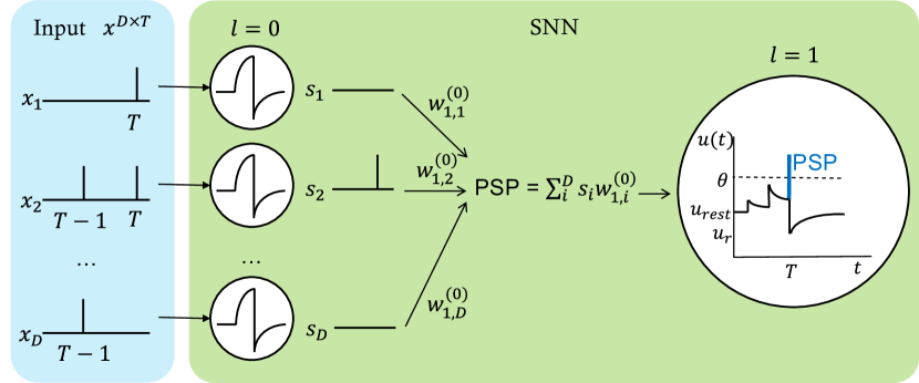
Figure 1: Schematic overview of an SNN with LIF neurons. Input spikes $x_{i}$ are fed to the SNN. Internally, it transmits information as spike patterns $s_{i}$, which are propagated forward with weights $w_{j,i}^{(l)}$ to determine the postsynaptic potential (PSP). The state of the postsynaptic neuron $u_{j}$ is changed by the PSP.

III Related Work

Our work is positioned in the field of EXplainable Artificial Intelligence (XAI) for SNNs. XAI researches methods to address the black-box nature of machine learning models and explain their reasoning to laypersons and experts  [Molnar.19102020]. Machine learning models can either be explained globally by providing an overview of the whole model, or locally by explaining single predictions. Global explanations aim at providing a global understanding of how input relates to an outcome distribution addressing the model explanation and model inspection problem [Adadi.2018, Guidotti.2019]. Examples of global explanation methods are [pmlr-v80-kim18d] and [Nauta2021NeuralPT]. The complexity of global explanations increases with the number of input features and model parameters and is therefore a challenging problem in XAI. Local explanations target individual model predictions and address the outcome explanation problem [Adadi.2018, Guidotti.2019], i.e. they explain the relation between a specific model input and output. Two prominent examples of local explanations are LIME [ribeiro_2016_lime] and SHAP [lundberg_lee_2017_shap]. We aim to explain predictions of SNNs and develop a local explanation method.

III-A Explaining Spiking Neural Networks

TABLE I: Comparison of our method (TSA) to related work FSF [Jeyasothy.28022019] and SAM [kim2021] in terms of XAI taxonomy [Adadi.2018] and evaluation [nauta2022anecdotal]. Completeness refers to output-completeness.

	FSF [Jeyasothy.28022019]	SAM [kim2021]	TSA (Ours)
XAI Method	Post-hoc	Post-hoc	Post-hoc
Scope	Global	Local	Local
Data type	Tabular	Images	Time-series
Model	MC-SEFRON	Convolutional SNNs	Specific to SNNs
Evaluation
Correctness	$\checkmark$	$\times$	$\checkmark$
Completeness	$\times$	$\times$	$\checkmark$
Continuity	$\times$	$\times$	$\checkmark$
Compactness	$\times$	$\times$	$\checkmark$
Coherence	$\times$	$\checkmark$	$\times$

Few works have studied explaining SNNs, which we introduce in the following. Jeyasothy et al. [Jeyasothy.28022019] present feature strength functions (FSFs) to explain a specific SNN model architecture MC-SEFRON with a population encoding layer, no hidden layers, and time-dependent weights. FSFs invert the population coding scheme to link the explanation back to input features and extract interpretable knowledge. FSFs are functions of the input, i.e. in a human-understandable domain rather than the temporal domain of spike trains. The FSFs are a global and model-specific explanation method, which addresses the model inspection problem [Guidotti.2019]. In contrast, we target local explanations to explain model decisions that are applicable to a wider range of SNN models.

Kim & Panda [kim2021] present Spike Activation Map (SAM), a local explanation method for SNNs. SAM generates visual heatmaps based on a calculation of input feature importance (in the image classification case, these are pixels) and was studied on deep convolutional SNNs with LIF neurons on image data. SAM is inspired by the biological observation that short inter-spike intervals are deemed to carry information because they likely cause a postsynaptic spike. The authors define contribution scores of single spikes and aggregate them to represent the spike train contribution in the neuronal contribution score (NCS). The final activation map is computed at time $t$ by a forward pass in the network by multiplying NCS’s at $t$ and summarizing NCS’s across the channel axis of convolutional layers. In contrast to the model-specific FSFs [Jeyasothy.28022019], NCSs are model-agnostic because they are solely based on spike information which is part of all SNNs.

Our explanation method TSA is model-agnostic but not model-independent because TSA also takes the model’s weights into account, which represent what the SNN has learned. Furthermore, we aim to cater to the intrinsic temporal design of SNNs and therefore designed TSA for explaining predictions of a time series classification task. We look at time series data as opposed to image data to better fit the temporal nature of SNNs. Thus, we contribute to local explanations for SNNs and compare TSA to SAM.

Table I presents a concise comparison of the related work and our explanation method. We do not compare to model-agnostic methods for ANNs (e.g., LIME [ribeiro_2016_lime]) because their application to SNNs is not trivial. Moreover, ANN-based explanations do not rely on SNN model internals and hence might not capture the true model behavior [Poyiadzi2021OnTO]. Our aim is an SNN-specific explanation method.

III-B Evaluating SNN Explanations

In contrast to evaluating the predictive performance of models with quasi-standard evaluation metrics (e.g., F-score, AUC), evaluating explanations is an ongoing research topic. Since the recipients of explanations are humans and are usually context-dependent, there is no standard evaluation protocol [Molnar.19102020]. In addition, a good explanation fulfills several different properties, e.g. the correctness or faithfulness in explaining the model behavior and human-comprehensibility among others [nauta2022anecdotal, ijcai/BhattWM20, ijcai/0002C20]. Moreover, evaluating explanations is challenging because the ground truth (what the model actually learned) is rarely known. To overcome this issue, one could apply the “Controlled Synthetic Data Check” [nauta2022anecdotal] where a model is applied to (structured) synthetic datasets such that the true data distribution is known, e.g. [liu_synthetic_2021]. We apply this method by constructing a synthetic data set for a classification problem on two input sensors (cf. Section LABEL:ssec:experiments:datasets).

The evaluations of FSFs and SAM were each focused on one aspect of explanation quality: Jeyasothy et al. [Jeyasothy.28022019] evaluated “reliability” by using FSFs instead of model weights in the same prediction task, testing how correctly the FSFs capture the global model behavior. Kim & Panda [kim2021] tested the “accuracy” of SAM by comparison with an existing heatmap explanation on ANNs, i.e. how coherent and aligned SAM explanations are to other explanations. In our work, we perform a multi-faceted evaluation based on the Co-12 framework for evaluating XAI [nauta2022anecdotal] on a synthetic and a real-world data set. More specifically, we evaluate correctness, output-completeness, continuity, and compactness as defined by Nauta et al. [nauta2022anecdotal]. We chose this subset of Co-12 properties as we focus on studying the content of TSA explanations first before considering presentation- and user-related properties.

IV Temporal Spike Attribution (TSA)

SNNs learn internal weights during training and process data as spike trains (cf. Section II. Whereas the Spike Activation Map (SAM) [kim2021] considers only spike trains to generate explanations, TSA captures all information available in the model for a prediction $\hat{y}$ at time $T$ of one $D$-dimensional input $x^{D\times T}$. These information are (i) spike times $S^{(l)}$, (ii) learned weights $W$, and (iii) membrane potentials at the output layer $U^{(L)}$. Each component has an influence on the output $\hat{y}$ and therefore should be included in the explanation. We explain the single components in Sections IV-A to IV-C and describe their integration to a feature attribution explanation in Section IV-D.

IV-A Influence of Hidden Neuron Spike Times

In temporal coding, the information about the data is assumed to be in the exact spike times of a neuron [Gerstner.2014]. The spike times indicate the attribution of neurons $I$ to their downstream neurons $J$ and represent the model’s activation in a prediction. Hence, the spike times influence the prediction. The relationship between the spike times of $I$ and their attribution to $J$ is captured in [kim2021]’s neuronal contribution score (NCS). The NCS is characterized by $\gamma$, which specifies the steepness of the exponential decay over time. We define the decay at the same rate as the decay of the LIF neuron’s membrane potential $u$ to reflect the dynamics of the model.

While we build on the NCS, our spike time component $N_{i}(t)$ additionally considers the absence of spikes as information carriers. In a fully connected SNN, each neuron of layer $l$ is connected with each neuron of layer $l+1$. The weighted sum of the neuron’s spiking behavior in $l$ determines the amount by which the membrane potentials of neurons in $l+1$ are changed. Absent spikes do not contribute to this sum. Hence, if a neuron $i$ does not spike at time $t$, it does not contribute actively to a change in $J$, allowing a natural decay. Absent spikes can thus be understood in two ways: (i) an absent spike does not affect $u_{j}$ (cf. Eq. 2) or (ii) an absent spike affects $u_{j}$ by not changing $u_{j}$ and letting it decay naturally (cf. Eq. 3). In the second case, the attribution of absent spikes to the postsynaptic neuron is negative. However, absent spike attribution should not weigh as much as spikes because their effect is highly dependent on other incoming synapses. We weigh the contribution of absent spikes by $\frac{1}{B}$ as an approximation of their attribution factor, with $B$ being the size of the preceding layer. This approximation is simple and reflects the relative magnitude of a non-spiking neuron’s attribution. Formally, we calculate the spike time component $N_{i}(t)$ as follows:

$$\small N^{S}_{i}(t) =\sum_{t^{\prime}=0}^{t}\begin{cases}\exp(-\gamma|t-t^{\prime}|)&\text{if }x_{i,t^{\prime}}=1\\ 0&\text{Otherwise}\end{cases}$$ (2)

only considering the presence of spikes, and

$$\small N^{NS}_{i}(t) =\sum_{t^{\prime}=0}^{t}\begin{cases}\exp(-\gamma|t-t^{\prime}|)&\text{if }x_{i,t^{\prime}}=1\\ -\frac{1}{B}\exp(-\gamma|t-t^{\prime}|)&\text{Otherwise}\end{cases}$$ (3)

when including the information about absent spikes.

In our experiments, we compare both variants as TSA^S (spikes only according to Eq. 2), and TSA^NS (non spikes included, according to Eq. 3).

IV-B Influence of Model Weights

The weights $W$ represent the strengths of connections of an SNN and have so far not been considered in feature attribution explanations for SNNs. We specifically include weights to capture the contribution of connections to the predictions of an SNN. Weights determine the impact of spikes to downstream neurons $J$ directly, where the weight value indicates the weight’s attribution to a neuron $j\in J$, and the sign specifies whether the synapse is excitatory or inhibitory and leads to an in- or decrease of $u_{j}$. Since weights are a property of the model, i.e. independent of the input, the weight contribution obtains its meaning in combination with other components.

IV-C Influence of Output Layer

The output layer is the last computational layer, i.e., the basis for prediction. The output layer consists of spiking neurons, thus the prediction is dictated either by spike patterns $S^{(L)}$ or membrane potentials $U^{(L)}$. In the first case, the influence of the output layer can be captured by the NCS. The SNN models in our work follow [Neftci.2019]’s architecture and make predictions based on the latter, i.e. the largest $u_{i}^{(L)}$ determines the predicted class. We capture the effect of the output layer on a model prediction by considering the classification softmax probability $P(t)$ in the computation of an explanation.

$$\vec{P}(t)=\text{softmax}(U^{(L)})$$ (4)

IV-D Computation of TSA

TSA combines neuron spike times, model weights, and output layer information in a forward pass into a final score as shown in Algorithm 1. A neuron $i$ generates spike train $s_{i}$ to the downstream computational layers. The neuron is connected to the next layer $l+1$ via the weight matrix $W^{(l)}$. Spike time information is captured by $\vec{N}^{(l)}(t)$, model weights are contained in $W$, and output layer information, i.e. membrane potentials are encoded in $\vec{P}(t)$. The spike times and the weights are combined by multiplying the diagonal matrix of $\vec{N}^{(l)}(t_{c})$ with $W^{(l)}$ per layer (line 7 in Algorithm 1). The resulting matrix can be computed for the input layer and all hidden layers. The result is a set of matrices consisting of scores that represent how the presynaptic neurons contribute to the postsynaptic neurons under direct consideration of the weights. The values are aggregated in a forward pass through the model. This represents how the input influences the model’s neurons and is captured by the input contribution $C_{I}(t)$ (Line 8). The final feature attribution $A(x,t)\in\mathbb{R}^{O\times D\times t}$ is computed by multiplying $C_{I}(t)$ with the softmax probabilities (Line 10). The absence of spikes can be understood as either not affecting (Eq. 2) or affecting downstream neurons (Eq. 3). We compare both variants as TSA^S (spikes only), and TSA^NS (non spikes included). Thus, the computation in line 6 of Algorithm 1 differs respectively.

Algorithm 1 Temporal Spike Attribution

Let $x\in\mathbb{R}^{D\times T}$ be an input to SNN $f$ with $L$ layers, $S^{(l)}$ a layer’s spike trains, $U^{(L)}$ the output layer’s membrane potentials, $W^{(l)}$ the weight matrix connecting layers $l$ and $l+1$, and $t$ the explanation time.

1:  $S^{(1)},...,S^{(L-1)},U^{(L)}\leftarrow f(x)$

2:  $\vec{P}(t)\leftarrow\text{softmax}(U^{(L)})$

3:  for $t^{\prime}=0,1,2,...,t$ do

4:     Initialize $C_{I}(t^{\prime})=I\in\mathbb{R}^{DxD}$

5:     for $l=1,2,...,L-1$ do

6:        Compute $\vec{N}^{(l)}(t^{\prime})$

7:        $N_{W}^{(l)}(t^{\prime})\leftarrow\text{diag}[\vec{N}^{(l)}(t^{\prime})]\cdot W^{(l)}$

8:        $C_{I}(t^{\prime})\leftarrow C_{I}(t^{\prime})\cdot N_{W}^{(l)}(t^{\prime})$

9:     end for

10:     $A(x,t^{\prime})\leftarrow C_{I}(t^{\prime})\cdot\text{diag}(\vec{P}(t^{\prime}))$

11:     Concatenate $A(x,t^{\prime})$ to attribution map $A(x,t)$.

12:  end for