Dispersion and absorption effects in the linearized Born-Infeld electrodynamics under an external magnetic field

Abstract

The effects of the Ohmic and magnetic density currents are investigated in the linearized Born-Infeld electrodynamics. The linearization is introduced through an external magnetic field, in which the vector potential of the Born-Infeld electrodynamics is expanded around of a magnetic background field, that we consider uniform and constant in this paper. From the Born-Infeld linearized equations, we obtain the solutions for the refractive index associated with the electromagnetic wave superposition, when the current density is ruled by the Ohm law, and in the second case, when the current density is set by a isotropic magnetic conductivity. These solutions are functions of the magnetic background $({\bf B})$, of the wave propagation direction $({\bf k})$, and also it depends on the material conductivity, and on the wave frequency. As consequence, the dispersion and the absorption of waves change when ${\bf B}$ is parallel to ${\bf k}$ in relation to the case of ${\bf B}$ perpendicular to ${\bf k}$ in the material medium. These characteristics of the refraction index related to directions of ${\bf B}$ and ${\bf k}$ open a discussion of the birefringence in the material medium.

I Introduction

The Born-Infeld (BI) electrodynamics (ED) is one of most famous non-linear extensions of the Maxwell ED in the literature [1]. Originally, it was proposed to explain the classical electron self-energy, since that, in Maxwell ED, the electric field for a rest like-point charge is not defined at the origin. After some years, the Euler-Heisenberg ED was discovered through the radiative corrections of the quantum electrodynamics, when it is submitted to the external electromagnetic field [2]. Nowadays, several examples of non-linear EDs have applications or solutions in many research areas, as anomalous couplings in physics beyond the Standard Model, black holes, string theory, Dirac materials and others, see the refs. [4, 3, 5, 6, 7, 8, 9]. The investigation of phenomena under action of an external field also is a subject of interest in non-linear EDs [10, 11]. The introduction of the external electromagnetic field in non-linear EDs is an approach that allows the investigation of propagation effects, as the dispersion relations, group velocities, the refractive index, and also the characteristics of the material medium under an external (uniform and constant) magnetic field [12, 13, 14]. The study of electromagnetic waves in materials, as conductors, is one of known applications of the Ohm law at room temperature [15]. It allows to obtain the dispersion and absorption of waves in the material medium. Other current density discussed in the literature of material physics is known as the magnetic current. The current density vector is proportional to the magnetic field, in which the proportionality constant is called magnetic conductivity [16, 17, 18]. This current density has origin from the systems with asymmetry of left- and right-handed chiral fermions, that is known as the Chiral Magnetic Effect. In Weyl semimetals, the CME is related to massless fermions acquire velocity along the magnetic field [19, 20].

Meeting all these motivations, we investigate the dispersion and absorption of the wave propagation in the linearized BI ED by an external magnetic field, when the material medium is governed by the current density of the Ohm law, and posteriorly, when the current density is the magnetic one. The refractive index of the material medium depends on the conductivity, on the wave frequency, and also on the magnetic background. We show as the birefringence phenomenon emerges as consequence of the wave dispersion [21]. The paper is organized as follows : In the section II, we show the linearization of BI ED in the presence of an external (uniform and constant) magnetic field. In the section III, we obtain the dispersion and absorption of waves for the case of a Ohmic current. The section IV is dedicated to the wave dispersion for an isotropic magnetic conductivity. In the section V, we show the birefringence phenomenon from the dispersions relations. For end, the final considerations are cast in the section VI.

Throughout this work, we adopt natural units $\hbar=c=1$ with $4\pi\epsilon_{0}=1$, We use the conversion $1\,\mbox{m}=5\times 10^{12}\,\mbox{MeV}^{-1}$. The electric and magnetic fields have squared-energy mass dimension, where the conversion of Volt/m and Tesla (T) to the natural system is given by $1\,\mbox{Volt/m}=2.27\times 10^{-18}\,\mbox{MeV}^{2}$ and $1\,\mbox{T}=6.8\times 10^{-10}\,\mbox{MeV}^{2}$, respectively.

II The linearized Born-Infeld elecrodynamics

The non-linear BI ED in the presence of a source $J^{\mu}=(\rho,{\bf J})$ is governed by the lagrangian

$${\cal L}_{BI}=\beta^{2}\left[\,1-\sqrt{\,1-2\,\frac{{\cal F}_{0}}{\beta^{2}}-\frac{{\cal G}_{0}^{2}}{\beta^{4}}\,}\,\right]-J_{\mu}A_{0}^{\;\mu}\;,$$ (1)

where $J^{\mu}=(\rho,{\bf J})$ is a $4$-current density, ${\cal F}_{0}$ and ${\cal G}_{0}$ are the gauge and Lorentz invariant

$${\cal F}_{0} = -\frac{1}{4}\,F_{0\mu\nu}^{2}=\frac{1}{2}\,\left({\bf E}_{0}^{2}-{\bf B}_{0}^{2}\right)\;,$$ (2a)

$${\cal G}_{0} = -\frac{1}{4}\,F_{0\mu\nu}\widetilde{F}_{0}^{\;\,\,\mu\nu}={\bf E}_{0}\cdot{\bf B}_{0}\;,$$ (2b)

and $\beta$ is the BI parameter with electromagnetic field dimension (energy to the squared in natural units). The $\beta$-BI parameter is interpreted as a critical field of the theory in which it is reduced to the usual Maxwell ED in the limit $\beta\rightarrow\infty$. For the analysis of propagation effects, we use $\beta=1.187\times 10^{20}\,\mbox{V}/\mbox{m}\simeq 256\;\mbox{MeV}^{2}$ associated with the finite self-energy for the electron [1].

The prescription for the external and uniform magnetic field is introduced through the gauge $4$-potential $A_{0\mu}=a_{\mu}+A_{B\mu}$, where $a_{\mu}$ is the $4$-potential propagates in the space-time, and $A_{B\mu}$ is the potential associated with the magnetic background field ${\bf B}$. The field-strength tensor is also decomposed as $F_{0\mu\nu}=f_{\mu\nu}+F_{B\mu\nu}$, in which $f^{\mu\nu}=\partial^{\mu}a^{\nu}-\partial^{\nu}a^{\mu}=\left(\,-e^{i}\,,\,-\epsilon^{ijk}\,b^{k}\,\right)$ denotes the EM field strength tensor of the propagating fields, whereas $F_{B}^{\;\,\mu\nu}=\partial^{\mu}A_{B}^{\;\,\nu}-\partial^{\nu}A_{B}^{\;\,\mu}=\left(\,0\,,\,-\epsilon^{ijk}\,B^{\,\,k}\,\right)$ sets the field strength of the magnetic background. Using this approach, the lagrangian density (1) up to second order in the propagation gauge field is read below

$${\cal L}_{BI}^{(2)} = -\frac{1}{4}\,c_{1}\,f_{\mu\nu}^{\,2}-\frac{1}{4}\,c_{2}\,f_{\mu\nu}\,\widetilde{f}^{\mu\nu}$$ (3)

$$+\,\frac{1}{8}\,Q_{B\mu\nu\kappa\lambda}\,f^{\mu\nu}\,f^{\kappa\lambda}-J_{\mu}\,(a^{\mu}+A_{B}^{\mu})\;,$$

where $\widetilde{f}_{\mu\nu}=\varepsilon_{\mu\nu\alpha\beta}f^{\alpha\beta}/2$ is the strength field dual tensor, and we have defined the tensor $Q_{B\mu\nu\kappa\lambda}$ evaluated at the magnetic background as follows

$$Q_{B\mu\nu\kappa\lambda}\! = \!d_{1}\,F_{B\mu\nu}F_{B\kappa\lambda}+d_{2}\,\widetilde{F}_{B\mu\nu}\widetilde{F}_{B\kappa\lambda}$$ (4)

$$+\,d_{3}\,F_{B\mu\nu}\widetilde{F}_{B\kappa\lambda}+d_{3}\,\widetilde{F}_{B\mu\nu}F_{B\kappa\lambda}\;.$$

The coefficients of the expansion $c_{i}\,(i=1,2)$ and $d_{i}\,(i=1,2,3)$ are defined by

$$c_{1}=\left.\frac{\partial{\cal L}}{\partial{\cal F}_{0}}\right|_{{\bf B}},\left.c_{2}=\frac{\partial{\cal L}}{\partial{\cal G}_{0}}\right|_{{\bf B}},\left.d_{1}=\frac{\partial^{2}{\cal L}}{\partial{\cal F}_{0}^{2}}\right|_{{\bf B}},$$

$$\left.d_{2}=\frac{\partial^{2}{\cal L}}{\partial{\cal G}_{0}^{2}}\right|_{{\bf B}},\left.d_{3}=\frac{\partial^{2}{\cal L}}{\partial{\cal F}_{0}\partial{\cal G}_{0}}\right|_{{\bf B}}\;.$$ (5)

Substituting the lagrangian (1), the BI coefficients in a uniform magnetic background are given by

$$c_{1} = \frac{\beta}{\sqrt{\beta^{2}+{\bf B}^{2}}}\hskip 8.5359pt,\hskip 8.5359ptc_{2}=0\;,$$ (6a)

$$d_{1} = \frac{\beta}{(\beta^{2}+{\bf B}^{2})^{3/2}}\;,$$ (6b)

$$d_{2} = \frac{1}{\beta\sqrt{\beta^{2}+{\bf B}^{2}}}\hskip 8.5359pt,\hskip 8.5359ptd_{3}=0\;.$$ (6c)

The non-null coefficients simplifies the lagrangian density (3) as

$${\cal L}_{BI}^{(2)} = -\frac{1}{4}\,c_{1}\,f_{\mu\nu}^{\,2}+\frac{d_{1}}{8}\,(F_{B\mu\nu}f^{\mu\nu})^{2}+\frac{d_{2}}{8}\,(\widetilde{F}_{B\mu\nu}f^{\mu\nu})^{2}$$ (7)

$$-J_{\mu}\,(a^{\mu}+A_{B}^{\mu})\;.$$

Notice that, in the limit $\beta\rightarrow\infty$, the coefficients are reduced to $c_{1}=1$ and $d_{1}=d_{2}=0$, and the lagrangian (7) leads to the Maxwell ED for the propagating field. Since that the magnetic background field is constant and uniform, in this particular case the coefficients of the expansion do not depend on the space-time coordinates.

The action principle applied to the lagrangian (7), in relation to $a^{\mu}$, yields the linearized field equation

$$\partial^{\mu}G_{\mu\nu}=J_{\nu}\;,$$ (8)

where $G_{\mu\nu}=(c_{1}\,\eta_{\kappa\mu}\eta_{\lambda\nu}-d_{1}\,F_{B\mu\nu}F_{B\kappa\lambda}/2-d_{2}\,\widetilde{F}_{B\mu\nu}\widetilde{F}_{B\kappa\lambda}/2)f^{\kappa\lambda}$, and the dual tensor $\widetilde{f}^{\mu\nu}$ satisfies the Bianchi identity $\partial_{\mu}\widetilde{f}^{\mu\nu}=0$. The quadri-current satisfies the charge conservation equation $\partial_{\mu}J^{\mu}=0$. In vector notation, the correspondent field equations are

$$\nabla\cdot{\mathbf{e}}+f\;\mathbf{B}\cdot\nabla(\mathbf{B}\cdot\mathbf{e})\!=\rho\,,$$ (9a)

$$\nabla\times{\mathbf{e}}+\frac{\partial{\mathbf{b}}}{\partial t}={\mathbf{0}}\;\hskip 5.69046pt,\hskip 5.69046pt\nabla\cdot{\mathbf{b}}=0\,\hskip 5.69046pt,\hskip 5.69046pt$$ (9b)

$$\nabla\times{\mathbf{b}}+d\;{\mathbf{B}}\times\nabla(\mathbf{B}\cdot{\mathbf{b}})={\mathbf{J}}+\frac{\partial{\mathbf{e}}}{\partial t}+$$

$$+f\,\mathbf{B}\,\frac{\partial}{\partial t}({\mathbf{B}}\cdot{\mathbf{e}})\;,$$ (9c)

in which we rewrite the coefficients as

$$d=\frac{d_{1}}{c_{1}}=\frac{1}{\beta^{2}+{\mathbf{B}}^{2}}\hskip 8.5359pt\mbox{and}\hskip 8.5359ptf=\frac{d_{2}}{c_{1}}=\frac{1}{\beta^{2}}\;.$$ (10)

The limit $\beta\rightarrow\infty$ recovers the usual Maxwell equations in (9a)-(9c) for ${\bf e}$ and ${\bf b}$. The ${\bf B}$-magnetic field is so interpreted as a background vector in all the previous equations. The presence of this background field modifies the dispersion relations associated with the wave solutions. It will be explored in the next section for a Ohmic current density.

III The dispersion and absorption in the presence of Ohmic current

Since it is known in classical electrodynamics for a class of materials, such as the conductors, the current density is governed by Ohm law

$$\mathbf{J}=\sigma\,\mathbf{e}\;,$$ (11)

where $\sigma$ is the electric conductivity at room temperature, that is characteristics of the material medium.

For the analysis of the propagation fields, we substitute the Fourier transforms in the linearized equations (9a)-(9c)

$${\mathbf{e}}(x)=\int\frac{d^{4}k}{(2\pi)^{4}}\;{\mathbf{e}}_{0}(k)\;e^{-ik\cdot x}\;,$$ (12a)

$${\mathbf{b}}(x)=\int\frac{d^{4}k}{(2\pi)^{4}}\;{\mathbf{b}}_{0}(k)\;e^{-ik\cdot x}\;,$$ (12b)

$$\rho(x)=\int\frac{d^{4}k}{(2\pi)^{4}}\;\rho_{0}(k)\;e^{-ik\cdot x}\;,$$ (12c)

where the scalar product means $k\cdot x=\omega\,t-{\bf k}\cdot{\bf r}$, in which ${\bf k}$ is the wave vector, $\omega$ is the wave frequency, ${\bf e}_{0}(k)$ and ${\bf b}_{0}(k)$ are the electric and magnetic wave amplitudes, respectively, and $\rho_{0}(k)$ is Fourier transform of the charge density. Thereby, we obtain the equations fields in the momentum space

$$\mathbf{k}\cdot{\mathbf{e_{0}}}+\frac{1}{\beta^{2}}\;(\mathbf{B}\cdot\mathbf{k})(\mathbf{B}\cdot\mathbf{e_{0}})\!=\rho_{0}(k)\,,\hskip 14.22636pt$$ (13a)

$$\mathbf{k}\times{\mathbf{e_{0}}}=\omega\,\mathbf{b_{0}}\;\hskip 5.69046pt,\hskip 5.69046pt\mathbf{k}\cdot{\mathbf{b_{0}}}=0\;,\hskip 34.14322pt$$ (13b)

$$\mathbf{k}\times{\mathbf{b_{0}}}+\dfrac{(\mathbf{B}\times\mathbf{k})}{\mathbf{B}^{2}+\beta^{2}}\,(\mathbf{B}\cdot{\mathbf{b_{0}}})=-i\,\sigma\,{\mathbf{e_{0}}}$$

$$-\frac{\omega}{\beta^{2}}\,\mathbf{B}\,(\mathbf{B}\cdot\mathbf{e_{0}})-\omega\,\mathbf{e_{0}}\;.\hskip 28.45274pt$$ (13c)

The equations (13a)-(13c) can be combined such that we obtain the wave equation for the electric amplitude $\mathbf{e}_{0i}$

$$M_{i\,j}\,\mathbf{e}_{0j}=0\;,$$ (14)

where $M_{ij}$ is the wave matrix

$$M_{ij}=\delta_{ij}\left(1-\mathbf{n}^{2}+i\,\frac{\sigma}{\omega}\right)+n_{i}\,n_{j}$$

$$+\dfrac{(\mathbf{B}\times\mathbf{n})_{i}\,(\mathbf{B}\times\mathbf{n})_{j}}{\mathbf{B}^{2}+\beta^{2}}+\frac{1}{\beta^{2}}\,\mathbf{B}_{i}\,\mathbf{B}_{j}\;.$$ (15)

We have written the symmetric matrix $M_{ij}$ in terms of the refractive index components $n_{i}=k_{i}/\omega$, whose the refractive index is defined by $n=\sqrt{n_{i}\,n_{i}}$. The non-trivial solutions of (III) impose that $\det(M_{ij})=0$, which leads to the equations

$$1-n^{2}+\dfrac{(\mathbf{B}\times\mathbf{n})^{2}}{\mathbf{B}^{2}+\beta^{2}}-i\,\frac{\sigma}{\omega} = 0\,,$$ (16a)

$$\left(\mathbf{n}^{2}-1-i\,\frac{\sigma}{\omega}\right)\left(1+\dfrac{\mathbf{B^{2}}}{\beta^{2}}+i\,\frac{\sigma}{\omega}\right) = \left(\dfrac{\mathbf{B}}{\beta}\times\mathbf{n}\right)^{2}\,.$$

The solution of (16a) is given by

$$n_{1}=\sqrt{\dfrac{1+i\,\frac{\sigma}{\omega}}{1-({\mathbf{B}}^{2}+\beta^{2})^{-1}\,(\mathbf{B}\times\mathbf{\hat{k}})^{2}}}\;,$$ (17)

that can be written as

$$n_{1}=\Re[n_{1}]+i\,\Im[n_{1}]\;,$$ (18)

where the real and imaginary parts are given by

$$\Re[n_{1}] = \sqrt{\dfrac{(\beta^{2}+\mathbf{B}^{2})\left(\sqrt{1+\frac{\sigma^{2}}{\omega^{2}}}+1\right)}{2\beta^{2}+2\,(\mathbf{B}\cdot\mathbf{\hat{k}})^{2}}}\;,$$ (19a)

$$\Im[n_{1}] = \sqrt{\dfrac{(\beta^{2}+\mathbf{B}^{2})\left(\sqrt{1+\frac{\sigma^{2}}{\omega^{2}}}-1\right)}{2\beta^{2}+2\,(\mathbf{B}\cdot\mathbf{\hat{k}})^{2}}}\;.$$ (19b)

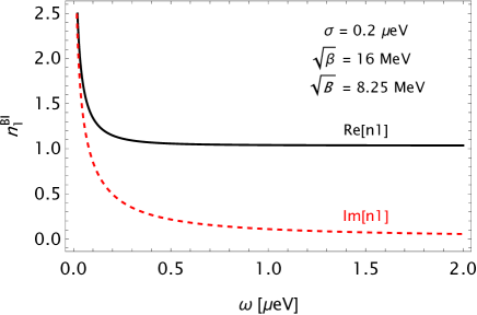
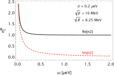
Figure 1: Left panel : The real (black line) and imaginary (red dashed line) parts of the solution $n_{1}$ as functions of the $\omega$-frequency. Right panel : The real (black line) and imaginary (red dashed line) parts of the solution $n_{2}$ as functions of the $\omega$-frequency. In both plots, we use $\sqrt{\beta}=16$ MeV, $\sqrt{|{\bf B}|}=8.25$ MeV, and $\sigma=0.2\,\mu\mbox{eV}$ for silver.

The solution of (16) is

$$n_{2}=\sqrt{\dfrac{1+\mathbf{B}^{2}/\beta^{2}-\sigma^{2}/\omega^{2}+i\,(2+\mathbf{B}^{2}/\beta^{2})\,(\sigma/\omega)}{1+(\mathbf{B}\cdot\mathbf{\hat{k}}/\beta)^{2}+i\,(\sigma/\omega)}}\;,$$ (20)

that has the real and imaginary parts

$$\Re[n_{2}] = \sqrt{\frac{|a|}{2}}\,\sqrt{\sqrt{1+\frac{b^{2}}{a^{2}}}+\mbox{sign}(a)}\;,$$ (21a)

$$\Im[n_{2}] = \sqrt{\frac{|a|}{2}}\,\sqrt{\sqrt{1+\frac{b^{2}}{a^{2}}}-\mbox{sign}(a)}\;,$$ (21b)

where $a$ e $b$ are read below

$$a\! = \!\dfrac{(1+\mathbf{B}^{2}/\beta^{2}-\sigma^{2}/\omega^{2})(\mathbf{B}\cdot\mathbf{\hat{k}})^{2}/\beta^{2}}{1+\sigma^{2}/\omega^{2}+[\,2+(\mathbf{B}\cdot\mathbf{\hat{k}})^{2}/\beta^{2}\,](\mathbf{B}\cdot\mathbf{\hat{k}})^{2}/\beta^{2}}$$ (22a)

$$+\;\,\dfrac{(1+\mathbf{B}^{2}/\beta^{2})\,(1+\sigma^{2}/\omega^{2})}{1+\sigma^{2}/\omega^{2}+[\,2+(\mathbf{B}\cdot\mathbf{\hat{k}})^{2}/\beta^{2}\,](\mathbf{B}\cdot\mathbf{\hat{k}})^{2}/\beta^{2}}\;,\hskip 19.91684pt$$

$$b\! = \!\frac{\sigma}{\omega}\,\dfrac{1+\sigma^{2}/\omega^{2}+(\mathbf{B}\cdot\mathbf{\hat{k}})^{2}/\beta^{2}(2+\mathbf{B}^{2}/\beta^{2})}{1+\sigma^{2}/\omega^{2}+[2+(\mathbf{B}\cdot\mathbf{\hat{k}})^{2}/\beta^{2}](\mathbf{B}\cdot\mathbf{\hat{k}})^{2}/\beta^{2}}\;,\hskip 25.6073pt$$ (22b)

and $\mbox{sign}(a)=a/|a|$ is the sign function of $a$. The real parts (19a) and (21a) contains the solutions of the dispersion relation, the wavelength and the group velocity of the wave. The imaginary parts (19b) and (21b) define the wave penetration in a conductor medium as $d=(\Im[n_{i}])^{-1}\,(i=1,2)$. The limit $\beta\rightarrow\infty$ in (19a)-(19b), and in (21a)-(21b), recovers the known results of the Maxwell ED:

$$\lim_{\beta\rightarrow\infty}\Re[n_{1}]=\Re[n_{2}]=\sqrt{\sqrt{\frac{1}{4}+\frac{\sigma^{2}}{4\omega^{2}}}+\frac{1}{2}}\;,$$ (23a)

$$\lim_{\beta\rightarrow\infty}\Im[n_{1}]=\Im[n_{2}]=\sqrt{\sqrt{\frac{1}{4}+\frac{\sigma^{2}}{4\omega^{2}}}-\frac{1}{2}}\;.$$ (23b)

The results (19a)-(19b) and (21a)-(21b) show the dependence of the real and imaginary parts with the angle $(\theta)$ that the magnetic background does with the wave propagation direction, i.e., $\cos\theta=\hat{{\bf k}}\cdot\hat{{\bf B}}$. In the case of ${\bf k}$ parallel to ${\bf B}$, the contribution of the $\beta$-BI parameter disappears in (19a) and $(\ref{Imn1})$. Under this particular condition, the solutions (21a) and (21b) keep the non-linear contribution. Under an intense magnetic field, the condition $|{\bf B}|\gg\beta$ reduces the results to expressions

$$\Re[n_{1}]=\Re[n_{2}]=\frac{1}{|\cos\theta|}\,\sqrt{\sqrt{\frac{1}{4}+\frac{\sigma^{2}}{4\omega^{2}}}+\frac{1}{2}}\;,$$ (24a)

$$\Im[n_{1}]=\Im[n_{2}]=\frac{1}{|\cos\theta|}\,\sqrt{\sqrt{\frac{1}{4}+\frac{\sigma^{2}}{4\omega^{2}}}-\frac{1}{2}}\;.$$ (24b)

These particular cases show that when the magnetic field is intense, the results of the Maxwell ED in a conductor are modified by the $\theta$-angle, and it does not depend on the magnetic field magnitude.

Thereby, we illustrate the real and imaginary parts of $n_{1}$ (left panel) and $n_{2}$ (right panel) as functions of the $\omega$-frequency in the fig. (1). The fig. (1) is set with the values of $\sqrt{\beta}=16\,\mbox{MeV}$ for propagation effects in BI ED, $\sqrt{B}=8.25\,\mbox{MeV}$ for a magnetic field of a neutron star, and $\sigma=0.2\,\mu\mbox{eV}$ for silver in natural units . The left panel in (1) shows that, when the magnetic field is perpendicular to the wave propagation direction, the $\Im[n_{1}]$ part decays for high frequencies in relation to $\Re[n_{1}]$, i. e., the dispersion and absorption of the wave go to zero in the high-energy limit. The right panel in (1) illustrates the real and imaginary parts of the $n_{2}$-solution as functions of the $\omega$-frequency. In this case, we choose the magnetic field parallel to the direction of the wave propagation direction.

IV The wave dispersion in the presence of an magnetic current

In this section, we study the dispersion effects for the case of a magnetic conductivity current. The nature of this current density is associated with the chirality between left- and right-handed fermions when it is submitted to an external magnetic field [19]. The magnetic current density is given by

$$\mathbf{J}=\sigma_{b}\,\mathbf{B}_{0}\;,$$ (25)

where $\sigma_{b}$ is the magnetic conductivity, that we consider isotropic throughout the material. Using the prescription of the magnetic background, with $\mathbf{B}_{0}=\mathbf{b}+\mathbf{B}$, the linearized equations in the presence of the current density (25) are read below

$$\mathbf{k}\cdot{\mathbf{e_{0}}}+\frac{1}{\beta^{2}}\;(\mathbf{B}\cdot\mathbf{k})(\mathbf{B}\cdot\mathbf{e_{0}})\! = \rho_{0}(k)\,,$$ (26a)

$$\mathbf{k}\times{\mathbf{e_{0}}} = \omega\,\mathbf{b_{0}}\;,$$ (26b)

$$\mathbf{k}\cdot{\mathbf{b_{0}}} = 0\,\hskip 5.69046pt,\hskip 5.69046pt$$ (26c)

$$\mathbf{k}\times{\mathbf{b_{0}}}+\frac{(\mathbf{B}\times\mathbf{k})(\mathbf{B}\cdot{\mathbf{b_{0}}})}{\beta^{2}+{\bf B}^{2}}\!\!\! = \!\!\!-i\,\sigma_{b}\,\mathbf{b_{0}}$$

$$-i\,\sigma_{b}\,\mathbf{B}\,\delta^{3}(\mathbf{k})\,\delta(\omega)-\frac{\omega}{\beta^{2}}\,\mathbf{B}\,(\mathbf{B}\cdot\mathbf{e_{0}})-\omega\,\mathbf{e_{0}}\;,$$ (26d)

where we have substituted the plane wave solutions via Fourier transform for the propagating EM fields $\mathbf{e}$, $\mathbf{b}$ and the charge density $\rho$. Combining these equations, we obtain the wave equation for the electric amplitude $e_{0j}$ :

$$O_{i\,j}\,e_{0j}=0\;,$$ (27)

where the matrix elements $O_{ij}$ are read below

$$O_{i\,j}\!\! = \!\!\left(1-\mathbf{n}^{2}\right)\,\delta_{ij}+n_{i}\,n_{j}-i\,\frac{\sigma_{b}}{\omega}\,\epsilon_{ijk}\,n_{k}$$ (28)

$$+\dfrac{(\mathbf{B}\times\mathbf{n})_{i}\,(\mathbf{B}\times\mathbf{n})_{j}}{\mathbf{B}^{2}+\beta^{2}}+\frac{1}{\beta^{2}}\,\mathbf{B}_{i}\,\mathbf{B}_{j}\;.$$

The non-trivial solution of (27) requires the condition $\det(O_{ij})=0$. The correspondent solutions are given by

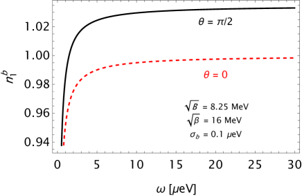
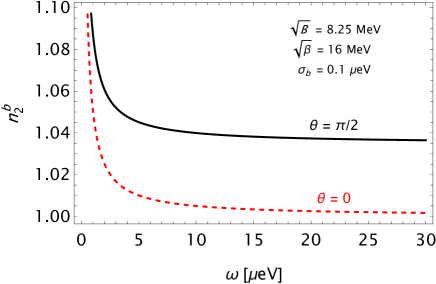
Figure 2: Left panel : The $n_{1}$-solution from (29a) as function of the $\omega$-frequency. Right panel : The $n_{2}$-solution from (29b) as function of the $\omega$-frequency. In both plots, the solid black line means the case of ${\bf B}\cdot{\bf k}=0$ (perpendiculars), whereas the dashed red lines set the case of ${\bf B}\times{\bf k}=0$ (parallels). We choose the parameters as $\sqrt{\beta}=16$ MeV, $\sqrt{|{\bf B}|}=8.25$ MeV, and $\sigma_{b}=0.1\,\mu\mbox{eV}$.

$$n_{1}\!\! = \!\!\sqrt{\frac{(\beta^{2}+\mathbf{B}^{2})\,\left(1+\,\frac{\sigma_{b}^{2}}{2\omega^{2}}-\frac{\sigma_{b}}{2\omega}\sqrt{4+\frac{\sigma_{b}^{2}}{\omega^{2}}}\right)}{\beta^{2}+(\mathbf{B}\cdot\mathbf{\hat{k}})^{2}}}\;,\hskip 28.45274pt$$ (29a)

$$n_{2}\!\! = \!\!\sqrt{\frac{(\beta^{2}+\mathbf{B}^{2})\,\left(1+\,\frac{\sigma_{b}^{2}}{2\omega^{2}}+\frac{\sigma_{b}}{2\omega}\sqrt{4+\frac{\sigma_{b}^{2}}{\omega^{2}}}\right)}{\beta^{2}+(\mathbf{B}\cdot\mathbf{\hat{k}})^{2}}}\;.\hskip 28.45274pt$$ (29b)

Notice that, both solutions are reals refractive index, and there is no absorption in this case of an isotropic magnetic conductivity. In $n_{1}$ and $n_{2}$, also emerge the dependence on the $\theta$-angle that $\mathbf{B}$ does with $\mathbf{\hat{k}}$-direction. In the case of $\mathbf{B}$ parallel to $\mathbf{\hat{k}}$, the non-linear contribution of the $\beta$-parameter is canceled in (29a) and $(\ref{n2 b})$. For $\mathbf{B}$ perpendicular to $\mathbf{\hat{k}}$, the $\beta$-parameter and the magnetic background contribute to the solutions. The solution $n_{1}$, when $\mathbf{B}\cdot\mathbf{k}=0$ (black line), and when $\mathbf{B}\times\mathbf{k}={\bf 0}$ (red line) are both showed in the fig. (2). In this plot, we choose $\sqrt{\beta}=16\,\mbox{MeV}$, $\sqrt{|{\bf B}|}=8.25\,\mbox{MeV}$, and $\sigma_{b}=0.1\,\mu\mbox{eV}$. In high frequency range, the curves goes to a maximum refractive index, that satisfies the condition $n_{1\perp}>n_{1\parallel}$, where $n_{1\perp}\simeq 1.034$, and $n_{1\parallel}\simeq 1.0$, when $\omega\rightarrow\infty$.

The $n_{2}$-solution is shown in the right panel from the fig. (2). The black line corresponds to $\mathbf{B}$ perpendicular to $\mathbf{\hat{k}}$, and the dashed red line is the case of $\mathbf{B}$ parallel to $\mathbf{\hat{k}}$. In this figure, we also consider $\sqrt{\beta}=16\,\mbox{MeV}$, $\sqrt{|{\bf B}|}=8.25\,\mbox{MeV}$ and $\sigma_{b}=0.1\,\mu\mbox{eV}$. In the right panel, the curves have a horizontal asymptotes for high energies, where $n_{2\perp}\simeq 1.034$ and $n_{2\parallel}\simeq 1.0$, for a high frequency range.

V Birefringence phenomenon

Since the refractive index depend on the $\theta$-angle that we have defined as $\cos\theta=\mathbf{B}\cdot\mathbf{\hat{k}}$, the birefringence phenomenon emerges from the solutions in both electric and magnetic conductivity current cases. In the case of the Ohmic current, we consider the real part of the solutions for the analysis of the birefringence. We define it as the difference between the parallel and perpendicular real part of the refractive indices

$$\delta n_{i}^{e}=\Re[n_{i\perp}^{e}]-\Re[n_{i\parallel}^{e}]\;,$$ (30)

where $i=\{\,1\,,\,2\,\}$, $n_{i\perp}^{e}$ is the refractive index when $\mathbf{B}$ is perpendicular to $\mathbf{\hat{k}}$, and $n_{i\parallel}^{e}$ denotes the refractive index when $\mathbf{B}$ is parallel to $\mathbf{\hat{k}}$. Substituting the real parts of (19a) and (21a), we obtain

$$\delta n_{1}^{e}\! = \!\left(\!\sqrt{1+\frac{{\bf B}^{2}}{\beta^{2}}}-1\!\right)\!\sqrt{\sqrt{\frac{1}{4}+\frac{\sigma^{2}}{4\omega^{2}}}+\frac{1}{2}}\;,$$ (31a)

$$\delta n_{2}^{e}\! = \!\sqrt{\sqrt{\frac{1}{4}+\frac{{\bf B}^{2}}{4\beta^{2}}+\frac{\sigma^{2}}{4\omega^{2}}}+\frac{1}{2}+\frac{{\bf B}^{2}}{2\beta^{2}}}$$ (31b)

$$-\sqrt{\sqrt{\frac{1}{4}+\frac{\sigma^{2}}{4\omega^{2}}}+\frac{1}{2}}\;.$$

It is worth to highlight that the birefringence disappears $\delta n_{i}^{e}=0$, when $\beta\rightarrow\infty$.

In the polarization vacuum with laser (PVLAS) experiment [21], the magnetic field is $|{\bf B}|=2.5\,\mbox{T}=1.7\times 10^{-9}\,\mbox{MeV}^{2}$ in which $\beta\gg|{\bf B}|$ in this case. Thereby, we can apply the results (31a) and (31b) in this approximation to obtain the result

$$\frac{\delta n_{1}^{e}}{B^{2}} \simeq \frac{1}{2\beta^{2}}\,\sqrt{\sqrt{\frac{1}{4}+\frac{\sigma^{2}}{4\omega^{2}}}+\frac{1}{2}}\;,$$ (32a)

$$\frac{\delta n_{2}^{e}}{B^{2}} \simeq \frac{1}{4\beta^{2}}\frac{\frac{2\sigma^{2}}{\omega^{2}}+2+\sqrt{1+\frac{\sigma^{2}}{\omega^{2}}}}{(1+\frac{\sigma^{2}}{\omega^{2}})\sqrt{2+2\sqrt{1+\frac{\sigma^{2}}{\omega^{2}}}}}\;.$$ (32b)

Using that $\delta n_{i}^{e}/B^{2}=(19\pm 27)\times 10^{-24}\,\mbox{T}^{-2}$ from the PVLAS experiment [21], the expression (32a) yields the acceptable numeric result for the electric conductivity over the frequency :

$$\frac{\sigma}{\omega}\simeq 56.75\;.$$ (33)

Similarly to (30), we define the birefringence in the case of magnetic conductivity as

$$\delta n_{i}^{b}=n_{i\perp}^{b}-n_{i\parallel}^{b}\;.$$ (34)

Using the solutions (29a) and (29b), the birefringence of $\delta n_{i}$ is given by solutions

$$\delta n_{1}^{b}\!\! = \!\!\left(\sqrt{1+\frac{{\bf B}^{2}}{\beta^{2}}}-1\right)\sqrt{1+\,\frac{\sigma_{b}^{2}}{2\omega^{2}}-\frac{\sigma_{b}}{2\omega}\,\sqrt{4+\frac{\sigma_{b}^{2}}{\omega^{2}}}}\;,$$

$$\delta n_{2}^{b}\!\! = \!\!\left(\sqrt{1+\frac{{\bf B}^{2}}{\beta^{2}}}-1\right)\sqrt{1+\,\frac{\sigma_{b}^{2}}{2\omega^{2}}+\frac{\sigma_{b}}{2\omega}\,\sqrt{4+\frac{\sigma_{b}^{2}}{\omega^{2}}}}\;.\;\;\;$$

Notice that, the birefringence disappears in the limit $\beta\rightarrow\infty$, or when the magnetic background is turned off. The birefringence curves as functions of the $\omega$-frequency are shown in figure (3). In this plot, we choose $\sqrt{\beta}=16\,\mbox{MeV}$, $\sqrt{|\mathbf{B}|}=8.25\,\mbox{MeV}$ and $\sigma_{b}=0.5\,\mu\mbox{eV}$.

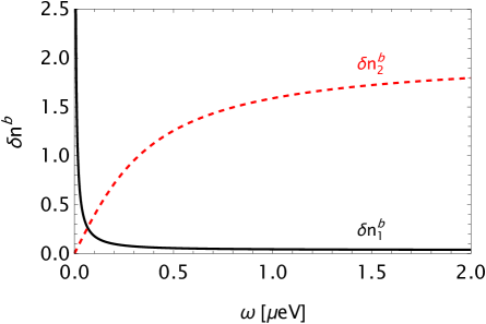
Figure 3: The birefringence curves for $\delta n_{1}^{b}$ (black line) and $\delta n_{2}^{b}$ (dashed red line) as functions of the $\omega$-frequency. We choose the values $\sqrt{\beta}=16\,\mbox{MeV}$, $\sqrt{|\mathbf{B}|}=8.25\,\mbox{MeV}$ and $\sigma_{b}=0.5\,\mu\mbox{eV}$.

The $\delta n_{1}$-solution has a minimum of birefringence at $\delta n_{1min}\simeq 0.034$, whereas $\delta n_{2}$ has a maximum birefringence at $\delta n_{2max}\simeq 2.034$, for high frequency $\omega\rightarrow\infty$.

Applying these results for the PVLAS experiment, the expressions (36a) and (36b) are simplified as

$$\frac{\delta n_{1}^{b}}{B^{2}}\!\! \simeq \!\!\frac{1}{2\beta^{2}}\,\sqrt{1+\,\frac{\sigma_{b}^{2}}{2\omega^{2}}-\frac{\sigma_{b}}{2\omega}\,\sqrt{4+\frac{\sigma_{b}^{2}}{\omega^{2}}}}\;,$$ (36a)

$$\frac{\delta n_{2}^{b}}{B^{2}}\!\! \simeq \!\!\frac{1}{2\beta^{2}}\,\sqrt{1+\,\frac{\sigma_{b}^{2}}{2\omega^{2}}+\frac{\sigma_{b}}{2\omega}\,\sqrt{4+\frac{\sigma_{b}^{2}}{\omega^{2}}}}\;,\;\;$$ (36b)

in which we have used the condition $\beta\gg|{\bf B}|$. Using that $\delta n_{i}^{b}/B^{2}=(19\pm 27)\times 10^{-24}\,\mbox{T}^{-2}$, for the case of the magnetic conductivity, we obtain the numeric result

$$\frac{\sigma_{b}}{\omega}\simeq 5.18\;.$$ (37)

VI Concluding comments

In this paper, we study the dispersion and absorption of waves in the linearized Born-Infeld (BI) electrodynamics governed by the Ohmic and magnet current densities. The linearization of the BI ED is introduced through the propagating electromagnetic field added to a uniform and constant magnetic background field. The BI non-linear lagrangian in expanded up to second order for small propagating effects, and around the magnetic background. Thus, we substitute the wave plane superpositions for the linearized electromagnetic field, and discuss the wave propagation properties in a material medium in the presence of the electric and magnetic conductivities.

From the wave equation, we calculate the refractive index solutions in terms of the magnetic background, of the BI parameter, and of the electric conductivity for the material medium. In this first case, the refractive index has a real and imaginary parts, that are interpreted as the dispersion and the absorption of the wave, respectively. In the second case, the magnetic current density for an isotropic magnetic conductivity is investigated in which there is no wave absorption. One fact is important : in all these solutions, the refractive index depends on the $\theta$-angle that the magnetic background ${\bf B}$ does with the wave propagation direction $\hat{{\bf k}}$, i. e., $\cos\theta=\hat{{\bf B}}\cdot\hat{{\bf k}}$. Thus, the solutions provide the situations in which ${\bf B}$ is parallel to ${\bf k}$, and ${\bf B}$ perpendicular to ${\bf k}$. It opens the discussion of the birefringence phenomenon, that depends on the BI parameter, and on the magnetic background. When the BI parameter is removed, the birefringence is null, and as well, all the results of the Maxwell ED are recovered.

In the birefringence analysis, we use the known result from the PVLAS experiment for the vacuum birefringence $\Delta n/B^{2}=(19\pm 27)\times 10^{-24}\,\mbox{T}^{-2}$ to estimate the ratio of electric and magnetic conductivities over the wave $\omega$-frequency. Under these conditions, we consider a weak magnetic field of $2.5\,\mbox{T}$ and the BI parameter of $\sqrt{\beta}=16$ MeV. The result for the birefringence associated with the electric conductivity yields the numeric result $\sigma/\omega=56.75$, whereas for the case of the magnetic conductivity, the birefringence yields the result $\sigma_{b}/\omega=5.18$ for a large range of frequency. For end, this paper opens the discussion of applications of these refractive index solutions in others non-linear electrodynamics, as Euler-Heisenberg and ModMax EDs. Other perspective is to investigate the effects of the linearization in optics classical law where the medium is affected by the external magnetic field. This is one of the discussions for a forthcoming project.

References

• [1] M. Born and L. Infeld, Proc. R. Soc. Lond. Ser. A 144, 425 (1934).
• [2] H. Euler and W. Heisenberg, Z. Phys. 98, 714 (1936).
• [3] D. P. Sorokin, Fortsch. Phys. 70 (2022) 2200092.
• [4] John Ellis, Nick E. Mavromatos and Tevong You, Phys. Rev. Lett. 118 (2017) 261802.
• [5] A. A. Tseytlin, Yuri Golfand Memorial Volume, Edited by M. Shifman, University of Minnesota, 2000.
• [6] E. S. Fradkin and A. A. Tseytlin, Phys. Lett. B 163, 12 (1985).
• [7] E. Bergshoeff, E. Sezgin, C. N. Pope and P. K. Townsend, Phys. Lett. B 188, 70 (1987).
• [8] A. C. Keser, Y. Lyanda-Geller and O. P. Sushkov, Phys. Rev. Lett. 128 (2022) 066402.
• [9] Z. Zhao, Q. Pan, S. Chen and J. Jing, Nucl. Phys. B 871, 98 (2013).
• [10] Z. Bialynicka-Birula and I. Bialynicki-Birula, Phys. Rev. D 2 (1970) 2341.
• [11] Xue-Peng Hu and Yi Liao, Eur. Phys. J. C 53 635-639 (2008).
• [12] M. J. Neves, Jorge B. de Oliveira, L. P. R. Ospedal and J. A. Helayël-Neto, Phys. Rev. D 104 (2021) 015006.
• [13] J. M. A. Paixão, L. P. R. Ospedal, M. J. Neves and J. A. Helayël-Neto, JHEP 2022 160 (2022).
• [14] M. J. Neves, P. Gaete, L. P. R. Ospedal and J. A. Helayël-Neto, Phys. Rev. D 107 (2023) 075019.
• [15] A. Zangwill, Modern Electrodynamics. New York (USA): Cambridge University Press, 2012.
• [16] D. E. Kharzeev, Prog. Part. Nucl. Phys. 75, 133 (2014).
• [17] D. E. Kharzeev, J. Liao, S. A. Voloshin, and G. Wang, Prog. Part. Nucl. Phys. 88 1 (2016).
• [18] D. Kharzeev, K. Landsteiner, A. Schmitt and H.U. Yee, Lect. Notes Phys. 871 (Springer-Verlag,Berlin Heidelberg,2013).
• [19] A. A. Burkov, J. Phys. Condens. Matter 27, 113201 (2015).
• [20] Pedro D. S. Silva, Manoel M. Ferreira Jr. and Marco Schreck, Phys. Rev. D 102, 076001 (2020).
• [21] A. Ejlli, F. Della Valle, U. Gastaldi, G. Messineo, R. Pengo, G. Ruoso and G. Zavattini, Phys. Rep. 871 (2020) 1.